Optimizing Streaming Parallelism on Heterogeneous Many-Core Architectures: A Machine Learning Based Approach

Peng Zhang, Jianbin Fang, Canqun Yang, Chun Huang, Tao Tang, Zheng Wang Peng Zhang, Jianbin Fang, Canqun Yang, Chun Huang, and Tao Tang are with National University of Defense Technology, China.
E-mail: {zhangpeng13a, j.fang, canqun, chunhuang}@nudt.edu.cn Zheng Wang is with University of Leeds, United Kingdom.
E-mail: z.wang5@leeds.ac.uk

Abstract

As many-core accelerators keep integrating more processing units, it becomes increasingly more difficult for a parallel application to make effective use of all available resources. An effective way for improving hardware utilization is to exploit spatial and temporal sharing of the heterogeneous processing units by multiplexing computation and communication tasks – a strategy known as heterogeneous streaming. Achieving effective heterogeneous streaming requires carefully partitioning hardware among tasks, and matching the granularity of task parallelism to the resource partition. However, finding the right resource partitioning and task granularity is extremely challenging, because there is a large number of possible solutions and the optimal solution varies across programs and datasets. This article presents an automatic approach to quickly derive a good solution for hardware resource partition and task granularity for task-based parallel applications on heterogeneous many-core architectures. Our approach employs a performance model to estimate the resulting performance of the target application under a given resource partition and task granularity configuration. The model is used as a utility to quickly search for a good configuration at runtime. Instead of hand-crafting an analytical model that requires expert insights into low-level hardware details, we employ machine learning techniques to automatically learn it. We achieve this by first learning a predictive model offline using training programs. The learnt model can then be used to predict the performance of any unseen program at runtime. We apply our approach to 39 representative parallel applications and evaluate it on two representative heterogeneous many-core platforms: a CPU-XeonPhi platform and a CPU-GPU platform. Compared to the single-stream version, our approach achieves, on average, a 1.6x and 1.1x speedup on the XeonPhi and the GPU platform, respectively. These results translate to over 93% of the performance delivered by a theoretically perfect predictor.

Index Terms:

Heterogeneous computing; Parallelism; Performance Tuning; Machine learning

1 Introduction

Heterogeneous many-cores, as representative by GPGPUs and Intel’s XeonPhi, are widely used for accelerating parallel applications [1, 2, 3]. As users demand higher performance, many-core accelerators have become more powerful by providing more and more processing units. While the abundant computing resources offer the potential for higher performance, it becomes harder for a parallel application to utilize all the available computing resources [4, 5]. As a result, many parallel applications fail to fully unlock the performance potential of a many-core accelerator.

One way for improving heterogeneous many-core utilization is to exploit spatial and temporal sharing of processing resources. This strategy is also known as heterogeneous streaming [6]. The idea is to exploit the computation and communication independency of task parallelism to improve hardware utilization. It works by partitioning the processor cores to allow independent communication and computation tasks (i.e. streams) to run concurrently on different hardware resources, which effectively overlaps the concurrent kernel execution with data movements. Representative heterogeneous streaming implementations include CUDA Streams [7], OpenCL Command Queues [8], and Intel heterogeneous streams library (hStreams) [9, 6]. These implementations allow a parallel program to spawn more than one stream (or pipeline) so that the data movement stage of one pipeline overlaps the kernel execution stage of another.

Prior work on heterogeneous streaming mainly targets GPUs [10, 11, 12]. Compared to GPU implementations, OS-enabled coprocessors, like the Intel XeonPhi, provides some unique features that are currently unavailable on the GPU. For example, besides specifying the number of streams, developers can explicitly map streams to different groups of cores on XeonPhi to control the number of cores of each hardware partition. This parameter is not exposed to programmers on GPUs, making previous work on GPU-based parallel streaming optimizations infeasible to fully exploit Xeon-Phi-like many-core accelerators (see also Section 6.3). On the other hand, ample evidence is showing that choosing the right stream configuration, i.e., the number of processor core partitions and the number of concurrent tasks of a multi-stream application, values, has a significant impact the application’s performance on many-core architectures [13, 14, 15]. However, attempting to find the optimal values through exhaustive profiling would be ineffective, because the range of the possible values for the two parameters is huge. What we need is a technique that automatically determines the optimal stream configuration for any streamed application in a fast manner.

This article presents a novel approach to determine the right number of processor core partitions and tasks for heterogeneous streams, targeting heterogeneous many-core architectures. Our key insight is to use a performance model to quickly search for the optimal stream configuration. The performance model estimates the resulting performance of the target streamed application when it runs under a given stream configuration. If the prediction can be performed quickly with low overhead, we can then quickly explore a large configuration space. Instead of hand-crafting the performance model that requires human modification whenever the architecture evolves (i.e., when the number and types of cores change), we employ machine learning techniques to automatically construct a predictive model. Our predictor is first trained off-line. Then, using code and dynamic runtime features of the program, the model predicts performance for a new, unseen program under a given stream configuration.

Our prior work [16] develops a machine learning based classifier to predict the optimal stream configuration. However, this approach can only choose from a limited set of configurations seen during the training phase. Unlike a classification-based approach, the approach presented in the article allows us to explore a larger number of stream configurations (including those that are not seen during the training phase) with negligible runtime overhead. This advantage significantly improves the generalization ability of the proposed approach (Section 3).

Due to the newness of heterogeneous streaming execution model, there are very few multi-stream benchmarks available. To evaluate our approach on a wide range of applications, we have developed a compiler-based tool to automatically translate standard OpenMP benchmarks into their streamed variants for the backends of XeonPhi and GPU architectures (Section 4). With the help of this code generator, we can apply our approach to 39 parallel benchmarks. We argue that this tool can help generate more streamed code and thus is an added value to the community.

We evaluate our approach on two representative heterogeneous many-core platforms: a 57-core Intel XeonPhi and an NVIDIA 1080Ti GPU platforms. We achieve, on average, a 1.6x and 1.1x speedup over the single-stream execution on the XeonPhi and the GPU platforms, respectively. This translates to over 93% of the best available performance.

The core contribution of this paper is a novel machine-learning-guided approach for automatically determining the optimal stream configuration on heterogeneous many-cores. We show that our approach delivers good performance across benchmarks and heterogeneous many-core platforms. While we do not seek to advance the machine learning algorithm itself, our work shows how machine learning can be used to address the challenging problem of tuning fine-grained streaming parallelism on heterogeneous many-core architectures. In this work, we demonstrate the usefulness of our approach on XeonPhi and an NVIDIA GPU, but our approach is equally applicable on other heterogeneous platforms like AMD GPUs.

2 Background and Overview

In this section, we first give a brief introduction of heterogeneous streaming; we then define the scope of this work, before motivating the need of our scheme and providing an overview of our approach.

2.1 Heterogeneous Streaming

The idea of heterogeneous streaming is to exploit spatial and temporal sharing of computing resources to utilize the hardware resources to improve application performance.

Spatial Sharing. Modern many-core accelerators offer a large number of processing units. Since many applications cannot fully utilize all the cores at a time, we can partition the computing units into multiple groups to concurrently execute multiple tasks. In this way, the computing resource is spatially shared across concurrently-running application tasks. The key to spatial sharing is to determine the right number of partitions, because over-provisioning of processing units would waste computing resources but under-provisioning would lead to slowed down performance.

Temporal Sharing. Code written for heterogeneous computing devices typically consists of several stages, such as host device communication and computation. Using temporal sharing, one can overlap some of these stages to exploit pipeline parallelism to improve performance by overlapping the host-device communication and kernel execution.

⬇ 1//setting the partition-size and task granularity hStreams_app_init(partition_size,streams_p_part); 3 //stream queue id 5stream_id = 0; for(…){ 7 //enquque host-device transfer to current stream hStreams_app_xfer_memory(,,, stream_id, HSTR_SRC_TO_SINK,…); 9 … //enqueue computation to the current stream 11 hStreams_EnqueueCompute(stream_id, ”kernel1”, …); … 13 //move to the next stream stream_id = (stream_id++) % MAX_STR; 15} //transfer data back to host 17hStreams_app_xfer_memory(,,, HSTR_SINK_TO_SRC,…);

Figure 1: Heterogeneous streaming using hStreams as an example.

2.2 Problem Scope

Our work aims to improve the performance of a data parallel application by exploiting spatial and temporal sharing of heterogeneous streams. We do so by determining at runtime how many partitions should be used to group the cores (#partitions) and how many data parallel tasks (#tasks) should be used to run the application. Our current implementation is applicable to XeonPhi and GPUs by using different runtime back-ends (hStream for XeonPhi, and CUDA or OpenCL for GPUs).

Code Example. Figure 1 gives a simplified code example written with Intel’s hStreams APIs that can run on the XeonPhi many-core. At line 2 we initialize the stream execution by setting the number of partitions and tasks/streams per partition. This initialization process essentially creates multiple processor domains and determines how many logical streams can run on a partition. In the for loop (lines 7-14) we enqueue the communication and computation tasks to a number of streams identified by the stream_id variable. In this way, communication and computation of different streams can be overlapped during execution (temporal sharing); and streams on different processor domains (or partitions) can run concurrently (spatial sharing). Our predictive model determines the #partitions and the #tasks before invoking the hStreams initialization routine, hStreams_app_init().

2.3 Motivating Examples

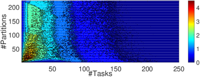
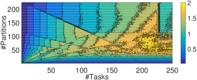
Consider Figure 2 which shows the resultant performance improvement given by multi-stream parallelism over the single-stream version of the code for two applications on a 57-core Intel XeonPhi system. We use two streamed programs from prior work [13]: binomial computes the price evolution over a given period and prefixSum calculates the prefix sum for a sequence of numbers.

It is observed from this example that not all multi-stream configurations give improved performance. As can be seen from the diagrams, the search space of multi-stream configurations is huge but good configurations are sparse. The performance varies significantly over stream configurations (#partitions, #tasks). The optimal #tasks for binomial ranges from 1 to 30, and the best #partitions is between 1 and 40. In contrast to binomial, prefixsum benefits from fine-grained parallelism when using a larger #tasks (220 to 224) and #partitions (60 to 80). However, the stream configurations that are effective for prefixsum give no speedup over the single-stream version for binomial.

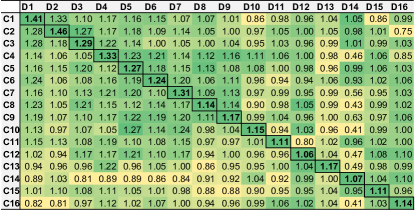
Now consider Figure 3 that shows the speedups of dct under 16 multi-stream configurations over the single-stream version, where each configuration is found to give the best-performance for one of the 16 inputs. In the color table, each cell shows the performance of a stream configuration ( $C1,...,C16$ ) on a specific input dataset ( $D1,...,D16$ ); and the values along the diagonal line represent the best-available performance (found through profiling) for an input. As can be seen from the figure, the best stream configuration can vary across inputs for the same benchmark. For example, while $C4$ gives a speedup of 1.33x over the baseline for dataset $D4$ , it delivers a poor performance for dataset $D14$ by doubling the execution time over the single-stream version. This diagram also suggests that no single configuration can give improved performance for all inputs.

Lesson Learned. These two examples show that choosing the stream configuration has a great impact on performance and the best configuration must be determined on a per-program and per-dataset basis. Later, we will show that this observation is not unique to XeonPhi but also holds for GPUs. Attempting to find the optimal configuration through means of an exhaustive search would be ineffective, and the overhead involved would be far bigger than the potential benefits. Online search algorithms, while can speed up the search process, the overhead can still outweigh the benefit. For example, when applying simulated annealing to binomial, the best-found configuration only reaches 84% of the best-available performance after 310,728 iterations¹¹1In Section 6.1, we show that our approach achieves 93% of the best-available performance for binomial on XeonPhi.. Classical hand-written heuristics are not ideal either, as they are not only complex to develop, but are likely to fail due to the variety of programs and the ever-changing hardware architecture. An alternate approach, and the one we chose to use, is to use machine learning to automatically construct a performance model to estimate the benefit of any candidate configuration, providing minimal runtime overhead for searching for a good configuration, and having little development cost when targeting new architectures.

2.4 Overview of Our Approach

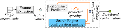
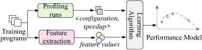
Our library-based approach, depicted in Figure 4, is completely automated. To determine the best streaming configuration, our approach follows a number of steps described as follows. We use a set of information or features to capture the characteristics of the program. We develop a LLVM [17] compiler pass to extract static code features at compile time, and a low-overhead profiling pass to collect runtime information at execution time (i.e., during the first few loop iterations). Because profiling also contributes to the final program output, no computation cycle is wasted. At runtime, we search for a good configuration through an offline trained performance model to estimate the resulting performances for all candidate configurations. The performance model takes in the feature values, a given configuration of resource partition and task granularity and estimates the potential speedup for the given configuration over the single-stream version. The overhead of runtime feature collection and search is a few milliseconds, which is included in all our experimental results. Since our training process can be performed automatically, we can easily target our performance model for different architectures.

3 Performance Modeling

At the core of our approach is a machine learned performance model built upon the Multi-layer Perceptron (MLP) artificial neural network (ANN). Our prototype is implemented using the Python scikit-learn machine learning package [18]. It is to note that our prior work [16] uses a Support Vector Machine (SVM) based classifier. However, such an approach can only make predictions on a limited set of configurations seen at the training time. Unlike a classification-based approach, the new approach presented in this article is a regression-based model which can make predictions on any stream configuration. This new approach thus has a better generalization ability for various heterogeneous architectures. We have also evaluated a number of alternative modeling techniques, including MLP, SVM, and decision trees. We chose MLP because it gives the best performance and has modest training overhead (see Section 6.6.1).

Our performance model takes as input the feature values and a given configuration (e.g., #partitions and #tasks for XeonPhi and #tasks for GPUs). It predicts the speedup for the given configuration. Building and using such a model follows a 3-step process for supervised learning: (i) generate training data (ii) train a performance model (iii) use the performance model, described as follows.

3.1 Training the Performance Model

Our method for model training is shown in Figure 5. To learn a regression model, we first need to profile the execution time (in order to calculate the speedup over the single-stream version) of all candidate configurations for each training program, and extract the feature values from the program. We then use the feature values, configuration settings and speedups to train a model.

3.1.1 Generating Training Data

To generate training data, we apply cross-validation to 39 benchmarks, i.e., by excluding the testing benchmarks from the training dataset (see also Section 5.3.1). We execute each training program and benchmark a number of times until the gap of the upper and lower confidence bounds is smaller than 5% under a 95% confidence interval setting. We then calculate the average speedup for a given stream configuration over the single-stream version. We exhaustively execute each training program across a wide range of stream configurations, and record the performance of each. Next, we calculate the speedup for each configuration, program and dataset. Finally, we extract the values of our selected set of features from each program and dataset. We stress that the trained model can be applied to stream configurations that are not seen in the training phase.

3.1.2 Profiling Configurations

During the training phase, we exhaustively execute each training program across a set of streamed configurations. On XeonPhi, we profile each training program using the #partitions ranging from 1 to 224 (the maximum number of physical threads on XeonPhi) and the #tasks ranging from 1 to 256 ²²2We chose these values because configuration settings beyond these values give a poor performance during our initial evaluation.. On GPUs, we cannot configure the number of partitions currently, we set the #partitions to the same as #tasks to be consistent with XenPhi. On this platform, we also set the #tasks to be range between $2^{0}$ and $2^{10}$ , which is big enough to include the optimal values according to our experiments. Note that these parameter ranges can be configured by the user.

3.1.3 Building The Model

Each evaluated configuration is appended to the feature value vector of a training program to form a model input. The model inputs and the corresponding speedups (i.e., ground truths) for all training programs are passed to a learning algorithm. The algorithm finds a correlation between the input vector and the desired prediction. The output of our learning algorithm is an MLP model where the weights of the model are determined from the training data. Model parameter tuning is performed on the training dataset for each targeting hardware architecture, using cross-validation (see also Section 6.6.3). In our case, the overall training process for all the 39 training programs (which is dominated by training data generation) takes less than a week on a single machine. Since training is performed only once “at the factory”, this is a one-off cost.

3.2 Features

Our performance models are based exclusively on code and dynamic features of the target programs. Code features are extracted from the program source code, and dynamic features are collected using hardware performance counters during the initial profiling run of the target application. We restrict us in using hardware performance counters that are commonly available on modern processors such as the data cache misses to ensure that our approach can be applied to a wide range of many-core architectures.

We considered 38 candidate raw features in this work. Some features were chosen from our intuition based on factors that can affect the performance such as dts (host-device data transfer size) and #xfer_mem, while other features were chosen based on previous work [19, 20].

3.2.1 Feature Selection

To build an accurate model through supervised learning, the training sample size typically needs to be at least one order of magnitude greater than the number of features. In this work, we start from 311 training samples and 38 raw features, so we would like to reduce the number of features in use. Our process for feature selection is fully automatic, described as follows.

We first combine several raw features to form a set of combined normalized features, which are able to carry more information than the individual parts. For example, instead of reporting raw branch hit and miss counts, we use the branch miss rate. Next, we removed raw features that carried similar information which is already captured by chosen features. To find which features are closely correlated, we constructed a correlation coefficient matrix using the Pearson correlation coefficient [21]. The closer a coefficient between two features is to +/-1, the stronger the correlation between the two input features. We removed any feature which had a correlation coefficient (taking the absolute value) greater than 0.7. Similar features include the number of executed instructions and the number of E-stage cycles that were successfully completed.

Our feature selection process reduces the number of features to 10 for XeonPhi (see Table I) and 10 for the NVIDIA Titan 1080Ti GPU (see Table II), where some features are shared. Since our approach for feature selection is automatic, the approach can be applied to other sets of candidate features. It is to note that feature selection is also performed using cross-validation (see also Section 5.2).

Table I: Chosen features for XeonPhi performance model

Feature	Description
loop nest	at which level the outermost parallelizable loop lies on
loop count	# of the parallel loop iterations
#xfer_mem	# of host-device transfer API calls
dts	total host-device transfer size
redundant transfer size	host-device transfer size among overlapping tasks
max blocks	the maximum number of tasks of the application
min task unit	the minimum task granularity for a partition
# instructions	the total number of instructions of the kernel
branch miss	branch miss rate
L1 DCR	L1 Data cache miss rate

Table II: Chosen features for GPU programs

Feature	Description
Access type 1	# array access, whose fastest varying index is an affine function of the block id
Access type 2	#array accesses, whose second or higher dimensional index is an affine function of the block id
#xfer_mem	# of host-device transfer API calls
host to device transfer size	total host to device transfer size
device to host transfer size	total device to host transfer size
redundant transfer size	host-device transfer size among overlapping tasks
max blocks	the maximum number of tasks
# instructions	the total number of instructions of the kernel
divergent branches	# divergent branches
L2 read miss rate	L2 cache read miss rate

3.2.2 Feature Standardization

Supervised learning typically requires the feature values to lie in a certain range. Therefore, we scaled the value for each of our features between the range of 0 and 1. We record the maximum and minimum value of each feature found at the training phase, and use these values to scale features extracted from a new application after deployment. We truncate a value during deployment if the value is outside the minimum/maximum value range seen during training. It is to note that we also use the same approach to normalize the model predictions (speedups) to the range of 0 and 1. In this work, we choose Z-score to standardize the training data, and the details of quantifying the impact of feature engineering methods can be found in Section 6.6.2.

3.2.3 Feature Importance

To understand the usefulness³³3In Section 6.6.4, we give a further breakdown of the impact of individual feature to the model performance on a per benchmark basis. of each feature, we apply a factor analysis technique called Varimax rotation [22] to the feature space transformed by the principal component analysis (PCA). This technique quantifies the contribution of each feature to the overall variance in each of the PCA dimensions. Intuitively, the more variances a feature brings to the space, the more useful information the feature carries.

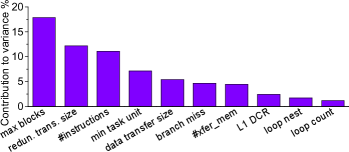
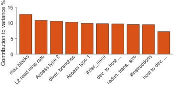
As an example, Figure 6 shows the top features chosen for XeonPhi and NVIDIA GPU architectures. For the XeonPhi platform, features that capture the parallelism degree (e.g. max blocks), host-device communication (e.g. redundant transfer size), and computation (e.g. #instructions) are found to be important. Other features such as L1 DCR and loop nest are useful, but are less important compared to others. On the NVIDIA GPU platform, we note that the parallelism degree is important, and the other features are equally useful (Figure 6b). This figure shows that prediction can accurately draw upon a subset of aggregated feature values.

3.3 Runtime Deployment

Once we have built and trained our performance model as described above, we can use it as a cost function to search for the best stream configuration for any new, unseen program. Feature values are extracted from the single-stream version of the code. Static code features (such as loop count) are extracted from the program source at compile time. Dynamic features (such as branch miss) are extracted by profiling the program without partitioning for a few loop iterations (which typically translate to several microseconds). After feature collection, we feed the feature values to the search engine to rank all candidate configurations using the performance model. The top-ranked stream configuration is then used for the target program. In Section 4.4, we provide further details on how the performance model can be integrated with the host code generation process.

3.3.1 Adapt to Changing Program Phases

Our current implementation chooses a configuration for each kernel and does not change the configuration throughout the kernel execution. Therefore, it can adapt to different behaviors across kernels because predictions are performed on a per-kernel basis. We found that this strategy is sufficient for many data-parallel kernels targeted in this work.

Our approach can be extended to adapt phase or program behavior changes within a kernel. One way of doing this is to first partition the input data into groups and then perform configuration selection before launching the kernel that performs on an input data group. To reduce the prediction and configuration overhead, we can sample periodically to see if the performance counter readings are significantly different from the ones used for the current prediction to trigger re-configuration. Dynamic re-configuration of a running kernel will require extending the underlying runtime (e.g., hStreams or CUDA) to adjust thread mapping and having hardware support to stop and resume the execution contexts. We leave this as future work.

4 OpenMP to Streamed Code Generator

Currently, there are very few publicly available benchmarks for utilizing the streaming capability of heterogeneous many-core architectures, in particular, XeonPhi. To evaluate our approach on a diverse set of benchmarks, we have developed a compiler-based code generator, autostreamer, to automatically translate OpenMP programs onto streamed code depending on the target architecture. Our code generator is open sourced⁴⁴4Available at: https://github.com/wisdom-moon/autostreamer.. Our implementation currently supports converting OpenMP code to hStreams, CUDA and OpenCL programs. While we do not claim novelty on this as several works on source-to-source translation from OpenMP to CUDA[23, 24, 25, 26] or OpenCL[20, 27] exist, we believe the tool could serve as a useful utility for translating OpenMP programs to exploit multi-stream performance on heterogeneous many-core architectures.

4.1 Code Generator Overview

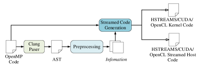
Figure 7 depicts our source to source code generator for translating OpenMP code to streamed programs. We use LLVM’s Clang front-end to convert OpenMP code into the abstract syntax tree (AST). We then traverse the AST to obtain the information to generate candidate streamed kernels and host-device management code. The generated kernel and host code make use of exiting programming models for kernel launching and communication management. We use hStreams for XeonPhi and CUDA or OpenCL for GPUs.

Our current implementation supports the translation of OpenMP parallel loops, i.e., loops annotated with omp for or omp for reduction constructs. For each parallel loop, we outline the loop body and translate it into an individual kernel function. We then replace the original loop body with a function call (running on the host CPU) to launch the generated kernel. We also generate management code for streaming context initialization, data partitioning, data movements between the host and the accelerator, etc.

Our code generator relies on the native host/device compiler to optimize the generated code. We have also compared our automatically generated code against the manually translated code used in our prior work [16] and found that there is little difference in performance for the set of OpenMP benchmarks used in this work.

4.2 Preprocessing

As an example, Figure 8 illustrates how an OpenMP parallel loop can be translated into hStreams code for XeonPhi. Note that a similar code generation process is implemented for GPUs, using CUDA for NVIDIA GPU architectures and OpenCL for other GPU platforms.

For each OpenMP parallel loop, we extract information of loop iterations from the loop head. In this work, partitioning is achieved by splitting the loop iteration space. Furthermore, we collect all the variables needed by the hStreams kernel. Because hStreams requires kernel parameters to be passed as the uint64_t (lines 1-2 of Figure 8b), the kernel parameters will be cast into this type. The kernel parameters need to be packed into an array (line 21 in Figure 8c). Then the hStreams library will unpack kernel parameters from the array and pass the parameters to kernel function.

During the preprocessing stage, we also extract the static code feature values of each target parallel loop. The code feature values will be encoded into the source code during host code generation. It is to note that our approach can be easily applied to existing hStreams programs – by first gathering feature values from an hStreams kernel, and then storing the extracted information in an auxiliary file or source code through a compiler front-end pass.

⬇ 1// An OpenMP C code for vector addition float * hostOutput = (float *) malloc(inputLength*sizeof(float)); 3… #pragma omp parallel for 5for(int i=0; i<inputLength; i++) { 7 hostOutput[i] = hostInput1[i] + hostInput2[i]; } 9…

(a) OpenMP code.

⬇ 1COINATIVELIBEXPORT void kernel (uint64_t arg0, uint64_t arg1, … uint64_t arg5) 3{ int _start = (int) arg0; 5 … float *hostInput2 = (float *) arg5; 7 #pragma omp parallel for 9 for(int i= _start; i< _end; i++) hostOutput[i] = hostInput1[i] + hostInput2[i]; 11}

(b) hStreams kernel code.

⬇ 1//output buffer float * hostOutput = (float *) malloc(inputLength*sizeof(float)); 3 //Feature update and prediction 5Stream config; 7conf_search(&config, &kernel_1_features, kernel_1_profile_runs); int partitions = config.partitions; 9int tasks = config.tasks; 11//hStreams Initialization hStreams_app_init(partitions, 1); . 13… hStreams_app_create_buf((float *)hostInput1, …); 15… 17//Work partition int sub_blocks = inputLength / tasks; 19int remain_index = inputLength % tasks; 21//Initialize kernel arguments uint64_t args[6]; args[2] = (uint64_t) inputLength; 23… for (int idx = 0; idx < tasks; idx++) { 25 args[0] = (uint64_t) _start; _end = _start + sub_blocks; 27 if (idx < remain_index) 29 _end ++; 31 args[1] = (uint64_t) _end; hStreams_app_xfer_memory(&hostInput1[_start], &hostInput1[_start], (_end-_start)*sizeof(float), idx % partitions, HSTR_SRC_TO_SINK, NULL); 33 hStreams_app_xfer_memory(&hostInput2[_start], …); 35 //Kernel launch hStreams_EnqueueCompute(idx % partitions, ”kernel_1”, 3, 3, args, …); 37 //Read back results 39 hStreams_app_xfer_memory(&hostOutput[_start], …); _start = _end; 41} … 43//hStreams cleanup code hStreams_app_fini();

Figure 8: A running example of translating (a) an OpenMP parallel loop to (b) hStreams kernel and (c) host management code.

4.3 Kernel Code Generation

Generating a streamed kernel function is straightforward as much of the OpenMP code can be re-used. Figure 8b gives an example of the automatically generated kernel for the OpenMP loop given in Figure 8a for hStreams kernels.

For the example given in Figure 8, an hStreams kernel starts with a pre-processor macro COINATIVELIBEXPORT (lines 1-2 in Figure 8b). The number and the type of the kernel parameters are loop-specific and are automatically determined by our code generator. Within the generated kernel, all the function parameters are cast from uint64_t into an appropriate type before they are used. Note that the OpenMP parallel for pragmas are kept in the generated kernel code per hStreams requirement (line 8 in Figure 8b).

With our code generator, the original outer-most loop iteration space will be partitioned among parallel streams. The amount of work given to a specific stream is determined by the _start and _end variables, which define which part of the loop iteration space a stream instance will work on. A similar kernel code generation approach is implemented for GPUs using CUDA or OpenCL.

4.4 Host Code Generation

To generate host code, we replace the original OpenMP parallel loop with a function call to invoke the generated kernel (e.g., hStreams_EnqueueCompute in Figure 8c)) together with additional code to initialize the host context and to manage data transfer.

4.4.1 Feature Value Collection

Static code features, extracted by our code generator, will be encoded as a feature vector of real values. The feature vector will be passed to our configuration search engine to find the optimal stream configuration at runtime. Dynamic feature values are automatically collected by running the generated streamed kernel for 5 iterations under the single-stream configuration. As some loop bounds are dependent on the input, we might be unable to determine certain feature values at compile time. These features are represented as static symbolic pre-computation of loop bound variables, which will be updated using runtime values at runtime.

4.4.2 Setting Stream Configurations

To partition tasks among streams, we break the loop iterations into a number of chunks of an equal size of subtask. We then group the hardware processor cores into partitions, where each partition contains a fixed set of streams. Processor partitioning and streams creation are achieved by calling the hStreams_app_init (line 12 in Figure 8c) function for XeonPhi (and cudaStreamCreate and clCreateCommandQueue for CUDA and OpenCL programs respectively) by passing the stream configuration given by our search engine. To overlap host device communications, we further split the input/output data arrays to multiple data blocks (lines 32-39 in Figure 8c) where each task operates on one block at a time while another data block is transferring between the host and the accelerator. The number of data blocks is determined by the stream configuration chosen at program runtime. The amount of work per task and the size of transferred data can be determined with kernel parameters. For example, in for-loop at line 24 of Figure 8c, we calculate them with the starting position (_start) and the block size (sub_block). Thereafter, we schedule tasks and transfer the corresponding data blocks onto streams in a round-robin fashion.

4.4.3 Runtime Prediction

When a streamed (e.g., hStreams or CUDA) kernel is invoked, the configuration selection engine library will choose a stream configuration (line 7 in Figure 8c) for the kernel. It uses the performance model to rank the candidate stream configurations and returns the optimal configuration (#partitions and #tasks for the example shown in Figure 8). The returned values are then used to initialize the streamed context (lines 8-9 of Figure 8c). The overhead of prediction is negligible (a few milliseconds) and is included in the results.

4.4.4 Supporting OpenMP Constructs

OpenMP variables may have additional type information specified by directives, including default, share, private, firstprivate, lastprivate, copyin and threadprivate. Our generator uses these directives to map data onto the accelerator memory space. Each variable with the share or default directive will be translated into a global variable shared by all parallel threads. Variables declared as private and threadprivate are translated such that there is a private copy for each streamed kernel; no memory transfer between the host and the accelerator is needed. For each variable specified as copyin or first private, we create a private copy for each streamed kernel but initialize each copy using explicit memory transfers before its first use. Similarly, we create a private copy of a last private variable and the original variable is updated by a stream that executes the last iteration.

Our implementation also supports a number of synchronization and thread constructs. Structured blocks identified with master, and single directives are executed by one thread on the host multi-core. barrier is implemented by splitting up the parallel loop into smaller tasks to create synchronization points among multiple streams. critical is implemented by using a mutex lock to restrict the execution of the associated structured blocks to a single thread at a time. The atomic and flush directives are already supported by hStreams, CUDA or OpenCL.

4.4.5 Host-Accelerator Communication Optimization

For each buffer that is used by both the host and the accelerator, we manage two copies: one on the host memory and the other on the accelerator memory. Our runtime records the status of each variable and checks whether the copy on a device memory space is valid or not. No memory transfer is needed as long as the copy in the target memory space is valid. We currently use a conservative approach: if an element of an buffer has been updated, the entire buffer needs to be synchronized before it can be used by threads running on a different device. We also avoid unnecessary device to host data transfer by tracking the data dependence between the kernel and the host program. For example, when there are data-dependencies between two kernels but the host does not access this data in between the two kernels, we directly pass the memory address of the buffer to the later kernel (without moving the data back to the host).

5 Experimental Setup

5.1 Hardware, Systems Software and Benchmarks

Table III: Our evaluation platforms

	CPU-XeonPhi	CPU-GPU
CPU	8-core Xeon CPU @ 2.6 GHz	Core i7-8700K CPU @ 3.7 GHz
Accelerator	Intel Xeon 31SP Phi	NVIDIA GeForce GTX 1080 Ti GPU

Platforms. We evaluate our approach on two heterogeneous many-core platforms: one is a CPU-XeonPhi platform and the other is a CPU-GPU platform. Table III gives details of our hardware platforms.

Systems software. On the CPU-XeonPhi platform, the host CPU and the accelerator are connected through PCIe. The host runs Redhat Linux v7.0 (with kernel v3.10). The coprocessor runs a customized uOS (v2.6.38.8). We use Intel’s MPSS (v3.6) to communicate between the host and the coprocessor. We use the Intel hStreams library (v3.6) and Intel ICC (v16.0.3) for compilation (with -O3 as the compiler option). The CPU-GPU platform runs Ubuntu 16.04 (with kernel v4.15). We use CUDA v10.0 and gcc v5.3 as the host compiler with option “-O3”.

Benchmarks. We use our code generator to translate 37 OpenMP applications from commonly used benchmark suites into hStreams and CUDA programs. We have excluded benchmarks where the data transfer cannot be overlapped with the kernel execution, which do not benefit from streamed parallelization. Table IV gives the full list of these benchmarks. Among them, convolutionFFT2d and convolutionSeparable have algorithm-dependent parameters, which are regarded as different benchmarks in the experiments. This setting gives us a total of 39 programs. We run the majority of the programs using over 25 different datasets, except for some applications where we used around 10 datasets because the algorithmic constraints prevent us from using a larger number of inputs.

Table IV: Streamed benchmarks used in our experiments.

Suite	Name	Acronym	Name	Acronym
	convol.Separable	convsepr1(8)	dotProduct	dotprod
	convolutionFFT2d	fftx1y1(4y3)	fwt	fwt
	MonteCarlo	montecarlo	matVecMul	mvmult
	scalarProd	scalarprod	transpose	transpose
NVIDIA SDK	vectorAdd	vecadd
AMD SDK	binomial	binomial	BlackScholes	blackscholes
AMD SDK	dct	dct	prefixSum	prefix
	bfs	bfs	histo	histo
	lbm	lbm	mri-q	mri-q
	mri-gridding	mri-gridding	sad	sad
Parboil	sgemm	sgemm	spmv	spmv
POLY BENCH	2mm	2mm	3mm	3mm
	adi	adi	correlation	correlation
	covariance	covariance	deriche	deriche
	gemm	gemm	gemver	gemver
	gesummv	gesummv	heat-3d	heat-3d
	jacobi-1d	jacobi-1d	jacobi-2d	jacobi-2d
	mvt	mvt	syr2k	syr2k
	syrk	syrk

5.2 Competitive Approaches

We compare our regression-based approach against our preliminary work that employs an SVM-based classifier to predict the optimal stream configuration [16]. We denote our prior approach as SVM-classifier. We also compare our approach against two recent models for predicting the optimal stream configuration on GPUs. As it is currently not possible to configure the number of processor partitions on GPUs, the relevant GPU models can only predict the number of tasks.

Liu et al. In [12], Liu et al. use linear regression models to search for the optimal number of tasks for GPU programs [12]. The approach employs several analytic models, described as follows.

For a task with an input data size of $m$ , the transferring time between the CPU and the accelerator, $T_{t}$ , is determined as $T_{t}=\alpha\cdot m+\beta$ , and the computation time, $T_{c}$ , is calculated as: $T_{c}=\eta\cdot m+\gamma$ where the model coefficients, $\alpha$ , $\beta$ , $\eta$ and $\gamma$ , are determined through empirical experiments. For a given kernel with $N$ input data elements running using $n$ streams, this approach partitions the computation into $n$ tasks, where the data size for each task, $m$ , is equal to $N$ / $n$ . For the programs which kernel dominated, the total execution time, $T_{total}$ , can be determined by:

T_{total}=T_{t}+nT_{c}=\alpha\cdot m+\frac{N\gamma}{m}+N\eta+\beta

For the programs which data transfer dominated:

T_{total}=\alpha\cdot N+2\frac{N}{m}\beta

By calculating the partial differential and second-order partial differential of $T_{total}$ with respect to $m$ , we can obtain the optimal task-granularity as $m=\sqrt{\frac{N\gamma}{\alpha}}$ . Then we can calculate the number of tasks ( $n$ ).

Note that $m=N/2$ is the optimal parameter for programs which data transfer dominated, i.e., the optimal number of tasks is 2. Another problem of this model is that it does not consider scenarios where communications in different direction (i.e., host to device and device to host) can overlap with each other. Note that we set the #partitions to be the same as $n$ for XeonPhi.

Werkhoven et al. The work presented by Werkhoven et al. models the performance of data transfers between the CPU and the GPU [10]. They use the LogGP model to estimate the host-device data transfer time. Specifically, the model estimates the data transfer time using five parameters: the communication latency ( $L$ ), overhead ( $o$ ), the gap ( $g$ ), the number of processors ( $P$ ), and the PCIe bandwidth ( $G$ ).

Let $B_{hd}$ denotes the amount of data transferred from the host to the device and $B_{dh}$ denotes vice versa, and $T_{kernel}$ donates the kernel execution time. For the dominant transfer scenario, the optimal number of tasks(i.e., #tasks), $N_{s}$ , can be estimated by solving the following equations:

B_{dh}*G_{dh}+g*(N_{s}-1)=\begin{cases}\frac{T_{kernel}}{N_{s}}+\frac{B_{dh}}{N_{s}}*G_{dh},&\text{if}B_{dh}>B_{hd}\\ \frac{B_{hd}}{N_{s}}*G_{hd}+\frac{T_{kernel}}{N_{s}},&\text{otherwise}\end{cases}

This model does not consider the dominant kernel scenario, as it assumes the kernel execution time will increase as the number of streams increases and can not model the kernel execution time. Here, we use the same equation to calculate the optimal number of tasks. For this model, we also set the #partitions to be equal to the optimal $N_{s}$ value on XeonPhi.

5.3 Evaluation Methodology

5.3.1 Model Evaluation

We use cross-validation to evaluate our machine learning models. To test the portability of our approach, we apply leave-one-out cross-validation, described as follows. We exclude the target program for predictions from the training program set, and learn a model using the remaining programs. We then apply the learned model to the testing program. We repeat this process until each benchmark is tested once. This is a standard evaluation methodology, providing an estimate of the generalization ability of a machine learned model in predicting unseen data. Note that we exclude both convolutionFFT2d and convolutionSeparable from the training set when one of the two is evaluated, and we make sure all approaches are trained on the same benchmarks for fair comparisons.

5.3.2 Performance Report

We run each program under a stream configuration multiple times and report the geometric mean of the runtime. Compared to the arithmetic mean, the geometric mean is often considered as a more suitable metric for reporting program performance, as it can better minimize the impact of outliers [28]. To determine how many runs are needed, we calculated the confidence range using a 95% confidence interval and make sure that the difference between the upper and lower confidence bounds is smaller than 5%.

6 Experimental Results

In this section, we first present the overall performance of our approach on both platforms. We then compare our approach to that uses fixed stream configurations, two prior analytical models and our previous work. We futher discuss the benefit sources of the streaming parallelism and the working mechanism of our approach. At last, we demonstrate the tunning process of our model.

6.1 Overall Performance

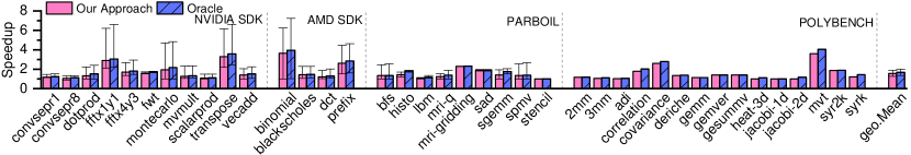
In this experiment, we exhaustively profiled each application with all possible stream configurations and report the best-found performance as the Oracle performance. The Oracle gives an indication of how close our approach is to a theoretically perfect solution. The baseline used to calculate the speedup is running the application using a single-stream without processor core or task partitioning.

The overall result is shown in Figure 9. The min-max bar on the diagram shows the range of speedups per application across all evaluated inputs. Overall, our approach achieves an average speedup of 1.57 $\times$ and 1.1 $\times$ over the single-stream configuration on XeonPhi and the GPU respectively. This translates to 93.7% and 97.9% of the Oracle performance on XeonPhi and the GPU respectively.

On XeonPhi, the performance improvement of our approach comes from two factors. First, by predicting the right processor partition size, our approach allows effective overlapping of the host-device communication and computation. Second, by matching task parallelism to the number of available processor cores, our approach can reduce the overhead of thread management, compared to the single-stream execution. When the host-device communication time dominates the streaming process, the performance improvement mainly comes from computation-communication overlapping and the speedup from streaming is consistently less than 2 $\times$ . When the kernel execution time dominates the stream process, the application can benefit from the overhead reduction of thread management. In this case, the speedup can be as large as 5 $\times$ . We provide a further discussion on this later in Section 6.5.1.

On the GPU, we can exploit bidirectional data transfer between the host and the device by using pined memory which is not supported by hStreams. The support of bidirectional data transfer allows us to obtain further performance gains by overlapping host-device data transfer and computation. The theoretically up-bound speedup on the GPU platform is 3 $\times$ , when data transfer is perfectly overlapped with computation. The representative sample is fftx4y3 with the larges dataset, the data transfer time in the two directions is the same, and the kernel execution time is 1.5 times of the data transfer time. The oracle speedup is 2.3 $\times$ , and our approach achieves a speedup of 2.2 $\times$ . On the other hand, because the current GPU implementation does not support processor core partition, the kernel execution time benefits less from using multiple streams. Programs which the kernel execution time dominated have no speedup using multiple streams, such as bfs, MonteCarlo.

6.2 Comparison to Fixed Stream Configurations

Our approach predicts from a wide range of stream configurations, which configuration is likely to give the best performance for a given program and dataset. A natural question to ask is that: is there a fixed stream configuration that gives reasonable good performance across benchmarks and datasets? To answer this question, we compare our predictive modeling based approach to two specific configurations on each of our evaluation platforms. Our justification for why we selecting the fixed configurations are described as follows. On XeonPhi, our initial results in Section 2 indicate that using the stream configuration of $(4,16)$ , i.e. partitioning the cores to 4 groups and running 4 tasks on each partition (16 tasks in total), gives good performance. The statistics obtained from the training data suggest that the configuration of $(17,85)$ give the best average performance across training samples. On the GPU, several programs support a maximum of 4 tasks. Thus we select the two configurations $(2,2)$ and $(4,4)$ . The results are shown in Figure 10.

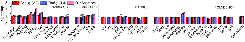
6.2.1 XeonPhi

On XeonPhi, we observe improved performance for several benchmarks such as mri-gridding, transpose, sad, under both configurations, but slower performance for dotprod, vecadd, blackscholes, lbm, and mir-q (Figure 10a). For prefix, configuration $(17,85)$ delivers improved performance while configuration $(4,16)$ leads to slowdown performance. Overall, none of the two fixed configurations give an improved performance on average. On average, our approach outperforms the two fixed configurations by a factor of 1.4, and delivers consistently improved performance across benchmarks and datasets.

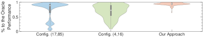
The violin plot in Figure 11a shows how far is each of the three schemes to the Oracle performance across benchmarks and datasets. Our approach not only delivers the closest performance to the Oracle, but also has the largest number of samples whose performance is next to the Oracle. By contrast, the performance given by the fixed configurations for many samples is farther from the Oracle performance.

6.2.2 GPU

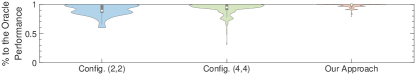
On the GPU, in most cases, the performance of configuration $(2,2)$ is moderate, not great, but not much worse than single-version, leading to an average speedup 1.03 $\times$ (Figure 10b). By contrast, although configuration $(4,4)$ performs poorly on two programs, it delivers a slightly larger averaged speedup of 1.04 $\times$ . By choosing the stream configuration on a per-program basis, our approach outperforms the two fixed configurations, achieving an averaged speedup 1.10 $\times$ . On only four programs, our approach delivers slightly worse performance with a small margin.

The violin plot in Figure 11b also confirms the strengths of our approach by presenting the distribution of performance improvement. The results on the diagram are normalized to the Oracle (best-available) performance. For most of the programs, the two fixed configurations deliver 80% to 100% to the Oracle performance. However, configuration $(4,4)$ can lead to rather poor performance (less than 40% to the best available performance) on some programs. Compared to the fixed configurations, the performance distribution given by our approach is centralized on a range between 90% to 100%, where most programs are within this percentile range. Furthermore, compared to the fixed configurations, our approach has a fewer number of performance outliers, which have less serious performance slowdown. Therefore, our approach delivers consistently better performance compared with the fixed configurations.

6.2.3 Summary

This experiment confirms that a fixed configuration fails to deliver improved performance across applications and datasets, and selecting a right stream configuration on a per program, per dataset basis is thus required.

6.3 Comparison to Analytical Models

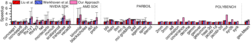
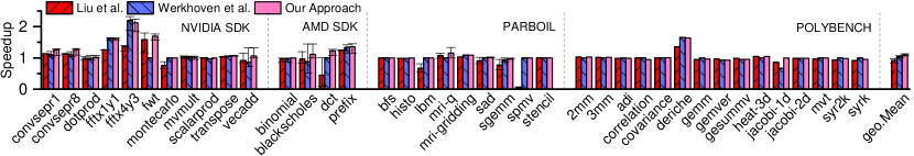
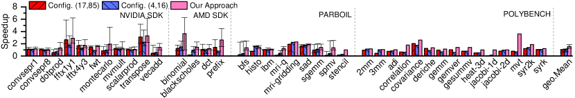
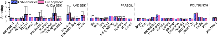
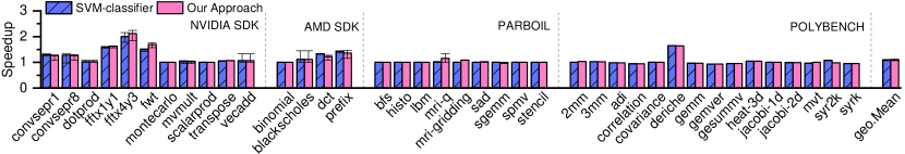
In this experiment, we compare our approach to the two recent analytical models described in Section 5.2. The results are shown in Figures 12 and 13. On XeonPhi, both competitive models prefer using $2$ tasks across benchmarks and datasets. This is because that many programs are kernel dominated, the analytical models simply assume that task partition has no effect on kernel’s performance, and do not consider the thread management overhead. On the GPU, the model proposed by Liu et al. tends to use $2$ tasks across benchmarks and datasets. This is due to the fact that most programs are data transfer dominated and this model ignores the overlap of the bidirectional data transfers between the host and the device.

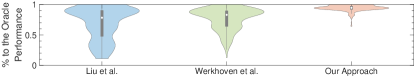
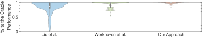
XeonPhi. Figure 12a demonstrates that our approach gives better performance for nearly all programs on XeonPhi. For the remaining handful programs, all three approaches deliver comparable performance. Compared to the results Figure 10, we can find the performance of the analytical models is similar to fixed stream configurations. This is because the performance of the seven programs, such as binomial, changes dramatically with different stream configurations (see also Figure 2). The performance of the remaining programs is not sensitive to the variation of stream configurations. From Figure 13a, we can further see that Liu et al. and Werkhoven et al. deliver a speedup within a range on 20% to 80%, while the performance of our approach is centralized on a range between 80% to 100%. Thus, our approach delivers consistently better performance compared with the alternative models.

GPU. Figure 12b shows that our approach delivers better performance for around 75% of the programs on the GPU. Since Werkhoven et al. and Liu et al. are manually tuned for the GPUs, they give better performance on some benchmarks over our approach. However, our approach has the advantages of being automatically learned from training data, with little expert involvement. The performance of our approach can be further improved by using more training examples to better cover the program space. Figure 13b shows that Liu et al. and Werkhoven et al. delivers a speedup within a range of 5% to 80%, and 70% to 100%, respectively. By contrast, the performance of our approach is centralized within a range between 90% to 100% for more programs. Therefore, overall, our approach delivers better average performance compared with the alternative models.

6.4 Comparison to Classification-based Approach

Our prior work uses a SVM classifier to predict the configurations [16]. Compared with it, the regression-based model presented in this article has several advantages.

A classification model predicts which of a set of predefined labels the input belongs to. Using this strategy, we will need to label each unique stream configuration. This will lead to a total of 175 labels for 311 profiling samples on the XeonPhi, and 11 labels on the GPU. On the XeonPhi, the ratio of samples to labels is too small to build an accurate model. As a result, we have to merge labels in our prior work [16] at the cost of losing accuracy. Classification is a constraint optimization problem where the model has to know all the possible configurations during training. Our new regression-based approach avoids this pitfall by directly modeling the impact of the stream configuration; it thereby can be used on any stream configuration as the configuration is the model’s input.

Figure 14a presents results obtained on the XeonPhi. Our regression-based approach outperforms the SVM-classifier in 21 of the 39 programs and achieves over 5% performance improvement for 13 programs. It is to note that the overhead for ranking stream configurations is included in the experimental results. Overall, our regression-based approach improves the SVM-classifier by, on average, 3% (up to 46%). Unlike XeonPhi, we were able to obtain sufficient training samples per label (because the optimization space is smaller) on the GPU to build a more accurate classification model. As can be seen from Figure 14b, the average speedup of SVM-classifier and the regression-based approach is comparable.

Compared to a classifier, our regression-based approach has the advantage of being able to be applied to configurations that were not seen during the training phase. Therefore, our approach has a better generalization ability.

6.5 Further Analysis of Performance Results

We now take a closer look into the performance results, using XeonPhi as a case study.

6.5.1 High Speedup Cases

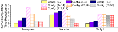
On XeonPhi, bidirectional data transfer between the host and the accelerator cannot be overlapped, i.e., we can only issue data transfer from the host to the device or vice versa at once but not simultaneously. As a result, the theoretical up-bound speedup for overlapping computation and communication is 2 $\times$ , when the computation is perfectly overlapped with the data transfer time. It is interesting to observe that several benchmarks achieve a speedup of over 2 $\times$ on XeonPhi (see Figure 9a). After having a closer investigation, we notice that such performance is attributed to the reduction in the kernel execution time in additional to the overlapping of communication and computation.

To quantify the benefit of kernel time reduction, we measure the kernel execution time with and without multiple streams and calculate the speedup between them. Note that we exclude the host-device communication time in this case to isolate the contributing factors. The kernel time improvement for transpose, binomial, and fftx1y1 is shown in Figure 15. As can be seen from the diagram, choosing a good stream configuration can lead to more than 4x reduction on the kernel execution time. This is because these benchmarks are implemented by parallelizing the inner loop within a nested loop. During runtime, the parallel threads working on the inner loop will be created, synchronized, or destroyed for each outer loop iteration. Such threading overhead could be significant when the outer loop iterates a large number of times. With multiple streams, we divide the whole outer loop iteration space into multiple smaller iterations. This allows multiple groups of threads to be managed simultaneously, leading to a significant decrease in threading overhead and faster kernel execution time. On the other hand, using too many streams and partitions will lead to a performance decrease. This is because stream management also comes at a cost, which increases as the number of partitions grows. Nonetheless, for applications where the kernel computation dominates the program execution time, by reducing the kernel time can lead to additional improvement, yielding more than 2x speedups.

6.5.2 Speedup Distribution

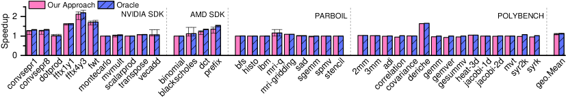
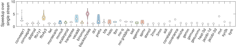
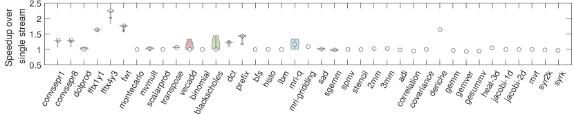
Figure 16 gives the speedup per benchmark across datasets on XeonPhi and the GPU. The shape of the violin plot corresponds to the speedup distribution.

On XeonPhi, we see that the speedups of montecarlo and prefix distribute fairly uniformly while the data distribution of fftx1y1 and fftx4y3 is multimodal (i.e. it has two peaks). Further, the input datasets have little impact on the behavior of fwt and lbm, so the speedups remain constant across datasets.

On the GPU, the speedups of dotprod, vecadd, blackscholes and mri-q distribute fairly uniformly while the data distribution of convsepr1, convsepr8, fftx1y1, fftx4y3 and dct is unimodal (i.e. it has one peak). Furthermore, the input datasets have a very slight impact on the performance behaviors of montecarlo, scalarprod, transpose and binomial. Thus, their speedups remain constant across datasets.

To conclude, the streaming speedups of some applications are sensitive to their input datasets whereas the others are not. And the distribution of speedups on the GPU is more concentrated than XeonPhi. This is because the current GPU implementation does not support processor core partition, the kernel execution time benefits less from multiple streams than XeonPhi.

6.5.3 Correlation Analysis

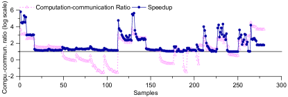
Figure 17 shows the relation between the computation-communication ratio and the achieved speedup when using heterogeneous streams across all benchmarks and datasets on XeonPhi. We see that the computation-communication ratio varies over the benchmarks and the speedup changes accordingly, but in general, a higher computation-to-communication ratio leads to a greater speedup. As explained in Section 6.5.1, in addition to overlapping computation and communication, our approach can also reduce the kernel computation time by choosing the right stream configuration. Therefore, benchmarks with a high computation-communication ratio also benefit from a reduction in the kernel computation time.

To quantify the relation between the computation-communication ratio and the speedup, we calculate the Pearson correlation coefficient of the two variables. The calculation gives a correlation coefficient of 0.7, indicating that the two variables (the computation-communication ratio and the speedup) have a strong linear correlation. By carefully selecting the stream configuration, our approach tries to maximize the overlap between communication and computation, which thus leads to favourable performance.

6.5.4 Impact of Streaming Parallelism

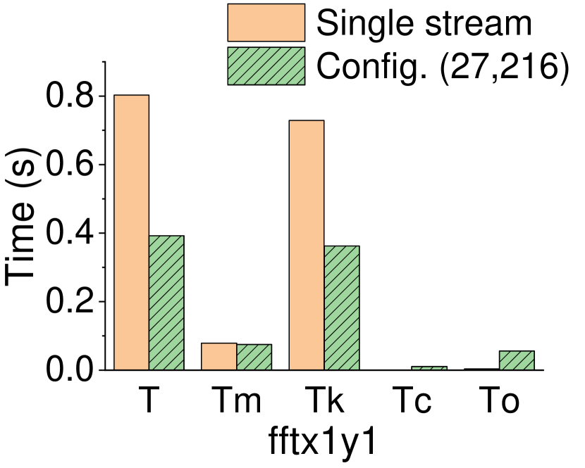
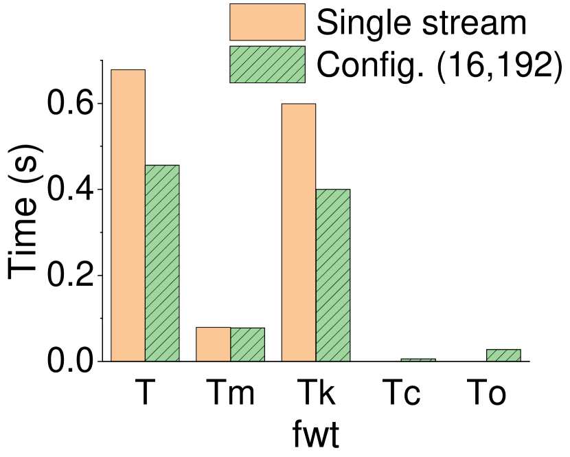
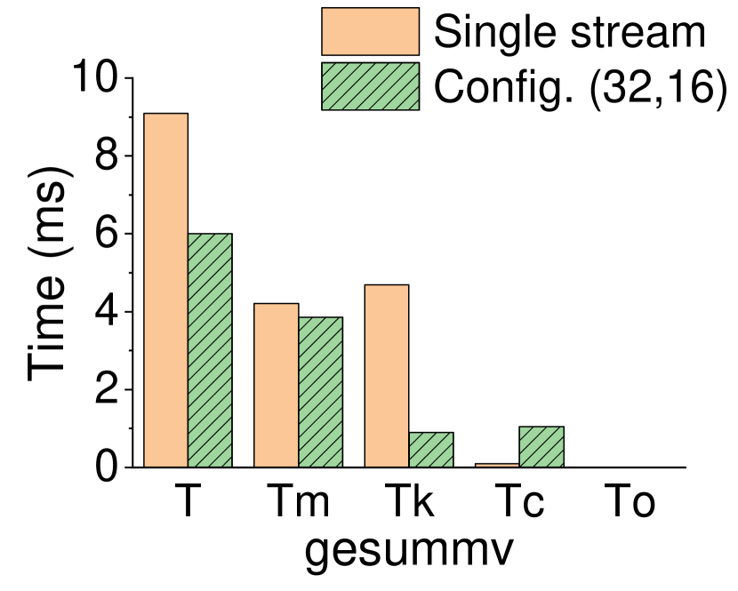
Our earlier experiments show that by carefully exploiting streaming parallelism, we can significantly improve application performance. We now take a closer look at three representative benchmarks, fftx1y1, fwt and gesummv, to get a better understanding of streaming performance on XeonPhi. These benchmarks represent different degrees of benefits obtained from streamed parallelism (with a speedup of 2 $\times$ , 1.5 $\times$ and 1 $\times$ , respectively).

We use the following analytical model to breakdown the execution time of a multi-stream program:

T=T_{m}+T_{k}+T_{c}-T_{o}

(1)

where $T_{m}$ is host-device data transfer time, $T_{k}$ is kernel execution time, $T_{c}$ is the overhead for initializing the context, and $T_{o}$ is overlapping time between data transfer and kernel execution. We measure $T$ , $T_{m}$ , $T_{k}$ , and $T_{c}$ , and use the measurements to calculate $T_{o}$ .

Figure 18 gives the breakdown for the five components in Equation 1. For each testing program, we compare the single-stream configuration against the best-performing multi-stream configuration. The host-device data transfer time, $T_{m}$ , is nearly constant among a single and a multiple stream configuration, but multi-streaming can reduce the kernel execution time, $T_{k}$ , by exploiting the spatial sharing of processing resources among computation tasks. The overhead of initializing the hStreams context, $T_{c}$ , depends on the kernel execution time. For fftx1y1 and fwt, whose kernels run for a sufficiently long time, this one-off runtime overhead is negligible. However, for gesummv, this overhead cannot be ignored due to the relatively short kernel running time. The contribution for overlapping host-device communications with kernel execution, $T_{o}$ , varies across programs. For fftx1y1 and fwt, it accounts for around 50% of $T_{m}$ , suggesting that by exploiting temporal sharing to overlap communication with kernel execution can amortize the host-device communication overhead. For gesummv, $T_{o}$ is small due to little alignment between data transfer and kernel execution. As such, there is little benefit for exploiting temporal sharing for this program.

This experiment gives a more detailed analysis for the benefits of exploiting multiple streams. The results reinforce our claim that the benefit for streaming parallelism depends on the computation kernel and hence an adaptive scheme for choosing the optimal stream configuration is needed. Our work aims to offer such a capability.

6.6 Analysis of Predictive Modeling Techniques

In this section, we analyse the working mechanism of our predictive model, using XeonPhi as an evaluation platform.

6.6.1 Comparison to Alternative Modeling Techniques

We compare our MLP-based model against four widely used regression methods: the DCT (Decision Tree), the RF (Random Forest), the XGB (eXtreme Gradient Boosting) and SVM (Support Vector Machine) as well as four classification models: SVM, DCT, MLP and KNN (K-Nearest Neighbors). We use the Radial basis function kernel for the SVM models.

For each technique, we follow the same training methodology and use the same features and training examples to build a model. For classification models, we apply the label merging process described in our prior work [16] to improve the prediction accuracy. Table V compares the training overhead, average prediction time and achieved average speedup for each model. We note that training a regression-based SVM model has the largest overhead. Although training a DCT has less overhead over our MLP-based regression model, MLP gives better prediction performance. The RF and XGB models are based on DCT, but they do not yield a better performance. Compared to regression models, a classification model takes less time to train and make predictions. However, classification models give worse performance over regression models as they require more training data to cover the optimization space. Overall, we choose to use a regression-based approach and employ MLP because it gives the best overall prediction performance and has modest training overhead.

Table V: Comparison to alternative modeling techniques

Technique	Training time	Avg. pred. time	Avg. speedup
SVM (regression)	100 hours	2280 ms	1.56
DCT (regression)	65.57 seconds	0.74 ms	1.51
RF (regression)	317.89 seconds	11.94 ms	1.51
XGB (regression)	28.46 seconds	0.74 ms	1.49
MLP (regression, ours)	245.8 seconds	0.76 ms	1.57
SVM (classifier)	1.28 seconds	0.10 ms	1.53
DCT (classifier)	0.79 seconds	0.05 ms	1.38
MLP(classifier)	46.45 seconds	0.05 ms	1.41
KNN (classifier)	0.22 seconds	0.23 ms	1.43

6.6.2 Feature Engineering

Feature engineering has a significant impact on the performance of a machine learning model (Section 3.2). Here we quantify the impact of feature engineering methods. In this work, we consider three standard feature engineering approaches including standardization, normalization and dimension reduction.

Standardization converts all features value to be in a common range, e.g., between 0 and 1. The idea is to prevent the feature value range to dominate the importance of that feature. In this work we apply a commonly used standardization method called Z-score [29] to standardize the raw feature values and the speedups (i.e., prediction targets) in the training data. We found that feature standardization improves the achieved speedup by 3% on average, and speedup standardization improves the achieved speedup by 5% on average.

Normalization scales the feature values to make them follow the normal distribution. We have tested a range of normalization methods including the square root, the reciprocal of square root and the natural logarithm transformation. However, we found that normalization does not improve our model prediction accuracy.

Dimension reduction reduces the number of features, which is often useful when the number of training examples is not proportional to the number of feature dimensions. In this work, we apply factor analysis (FA) [30] and principal component analysis (PCA) [31] to the raw features. Applying PCA and using 9 PCA components gives the best overall result, by improving the average speedup by 17%. PCA outperforms FA which gives an average 3% improvement on the achieved speedup.

6.6.3 MLP Parameters Tuning

We now discuss the impact of the MLP parameter choices. There are four configurable parameters for an MLP model: the activation function, the number of hidden layers, the number of neurons, and the learning algorithm (i.e., the solver). For activation functions, we consider identity, logistic, tanh and relu. For hidden layers and neurons, we vary the number of hidden layers from 1 to 5 and the number of neurons per layer from 3 to 100. For the solver, we consider three commonly used weight optimizers: lbfgs, sgd and and adam. We use scikit-learn implementations for the activation function and the solver. Our experimental results suggest that the best-performing activation function and solver are tanh and adam respectively, and using three hidden layers with 9 neurons per layers gives the best overall results on our training data. Overall, tuning MLP model parameter improves the average speedup by 5% over the default parameter setting.

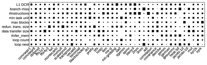
6.6.4 Impact of Individual Feature

In this experiment, we consider the impact of a specific feature to the resultant performance. Figure 19 presents a Hinton diagram illustrating how important a feature contribution to the performance model prediction accuracy (which in turns affects the resulting application performance). The larger the box, the more significant a feature for a given program’s performance. Here, the x-axis denotes the programs, and the y-axis denotes the features used by our performance model. The impact of a feature is quantified by measuring how much speedup improvement can be obtained if that feature is used by the performance model. Note that this is a post-hoc analysis and, in general, we cannot know in advance the importance of a feature on unseen programs. Figure 19 shows that all the features are important for the set of benchmarks targeted in the work, but the importance of features varies across programs. This diagram illustrates how hard it is to develop an analytical model to capture the diverse behaviors and characteristics of streaming programs.

7 Related Work

Our work builds upon the following past foundation, while qualitatively differing from each.

Task Scheduling. There is considerable work on distributing work across heterogeneous processors to improve application performance [32, 33, 34]. Prior work in the area typically assumes that the processor configuration is fixed and relies on the operating system to schedule parallel tasks across processing units. Recent studies show that by partitioning the processing units into groups it is possible to significantly improve the application performance by overlapping the host-device communication and computation on coprocessors like Intel XeonPhi [14, 6]. However, existing approaches rely on static tuning to find the processor partition and the best number of streams to run within a partition. As a result, previous approaches cannot adapt to the change of program inputs. As a departure from prior work, we develop an automatic approach to dynamically adjust the processor partition and task-granularity during runtime, considering the characteristics of applications and input datasets; our approach thereby can adapt to the change of program inputs.

Domain-specific Optimizations There is considerable work on domain-specific optimization on Intel XeonPhi. Cheng et al. [35] and Jha et al. [36] show that in-memory database applications suffer from under-utilization of processor resources and hence a fine-grained tuning approach is required. Mrphi is a framework for optimizing MapReduce workload on the XeonPhi [37]. It employs a set of techniques to improve the resource utilization to obtain higher application performance. Other works look at performance optimization for numerical solvers [38], sparse matrix vector multiplication [39, 40], and dynamic stochastic economic models [39]. Ferrão et al. [41] and Memeti et al. [42] develop a stream processing framework for XeonPhi to increase the programming productivity. The runtime can automatically distribute workloads across CPUs and accelerating devices. These approaches improve the processor utilization by adjusting the algorithmic design, which are complementary to our work on tuning multi-streaming parallelism for data parallel applications.

Multiple Streams Modeling. Gomez-Luna et al. [11] develop a set of models to estimate the asynchronous data transfer overhead on different GPU architectures. The models can be used to estimate the optimal number of streams to use on a given GPU platform. Werkhoven et al. [10] present an analytical model to determine when to apply an overlapping method on GPUs. Liu et al. [12] also develop an analytical based approach to determine the optimal number of streams to use on GPUs. However, none of these approaches considers the processor partition. As we have shown in Section 6.3, ignoring the processor partitioning parameter can lead to poor performance on Intel XeonPhi. Furthermore, these hand-crafted models have the drawback of being not portable across architectures as the model is tightly coupled to a specific GPU architecture. Our work advances prior work by employing machine learning to automatically learn the optimal processor partition and the number of streams/tasks to use. Since our models are automatically learned from empirical observations, one can easily re-learn a model for a new architecture.

Predictive Modeling. Recent studies have shown that machine learning based predictive modeling is effective in code optimization [43, 44], performance predicting [45, 46], parallelism mapping [47, 48, 20, 49, 50], and task scheduling [51, 52, 53, 54, 55, 56]. Its great advantage is its ability to adapt to the ever-changing platforms as it has no prior assumption about their behavior. The work presented by Wen et al. [57] employs SVMs to develop a binary classifier to predict that if a given OpenCL kernel can achieve a large speedup or not. Our work differs from [57] in that it targets a different architecture and programming model, and it predicts from a larger number of configurations instead of making a binary prediction. Our prior work developed an SVM based classifier to predict the optimal stream configuration for Intel XeonPhi [16]. However, it requires having sufficient training data samples to cover all possible stream configurations. Our approach improves the prior work by directly modeling the impact of the stream configuration. As a result, our approach can make predictions for any stream configuration (even those are not seen in the training data).

Autotuning Parallel Programs. Our approach is closely related to autotuning that searches for the best-performing optimization configuration [58, 59]. This technique is demonstrated to be effective for choosing algorithmic choices [60], tuning GPU code [61, 62, 63], optimizing structured parallel programs [64, 65, 66] and non-uniform memory access (NUMA) architectures [67], and more recently for deep neural networks [68]. Many of the prior works in this area employ an evolutionary-based approach by applying and profiling candidate optimization options to choose a good option to use. One of the key changes of autotuning is how to avoid the profiling overhead which could be prohibitively expensive. We do so by using a performance model to quickly evaluate the profitability of a candidate optimization option. We show that our approach has low runtime overhead, which thus permits us to apply it at runtime to best match the optimization strategy to the program input. Furthermore, our work is the first for tuning heterogeneous streaming parallelism on heterogeneous many-cores (XeonPhis and GPUs).

Automatic Generation of Parallel Programs. The OpenMPC compiler [69] translates OpenMP to CUDA programs. Wang et al. [24, 20, 70] translates OpenMP to OpenCL programs and use machine learning to select the most suitable device from the host CPU and the GPU to run the code. Rawat et al. presents an automatic approach to generate GPU code from a domain-specific language (DSL) for stencil programs [71]. All of the above approaches target GPUs, and do not utilize the multi-streaming strategy.

8 Conclusion

This article has presented an automatic approach to exploit streaming parallelism on heterogeneous many-cores. Central to our approach is a machine learning-based model that predicts the resulting performance when running the target application under a given streamed configuration. The performance predictor is then used as a cost function to quickly rank candidate configurations at runtime, to determine which stream configuration should be used on a per-program per-dataset basis. We have evaluated our approach on an Intel XeonPhi and an NVIDIA GTX 1080 Ti GPU, with 39 representative benchmarks. Experimental results show that our approach delivers an average speedup of 1.6x and 1.1x on XeonPhi and the GPU, respectively. These results translate to over 93% of the best-available performance.

Acknowledgment

This work was partially funded by the National Key Research and Development Program of China under Grant No. 2018YFB0204301, the National Natural Science Foundation of China under Grant agreements 61972408, 61602501 and 61872294; For any correspondence, please contact Jianbin Fang (Email: j.fang@nudt.edu.cn).

References

[1] J. D. Owens et al., “Gpu computing,” Proceedings of the IEEE, 2008.
[2] A. Li et al., “Exploring and analyzing the real impact of modern on-package memory on HPC scientific kernels,” in SC, 2017.
[3] C. Chen et al., “LU factorization on heterogeneous systems: an energy-efficient approach towards high performance,” Computing, 2017.
[4] M. R. Meswani et al., “Modeling and predicting performance of high performance computing applications on hardware accelerators,” IJHPCA, 2013.
[5] J. Fang et al., “A comprehensive performance comparison of CUDA and opencl,” in ICPP, 2011.
[6] C. J. Newburn, et al., “Heterogeneous streaming,” in IPDPSW, 2016.
[7] CUDA C Best Practices Guide Version 7.0, NVIDIA Inc., 2015.
[8] The Khronos OpenCL Working Group, “OpenCL - The open standard for parallel programming of heterogeneous systems,” http://www.khronos.org/opencl/, 2016.
[9] hStreams Architecture for MPSS 3.5, Intel Inc., 2015.
[10] B. Van Werkhoven et al., “Performance models for cpu-gpu data transfers,” in CCGrid, 2014.
[11] J. GóMez-Luna et al., “Performance models for asynchronous data transfers on consumer graphics processing units,” JPDC, 2012.
[12] B. Liu et al., “Software pipelining for graphic processing unit acceleration: Partition, scheduling and granularity,” IJHPCA, 2016.
[13] Z. Li et al., “Streaming applications on heterogeneous platforms,” in NPC, 2016.
[14] J. Fang et al., “Evaluating multiple streams on heterogeneous platforms,” Parallel Processing Letters, 2016.
[15] Z. Li et al., “Evaluating the performance impact of multiple streams on the mic-based heterogeneous platform,” in IPDPSW, 2016.
[16] P. Zhang et al., “Auto-tuning streamed applications on intel xeon phi,” in IPDPS, 2018.
[17] C. Lattner and V. Adve, “LLVM: A compilation framework for lifelong program analysis & transformation,” in CGO, 2004.
[18] F. Pedregosa et al., “Scikit-learn: Machine learning in python,” Journal of machine learning research, 2011.
[19] G. Fursin et al., “Milepost gcc: machine learning based research compiler,” in GCC summit, 2008.
[20] Z. Wang et al., “Automatic and portable mapping of data parallel programs to opencl for gpu-based heterogeneous systems,” ACM TACO, 2015.
[21] S. Boslaugh, Statistics in a Nutshell, 2nd Edition, 2nd ed. O’Reilly Media, 2012.
[22] B. F. Manly, Multivariate statistical methods: a primer. CRC Press, 2004.
[23] S. Lee et al., “Openmp to gpgpu: a compiler framework for automatic translation and optimization,” ACM Sigplan Notices, 2009.
[24] D. Grewe et al., “Portable mapping of data parallel programs to opencl for heterogeneous systems,” in CGO, 2013.
[25] D. Mikushin et al., “Kernelgen–the design and implementation of a next generation compiler platform for accelerating numerical models on gpus,” in IPDSW, 2014.
[26] T. Grosser and T. Hoefler, “Polly-acc transparent compilation to heterogeneous hardware,” in Supercomputing, 2016.
[27] R. Sotomayor et al., “Automatic cpu/gpu generation of multi-versioned opencl kernels for c++ scientific applications,” International Journal of Parallel Programming, 2017.
[28] W. Ertel, “On the definition of speedup,” in International Conference on Parallel Architectures and Languages Europe, 1994.
[29] E. Kreyszig, Advanced Engineering Mathematics, 10th Eddition, 2009.
[30] R. L. Gorsuch, Factor Analysis, 2nd Edition. Routledge, 2014.
[31] H. Hotelling, “Analysis of a complex of statistical variables into principal components.” Journal of educational psychology, 1933.
[32] S. Mittal and J. S. Vetter, “A survey of CPU-GPU heterogeneous computing techniques,” ACM Computing Surveys (CSUR), vol. 47, no. 4, p. 69, 2015.
[33] C.-K. Luk et al., “Qilin: exploiting parallelism on heterogeneous multiprocessors with adaptive mapping,” in MICRO, 2009.
[34] J. Shen et al., “Workload partitioning for accelerating applications on heterogeneous platforms,” IEEE TPDS, 2016.
[35] X. Cheng et al., “Many-core needs fine-grained scheduling: A case study of query processing on intel xeon phi processors,” JPDC, 2018.
[36] S. Jha et al., “Improving main memory hash joins on intel xeon phi processors: An experimental approach,” PVLDB, 2015.
[37] M. Lu et al., “Mrphi: An optimized mapreduce framework on intel xeon phi coprocessors,” IEEE TPDS, 2015.
[38] A. Lastovetsky et al., “Model-based optimization of eulag kernel on intel xeon phi through load imbalancing,” IEEE TPDS, 2017.
[39] W. T. Tang et al., “Optimizing and auto-tuning scale-free sparse matrix-vector multiplication on intel xeon phi,” in CGO, 2015.
[40] M. E. Guney et al., “Optimizing matrix multiplication on intel® xeon phi th x200 architecture,” in ARITH, 2017.
[41] P. Ferrão et al., “Stream processing on hybrid cpu/intel® xeon phi systems,” in European Conference on Parallel Processing, 2018.
[42] S. Memeti and S. Pllana, “Hstream: A directive-based language extension for heterogeneous stream computing,” in CSE, 2018.
[43] C. Cummins et al., “End-to-end deep learning of optimization heuristics,” in PACT, 2017.
[44] Z. Wang and M. O’Boyle, “Machine learning in compiler optimisation,” Proc. IEEE, 2018.
[45] J. Zhao et al., “Predicting cross-core performance interference on multicore processors with regression analysis,” IEEE TPDS, 2016.
[46] Z. Wang and M. F. O’boyle, “Using machine learning to partition streaming programs,” ACM TACO, 2013.
[47] G. Tournavitis et al., “Towards a holistic approach to auto-parallelization: integrating profile-driven parallelism detection and machine-learning based mapping,” ACM Sigplan Notices, 2009.
[48] Z. Wang and M. F. O’Boyle, “Partitioning streaming parallelism for multi-cores: a machine learning based approach,” in PACT, 2010.
[49] Z. Wang et al., “Integrating profile-driven parallelism detection and machine-learning-based mapping,” ACM TACO, 2014.
[50] B. Taylor et al., “Adaptive optimization for opencl programs on embedded heterogeneous systems,” in LCTES, 2017.
[51] M. K. Emani et al., “Smart, adaptive mapping of parallelism in the presence of external workload,” in CGO, 2013.
[52] V. S. Marco et al., “Improving spark application throughput via memory aware task co-location: A mixture of experts approach,” in Middleware, 2017.
[53] J. Ren et al., “Optimise web browsing on heterogeneous mobile platforms: a machine learning based approach,” in INFOCOM, 2017.
[54] ——, “Proteus: Network-aware web browsing on heterogeneous mobile systems,” in CoNEXT ’18, 2018.
[55] L. Yuan et al., “Using machine learning to optimize web interactions on heterogeneous mobile systems,” IEEE Access, 2019.
[56] B. Taylor et al., “Adaptive deep learning model selection on embedded systems,” ACM SIGPLAN Notices, 2018.
[57] Y. Wen et al., “Smart multi-task scheduling for opencl programs on cpu/gpu heterogeneous platforms,” in HiPC, 2014.
[58] K. Datta et al., “Stencil computation optimization and auto-tuning on state-of-the-art multicore architectures,” in Supercomputing, 2008.
[59] J. Ansel et al., “Opentuner: An extensible framework for program autotuning,” in PACT, 2014.
[60] J. Ragan-Kelley et al., “Halide: A language and compiler for optimizing parallelism, locality, and recomputation in image processing pipelines,” in PLDI, 2013.
[61] A. Nukada and S. Matsuoka, “Auto-tuning 3-d fft library for cuda gpus,” in SC, 2009.
[62] P. Tillet and D. Cox, “Input-aware auto-tuning of compute-bound hpc kernels,” in SC, 2017.
[63] T. T. Dao and J. Lee, “An auto-tuner for opencl work-group size on gpus,” IEEE TPDS, 2018.
[64] U. Dastgeer et al., “Auto-tuning skepu: a multi-backend skeleton programming framework for multi-gpu systems,” in IWMSE, 2011.
[65] J. J. Thiagarajan et al., “Bootstrapping parameter space exploration for fast tuning,” in Supercomputing, 2018.
[66] D. Chen et al., “Optimizing sparse matrix–vector multiplications on an armv8-based many-core architecture,” International Journal of Parallel Programming, 2019.
[67] T. Katagiri et al., “Auto-tuning on numa and many-core environments with an fdm code,” in IPDPSW, 2017.
[68] L. Liao et al., “Uhcl-darknet: An opencl-based deep neural network framework for heterogeneous multi-/many-core clusters,” in ICPP, 2018.
[69] S. Lee and R. Eigenmann, “Openmpc: Extended openmp programming and tuning for gpus,” in SC, 2010.
[70] Z. Wang et al., “Exploitation of gpus for the parallelisation of probably parallel legacy code,” in CC ’14, 2014.
[71] P. S. Rawat et al., “Domain-specific optimization and generation of high-performance gpu code for stencil computations,” Proceedings of the IEEE, 2018.