Variational Inference for Deep Probabilistic Canonical Correlation Analysis

Abstract

In this paper, we propose a deep probabilistic multi-view model that is composed of a linear multi-view layer based on probabilistic canonical correlation analysis (CCA) description in the latent space together with deep generative networks as observation models. The network is designed to decompose the variations of all views into a shared latent representation and a set of view-specific components where the shared latent representation is intended to describe the common underlying sources of variation among the views. An efficient variational inference procedure is developed that approximates the posterior distributions of the latent probabilistic multi-view layer while taking into account the solution of probabilistic CCA. A generalization to models with arbitrary number of views is also proposed. The empirical studies confirm that the proposed deep generative multi-view model can successfully extend deep variational inference to multi-view learning while it efficiently integrates the relationship between multiple views to alleviate the difficulty of learning.

1 Introduction

When observations consist of multiple views or modalities of the same underlying source of variation, a learning algorithm should efficiently account for the complementary information to alleviate learning difficulty (Chaudhuri et al., 2009) and improve accuracy. A well-established method for two-view analysis is given by canonical correlation analysis (CCA) (Hotelling, 1992), a classical subspace learning technique that extracts the common information between two multivariate random variables by projecting them onto a subspace. CCA, as a standard model for unsupervised two-view learning, has been used in a broad range of tasks such as dimensionality reduction, visualization and time series analysis (Xia et al., 2014).

The goal of representation learning is to capture the essence of data and extract its natural features. Such features can be categories or cluster memberships. In multi-view data, the relationship between different views should be leveraged by the representation learning algorithms to enhance feature extraction. Learning representations in real-world applications, where the data is typically high-dimensional with complex structure, poses significant challenges and necessitates flexible and expressive yet scalable models such as deep generative neural networks to be applied.

It has been shown in (Chaudhuri et al., 2009) that by projecting multi-view data onto low-dimensional subspaces using CCA, cluster memberships can be recovered under a weak separation condition thus resulting in easier clustering in the subspace. Nevertheless, CCA exhibits poor generalization when trained on small training sets, therefore (Klami and Kaski, 2007; Klami et al., 2013) adopts a Bayesian approach to solve a probabilistic interpretation of CCA. However, real applications involve nonlinear subspaces where more than two view are available. Recently, deep learning has received renewed interest as a standard approach for describing highly expressive models for increasingly complex datasets. In multi-view learning, several deep learning based approaches have been successfully extended (Ngiam et al., 2011; Andrew et al., 2013; Wang et al., 2015; Tang et al., 2017; Abavisani and Patel, 2018a).

Main contributions: In this work, we present a modified formulation of probabilistic CCA that enables an extension to deep generative models. Generalizing the approach to an arbitrary number of views is also discussed. In this approach, linear probabilistic layers are extended to deep generative multi-view networks that capture the variations of the views by a shared latent representation that describes most of the variability (essence) of multi-view data, and a set of view-specific factors. Variational inference provides a powerful tool for scaling probabilistic models to complex problems and large scale datasets (Rezende et al., 2014; Kingma and Welling, 2013; Rezende and Mohamed, 2015). Hence, to design a scalable training algorithm, we follow variational inference principles, taking into account the probabilistic CCA formulation to achieve an approximate posterior for the latent linear multi-view layer. Empirical studies confirm that the proposed deep generative multi-view model can efficiently integrate the relationship between multiple views to alleviate learning difficulty, which is the goal of multi-view learning approaches (Chaudhuri et al., 2009).

Notation and Definitions

Throughout the paper, bold lowercase variables denote vectors (e.g. ${\bm{x}}$) or vector-valued random variables (e.g. ${\mathbf{x}}$), bold uppercase are used for matrices (e.g. ${\bm{X}}$) or matrix-valued random variables (e.g. ${\mathbf{X}}$) and unbold lowercase are scalars (e.g. $x$) or random variables (e.g. x). The transpose of a matrix is denoted as ${\bm{A}}^{\top}$ and ${\bm{e}}^{(i)}=[0,\dots,0,1,0,\dots,0]$ is the standard basis vector with a 1 at $i$th position. There are $M$ views in total and subscripts are intended to identify the view-specific variable, (e.g. ${\mathbf{x}}_{m},{\bm{\Sigma}}_{mm}$), which is different from an element of a vector that is specified by subscript (e.g. ${\textnormal{x}}_{mi}$). The difference should be clear from context.

2 Probabilistic CCA

Canonical correlation analysis (CCA) (Hotelling, 1992) is a classical subspace learning method that extracts information from the cross-correlation between two variables. Let ${\mathbf{z}}_{1}\in\mathbb{R}^{d_{1}}$ and ${\mathbf{z}}_{2}\in\mathbb{R}^{d_{2}}$ be a pair of random vectors corresponding to two different views. CCA linearly projects these onto the subspace $\mathbb{R}^{d_{0}}$ as ${\mathbf{r}}_{1}={\bm{U}}_{1}^{\top}\mathbf{z}_{1}$ and ${\mathbf{r}}_{2}={\bm{U}}_{2}^{\top}\mathbf{z}_{2}$, where ${\bm{U}}_{1}\in\mathbb{R}^{d_{1}\times d_{0}}$ and ${\bm{U}}_{2}\in\mathbb{R}^{d_{2}\times d_{0}}$ and $0<d_{0}\leq\min\{d_{1},d2\}$, such that each pair of components $({\mathbf{r}}_{1}(i),{\mathbf{r}}_{2}(j))$ are maximally correlated if $i=j$ and uncorrelated otherwise. Let $({\bm{\mu}}_{1},{\bm{\Sigma}}_{11})$ and $({\bm{\mu}}_{2},{\bm{\Sigma}}_{22})$ be the mean and covariance matrices of ${\mathbf{z}}_{1}$ and ${\mathbf{z}}_{2}$, respectively, and ${\bm{\Sigma}}_{12}$ is their cross-covariance. Then CCA can be formulated as the optimization problem

$$\max_{{\bm{U}}_{1},{\bm{U}}_{2}}\mathop{\mathrm{tr}}[{\bm{U}}_{1}^{\top}{\bm{\Sigma}}_{12}{\bm{U}}_{2}]$$ (1)

$${\bm{U}}_{1}^{\top}{\bm{\Sigma}}_{11}{\bm{U}}_{1}={\bm{U}}_{2}^{\top}{\bm{\Sigma}}_{22}{\bm{U}}_{2}=\mathbf{I}_{d_{0}}$$

Given $({\bm{v}}_{1i},{\bm{v}}_{2i}),~{}i\in[1,...,d_{0}]$ as the pairs of left and right singular vectors corresponding to $d_{0}$ largest singular values, $p_{i}~{}i\in[1,...,d_{0}]$, of the correlation matrix ${\bm{\Sigma}}_{11}^{-1/2}{\bm{\Sigma}}_{12}{\bm{\Sigma}}_{22}^{-1/2}$, the solution to the CCA problem is given by $({\bm{u}}_{1i},{\bm{u}}_{2i})=({\bm{\Sigma}}_{11}^{-1/2}{\bm{v}}_{1i},{\bm{\Sigma}}_{22}^{-1/2}{\bm{v}}_{2i}),~{}i\in[1,...,d_{0}]$ where $({\bm{u}}_{1i},{\bm{u}}_{2i})$, also called canonical pairs of directions, form the columns of $({\bm{U}}_{1},{\bm{U}}_{2})$ and ${\bm{P}}_{d_{0}}=\text{diag}([p_{0},...,p_{d_{0}}])$ is the diagonal matrix of canonical correlations.

Bach and Jordan (2005) and Browne (1979) proposed a probabilistic generative interpretation to the classical CCA problem that reveals the shared latent representation explicitly. An extension of their results to a more flexible model can be expressed as follows.

Figure 1: Graphical representation of the deep probabilistic CCA model, where the blue edges belong to latent linear probabilistic CCA model and the black edges represent the deep nonlinear observation networks (decoders) $p_{\theta_{m}}({\mathbf{x}}_{m}|{\mathbf{z}}_{m})=g_{m}({\mathbf{z}}_{m};\theta_{m})$. Shaded nodes denotes observed views and dashed line represent the stochastic samples drawn from the approximate posteriors.

Theorem 1

Assume the probabilistic generative model for the graphical model in Figure 1 as:

$$\bm{\phi} \sim\mathcal{N}({\bm{\mu}}_{0},\mathbf{I}_{d_{0}}),\quad 0<d_{0}\leq\min\{d_{1},d_{2}\}$$ (2)

$${\mathbf{z}}_{1}|\bm{\phi} \sim\mathcal{N}({\bm{W}}_{1}\bm{\phi}+{\bm{\mu}}_{{\epsilon}_{1}},{\bm{\Psi}}_{1}),\quad{\bm{W}}_{1}\in\mathbb{R}^{d_{1}\times d_{0}},{\bm{\Psi}}_{1}\succcurlyeq 0$$

$${\mathbf{z}}_{2}|\bm{\phi} \sim\mathcal{N}({\bm{W}}_{2}\bm{\phi}+{\bm{\mu}}_{{\epsilon}_{2}},{\bm{\Psi}}_{2}),\quad{\bm{W}}_{2}\in\mathbb{R}^{d_{2}\times d_{0}},{\bm{\Psi}}_{2}\succcurlyeq 0$$

where $\bm{\phi}$ is the shared latent representation. The maximum likelihood estimate of the parameters of this model can be expressed in terms of the canonical correlation directions as

$$\hat{{\bm{W}}}_{1} ={\bm{\Sigma}}_{11}{\bm{U}}_{1}{\bm{M}}_{1}$$ (3)

$$\hat{{\bm{W}}}_{2} ={\bm{\Sigma}}_{22}{\bm{U}}_{2}{\bm{M}}_{2}$$

$$\hat{{\bm{\Psi}}}_{1} ={\bm{\Sigma}}_{11}-\hat{{\bm{W}}}_{1}\hat{{\bm{W}}}_{1}^{\top}$$

$$\hat{{\bm{\Psi}}}_{2} ={\bm{\Sigma}}_{22}-\hat{{\bm{W}}}_{2}\hat{{\bm{W}}}_{2}^{\top}$$

$$\hat{{\bm{\mu}}}_{{\epsilon}_{1}} ={\bm{\mu}}_{1}-\hat{{\bm{W}}}_{1}{\bm{\mu}}_{0}$$

$$\hat{{\bm{\mu}}}_{{\epsilon}_{2}} ={\bm{\mu}}_{2}-\hat{{\bm{W}}}_{2}{\bm{\mu}}_{0}$$

where ${\bm{M}}_{1},{\bm{M}}_{2}\in\mathbb{R}^{d_{0}\times d_{0}}$ are arbitrary matrices with spectral norms smaller than one that satisfy ${\bm{M}}_{1}{\bm{M}}_{2}^{\top}={\bm{P}}_{d_{0}}$, and the residual errors terms can be defined as ${\bm{\epsilon}}_{1}:={\mathbf{z}}_{1}-{\bm{W}}_{1}\bm{\phi}$ and ${\bm{\epsilon}}_{2}:={\mathbf{z}}_{2}-{\bm{W}}_{2}\bm{\phi}$. This probabilistic graphical model induces conditional independence of ${\mathbf{z}}_{1}$ and ${\mathbf{z}}_{2}$ given $\bm{\phi}$. The parameter ${\bm{\mu}}_{0}$ is not identifiable by maximum likelihood.

Proof:  See Appendix A. $\hbox{}\hfill\blacksquare$

In contrast to the results in (Bach and Jordan, 2005) where ${\bm{\mu}}_{0}=\mathbf{0}$, here we introduce ${\bm{\mu}}_{0}$ as an extra degree of freedom. We will see in the following the important role of this parameter in optimizing the upper bound on the likelihood, and also in the inference of the shared representation of deep probabilistic CCA. We will also derive an analytical form to identify it based on the parameters of the probabilistic multi-view layer, and develop an identification method for the arbitrary matrices ${\bm{M}}_{1},{\bm{M}}_{2}$.

2.1 Generalization to arbitrary number of views

As an extension to an arbitrary number of views for probabilistic CCA, (Archambeau and Bach, 2009) proposed a general probabilistic model as follows:

$${\mathbf{z}}_{m} ={\bm{W}}_{m}\bm{\phi}_{0}+{\bm{V}}_{m}\bm{\phi}_{m}+{\bm{\mu}}_{m}+\nu_{m},$$ (4)

$$\nu_{m} \sim\mathcal{N}(\mathbf{\bm{0}},\tau_{m}^{-1}\mathbf{I}_{d_{m}}),$$

$$\quad{\bm{W}}_{m}\in\mathbb{R}^{d_{m}\times d_{0}},{\bm{V}}_{m}\in\mathbb{R}^{d_{m}\times q_{m}},\forall m\in\{1,...,M\}$$

where $\{{\bm{\mu}}_{m}\}_{m=1}^{M}$ and $\{\nu_{m}\}_{m=1}^{M}$ are the view specific offsets and residual errors, respectively. This model can also be viewed as multibattery factor analysis (MBFA) (Klami et al., 2014; Browne, 1980) in the statistics literature, which describes the statistical dependence between all the views by a single latent vector, $\bm{\phi}_{0}$, and explains away the view-specific variations by factors private to each view. Moreover, limiting to single view, if the prior on the view-specific factor is multivariate independent Gaussian, this model includes the probabilistic factor analysis as a special case, and also reduces to probabilistic PCA given the prior is isotropic as well. Archambeau and Bach (2009) followed a Bayesian approach to the linear generative model (4) and proposed a variational Expectation-Maximization algorithm to estimate the model parameters.

A reformulation for the parameters of this general model inspired by the maximum likelihood solutions of probabilistic CCA in Theorem 1 is presented in Appendix B.

Although constraining the observation models to the classical linear model (2) offers closed form inference for the latent variable(s) and efficient training algorithms the resulting power is very limited in modeling increasingly complex data distribution. On the other hand, the generative descriptions of the probabilistic models in general, and the probabilistic multi-view models (2) and (4) in particular, can be extended naturally as the building blocks of more complex hierarchical models (Klami et al., 2013). A well established method to increase the capacity and improve the expressiveness of such models is using deep neural networks to capture nonlinear and complex structures in data distribution, therefore one can append deep generative networks on top of the linear probabilistic model to obtain a combined model denoted in this work as deep probabilistic CCA or deep probabilistic multi-view network in general. A graphical representation of this model is depicted in Figure 1. Let ${\mathbf{x}}:=\{{\mathbf{x}}_{m}\in\mathbb{R}^{d^{\prime}_{m}}\}_{m=1}^{M}$ denote the collection of observations of all views and ${\mathbf{z}}:=\{\bm{\phi}\in\mathbb{R}^{d_{0}}\}\cup\{{\mathbf{z}}_{m}\in\mathbb{R}^{d_{m}}\}_{m=1}^{M}$ be the collection of the shared latent representation and latent variables corresponding to each view. The latent linear probabilistic CCA layer of the form presented in (2) models the linear cross-correlation between all latent variables $\{{\mathbf{z}}_{m}\}_{m=1}^{M}$ in the latent space while the nonlinear generative observation networks, also called the decoders in the context of variational auto-encoders, are responsible for expressing the complex variations of each view. The observation models are described by deep neural networks $p_{\theta_{m}}({\mathbf{x}}_{m}|{\mathbf{z}}_{m})=g_{m}({\mathbf{z}}_{m};\theta_{m})$ with the set of model parameters $\theta=\{\theta_{m}\}_{m=1}^{M}$. In the following, an approximate variational inference approach is presented for training of this deep generative multi-view model.

2.2 Variational inference

To obtain the maximum likelihood estimate of the model parameters, it is desirable to maximize the marginal data log-likelihood averaged on the dataset $\mathcal{D}=\{x^{(i)}\},~{}i=1,..,N$

$$\log p_{\theta}({\mathbf{X}})=\frac{1}{N}\sum_{i=1}^{N}\log p_{\theta}({\bm{x}}^{(i)}) \simeq\mathbb{E}_{{\mathbf{x}}\sim\hat{P}_{data}}[\log p_{\theta}({\mathbf{x}})]$$

This objective requires marginalization over all the latent variables which entails the expectation of likelihood function $p_{\theta}({\mathbf{x}}|{\mathbf{z}})$ over the prior distribution of the set of latent variables, $p({\mathbf{z}})$. The marginalization is typically intractable for flexible models, hence, one work around is to follow the variational inference principle (Jordan et al., 1999), by introducing an approximate posterior distribution $q_{\eta}({\mathbf{z}}|{\mathbf{x}})$ — also known as variational inference network in the context of amortized variational inference — and maximize a resulting variational lower bound on the marginal log-likelihood. This approach has recently attained renewed interest and studied extensively, and is considered as a default, flexible statistical inference method. Approximate variational inference is often modeled by deep NNs with model parameters $\eta$. Therefore, we obtain the variational lower bound (Rezende et al., 2014)

$$\log p_{\theta}({\mathbf{x}})\geq\mathbb{E}_{q_{\eta}}[\log p_{\theta}({\mathbf{x}}|{\mathbf{z}})]-D_{\mathrm{KL}}[q_{\eta}({\mathbf{z}}|{\mathbf{x}})\|p({\mathbf{z}})]$$ (5)

This bound, also known as evidence lower bound (ELBO), can be decomposed into two main terms: first, the expectation of the log-likelihood function $\log p_{\theta}({\mathbf{x}}|{\mathbf{z}})$, known as the negative reconstruction error. The conditional independence structure of the deep generative multimodal model implies that the likelihood function can be factored hence the negative reconstruction error can be expressed as

$$\mathbb{E}_{q_{\eta}}[\log p_{\theta}({\mathbf{x}}|{\mathbf{z}})]=\sum_{m=1}^{M}\mathbb{E}_{q_{\eta}}[\log p_{\theta_{m}}({\mathbf{x}}_{m}|{\mathbf{z}}_{m})].$$

Although the expectations in above do not typically provide a closed analytical form, it can be approximated using Monte Carlo estimation by drawing $L$ random samples from the approximate posterior $q_{\eta}({\mathbf{z}}|{\mathbf{x}})$ for each data point ${\mathbf{x}}={\bm{x}}^{(i)}$ .

The second term in ELBO is the KL divergence between the approximate posterior and the prior distribution of the latent variables, which acts as a regularizer injecting prior knowledge about the latent variable into the learning algorithm. Taking into account the conditional independence of the latent variables $\{{\mathbf{z}}_{m}|\bm{\phi}\}$ induced by the probabilistic graphical model of latent linear layer (2), the approximate posterior of the set of latent variables can be factorized as $q_{\eta}({\mathbf{z}}|{\mathbf{x}})=q_{\eta}(\bm{\phi}|{\mathbf{x}})\prod_{m=1}^{M}q_{\eta}({\mathbf{z}}_{m}|\bm{\phi},{\mathbf{x}})$ therefore, the KL divergence term can be decomposed to

$$D_{\mathrm{KL}}[q_{\eta}({\mathbf{z}}|{\mathbf{x}})\|p({\mathbf{z}})]= D_{\mathrm{KL}}[q_{\eta}(\bm{\phi}|{\mathbf{x}})\|p(\bm{\phi})]+$$

$$\sum_{m=1}^{M}D_{\mathrm{KL}}[q_{\eta}({\bm{\epsilon}}_{m}|{\mathbf{x}})\|p({\bm{\epsilon}}_{m})]$$ (6)

More details can be found in appendix C.

We model the variational approximate posteriors by joint multivariate Gaussian distributions with marginal densities $q_{\eta}({\mathbf{z}}_{m}|{\mathbf{x}}_{m})=\mathcal{N}({\mathbf{z}}_{m};{\bm{\mu}}_{m}({\mathbf{x}}_{m}),{\bm{\Sigma}}_{mm}({\mathbf{x}}_{m}))$, that are assumed to be elementwise independent per each view for simplicity so having diagonal covariance matrices ${\bm{\Sigma}}_{mm}=\text{diag}(\bm{\sigma}_{m}^{2}({\mathbf{x}}_{m}))$, $\bm{\sigma}_{m}\in\mathbb{R}^{d_{m}}$ and the cross correlation specified by canonical correlation matrix ${\bm{P}}_{d_{0}}=\text{diag}({\bm{p}}({\mathbf{x}})),{\bm{p}}\in\mathbb{R}^{d_{0}}$. The parameters of these variational posteriors are specified by separate deep neural networks, also called encoders. In this model a set of encoders are used to output the view-specific moments $\{({\bm{\mu}}_{m},\bm{\sigma}_{m}^{2})=f_{m}({\mathbf{x}}_{m};\eta_{m})\}_{m=1}^{M}$, and an encoder network describes the cross correlation ${\bm{p}}=f_{0}({\mathbf{x}}^{*};\eta_{0})$, whereas, depending on the application, ${\mathbf{x}}^{*}$ can be either one (or a subset) of the views, when only one (or a subset) of the views are available at the test time, e.g. the multi-view setting where ${\mathbf{x}}^{*}={\mathbf{x}}_{1}$, or concatenation of all the views e.g. in multi-modal setting. Altogether, the inference model is parameterized by $\eta=\{\eta_{0}\}\cup\{\eta_{m}\}_{m=1}^{M}$. Having obtained the moments of approximate posteriors, we can obtain the canonical directions and subsequently the parameters of the probabilistic CCA model, according to the results presented in theorem 1. It is worth noting that the diagonal choices for covariance matrices $\{{\bm{\Sigma}}_{mm}\}_{m=1}^{M}$, simplify the algebraic operations significantly, resulting in trivial SVD computation and matrix inversion required in theorem 1. Consequently, one can also readily verify that the canonical pairs of directions will be $({\bm{u}}_{1i},{\bm{u}}_{2i})=({\sigma}_{1i}^{-1/2}{\bm{e}}^{(i)},{\sigma}_{2i}^{-1/2}{\bm{e}}^{(i)})$ where ${\bm{e}}^{(i)}$ is the standard basis vector $[0,\dots,0,1,0,\dots,0]$ with a 1 at $i$th position.

We assume isotropic multivariate Gaussian priors on the latent variables as $\bm{\phi}\sim\mathcal{N}(\mathbf{0},\lambda_{0}^{-1}\mathbf{I})$, ${\bm{\epsilon}}_{m}\sim\mathcal{N}(\mathbf{0},\lambda_{m}^{-1}\mathbf{I})$ and specify the approximate posteriors by Gaussian distributions, as explained above, the KL divergence terms can be computed in closed forms (Kingma and Welling, 2013). In the following, we provide an analytical approach to optimally identify the mean of shared latent variable, ${\bm{\mu}}_{0}$, from the parameters of the model and drive the optimal solution for ${\bm{M}}_{1},{\bm{M}}_{2}$.

Lemma 1

I) Rewriting the KL divergences with respect to the terms depending on the mean of latent factors give rise to the following optimization problem

$$\min_{{\bm{\mu}}_{0}} \frac{1}{2}\lambda_{0}\|{\bm{\mu}}_{0}\|^{2}+\frac{1}{2}\sum_{m=1}^{M}\lambda_{m}\|{\bm{\mu}}_{{\epsilon}_{m}}\|^{2}+\mathcal{K}$$ (7)

$$\text{s.t. }{\bm{\mu}}_{{\epsilon}_{m}} ={\bm{\mu}}_{m}-{\bm{W}}_{m}{\bm{\mu}}_{0},\quad\forall m\in\{1,...,M\}$$

where $\mathcal{K}$ is sum of the terms not depending on the means. Solving this optimization problem results the optimal minimizer

$${\bm{\mu}}_{0}^{*}=(\lambda_{0}\mathbf{I}+\sum_{m=1}^{M}\lambda_{m}{\bm{W}}_{m}^{\top}{\bm{W}}_{m})^{-1}(\sum_{m=1}^{M}\lambda_{m}{\bm{W}}_{m}^{\top}{\bm{\mu}}_{m}).$$ (8)

Having obtained the optimal ${\bm{\mu}}_{0}^{*}$, one can compute the means of the view-specific factors, $\{{\bm{\mu}}_{{\epsilon}_{m}}\}_{m=1}^{M}$, subsequently.
II) Given similar prior distributions on all view-specific factors, $\{{\bm{\epsilon}}_{m}\}_{{}_{m}=1}^{M}$, the solutions that minimize the KL divergence term are ${\bm{M}}_{m}={\bm{M}},\forall m\in{1,...,M}$ where the matrix ${\bm{M}}$ is the square root of matrix ${\bm{P}}_{d_{0}}$, i.e. ${\bm{M}}={\bm{P}}_{d_{0}}^{1/2}{\bm{R}}$ and ${\bm{R}}$ is an arbitrary rotation matrix.

Proof:  See Appendix C for the proof. $\hbox{}\hfill\blacksquare$

According to the inference network, the optimal ${\bm{\mu}}_{0}$ obtained by (8) is a function of all the views that can be viewed as a type of data fusion in the deep space, making it an appropriate choice for the multi-modal setting. On the other hand, in multi-view setting we are interested in the solution that depends only on the primary view available at the test time. To deal with this, we can solve a revised version of the optimization problem (7) by ignoring the terms that are depending on the non-primary views which leads to the minimizer

$$\hat{{\bm{\mu}}}_{0}=(\lambda_{0}\mathbf{I}+\lambda_{1}{\bm{W}}_{1}^{\top}{\bm{W}}_{1})^{-1}\lambda_{1}{\bm{W}}_{1}^{\top}{\bm{\mu}}_{1}.$$ (9)

Remark

As an alternative approach in the multi-view setting, one can train the model using the optimal inference based on both views in equation (8) while using the primary view-based estimate $\hat{{\bm{\mu}}}_{0}$ in (9) at the test time, but our empirical studies showed that using the same inference as in (9) for both training and test time offers richer shared representation variable resulting in slightly better performance in the downstream tasks.

Remark

Another possible approach is to treat ${\bm{\mu}}_{0}$ as an extra parameter that is directly inferred by a deep NN, but this needs more NN layers to train and in practice we found this approach less efficient than the proposed optimal procedure.

We further assume that the rotation matrix ${\bm{R}}$ is identity in the solutions to the probabilistic linear models (3), while leaving it to the deep generative network to approximate the rotation. Specifically, in our neural network architecture we select a fully connected as the first layer of the decoder to exactly mimic the rotation matrix.

In summary, the encoders together with the parameterizations of the model in (3) provide variational inference network for the parameters of the latent probabilistic multi-view model, $\{{\bm{P}}_{d_{0}}({\mathbf{x}}_{1}),{\bm{\mu}}_{0},{\bm{W}}_{m}({\mathbf{x}}_{m}),{\bm{\Psi}}_{m}({\mathbf{x}}_{m}),{\bm{\mu}}_{{\epsilon}_{m}}\}_{m=1}^{M}$, as non-linear functions of the observations.

Drawing samples from the latent variables:

Given the variational parameters of the latent probabilistic CCA model, one can draw samples of the latent factors $\{\bm{\phi},{\bm{\epsilon}}_{1},{\bm{\epsilon}}_{2}\}$ from the approximate posteriors $\{q_{\eta}(\bm{\phi}),q_{\eta}({\bm{\epsilon}}_{1}),q_{\eta}({\bm{\epsilon}}_{2})\}$, using a differentiable transformation based on the reparameterization trick (Kingma et al., 2019), and generate latent representations as ${\mathbf{z}}_{1}={\bm{W}}_{1}\bm{\phi}+{\bm{\epsilon}}_{1}$ and ${\mathbf{z}}_{2}={\bm{W}}_{2}\bm{\phi}+{\bm{\epsilon}}_{2}$, which are fed into the decoders to generate samples $\{\hat{{\mathbf{x}}}_{1},\hat{{\mathbf{x}}}_{2}\}$ at the observation space. This procedure produces latent samples that satisfy the conditional independence rule of the probabilistic CCA while being cross correlated as specified by the variational canonical correlation ${\bm{P}}_{d_{0}}$. Therefore, the reconstruction error term can be stated as

$$\mathbb{E}_{q_{\eta}} [\log p_{\theta}({\mathbf{x}}|{\mathbf{z}})]=$$

$$\mathbb{E}_{q_{\eta}(\bm{\phi}),q_{\eta}({\bm{\epsilon}}_{1})}[\log p_{\theta_{1}}({\mathbf{x}}_{1}|{\mathbf{z}}_{1}={\bm{W}}_{1}\bm{\phi}+{\bm{\epsilon}}_{1})]+$$

$$\mathbb{E}_{q_{\eta}(\bm{\phi}),q_{\eta}({\bm{\epsilon}}_{2})}[\log p_{\theta_{2}}({\mathbf{x}}_{2}|{\mathbf{z}}_{2}={\bm{W}}_{2}\bm{\phi}+{\bm{\epsilon}}_{2})].$$

2.3 Related work

To capture nonlinearity in the multi-view data, several kernel-based methods have been proposed (Hardoon et al., 2004; Bach and Jordan, 2003). Kernel-based methods, in general, require large memory to store a massive amount of training data to use in the test phase and in particular kernel-CCA requires an $N\times N$ eigenvalue decomposition which is computationally expensive for large datasets. To overcome this issue, some kernel approximation techniques based on random sampling of training data are proposed in (Williams and Seeger, 2001) and (Lopez-Paz et al., 2014). Moreover, the probabilistic non-linear multi-view learning are considered in (Shon et al., 2006; Damianou et al., 2012). As an alternative, deep neural networks (DNNs) offer powerful parametric models that can be trained for large pools of data using the recent advances of the stochastic optimization algorithms. In the multi-view setting, a deep auto-encoder model, called (SplitAE), was designed in (Ngiam et al., 2011) in which an encoder maps the primary view to the latent representation and two encoders are trained so that the reconstruction error of both views are minimized. On the other hand, the classical CCA is extended to deep CCA (DCCA) in (Andrew et al., 2013) by replacing the linear transformations of both views with two deep nonlinear NNs and then learning the model parameters by maximizing the cross correlation between the nonlinear projections. DCCA is then extended to deep CCA autoencoder (DCCAE) in (Wang et al., 2015) where it leverages autoencoders to additionally reconstruct the inputs hence intruding extra reconstruction error terms to the objective function. While DCCAE could improve the representation learning over the DCCA, empirical studies showed that it tends to ignore the added reconstruction error terms resulting in poor reconstructed views (Wang et al., 2015). The training algorithms of such classical CCA-based methods require sufficiently large batch size to approximate the covariance matrices and the gradients. Moreover, they also do not naturally provide an inference model to estimate shared latent factor and do not enable generating sampling from the model in the input space while also being restricted to the two-view setting. In contrast, the reconstruction error terms appear naturally in the objective function of the variational inference, the ELBO, so play a fundamental role in the training and thus richer decoder and reconstruction are expected using the proposed variational autoencoders. Furthermore, the stochastic backpropagation method with small mini-batches has proven as a standard and scalable technique for training deep variational autoencoders (Rezende et al., 2014). Moreover, the probabilistic multi-view model enables enforcing desired structures such as sparsity (Archambeau and Bach, 2009) by adopting a broader range of exponential family distributions for priors and approximate posteriors on the latent factors to capture while this property is not immediately apparent in the classical CCA-based variants.

More recently, a variational two-view autoencoder was proposed in (Tang et al., 2017; Wang et al., 2016) that in principle offers a generative two-view model with shared representation or shared + view-specific factors. Despite the name of the method, in theory these works fail to draw connections between the proposed two-view models with the canonical directions and the probabilistic CCA interprtation in (Bach and Jordan, 2005) while the inference is not customized beyond the black box variational inference which can explain why they perform weaker than DCCAE in some experimental studies. On the other hand, in comparison to the deep probabilistic CCA proposed here, the shared latent representation equally contributes in both views, so these variational two-view methods can be viewed as special cases of the more generic model proposed here when ${\bm{W}}_{1}={\bm{W}}_{2}=\mathbf{I}$ hence, they are expected to offer lower flexibility in modeling two-view dataset compared to the deep probabilistic CCA.

Remark

Normalizing flows is a technique to specify a flexible and arbitrarily complex distribution by applying a sequence of invertible transformations on a simple base distribution (Rezende and Mohamed, 2015). In the deep probabilistic multi-view model, we can also obtain a more complex approximate posterior by applying a rich normalizing flow, such as those in (Karami et al., 2019), on the Gaussian distributed latent variables $\{{\mathbf{x}}_{m}\}_{m=1}^{M}$ generated by latent linear probabilistic multi-view layer. By reducing the gap between the true posterior and its approximate, this technique is expected to provide a more expressive generative model for complex multi-view applications hence serving as a potential candidate for future studies.

3 Experiments

We empirically evaluate the representation learning performance of the proposed method and compare against some well established baseline algorithms on two scenarios: I) when all views are available at training but only a single view (the primary view) is available at the test time, namely multi-view setting, and II) all the views are available at the train and test time, namely multi-modal setting.

3.1 Multi-view experiments

Method	Error $(\%)$	NMI $(\%)$	ACC $(\%)$
Linear CCA	19.6	56.0	72.9
SpliAE	11.9	69.0	64.0
KCCA	5.1	87.3	94.7
DCCA	2.9	92.0	97.0
DCCAE	2.2	93.4	97.5
VCCA	3.0	-	-
VCCA-private	2.4	-	-
VPCCA	1.9	94.8	98.1

Table 1: Performance of the downstream tasks for different multi-view learning algorithms on the noisy two-view MNIST digit images. Performance measures are classification error rate (the lower the better), normalized mutual information (NMI) and accuracy (ACC) of clustering (the higher the better) (Cai et al., 2005). VPCCA: multi-view setting, i.e. only primary view is available at the test time so ${\bm{\mu}}_{0}$ of equation (9) is used. The results of variational PCCA method are averaged over 3 rials where the results of the baseline methods are from (Wang et al., 2015, 2016). The baseline methods are Linear CCA: linear single layer CCA, DCCA: deep CCA (Andrew et al., 2013), Randomized KCCA: randomized kernel CCA approximation with Gaussian RBF kernels and random Fourier features (Lopez-Paz et al., 2014), DCCAE: deep CCA-Auto encoder (Wang et al., 2015), VCCA: multi-view variational auto-encoder (Wang et al., 2016) VCCA-private: shared-private multi-view variational auto-encoder (Wang et al., 2016).

Experimental design:

For the experimental study, we used the two-view noisy MNIST datasets of (Wang et al., 2015) and (Wang et al., 2016) created based on MNIST handwritten digits that consists of grayscale images of size $28\times 28$ pixels with pixel values scaled to range $[0,1]$. The first view of the dataset is synthesized by rotating each image at angles randomly sampled from uniform distribution $\mathcal{U}(-\pi/4,\pi/4)$ while the second view is randomly sampled from the images with similar identity to the first view but not necessary the same image and then is corrupted by random uniform noise while the final value is truncated to remain in range $[0,1]$. As a result of this procedure, both views are just sharing the same identity (label) of the digit but not the style of the handwriting as they are from arbitrary images in the same class. The training set is divided into training/validation subsets of length $50K/10K$ and the performance is measured on the $10K$ images in the test set.

To make a fair comparison, we used neural network architectures with the same capacity as those used in (Wang et al., 2015) and (Wang et al., 2016). Accordingly, for the deep network models, all the inference networks and decoding networks are composed of 3 fully connected nonlinear hidden layers of size $1024$ units, where ReLU gate is used as nonlinearity for all the hidden units of the deep networks. The first and the second encoder specify $({\bm{\mu}}_{1},\text{diag}({\sigma}_{1i}^{2}))=f_{1}({\mathbf{x}}_{1};\theta_{1})$, $({\bm{\mu}}_{2},\text{diag}({\sigma}_{2i}^{2}))=f_{2}({\mathbf{x}}_{2};\theta_{2})$ where the variances are specified by softplus function, and an extra encoder models the canonical correlations $\text{diag}(p_{i})$ using the sigmoid function as the output gate. Independent Bernoulli distributions and independent Gaussian distributions are selected to specify the likelihood functions of the first and the second view, respectively, with the parameters of each view being specified by its own decoder network; the sigmoid functions are applied on the outputs to estimate the means of both views while the variances of the Gaussian variables are specified by softplus functions. In order to prevent over-fitting, stochastic drop-out (Srivastava et al., 2014) is applied to all the layers as a regularization technique. ADAM optimizer (Kingma and Ba, 2014) is adopted for training of the parameters of the deep neural networks. The details of the experimental setup can be found in Appendix E.

To evaluate learned representation, the discriminative task and clustering task are examined on the shared latent variable. For the discriminative goal, the one-versus-one linear SVM classification algorithm is applied on the shared representation $\bm{\phi}$. The parameters of the SVM algorithm are tuned using the validation set and the classification error is measured on the test set. We have also performed spectral clustering algorithm (Von Luxburg, 2007) on the k-nearest-neighbor graph constructed from the shared representation. To comply with the experiments in (Wang et al., 2015) the degree (number of neighbors) of the nodes is tuned in the set $\{5,10,20,30,50\}$ using the validation set, and finally, it uses k-means as the last step to construct final partitioning into $10$ clusters in the embedding space. The proposed deep probabilistic CCA is compared against the available multi-view methods in terms of the performance of the downstream tasks reported in Table 1, where the results highlight that proposed variational model significantly improves the representation learning in multi-view datasets.

2D embeddings of the shared latent representations using t-SNE is also visualised in Appendix D, which quantitatively verify that the learned features of the images of different classes are well separated.

Repeating the experiments on multi modal setting (i.e. both views are available at the test time) and using the equation (8) to recover the mean of the shared latent variable can significantly improve the performance of downstream tasks resulting in classification error=$0.4\%$ and clustering NMI=$98.3\%$ or ACC=$99.4\%$, confirming the merit of the proposed algorithm in successfully integrating information from different modality.

3.2 Multi-modal clustering

An important and interesting application of the proposed deep generative model is in clustering multi-modal datasets which we evaluate in this set of experiments. Recently, a deep multi-modal subspace clustering (Abavisani and Patel, 2018b) has been successfully extended the idea of deep subspcae clustering (DSC) (Ji et al., 2017) into multiple modalities. The key component of such approaches is applying a self-expressive layer on a non-linear mapping of the data obtained by deep auto-encoders, which represent the projection of the data points as a linear combination of other data points projections. Although offering significant improvement in clustering performance for datasets lying in non-linear subspaces, such methods require a self-representation coefficient matrix of size $N\times N$ where $N$ is the number of data points which makes them prohibitively expensive for large datasets.

3.2.1 Datesets

The clustering performances of the proposed method are evaluated over the following standard datasets. Samples from all modalities of these datasets are depicted in Figure 3.

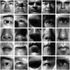
Figure 2: (a) Sample images form MNIST dataset, (b) and their corresponding samples from the second modality, drawn from USPS datasets. (c) Sample images from faces and face components from Extended Yale-B dataset; modalities are showed in different rows.

	Digits			Extended Yale-B
	ACC	NMI	ARI	ACC	NMI	ARI
CMVFC	47.6	73.56	38.12	66.84	72.03	40
TM-MSC	80.65	83.44	75.67	63.12	67.06	38.37
MSSC	81.65	85.33	77.36	80.3	82.78	50.18
MLRR	80.6	84.13	76.53	67.62	73.36	40.85
KMSSC	84.4	89.45	79.61	87.65	81.5	63.83
KMLRR	86.85	80.34	82.76	82.45	85.43	59.71
DMSC	95.15	92.09	90.22	99.22	98.89	98.38
VPCCA	98.78	96.72	97.35	99.71	99.52	99.19

Figure 3: Performance for different multi-modal clustering algorithms on two-modal handwritten digits made from MNIST and USPS and multi-modal facial components extracted from Yale-B dataset. Performance measures are clustering accuracy rate (ACC), normalized mutual information (NMI) and adjusted Rand index (ARI), all measures are in percent and the higher means the better. Here, we assume all modalities are available at the test time so VPCCA uses ${\bm{\mu}}_{0}$ of equation (8) is used. The results of variational PCCA method are averaged over 3 rials. The baseline subspace clustering methods are TM-MSC (Zhang et al., 2015), CMVFC (Cao et al., 2015), MSSC, MLRR , KMSSC, KMLRR (Abavisani and Patel, 2018b) and DMSC (Abavisani and Patel, 2018a) The results of the baseline methods are from (Abavisani and Patel, 2018a).

Handwritten Digits: We chose two famous handwritten digits datasets MNIST (Y. LeCun, 1998) and USPS (Hull, 1994) that consist of grayscale digit images of size $28\times 28$ pixels and $16\times 16$ pixels, respectively. To make multi-modal dataset, each digit image in the MNIST dataset is paired with an arbitrary sample of the same digit identity but from USPS dataset. This process guarantees that the images of both modalities are just sharing the same identity (label) of the digit but not the style of the handwriting. The handwritten digits datasets are used for single-modal training and also for multi-modal, with $M=2$, subspace clustering.

Multi-modal Facial Components: We also evaluate the proposed method on the multi-modal facial dataset used in (Abavisani and Patel, 2018a), where the Extended Yale-B dataset (Lee et al., 2005) was used as the base and 4 facial components are extracted, by cropping eyes, nose and mouth, and formed 5 different modalities, including the whole face image. All modalities are resized to images of size $28\times 28$ pixels. This dataset is composed of 64 frontal images of 38 individuals under different illuminations and is a standard dataset in subspace clustering studies. For this multi-modal data, we train the general deep probabilistic multi-view model that extends the deep probabilistic CCA to arbitrary number of views (4) (Appendix B).

Experimental design:

To make a fair comparison, in this set of experiments, the encoders and decoders are built of neural networks with similar architectures as those used in (Abavisani and Patel, 2018a), except that our model does not require the self-expressive layer, a linear fully connected layer with parameter matrix of size $N\times N$ coefficients. This key advantages of the proposed model, indeed, significantly reduces the total number of parameters specially for large input sizes.

Accordingly, the encoders (inference networks) of all modalities are composed of convolutional NN (CNN) layers while the decoders (observation networks) are built of transposed convolution layers. ReLU gate is used as nonlinearity for all the hidden units of the deep networks. The encoders specify $({\bm{\mu}}_{m},\text{diag}({\sigma}_{m}{i}^{2}))=f_{m}({\mathbf{x}}_{m};\theta_{m})$, where the variances are model by softplus function. An extra encoder network models the canonical correlations, $\text{diag}(p_{i})$, using the sigmoid function as the output gate. The observation likelihood functions of all the views, $p_{\theta_{m}}({\mathbf{x}}_{m}|{\mathbf{z}}_{m})$, are modeled by independent Bernoulli distributions with the mean parameter being specified by decoder networks, $g_{m}({\mathbf{z}}_{m};\theta_{m})$; the sigmoid functions are applied to estimate valid means of the distributions. To train the parameters of deep generative model, we used ADAM optimization (Kingma and Ba, 2014) with learning rate of $.0002$ and default hyper-parameters and minibatch size of 200 data points. Details of model architecture and experimental setup together with more empirical results are presented in appendix E.

Clustering is performed on the shared latent factor $\bm{\phi}$ using spectral clustering algorithm (Von Luxburg, 2007) on the k-nearest-neighbor graph, with number of neighbors $k=5$. As the last step, the spectral clustering discretizes the real-valued representation in the embedding space to extract the final partitioning. Clustering performance are measured using clustering Accuracy rate (ACC), Normalized Mutual Information (NMI) (Cai et al., 2005) and Adjusted Rand Index (ARI) (Rand, 1971) as performance metrics.

The clustering performance of the proposed method is compared against the well established subspace clustering methods TM-MSC (Zhang et al., 2015), CMVFC (Cao et al., 2015), MSSC, MLRR , KMSSC, KMLRR (Abavisani and Patel, 2018b) and DMSC (Abavisani and Patel, 2018a) that are used as the baselines methods for multi-modal setting. The results summarized in Table 3 show that the proposed deep generative model sets new state-of-the-art which, subsequently, highlights that the proposed method can efficiently leverage the extra modalities and extract the common underlying information among the modalities, that is the cluster memberships.

4 Conclusion

In this work, we developed a simple, yet powerful, tool for multi-view learning based on the probabilistic interpretation of CCA. A deep generative probabilistic model for multi-view data was studied. It has been shown that following the theoretical formulation of the linear probabilistic CCA model in conjunction with variational inference principles for deep generative networks, we can obtain a scalable end-to-end learning algorithm for multi-view data. Experimental results have shown that this can efficiently integrates the relationship between multiple views to obtain a more powerful representation which achieved state-of-the-arts performance on several downstream tasks. These indeed suggest that the proposed method is a proper way of extending variational inference to deep probabilistic multi-view learning.

Appendix A Proof of theorem 1

The marginal mean and covariance matrix of the joint views ${\mathbf{z}}=({\mathbf{z}}_{1},{\mathbf{z}}_{2})$ under the linear probabilistic model (2) are ${\bm{\mu}}=\begin{pmatrix}{\bm{W}}_{1}{\bm{\mu}}_{0}+{\bm{\mu}}_{{\epsilon}_{1}}\\ {\bm{W}}_{2}{\bm{\mu}}_{0}+{\bm{\mu}}_{{\epsilon}_{2}}\end{pmatrix}$ and ${\bm{\Sigma}}={\bm{W}}{\bm{W}}^{\top}+{\bm{\Psi}}$ where we define ${\bm{W}}=\begin{pmatrix}{\bm{W}}_{1}\\ {\bm{W}}_{2}\end{pmatrix}$ and ${\bm{\Psi}}=\begin{pmatrix}{\bm{\Psi}}_{1}&\mathbf{\bm{0}}\\ \mathbf{\bm{0}}&{\bm{\Psi}}_{2}\end{pmatrix}$, therefore, similar to the proof in [Bach and Jordan, 2005], the negative log-likelihood of the data can be written as

$$\ell_{1} =\frac{n(d_{1}+d_{2})}{2}\log 2\pi+\frac{n}{2}\log|{\bm{\Sigma}}|$$

$$\quad\quad+\frac{1}{2}\sum_{j=1}^{n}\mathop{\mathrm{tr}}{\bm{\Sigma}}^{{\scriptscriptstyle-1}}({\mathbf{z}}_{j}-{\bm{\mu}})({\mathbf{z}}_{j}-{\bm{\mu}})^{\top}$$

$$=\frac{n(d_{1}+d_{2})}{2}\log 2\pi+\frac{n}{2}\log|{\bm{\Sigma}}|$$

$$\quad\quad+\frac{n}{2}\mathop{\mathrm{tr}}{\bm{\Sigma}}^{{\scriptscriptstyle-1}}\tilde{{\bm{\Sigma}}}+\frac{n}{2}(\tilde{{\bm{\mu}}}-{\bm{\mu}}){\bm{\Sigma}}^{{\scriptscriptstyle-1}}(\tilde{{\bm{\mu}}}-{\bm{\mu}})^{\top}$$

Maximizing $\ell_{1}$ with respect to ${\bm{\mu}}$ results in a maximum ${\bm{\mu}}=\begin{pmatrix}{\bm{W}}_{1}{\bm{\mu}}_{0}+{\bm{\mu}}_{{\epsilon}_{1}}\\ {\bm{W}}_{2}{\bm{\mu}}_{0}+{\bm{\mu}}_{{\epsilon}_{2}}\end{pmatrix}=\begin{pmatrix}{\bm{\mu}}_{1}\\ {\bm{\mu}}_{2}\end{pmatrix}$ and the negative log-likelihood is reduced to

$$\ell_{1} =\frac{n(d_{1}+d_{2})}{2}\log 2\pi+\frac{n}{2}\log|{\bm{\Sigma}}|+\frac{n}{2}\mathop{\mathrm{tr}}{\bm{\Sigma}}^{{\scriptscriptstyle-1}}\tilde{{\bm{\Sigma}}}$$

The rest of the proof follows immediately along the line of proof in [Bach and Jordan, 2005].

Appendix B Generalization of probabilistic CCA

As an extension for probabilistic CCA to arbitrary number of views, [Archambeau and Bach, 2009] proposed a general probabilistic model as follows:

$${\mathbf{z}}_{m}= {\bm{W}}_{m}\bm{\phi}_{0}+{\bm{V}}_{m}\bm{\phi}_{m}+{\bm{\mu}}_{m}+\nu_{m},\forall m\in\{1,...,M\}$$ (10)

$$\quad{\bm{W}}_{m}\in\mathbb{R}^{d_{m}\times d_{0}},{\bm{V}}_{m}\in\mathbb{R}^{d_{m}\times q_{m}},$$

This model can also be viewed as multibattery factor analysis (MBFA) [Klami et al., 2014], [Browne, 1980] which describes the dependency between all the views by a single latent vector, $\bm{\phi}_{0}$, and explains away the view-specific variations by factors private to each view. Moreover, limiting to single view, this model also includes the probabilistic factor analysis and probabilistic PCA as a special cases if the view-specific dimensions are independent and isotropic [Archambeau and Bach, 2009].

Explaining the view-specific variations by the variance matrices for each view, we can represent the probabilistic multi-view model as

$$\bm{\phi} \sim\mathcal{N}({\bm{\mu}}_{0},\mathbf{I}_{d_{0}}),$$

$${\mathbf{z}}_{m}|\bm{\phi} \sim\mathcal{N}({\bm{W}}_{m}\bm{\phi}+{\bm{\mu}}_{{\epsilon}_{m}},{\bm{\Psi}}_{m}),$$ (11)

$$\quad{\bm{W}}_{m} \in\mathbb{R}^{d_{m}\times d_{0}},{\bm{\Psi}}_{m}\succcurlyeq 0,~{}m\in\{1,...,M\}$$

Where the latent factor $\bm{\phi}$ captures the common variations between all the views hence describing the essence of multi-view data. On the other hand, since the cluster memberships can be considered as a common information in all the views, this shared underlying representation is well suited for subspace clustering in multi-view setting. Let $({\bm{\mu}}_{m},{\bm{\Sigma}}_{mm})$ be the mean and covariance matrices of ${\mathbf{z}}_{m}$. Inspired by the maximum likelihood solutions of probabilistic CCA in theorem 1 and [Bach and Jordan, 2005], that reformulate the parameter estimate for the probabilistic model based on the classical CCA solutions, we can propose the following system of equation for the parameters of the probabilistic multi-view model

$${{\bm{W}}}_{m} ={\bm{\Sigma}}_{mm}^{1/2}{\bm{U}}_{m}{\bm{P}}_{d_{0}}^{1/2}{\bm{R}}$$

$${{\bm{\Psi}}}_{m} ={\bm{\Sigma}}_{mm}-{{\bm{W}}}_{m}{{\bm{W}}}_{m}^{\top}$$

$${{\bm{\mu}}}_{{\epsilon}_{m}} ={\bm{\mu}}_{m}-{{\bm{W}}}_{m}{\bm{\mu}}_{0}$$ (12)

Where ${\bm{P}}_{d_{0}}=\text{diag}([p_{0},...,p_{d_{0}}])$ with diagonal entries $p_{j}\in[0.,1.]$ and ${\bm{U}}_{m}$ are composed of orthonormal vectors $\{{\bm{u}}_{mi}\}$. To simplify the model, we assume ${\bm{U}}_{m}={\bm{U}},\forall m\in\{1,...,M\}$. The equations in (B) reduces to maximum likelihood estimate of PCCA for $m=2$ views, hence can be viewed as an extension of PCCA for multi-view with more than two views. Defining the correlation matrix as ${\bm{C}}_{lm}:={\bm{\Sigma}}_{ll}^{-1/2}{\bm{\Sigma}}_{lm}{\bm{\Sigma}}_{mm}^{-1/2}$ , equations in (B) imply that ${\bm{P}}_{d_{0}}$ and ${\bm{U}}$ are formed by the singular value and singular vectors of the correlation matrix, respectively, i.e. ${\bm{C}}_{lm}={\bm{U}}{\bm{P}}_{d_{0}}{\bm{U}}^{\top}$, therefore, analogous to the ML solution of PCCA, ${\bm{P}}_{d_{0}}$ and ${\bm{\Sigma}}_{mm}^{-1/2}{\bm{U}}_{m}$ can be interpreted as matrices of canonical correlations and canonical directions. This also implies that all the pairs of the views have similar correlation matrix.

In section 2.2, a closed form solution to infer $\{{\bm{\mu}}_{0},{\bm{\mu}}_{{\epsilon}_{m}}\}_{m=1}^{M}$ based on other variational statistics of the model is presented. We will also provide a simple treatments for ${\bm{U}}$ and ${\bm{R}}$. As a consequence, given the first and second order moments of the views together with the diagonal matrix of canonical correlations ${\bm{P}}_{d_{0}}$, one can infer the rest of the parameters for the multi-view generative model in (B). This, in fact, simplifies the variational inference network to just learn a compact set of parameters.

It is worth noting that, although the parametrization of model is based on a single shared latent factor (and also a single correlation matrix to explain the relationship between all the views) but it can be seen that the contribution of the shared factor in $m^{th}$ view is controlled by the factor loading ${\bm{W}}_{m}$ that is, in turn, a function of ${\bm{P}}_{d_{0}}$ and ${\bm{\Sigma}}_{mm}$, which is a view specific parameter. Therefore, the shared factor does not equally influence the views but instead its effect on each view varies by the strength of its projection ${\bm{W}}_{m}\bm{\phi}$ which results in dissimilar cross-covariances for the different pairs of views, ${\bm{\Sigma}}_{ml},m\neq l$ therefore offering flexibility to model uneven dependencies between the views.

Appendix C Some proofs of section 2.2

C.1 Proof of additive property of KL (2.2)

Conditional independence of the latent variables $\{{\mathbf{z}}_{m}|\bm{\phi}\}$ induced by the probabilistic graphical model of latent linear layer (2) implies that the approximate posterior of the set of latent variables can be factorized as

$$q_{\eta}({\mathbf{z}}|{\mathbf{x}})=q_{\eta}(\bm{\phi}|{\mathbf{x}})\prod_{m=1}^{M}q_{\eta}({\mathbf{z}}_{m}|\bm{\phi},{\mathbf{x}}).$$ (13)

In addition, assuming independent prior distribution on the latent variables, i.e. $p({\mathbf{z}})=p(\bm{\phi})\prod_{m=1}^{M}p({\mathbf{z}}_{m})$ leads to

$$D_{\mathrm{KL}}[q_{\eta}({\mathbf{z}}|{\mathbf{x}})\|p({\mathbf{z}})]=\int q_{\eta}(\bm{\phi}|{\mathbf{x}})\prod_{m=1}^{M}q_{\eta}({\mathbf{z}}_{m}|\bm{\phi},{\mathbf{x}})\times$$

$$\quad\quad\quad\log\frac{q_{\eta}(\bm{\phi}|{\mathbf{x}})\prod_{m=1}^{M}q_{\eta}({\mathbf{z}}_{m}|\bm{\phi},{\mathbf{x}})}{p(\bm{\phi})\prod_{m=1}^{M}p({\mathbf{z}}_{m})}$$

$$\quad\quad\quad=\int q_{\eta}(\bm{\phi}|{\mathbf{x}})\log\frac{q_{\eta}(\bm{\phi}|{\mathbf{x}})}{p(\bm{\phi})}$$

$$\quad\quad\quad+\sum_{m=1}^{M}\int q_{\eta}({\mathbf{z}}_{m}|\bm{\phi},{\mathbf{x}})\log\frac{q_{\eta}({\mathbf{z}}_{m}|\bm{\phi},{\mathbf{x}})}{p({\mathbf{z}}_{m})}$$

$$=D_{\mathrm{KL}}[q_{\eta}(\bm{\phi}|{\mathbf{x}})\|p(\bm{\phi})]+\sum_{m=1}^{M}D_{\mathrm{KL}}[q_{\eta}({\bm{\epsilon}}_{m}|{\mathbf{x}})\|p({\bm{\epsilon}}_{m})]\hfill\blacksquare$$

C.2 Proof of Lemma 1

Assuming isotropic multivariate Gaussian priors on the latent variables as $\bm{\phi}\sim\mathcal{N}(\mathbf{0},\lambda_{0}^{-1}\mathbf{I})$, ${\bm{\epsilon}}_{m}\sim\mathcal{N}(\mathbf{0},\lambda_{m}^{-1}\mathbf{I})$ and specifying the approximate posteriors as Gaussian distributed vectors with diagonal covariances results in closed form solutions for the KL divergence terms [Kingma and Welling, 2013] as

$$D_{\mathrm{KL}}[q_{\eta}(\bm{\phi}|{\mathbf{x}})\|p(\bm{\phi})] =\frac{1}{2}\lambda_{0}\|{\bm{\mu}}_{0}\|^{2}+$$

$$\frac{1}{2}\sum_{i=1}^{d_{0}}(\lambda_{0}-\log\lambda_{0}-1)$$

$$D_{\mathrm{KL}}[q_{\eta}({\bm{\epsilon}}_{m}|{\mathbf{x}})\|p({\bm{\epsilon}}_{m})] =\frac{1}{2}\lambda_{m}\|{\bm{\mu}}_{{\epsilon}_{m}}\|^{2}+$$

$$\frac{1}{2}\sum_{i=1}^{d_{m}}(\lambda_{m}{\sigma}_{mi}^{2}-\log\lambda_{m}{\sigma}_{mi}^{2}-1)$$

Splitting the terms in the KL divergence to those depending on the mean variables and the remaining ones results

$$\min_{{\bm{\mu}}_{0}} \frac{1}{2}\lambda_{0}\|{\bm{\mu}}_{0}\|^{2}+\frac{1}{2}\sum_{m=1}^{M}\lambda_{m}\|{\bm{\mu}}_{{\epsilon}_{m}}\|^{2}+\mathcal{K}$$

$$\text{s.t. }{\bm{\mu}}_{{\epsilon}_{m}} ={\bm{\mu}}_{m}-{\bm{W}}_{m}{\bm{\mu}}_{0},\quad\forall m\in\{1,...,M\}$$

Now, solving this constraint optimization problem using the method of Lagrange multipliers leads to the optimal minimizer

$${\bm{\mu}}_{0}^{*}=(\lambda_{0}\mathbf{I}+\sum_{m=1}^{M}\lambda_{m}{\bm{W}}_{m}^{\top}{\bm{W}}_{m})^{-1}(\sum_{m=1}^{M}\lambda_{m}{\bm{W}}_{m}^{\top}{\bm{\mu}}_{m}).$$

This provides an analytical approach to optimally recover ${\bm{\mu}}_{0}$ from the parameters of the model.

Appendix D 2-D embedding

Figures 4 depict the 2D t-SNE embeddings of the shared latent representations for multi-view and multi-modal setting, respectively. They verify that the representation of the images of different classes are well separated in the shared latent space.

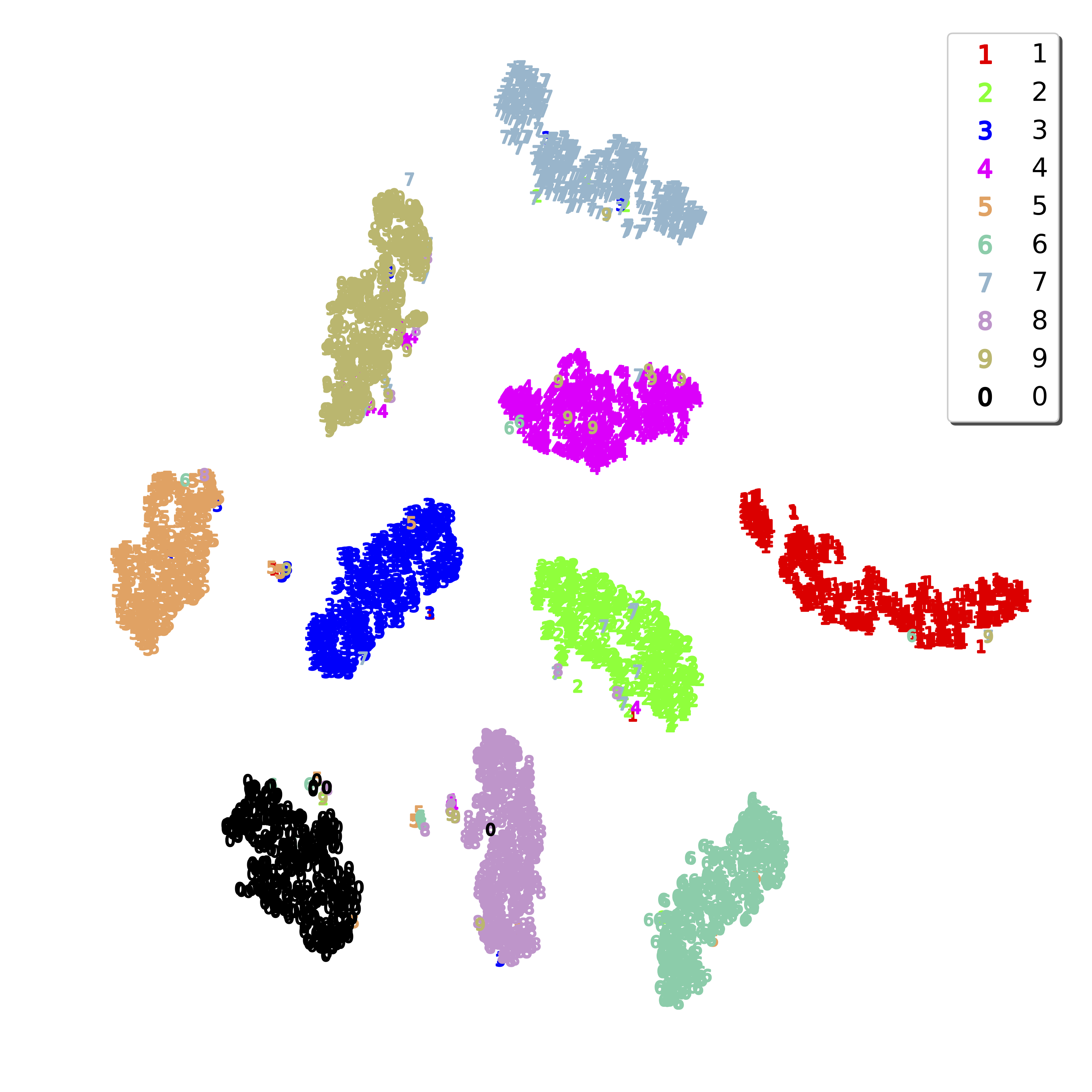
Figure 4: 2D t-SNE embedding of the mean of shared representation ${\bm{\mu}}_{0}$.

Appendix E Model architecture and training procedure

E.1 Two-view noisy MNIST experiments

The parameters of each algorithm are tuned through cross validation with grid search over $p_{dropout}\in\{.0,.2\}$ the variance of the shared representation $\bm{\phi}$ $\lambda_{0}^{{\scriptscriptstyle-1}}\in\{100.,500.,2000.,5000.\}$ and equal variance for residual errors ${\bm{\epsilon}}_{1},{\bm{\epsilon}}_{2}$ in range $\lambda_{0}^{{\scriptscriptstyle-1}}\in\{8.,4.,2.,1.,.5,.25,.125\}$. Results are averaged over 3 trails.

The dimensionality of the shared representation was $d_{0}=30$ and the dimensionality of the latent factors were $d_{1}=d_{2}=60$.

Weight decay of 0.0001 was applied as the regularization for all the parameters of NNs.

E.2 Multi-modal clustering experiments

digits: The dimensionality of the shared representation was $d_{0}=30$ and the dimensionality of the latent factors were $d_{1}=d_{2}=60$.

The parameters of each algorithm are tuned through cross validation with grid search over $p_{dropout}\in\{.0,.2\}$ the variance of the shared representation $\bm{\phi}$ $\lambda_{0}^{{\scriptscriptstyle-1}}\in\{1.,5.,20.,100.,500.,2000.\}$ and equal variance for residual errors ${\bm{\epsilon}}_{1},{\bm{\epsilon}}_{2}$ in range $\lambda_{0}^{{\scriptscriptstyle-1}}\in\{8.,4.,2.,1.,.5,.25,.125\}$.

Yale-B facial components: The dimensionality of the shared representation was $d_{0}=120$ and the dimensionality of the latent factors were $d_{1}=d_{2}=160$.

The parameters of each algorithm are tuned through cross validation with grid search over $p_{dropout}\in\{.0,.2\}$ the variance of the shared representation $\bm{\phi}$ $\lambda_{0}^{{\scriptscriptstyle-1}}\in\{.2,1.,5.,20.,100.,500.,2000.\}$ and equal variance for residual errors ${\bm{\epsilon}}_{1},{\bm{\epsilon}}_{2}$ in range $\lambda_{0}^{{\scriptscriptstyle-1}}\in\{8.,4.,2.,1.,.5,.25,.125\}$.

In both experiments a weight decay of 0.0001 was applied as the regularization for all the parameters of NNs.

References

- Abavisani and Patel (2018a) Mahdi Abavisani and Vishal M Patel. Deep multimodal subspace clustering networks. IEEE Journal of Selected Topics in Signal Processing, 12(6):1601–1614, 2018a.
- Abavisani and Patel (2018b) Mahdi Abavisani and Vishal M Patel. Multimodal sparse and low-rank subspace clustering. Information Fusion, 39:168–177, 2018b.
- Andrew et al. (2013) Galen Andrew, Raman Arora, Jeff Bilmes, and Karen Livescu. Deep canonical correlation analysis. In International Conference on Machine Learning, pages 1247–1255, 2013.
- Archambeau and Bach (2009) Cédric Archambeau and Francis R Bach. Sparse probabilistic projections. In Advances in neural information processing systems, pages 73–80, 2009.
- Bach and Jordan (2003) Francis R. Bach and Michael I. Jordan. Kernel independent component analysis. J. Mach. Learn. Res., 3:1–48, March 2003. ISSN 1532-4435.
- Bach and Jordan (2005) Francis R Bach and Michael I Jordan. A probabilistic interpretation of canonical correlation analysis. Technical Report 688, Department of Statistics, University of California, Berkeley, 2005.
- Browne (1979) Michael W Browne. The maximum-likelihood solution in inter-battery factor analysis. British Journal of Mathematical and Statistical Psychology, 32(1):75–86, 1979.
- Browne (1980) Michael W Browne. Factor analysis of multiple batteries by maximum likelihood. British Journal of Mathematical and Statistical Psychology, 33(2):184–199, 1980.
- Cai et al. (2005) Deng Cai, Xiaofei He, and Jiawei Han. Document clustering using locality preserving indexing. IEEE Transactions on Knowledge and Data Engineering, 17(12):1624–1637, 2005.
- Cao et al. (2015) Xiaochun Cao, Changqing Zhang, Chengju Zhou, Huazhu Fu, and Hassan Foroosh. Constrained multi-view video face clustering. IEEE Transactions on Image Processing, 24(11):4381–4393, 2015.
- Chaudhuri et al. (2009) Kamalika Chaudhuri, Sham M Kakade, Karen Livescu, and Karthik Sridharan. Multi-view clustering via canonical correlation analysis. In Proceedings of the 26th annual international conference on machine learning, pages 129–136. ACM, 2009.
- Damianou et al. (2012) Andreas Damianou, Carl Ek, Michalis Titsias, and Neil Lawrence. Manifold relevance determination. arXiv preprint arXiv:1206.4610, 2012.
- Hardoon et al. (2004) David R. Hardoon, Sandor R. Szedmak, and John R. Shawe-taylor. Canonical correlation analysis: An overview with application to learning methods. Neural Comput., 16(12):2639–2664, December 2004. ISSN 0899-7667.
- Hotelling (1992) Harold Hotelling. Relations between two sets of variates. In Breakthroughs in statistics, pages 162–190. Springer, 1992.
- Hull (1994) Jonathan J. Hull. A database for handwritten text recognition research. IEEE Transactions on pattern analysis and machine intelligence, 16(5):550–554, 1994.
- Ji et al. (2017) Pan Ji, Tong Zhang, Hongdong Li, Mathieu Salzmann, and Ian Reid. Deep subspace clustering networks. In Advances in Neural Information Processing Systems, pages 24–33, 2017.
- Jordan et al. (1999) Michael I Jordan, Zoubin Ghahramani, Tommi S Jaakkola, and Lawrence K Saul. An introduction to variational methods for graphical models. Machine learning, 37(2):183–233, 1999.
- Karami et al. (2019) Mahdi Karami, Dale Schuurmans, Jascha Sohl-Dickstein, Laurent Dinh, and Daniel Duckworth. Invertible convolutional flow. In Advances in Neural Information Processing Systems, pages 5636–5646, 2019.
- Kingma and Ba (2014) Diederik P Kingma and Jimmy Ba. Adam: A method for stochastic optimization. arXiv preprint arXiv:1412.6980, 2014.
- Kingma and Welling (2013) Diederik P Kingma and Max Welling. Auto-encoding variational bayes. arXiv preprint arXiv:1312.6114, 2013.
- Kingma et al. (2019) Diederik P Kingma, Max Welling, et al. An introduction to variational autoencoders. Foundations and Trends® in Machine Learning, 12(4):307–392, 2019.
- Klami and Kaski (2007) Arto Klami and Samuel Kaski. Local dependent components. In Proceedings of the 24th international conference on Machine learning, pages 425–432. ACM, 2007.
- Klami et al. (2013) Arto Klami, Seppo Virtanen, and Samuel Kaski. Bayesian canonical correlation analysis. Journal of Machine Learning Research, 14(Apr):965–1003, 2013.
- Klami et al. (2014) Arto Klami, Seppo Virtanen, Eemeli Leppäaho, and Samuel Kaski. Group factor analysis. IEEE transactions on neural networks and learning systems, 26(9):2136–2147, 2014.
- Lee et al. (2005) Kuang-Chih Lee, Jeffrey Ho, and David J Kriegman. Acquiring linear subspaces for face recognition under variable lighting. IEEE Transactions on Pattern Analysis & Machine Intelligence, (5):684–698, 2005.
- Lopez-Paz et al. (2014) David Lopez-Paz, Suvrit Sra, Alex Smola, Zoubin Ghahramani, and Bernhard Schölkopf. Randomized nonlinear component analysis. In International Conference on Machine Learning, pages 1359–1367, 2014.
- Ngiam et al. (2011) Jiquan Ngiam, Aditya Khosla, Mingyu Kim, Juhan Nam, Honglak Lee, and Andrew Y Ng. Multimodal deep learning. In Proceedings of the 28th international conference on machine learning (ICML-11), pages 689–696, 2011.
- Rand (1971) William M Rand. Objective criteria for the evaluation of clustering methods. Journal of the American Statistical association, 66(336):846–850, 1971.
- Rezende and Mohamed (2015) Danilo Rezende and Shakir Mohamed. Variational inference with normalizing flows. In Proceedings of The 32nd International Conference on Machine Learning, pages 1530–1538, 2015.
- Rezende et al. (2014) Danilo Jimenez Rezende, Shakir Mohamed, and Daan Wierstra. Stochastic backpropagation and approximate inference in deep generative models. arXiv preprint arXiv:1401.4082, 2014.
- Shon et al. (2006) Aaron Shon, Keith Grochow, Aaron Hertzmann, and Rajesh PN Rao. Learning shared latent structure for image synthesis and robotic imitation. In Advances in neural information processing systems, pages 1233–1240, 2006.
- Srivastava et al. (2014) Nitish Srivastava, Geoffrey Hinton, Alex Krizhevsky, Ilya Sutskever, and Ruslan Salakhutdinov. Dropout: a simple way to prevent neural networks from overfitting. The journal of machine learning research, 15(1):1929–1958, 2014.
- Tang et al. (2017) Qingming Tang, Weiran Wang, and Karen Livescu. Acoustic feature learning via deep variational canonical correlation analysis. arXiv preprint arXiv:1708.04673, 2017.
- Von Luxburg (2007) Ulrike Von Luxburg. A tutorial on spectral clustering. Statistics and computing, 17(4):395–416, 2007.
- Wang et al. (2015) Weiran Wang, Karen Livescu, and Jeff Bilmes. On Deep Multi-View Representation Learning. Icml, 37, 2015.
- Wang et al. (2016) Weiran Wang, Xinchen Yan, Honglak Lee, and Karen Livescu. Deep variational canonical correlation analysis. arXiv preprint arXiv:1610.03454, 2016.
- Williams and Seeger (2001) Christopher KI Williams and Matthias Seeger. Using the nyström method to speed up kernel machines. In Advances in neural information processing systems, pages 682–688, 2001.
- Xia et al. (2014) Rongkai Xia, Yan Pan, Lei Du, and Jian Yin. Robust multi-view spectral clustering via low-rank and sparse decomposition. In Twenty-Eighth AAAI Conference on Artificial Intelligence, 2014.
- Y. LeCun (1998) C. Cortes Y. LeCun. The mnist database of handwritten digit. 1998.
- Zhang et al. (2015) Changqing Zhang, Huazhu Fu, Si Liu, Guangcan Liu, and Xiaochun Cao. Low-rank tensor constrained multiview subspace clustering. In Proceedings of the IEEE international conference on computer vision, pages 1582–1590, 2015.