ADJACENCY LABELLING FOR PLANAR GRAPHS (AND BEYOND)

We show that there exists an adjacency labelling scheme for planar graphs where each vertex of an $n$-vertex planar graph $G$ is assigned a $(1+o(1))\log_{2}n$-bit label and the labels of two vertices $u$ and $v$ are sufficient to determine if $uv$ is an edge of $G$. This is optimal up to the lower order term and is the first such asymptotically optimal result. An alternative, but equivalent, interpretation of this result is that, for every positive integer $n$, there exists a graph $U_{n}$ with $n^{1+o(1)}$ vertices such that every $n$-vertex planar graph is an induced subgraph of $U_{n}$. These results generalize to a number of other graph classes, including bounded genus graphs, apex-minor-free graphs, bounded-degree graphs from minor closed families, and $k$-planar graphs.

1 Introduction

A family $\mathcal{G}$ of graphs has an $f(n)$-bit adjacency labelling scheme if there exists a function $A:(\{0,1\}^{*})^{2}\to\{0,1\}$ such that for every $n$-vertex graph $G\in\mathcal{G}$ there exists $\ell:V(G)\to\{0,1\}^{*}$ such that $|\ell(v)|\le f(n)$ for each vertex $v$ of $G$ and such that, for every two vertices $v,w$ of $G$,

$$A(\ell(v),\ell(w))=\cases{0}&\text{ifvw\not\in E(G);}\\ 1\text{ifvw\in E(G).}$$

Let $\log x:=\log_{2}x$ denote the binary logarithm of $x$. In this paper we prove the following result:

Theorem 1.

The family of planar graphs has a $(1+o(1))\log n$-bit adjacency labelling scheme.

Theorem 1 is optimal up to the lower order $o(\log n)$ term, which is $\mathcal{O}\left(\sqrt{\log n\log\log n}\right)$ in our proof. An alternative, but equivalent, interpretation of Theorem 1 is that, for every integer $n\ge 1$, there exists a graph $U_{n}$ with $n^{1+o(1)}$ vertices such that every $n$-vertex planar graph is isomorphic to some vertex-induced subgraph of $U_{n}$.

Note that the proof of Theorem 1 is constructive: it gives an algorithm producing the labels in $\mathcal{O}(n\log n)$ time.

1.1 Previous Work

The current paper is the latest in a series of results dating back to Kannan, Naor, and Rudich [kannan.naor.ea:implicit0, kannan.naor.ea:implicit] and Muller [muller:local] who defined adjacency labelling schemes and described $\mathcal{O}(\log n)$-bit adjacency labelling schemes for several classes of graphs, including planar graphs. Since this initial work, adjacency labelling schemes and, more generally, informative labelling schemes have remained a very active area of research [adjiashvili.rotbart:labeling, alstrup.kaplan.ea:adjacency, abrahamsen.alstrup.ea:near-optimal, alstrup.dahlgaard.ea:sublinear, alstrup.gortz.ea:distance, alstrup.gavoille.ea:simpler, alstrup.rauhe:improved, Alon17].

Here we review results most relevant to the current work, namely results on planar graphs and their supporting results on trees and bounded-treewidth graphs. First, a superficial review: Planar graphs have been shown to have $(c+o(1))\log n$-bit adjacency labelling schemes for successive values of $c=6,4,3,2,\tfrac{4}{3}$ and finally Theorem 1 gives the optimal result $c=1$. We now give details of these results.

Muller’s scheme for planar graphs [muller:local] is based on the fact that planar graphs are 5-degenerate. This scheme orients the edges of the graph so that each vertex has 5 outgoing edges, assigns each vertex $v$ an arbitrary $\lceil\log n\rceil$-bit identifier, and assigns a label to $v$ consisting of $v$’s identifier and the identifiers of the targets of $v$’s outgoing edges. In this way, each vertex $v$ is assigned a label of length at most $6\lceil\log n\rceil$. Kannan, Naor, and Rudich [kannan.naor.ea:implicit] use a similar approach that makes use of the fact that planar graphs have arboricity 3 (so their edges can be partitioned into three forests [nash-williams:edge-disjoint]) to devise an adjacency labelling scheme for planar graphs whose labels have length at most $4\lceil\log n\rceil$.

A number of $(1+o(1))\log n$-bit adjacency labelling schemes for forests have been devised [chung:universal, alstrup.rauhe:improved, alstrup.dahlgaard.ea:optimal], culminating with a recent $(\log n+\mathcal{O}(1))$-bit adjacency labelling scheme [alstrup.dahlgaard.ea:optimal] for forests. Combined with the fact that planar graphs have arboricity 3, these schemes imply $(3+o(1))\log n$-bit adjacency labelling schemes for planar graphs.

A further improvement, also based on the idea of partitioning the edges of a planar graph into simpler graphs was obtained by Gavoille and Labourel [gavoille.labourel:shorter]. Generalizing the results for forests, they describe a $(1+o(1))\log n$-bit adjacency labelling scheme for $n$-vertex graphs of bounded treewidth. As is well known, the edges of a planar graph can be partitioned into two sets, each of which induces a bounded treewidth graph [goncalves.gabow.ea:edge]. This results in a $(2+o(1))\log n$-bit adjacency labelling scheme for planar graphs.

Very recently, Bonamy, Gavoille, and Pilipczuk [bonamy.gavoille.ea:shorter] described a $(4/3+o(1))\log n$-bit adjacency labelling scheme for planar graphs based on a recent graph product structure theorem of Dujmović et al. [dujmovic.joret.ea:planar]. This product structure theorem states that any planar graph is a subgraph of a strong product $H\boxtimes P$ where $H$ is a bounded-treewidth graph and $P$ is a path. See Figure 1. It is helpful to think of $H\boxtimes P$ as a graph whose vertices can be partitioned into $h:=|V(P)|$ rows $H_{1},\dots,H_{h}$, each of which induces a copy of $H$ and with vertical and diagonal edges joining corresponding and adjacent vertices between consecutive rows.

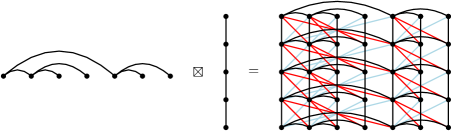
Figure 1: The strong product $H\boxtimes P$ of a tree $H$ and a path $P$.

The product structure theorem quickly leads to a $(1+o(1))\log(mh)$-bit labelling scheme where $m:=|V(H)|$ and $h:=|V(P)|$ by using a $(1+o(1))\log m$-bit labelling scheme for $H$ (a bounded treewidth graph), a ${\lceil\log{h}\rceil}$-bit labelling scheme for $P$ (a path), and a constant number of bits to locally encode the subgraph of $H\boxtimes P$ (of constant arboricity). However, for an $n$-vertex graph $G$ that is a subgraph of $H\boxtimes P$ in the worst case $m$ and $h$ are each $\Omega(n)$, so this offers no immediate improvement over the existing $(2+o(1))\log n$-bit scheme.

Bonamy, Gavoille, and Pilipczuk improve upon this by cutting $P$ (and hence $G$) into subpaths of length $n^{1/3}$ in such a way that this corresponds to removing $\mathcal{O}(n^{2/3})$ vertices of $G$ that have a neighbourhood of size $\mathcal{O}(n^{2/3})$. The resulting (cut) graph is a subgraph of $H^{\prime}\boxtimes P^{\prime}$ where $H^{\prime}$ has bounded treewidth, $|H^{\prime}|\le n$, and $P^{\prime}$ is a path of length $n^{1/3}$ so it has a labelling scheme in which each vertex has a label of length $(1+o(1))\log(|H^{\prime}|\cdot|P^{\prime}|)\le(4/3+o(1))\log n$. A slight modification of this scheme allows for the $\mathcal{O}(n^{2/3})$ boundary vertices adjacent to the cuts to have shorter labels, of length only $(2/3+o(1))\log n$. The cut vertices and the boundary vertices induce a bounded-treewidth graph of size $\mathcal{O}(n^{2/3})$. The vertices in this graph receive secondary labels of length $(2/3+o(1))\log n$. In this way, every vertex receives a label of length at most $(4/3+o(1))\log n$.

1.2 New Results

The adjacency labelling scheme described in the current paper is also based on the product structure theorem for planar graphs, but it avoids cutting the path $P$, and thus avoids boundary vertices that take part in two different labelling schemes. Instead, it uses a weighted labelling scheme on the rows $H_{1},\dots,H_{h}$ of $H\boxtimes P$ in which vertices that belong to $H_{i}$ receive a label of length $(1+o(1))\log n-\log W_{i}$ where $W_{i}$ is related to the number of vertices of $G$ contained in $H_{i}$ and $H_{i-1}$. The vertices of $G$ in row $i$ participate in a secondary labelling scheme for the subgraph of $G$ contained in $H_{i}$ and $H_{i-1}$ and the labels in this scheme have length $\log W_{i}+o(\log n)$. Thus every vertex receives two labels, one of length $(1+o(1))\log n-\log W_{i}$ and another of length $\log W_{i}+o(\log n)$ for a total label length of $(1+o(1))\log n$.

The key new technique that allows all of this to work is that the labelling schemes of the rows $H_{1},\dots,H_{h}$ are not independent. All of these labelling schemes are based on a single balanced binary search tree $T$ that undergoes insertions and deletions resulting in a sequence of related binary search trees $T_{1},\dots,T_{h}$ where each $T_{i}$ represents all vertices of $G$ in $H_{i}$ and $H_{i-1}$ and the label assigned to a vertex of $H_{i}$ is essentially based on a path from the root of $T_{i}$ to some vertex of $T_{i}$. By carefully maintaining the binary search tree $T$, the trees $T_{i-1}$ and $T_{i}$ are similar enough so that the label for $v$ in $H_{i}$ can be obtained, with $o(\log n)$ additional bits from the label for $v$ in $H_{i-1}$.

The product structure theorem has been generalized to a number of additional graph families including bounded-genus graphs, apex-minor free graphs, bounded-degree graphs from minor-closed families, $k$-planar graphs, powers of bounded-degree bounded genus graphs, and $k$-nearest neighbour graphs of points in $\mathbb{R}^{2}$ [dujmovic.joret.ea:planar, dujmovic.morin.ea:structure]. As a side-effect of designing a labelling scheme to work directly on subgraphs of a strong product $H\boxtimes P$, where $H$ has bounded treewidth and $P$ is a path, we obtain $(1+o(1))\log n$-bit labelling schemes for all of these graph families. All of these results are optimal up to the lower order term.

A graph is apex if it has a vertex whose removal leaves a planar graph. A graph is $k$-planar if it has a drawing in the plane in which each edge is involved in at most $k$ crossings. Such graphs provide a natural generalisation of planar graphs, and have been extensively studied [kobourov.liotta.ea:annotated]. The definition of $k$-planar graphs naturally generalises for other surfaces. A graph $G$ is $(g,k)$-planar if it has a drawing in some surface of Euler genus at most $g$ in which each edge of $G$ is involved in at most $k$ crossings. Note that already $1$-planar graphs are not minor closed. The generalization of Theorem 1 provided by known product structure theorems is summarized in the following result:

Theorem 2.

For every fixed integer $t\geq 1$, the family of all graphs $G$ such that $G$ is a subgraph of $H\boxtimes P$ for some graph $H$ of treewidth $t$ and some path $P$ has a $(1+o(1))\log n$-bit adjacency labelling scheme. This includes the following graph classes:

1. graphs of bounded genus and, more generally, apex-minor free graphs;

2. bounded degree graphs that exclude a fixed graph as a minor; and

3. $k$-planar graphs and, more generally, $(g,k)$-planar graphs.

The case of graphs of bounded degree from minor-closed classes (point 2 in Theorem 2) is particularly interesting since, prior to the current work, the best known bound for adjacency labelling schemes in planar graphs of bounded degree was the same as for general planar graphs, i.e., $(4/3+o(1))\log n$. On the other hand, our Theorem 2 now gives an asymptotically optimal bound of $(1+o(1))\log n$ for graphs of bounded degree from any proper minor-closed class.

1.3 Outline

The remainder of the paper is organized as follows. Section 2 reviews some preliminary definitions and easy results. Section 3 describes a new type of balanced binary search tree that has the specific properties needed for our application. Section LABEL:sec:pxp solves a special case, where $G$ is an $n$-vertex subgraph of $P_{1}\boxtimes P_{2}$ where $P_{1}$ and $P_{2}$ are both paths. We include it to highlight the generic idea behind our adjacency labelling scheme. Section LABEL:sec:hxp solves the general case in which $G$ is an $n$-vertex subgraph of $H\boxtimes P$ where $H$ has bounded treewidth and $P$ is a path. Section LABEL:sec:conclusion concludes with a discussion of the computational complexity of assigning labels and testing adjacency and presents directions for future work.

2 Preliminaries

All graphs we consider are finite and simple. The vertex and edge sets of a graph $G$ are denoted by $V(G)$ and $E(G)$, respectively. The size of a graph $G$ is denoted by $|G|:=|V(G)|$.

For any graph $G$ and any vertex $v\in V(G)$, let $N_{G}(v):=\{w\in V(G):vw\in E(G)\}$ and $N_{G}[v]:=N_{G}(v)\cup\{v\}$ denote the open neighbourhood and closed neighbourhood of $v$ in $G$, respectively.

2.1 Prefix-Free Codes

For a string $s=s_{1},\dots,s_{k}$, we use $|s|:=k$ to denote the length of $s$. A string $s_{1},\dots,s_{k}$ is a prefix of a string $t_{1},\dots,t_{\ell}$ if $k\le\ell$ and $s_{1},\dots,s_{k}=t_{1},\dots,t_{k}$. A prefix-free code $c:X\to\{0,1\}^{*}$ is a one-to-one function in which $c(x)$ is not a prefix of $c(y)$ for any two distinct $x,y\in X$. Let $\mathbb{N}$ denote the set of non-negative integers. The following is a classic observation of Elias from 1975.

Lemma 3 (Elias [elias:universal]).

There exists a prefix-free code $\gamma:\mathbb{N}\to\{0,1\}^{*}$ such that, for each $i\in\mathbb{N}$, $|\gamma(i)|\le 2\lfloor\log(i+1)\rfloor+1$.

In the remainder of the paper, $\gamma$ (which we call an Elias encoding) will be used extensively, without referring systematically to Lemma 3.

2.2 Labelling Schemes Based on Binary Trees

A binary tree $T$ is a rooted tree in which each node except the root is either the left or right child of its parent and each node has at most one left and at most one right child. For any node $x$ in $T$, $P_{T}(x)$ denotes the path from the root of $T$ to $x$. The length of a path $P$ is the number of edges in $P$, i.e., $|P|-1$. The depth, $d_{T}(x)$ of $x$ is the length of $P_{T}(x)$. The height of $T$ is $h(T):=\max_{x\in V(T)}d_{T}(x)$. A perfectly balanced binary tree is any binary tree $T$ of height $h(T)=\lfloor\log|T|\rfloor$, where $|T|:=|V(T)|$ denotes the number of nodes in $T$.

A binary tree is full if each non-leaf node has exactly two children. For a binary tree $T$, we let $T^{+}$ denote the full binary tree obtained by attaching to each node $x$ of $T$ $2-c_{x}$ leaves where $c_{x}\in\{0,1,2\}$ is the number of children of $x$. We call the leaves of $T^{+}$ the external nodes of $T$. (Note that none of these external nodes are in $T$ and, for any non-empty $T$, $h(T^{+})=h(T)+1$.)

A node $a$ in $T$ is a $T$-ancestor of a node $x$ in $T$ if $a\in V(P_{T}(x))$. If $a$ is a $T$-ancestor of $x$ then $x$ is a $T$-descendant of $a$. (Note that a node is a $T$-ancestor and $T$-descendant of itself.) For a subset of nodes $X\subseteq V(T)$, the lowest common $T$-ancestor of $X$ is the maximum-depth node $a\in V(T)$ such that $a$ is a $T$-ancestor of $x$ for each $x\in X$.

Let $P_{T}(x_{r})=x_{0},\dots,x_{r}$ be a path from the root $x_{0}$ of $T$ to some node $x_{r}$ (possibly $r=0$). Then the signature of $x_{r}$ in $T$, denoted $\sigma_{T}(x_{r})$ is a binary string $b_{1},\dots,b_{r}$ where $b_{i}=0$ if and only if $x_{i}$ is the left child of $x_{i-1}$. Note that the signature of the root of $T$ is the empty string.

A binary search tree $T$ is a binary tree whose node set $V(T)$ consists of distinct real numbers and that has the binary search tree property: For each node $x$ in $T$, $z<x$ for each node $z$ in $x$’s left subtree and $z>x$ for each node $z$ in $x$’s right subtree. For any $x\in\mathbb{R}\setminus V(T)$, the search path $P_{T}(x)$ in $T$ is the unique root-to-leaf path $v_{0},\dots,v_{r}$ in $T^{+}$ such that adding $x$ as a (left or right, as appropriate) child of $v_{r-1}$ in $T$ would result in a binary search tree $T^{\prime}$ with $V(T^{\prime})=V(T)\cup\{x\}$.

The following observation allows us to compare values in a binary search tree just given their signatures in the tree.

Observation 4.

For any binary search tree $T$ and any nodes $x$, $y$ in $T$, we have $x<y$ if and only if $\sigma_{T}(x)$ is lexicographically less than $\sigma_{T}(y)$.

Let $\mathbb{R}^{+}$ denote the set of positive real numbers. The following is a folklore result about biased binary search trees, but we sketch a proof here for completeness.

Lemma 5.

For any finite $S\subset\mathbb{R}$ and any function $w:S\to\mathbb{R}^{+}$, there exists a binary search tree $T$ with $V(T)=S$ such that, for each $y\in S$, $d_{T}(y)\le\log(W/w(y))$, where $W:=\sum_{y\in S}w(y)$.

Proof.

The proof is by induction on $|S|$. The base case $|S|=0$ is vacuously true. For any $x\in\mathbb{R}$, let $S_{<x}:=\{y\in S:y<x\}$ and $S_{>x}:=\{y\in S:y>x\}$. For $|S|\ge 1$, choose the root of $T$ to be the unique node $y_{0}\in S$ such that $\sum_{z\in S_{<y_{0}}}w(z)\le W/2$ and $\sum_{z\in S_{>y_{0}}}<W/2$. Apply induction on $S_{<y_{0}}$ and $S_{>y_{0}}$ to obtain the left and right subtrees of $T$, respectively.

Then $d_{T}(y_{0})=0=\log 1\le\log(W/w(y_{0}))$. For each $y\in S_{<y_{0}}$,

$$d_{T}(y)\le 1+\log\left(\frac{\sum_{z\in S_{<y_{0}}}w(z)}{w(y)}\right)\le 1+\log\left(\frac{W/2}{w(y)}\right)=\log\left(\frac{W}{w(y)}\right),$$

and the same argument shows that $d_{T}(y)<\log(W/w(y))$ for each $y\in S_{>y_{0}}$. ∎

The following fact about binary search trees is useful, for example, in the deletion algorithms for several types of balanced binary search trees [morin:open, Section 6.2.3], see Figure 2:

Figure 2: An illustration of Observation 6: (1) $\sigma_{T}(y_{1})=11000$ and $\sigma_{T}(x_{1})=1\mbox{\sout{1000}}$ (2) $\sigma_{T}(y_{2})=10\mbox{\sout{011}}$ and $\sigma_{T}(x_{2})=10011$.

Observation 6.

Let $T$ be a binary search tree and let $x$, $y$ be nodes in $T$ such that $x<y$ and there is no node $z$ in $T$ such that $x<z<y$, i.e., $x$ and $y$ are consecutive in the sorted order of $V(T)$. Then

1. (if $y$ has no left child) $\sigma_{T}(x)$ is obtained from $\sigma_{T}(y)$ by removing all trailing 0’s and the last 1; or

2. (if $y$ has a left child) $\sigma_{T}(x)$ is obtained from $\sigma_{T}(y)$ by appending a 0 followed by $d_{T}(y)-d_{T}(x)-1$ 1’s.

Therefore, there exists a function $D:(\{0,1\}^{*})^{2}\to\{0,1\}^{*}$ such that, for every binary search tree $T$ and for every two consecutive nodes $x,y$ in the sorted order of $V(T)$, there exists $\delta_{T}(y)\in\{0,1\}^{*}$ with $|\delta_{T}(y)|=\mathcal{O}(\log h(T))$ such that $D(\sigma_{T}(y),\delta_{T}(y))=\sigma_{T}(x)$.

The bitstring $\delta_{T}(y)$ from Observation 6 is obtained as follows: It consists of a first bit indicating whether $y$ has a left child in $T$ or not and, in case $y$ does have a left child, an Elias encoding $\gamma(s)$ of the value $s:=d_{T}(y)-d_{T}(x)-1$. More precisely, $\delta_{T}(y)=0$ or $\delta_{T}(y)=1,\gamma(s)$.

Putting some of the preceding results together we obtain the following useful coding result.

Lemma 7.

There exists a function $A:(\{0,1\}^{*})^{2}\to\{-1,0,1,\perp\}$ such that, for any $h\in\mathbb{N}$, and any $w:\{1,\dots,h\}\to\mathbb{R}^{+}$ there is a prefix-free code $\alpha:\{1,\dots,h\}\to\{0,1\}^{*}$ such that

1. for each $i\in\{1,\dots,h\}$, $|\alpha(i)|=\log W-\log w(i)+\mathcal{O}(\log\log h)$, where $W:=\sum_{j=1}^{h}w(j)$;

2. for any $i,j\in\{1,\dots,h\}$,

   $$A(\alpha(i),\alpha(j))=\cases{0}&\text{ifj=i;}\\ 1\text{ifj=i+1;}\\ -1\text{ifj=i-1;}\\ \perp\text{otherwise.}$$

Proof.

Define $w^{\prime}:\{1,\dots,h\}\to\mathbb{R}^{+}$ as $w^{\prime}(i)=w(i)+W/h$ and let $W^{\prime}:=\sum_{i=1}^{h}w^{\prime}(i)=2W$. Using Lemma 5, construct a biased binary search tree $T$ on $\{1,\dots,h\}$ using $w^{\prime}$ so that

$$d_{T}(i)\le\log(2W)-\log(w(i)+W/h)\le\log W-\log w(i)+1$$

and

$$d_{T}(i)\le\log(2W)-\log(w(i)+W/h)\le\log W-\log(W/h)+1\le\log h+1,$$

for each $i\in\{1,\dots,h\}$. This latter inequality implies that $h(T)\le\log h+1$.

The code $\alpha(i)$ for $i$ consists of three parts. The first part, $\gamma(|\sigma_{T}(i)|)$, is the Elias encoding of the length of the path $P_{T}(i)$ from the root to $i$ in $T$. The second part $\sigma_{T}(i)$ encodes the left/right turns along this path. The third part, $\delta_{T}(i)$, is defined in Observation 6. The length of $\delta_{T}(i)$ is $\mathcal{O}(\log h(T))=\mathcal{O}(\log\log h)$. Note that since $\gamma$ is prefix-free and two distinct sequences $\sigma_{T}(i)$ and $\sigma_{T}(j)$ of the same length cannot be prefix of one another, the code $\alpha$ is also prefix-free (and thus injective).

The function $A$ is given by a simple algorithm: Given $\alpha(i)$ and $\alpha(j)$, first observe that the values of $\gamma(\cdot)$, $\sigma_{T}(\cdot)$, and $\delta_{T}(\cdot)$ can be extracted: $\gamma(\cdot)$ is first extracted using the fact that Elias encoding is prefix-free, this then gives us the length of $\sigma_{T}(\cdot)$, and finally $\delta_{T}(\cdot)$ consists of the remaining bits. The function $A$ extracts the values and lexicographically compares $\sigma_{T}(i)$ and $\sigma_{T}(j)$. If $\sigma_{T}(i)=\sigma_{T}(j)$, then $A$ outputs $0$. Otherwise, assume for now that $\sigma_{T}(i)$ is lexicographically less than $\sigma_{T}(j)$ so that, by Observation 4, $i<j$. Now $A$ computes $D(\sigma_{T}(j),\delta_{T}(j))=\sigma_{T}(j-1)$ as described in Observation 6. If $\sigma_{T}(j-1)=\sigma_{T}(i)$ then $A$ outputs $1$, otherwise $A$ outputs $\perp$. In the case where $\sigma_{T}(i)$ is lexicographically greater than $\sigma_{T}(j)$, $A$ proceeds in the same manner, but reversing the roles of $i$ and $j$ and outputting $-1$ in the case where $\sigma_{T}(i-1)=\sigma_{T}(j)$. ∎

2.3 Chunked Sets

For non-empty finite sets $X,Y\subset\mathbb{R}$ and an integer $a$, we say that $X$ $a$-chunks $Y$ if, for any $a+1$-element subset $S\subseteq Y$, there exists $x\in X$, such that $\min S\le x\le\max S$. Observe that, if $X$ $a$-chunks $Y$, then $|Y\setminus X|\le a(|X|+1)\le 2a|X|$ so $|X\cup Y|\le(2a+1)|X|$. A sequence $V_{1},\dots,V_{h}$ of non-empty subsets of $\mathbb{R}$ is $a$-chunking if $V_{y}$ $a$-chunks $V_{y+1}$ and $V_{y+1}$ $a$-chunks $V_{y}$ for each $y\in\{0,\dots,h-1\}$.

Lemma 8.

For any finite sets $S_{1},\dots,S_{h}\subset\mathbb{R}$ and any integer $a\ge 1$, there exist sets $V_{1},\dots,V_{h}\subset\mathbb{R}$ such that

1. for each $y\in\{1,\dots,h\}$, $V_{y}\supseteq S_{y}$;

2. $V_{1},\dots,V_{h}$ is $a$-chunking;

3. $\sum_{y=1}^{h}|V_{y}|\le\left((a+1)/a\right)^{2}\cdot\sum_{y=1}^{h}|S_{y}|$.

A proof of a much more general version of Lemma 8 (with larger constants) is implicit in the iterated search structure of Chazelle and Guibas [chazelle.guibas:fractional1]. For the sake of completeness, we give a proof of Lemma 8 below. In the remainder of the paper, we will use Lemma 8 with $a=1$. In that case the third item above becomes $\sum_{y=1}^{h}|V_{y}|\le 4\cdot\sum_{y=1}^{h}|S_{y}|$.

Proof of Lemma 8.

Set $W_{0}=\emptyset$ and then for each $y:=1,\ldots,h$ repeat the following procedure: Let $W_{y-1}^{\prime}$ consist of every $(a+1)$th element of the sequence obtained by sorting $W_{y-1}$, beginning with the $(a+1)$th element of this sequence. Observe that $W_{y-1}^{\prime}$ has size $\lfloor|W_{y-1}|/(a+1)\rfloor\le|W_{y-1}|/(a+1)$. Now set $W_{y}:=S_{y}\cup W_{y-1}^{\prime}$.

After the final ($y=h$) iteration, it is clear that $W_{y}\supseteq S_{y}$ and that $W_{y}$ $a$-chunks $W_{y-1}$ for each $y\in\{1,\ldots,h\}$. Furthermore, for each $y\in\{1,\ldots,h\}$,

$$|W_{y}|=|S_{y}|+|W_{y-1}^{\prime}|\le|S_{y}|+|W_{y-1}|/(a+1)$$

and an easy proof by induction on $y$ shows that

$$|W_{y}|\le\sum_{i=0}^{y-1}|S_{y-i}|/(a+1)^{i}\enspace.$$

Then

$$\sum_{y=1}^{h}|W_{y}|\le\sum_{y=1}^{h}\sum_{i=0}^{y-1}|S_{y-i}|/(a+1)^{i}\le\sum_{y=1}^{h}\sum_{i=0}^{\infty}|S_{y}|/(a+1)^{i}=\frac{a+1}{a}\sum_{y=1}^{h}|S_{y}|\enspace.$$

Next, observe that copying any element from $W_{y}$ into $W_{y-1}$ preserves the fact that $W_{y}$ $a$-chunks $W_{y-1}$. This allows us to use exactly the same procedure on the sequence of sets $W_{h},\ldots,W_{1}$ to obtain an $a$-chunking sequence $V_{1},\ldots,V_{h}$ such that $V_{y}\supseteq W_{y}\supseteq S_{y}$ for each $y\in\{1,\ldots,h\}$ and

$$\sum_{y=1}^{h}|V_{y}|\le\frac{a+1}{a}\sum_{y=1}^{h}|W_{y}|\le\left(\frac{a+1}{a}\right)^{2}\cdot\sum_{y=1}^{h}|S_{y}|\enspace.\qed$$

2.4 Product Structure Theorems

The strong product $A\boxtimes B$ of two graphs $A$ and $B$ is the graph whose vertex set is the Cartesian product $V(A\boxtimes B):=V(A)\times V(B)$ and in which two distinct vertices $(x_{1},y_{1})$ and $(x_{2},y_{2})$ are adjacent if and only if:

1. $x_{1}x_{2}\in E(A)$ and $y_{1}y_{2}\in E(B)$; or

2. $x_{1}=x_{2}$ and $y_{1}y_{2}\in E(B)$; or

3. $x_{1}x_{2}\in E(A)$ and $y_{1}=y_{2}$.

Theorem 9 (Dujmović et al. [dujmovic.joret.ea:planar]).

Every planar graph $G$ is a subgraph of a strong product $H\boxtimes P$ where $H$ is a graph of treewidth at most 8 and $P$ is a path.

Theorem 9 can be generalized (replacing $8$ with a larger constant) to bounded genus graphs, and more generally to apex-minor free graphs.

Dujmović, Morin, and Wood [dujmovic.morin.ea:structure] gave analogous product structure theorems for some non-minor closed families of graphs including $k$-planar graphs, powers of bounded-degree planar graphs, and $k$-nearest-neighbour graphs of points in $\mathbb{R}^{2}$. Dujmović, Esperet, Morin, Walczak, and Wood [dujmovic.esperet.ea:clustered] proved that a similar product structure theorem holds for graphs of bounded degree from any (fixed) proper minor-closed class. This is summarized in the following theorem:

Theorem 10 ([dujmovic.joret.ea:planar],[dujmovic.esperet.ea:clustered],[dujmovic.morin.ea:structure]).

Every graph $G$ in each of the following families of graphs is a subgraph of a strong product $H\boxtimes P$ where $P$ is a path and $H$ is a graph of bounded treewidth:

• graphs of bounded genus and, more generally, apex-minor free graphs;

• bounded degree graphs that exclude a fixed graph as a minor;

• $k$-planar graphs and, more generally, $(g,k)$-planar graphs.

3 Bulk Trees

Our labelling scheme for a subgraph $G$ of $H\boxtimes P$ uses labels that depend in part on the rows ($H$-coordinates) of $G$, where each row corresponds to one vertex of $P$: Say $P$ consists of vertices $1,2,\dots,h$ in this order, then the $i$-th row of $G$ is the subgraph $H_{i}$ of $G$ induced by the vertex set $\{(v,i)\in V(G)\}$. A naive approach to create labels for each $H_{i}$ is to use a labelling scheme for bounded treewidth graphs; roughly, this entails building a specific binary search tree $T_{i}$ and mapping each vertex $v$ of $H_{i}$ onto a node $x$ of $T_{i}$ that we call the position of $v$ in $T_{i}$. The label of $(v,i)$ encodes the position of $v$ in $T_{i}$ plus some small extra information (see Section LABEL:sec:hxp). This way, we can determine if two vertices $(v,i)$ and $(w,i)$ in the same row are adjacent.

The key problems that we face here though are queries of the type $(v,i)$ and $(w,i+1)$: We would like to determine adjacency on the $H$-coordinate using $T_{i}$ or $T_{i+1}$. We could extend the node set of $T_{i+1}$ so that it represents all vertices from $H_{i}$. This way we know that both $v$ and $w$ are represented in $T_{i+1}$. However, we still have a major issue: the label of $(v,i)$ describes the position of $v$ in $T_{i}$ but not in $T_{i+1}$. In this setup, in order to determine if $v$ and $w$ are adjacent in $H$ we need to know their respective positions in the same binary search tree. However, there is in principle no relation between the position of $v$ in $T_{i}$ and its position in $T_{i+1}$.

To circumvent this difficulty, we build the binary search trees $T_{1},\dots,T_{h}$ one by one, starting with a balanced binary search tree, in such a way that $T_{i+1}$ is obtained from $T_{i}$ by performing carefully structured changes. By storing some small extra information related to these changes in the label of $(v,i)$, this will allow us to obtain the position of $v$ in $T_{i+1}$. Finally, we also need to guarantee that the binary search trees in our sequence are balanced so that the labels are of length $\log|T_{i}|$ plus a lower-order term.

In this section, we introduce three operations on a binary search tree that will allow us to carry out this plan. These operations are called bulk insertion, bulk deletion, and rebalancing. Starting from a perfectly balanced binary search tree $T_{1}$, each tree $T_{i}$ in our sequence $T_{1},\dots,T_{h}$ will be obtained from $T_{i-1}$ by applying these three operations.

3.1 Bulk Insertion

The bulk insertion operation, $\textsc{BulkInsert}(I)$, in which a finite set $I\subset\mathbb{R}\setminus V(T)$ of new values are inserted into a binary search tree $T$, is implemented using the standard insertion algorithm for binary search trees. For each $x\in I$, $P_{T}(x)$ ends at an external node $x^{\prime}$ of $T^{+}$ whose parent $y$ is a node of $T$. We simply make $x$ a child of $y$. Doing this for each $x\in I$ (in any order) results in a new tree $T^{\prime}$ with $V(T^{\prime})=V(T)\cup I$.

Lemma 11.

Let $T$ be any binary search tree and let $I$ be a finite set of values from $\mathbb{R}\setminus V(T)$ such that $V(T)$ $1$-chunks $I$. Apply $\textsc{BulkInsert}(I)$ to $T$ to obtain $T^{\prime}$. Then $T^{\prime}$ is a supergraph of $T$ and $h(T^{\prime})\le h(T)+1$.

Proof.

That $T^{\prime}$ is a supergraph of $T$ is obvious. Next note that the 1-chunking property ensures that, for any $x\in I$, the parent of $x$ in $T^{\prime}$ is also in $T$. Thus any root-to-leaf path in $T^{\prime}$ consists of a root-to-leaf path in $T$ followed by at most one node in $I$. Therefore $h(T^{\prime})\le h(T)+1$. ∎

Lemma 12.

Let $T$ be any binary search tree and let $I$ be a set of values from $\mathbb{R}\setminus V(T)$ such that $V(T)$ $1$-chunks $I$. Apply $\textsc{BulkInsert}(I)$ to $T$ to obtain $T^{\prime}$. Let $x$ be any node of $T$ and let $T_{x}$ and $T_{x}^{\prime}$ be the subtrees of $T$ and $T^{\prime}$, respectively, rooted at $x$. Then $|T_{x}|\le|T_{x}^{\prime}|<4|T_{x}|$.

Proof.

We clearly have $|T_{x}|\le|T_{x}^{\prime}|$. By definition, $V(T)$ 1-chunks $I:=V(T^{\prime})\setminus V(T)$. This implies that $V(T_{x})$ 1-chunks $I_{x}:=V(T_{x}^{\prime})\setminus V(T_{x})$. Therefore $|I_{x}|\le|T_{x}|+1$, so $|T_{x}^{\prime}|=|T_{x}|+|I_{x}|\le 2|T_{x}|+1\le 3|T_{x}|<4|T_{x}|$. ∎

In Lemma 12 and in Lemma 14, below, we use the constant $4$ rather than $3$ because this later simplifies calculations involving binary logarithms.

3.2 Bulk Deletion

The bulk deletion operation, BulkDelete(D), of a subset $D$ of nodes of a binary search tree $T$ is implemented as a series of $|D|$ individual deletions, performed in any order. For each $x\in D$, the deletion of $x$ is implemented by running the following recursive algorithm: If $x$ is a leaf, then simply remove $x$ from $T$. Otherwise, $x$ has at least one child. If $x$ has a left child, then recursively delete the largest value $x^{\prime}$ in the subtree of $T$ rooted at the left child of $x$ and then replace $x$ with $x^{\prime}$. Otherwise $x$ has a right child, so recursively delete the smallest value $x^{\prime}$ in the subtree of $T$ rooted at the right child of $x$ and then replace $x$ with $x^{\prime}$.

Lemma 13.

Let $T$ be any binary search tree and let $D$ be a set of values from $V(T)$. Apply $\textsc{BulkDelete}(D)$ to $T$ to obtain a new tree $T^{\prime}$. Then, for any node $x$ in $T^{\prime}$, $\sigma_{T^{\prime}}(x)$ is a prefix of $\sigma_{T}(x)$. In particular, $h(T^{\prime})\leq h(T)$.

Proof.

This follows immediately from the fact the only operations performed during a bulk deletion are (i) deletion of leaves and (ii) using a value $x^{\prime}$ to replace the value of one of its $T$-ancestors $x$. The deletion of a leaf has no effect on $\sigma_{T^{\prime}}(x)$ for any node $x$ in $T^{\prime}$. For any node $z$ in $T^{\prime}$ other than $x^{\prime}$, (ii) has no effect on $\sigma_{T}(z)$. For the node $x^{\prime}$, (ii) has the effect of replacing $\sigma_{T}(x^{\prime})$ by its length-$d_{T}(x)$ prefix. ∎

Lemma 14.

Let $T$ be any binary search tree and let $D$ be a strict subset of $V(T)$ such that $V(T)\setminus D$ $1$-chunks $D$. Apply $\textsc{BulkDelete}(D)$ to $T$ to obtain a new tree $T^{\prime}$. Then $|T|/4\le|T^{\prime}|\le|T|$.

Proof.

We clearly have $|T^{\prime}|\le|T|$. Since $V(T)\setminus D$ $1$-chunks $D$, we have $|D|\le|V(T)|-|D|+1\le 2(|V(T)|-|D|)$ (since $D\subset V(T)$, $|V(T)|-|D|\ge 1$), so $|D|\le(2/3)|V(T)|$. Thus $|T^{\prime}|\ge|T|-(2/3)|T|=|T|/3>|T|/4$. ∎

3.3 Rebalancing

The rebalancing operation on a binary search tree $T$ uses several subroutines that we now discuss, beginning with the most fundamental one: $\textsc{Split}(x)$.

3.3.1 $\textsc{Split}(x)$

The argument of $\textsc{Split}(x)$ is a node $x$ in $T$ and the end result of the subroutine is to split $T$ into two binary search trees $T_{<x}$ and $T_{>x}$ where $V(T_{<x})=\{z\in V(T):z<x\}$ and $V(T_{>x})=\{z\in V(T):z>x\}$. Refer to Figure 3. Let $P_{T}(x_{r})=x_{0},\dots,x_{r}$ be the path in $T$ from the root $x_{0}$ of $T$ to $x=x_{r}$. Partition $x_{0},\dots,x_{r-1}$ into two subsequences $a:=a_{1},\dots,a_{s}$ and $b:=b_{1},\dots,b_{t}$ where the elements of $a$ are less than $x$ and the elements of $b$ are greater than $x$. Note that the properties of a binary search tree guarantee that

$$a_{1}<\cdots<a_{s}<x<b_{t}<\cdots<b_{1}.$$

Make a binary search tree $T_{0}$ that has $x$ as root, the path $a_{1},\dots,a_{s}$ as the left subtree of $x$ and the path $b_{1},\dots,b_{t}$ as the right subtree of $x$. Note that $a_{i+1}$ is the right child of $a_{i}$ for each $i\in\{1,\dots,s-1\}$ and $b_{i+1}$ is the left child of $b_{i}$ for each $i\in\{1,\dots,t-1\}$.

$\Downarrow$

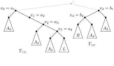
Figure 3: The operation of $\textsc{Split}(x)$.

Next, consider the forest $F:=T-\{x_{0},\dots,x_{r}\}$. This forest consists of $r+2$ (possibly empty) trees $A_{1},\dots,A_{r-1},L,R$ where $L$ and $R$ are the subtrees of $T$ rooted at the left and right child of $x$ in $T_{x}$ and, for each $i\in\{1,\dots,r-1\}$, $A_{i}$ is the subtree of $T$ rooted at the child $c_{i}\neq x_{i+1}$ of $x_{i}$ (if such a child exists, otherwise $A_{i}$ is empty). Make a binary search tree $T_{x}$ by replacing each of the $r+2$ external nodes of $T_{0}^{+}$ with the corresponding tree in $F$. Finally, let $T_{<x}$ be the subtree of $T_{x}$ rooted at the left child of $x$ and let $T_{>x}$ be the subtree of $T_{x}$ rooted at the right child of $x$ in $T_{x}$.

Lemma 15.

Let $T$ be any binary search tree, let $x$ be any node of $T$, and apply $\textsc{Split}(x)$ to obtain $T_{<x}$ and $T_{>x}$. Then $h(T_{<x})\le h(T)$ and $h(T_{>x})\le h(T)$.

Proof.

Note that for each node $z$ of $T_{<x}$, we have $V(P_{T_{<x}}(z))\subseteq V(P_{T}(z))$, so $d_{T_{<x}}(z)\le d_{T}(z)$. Therefore $h(T_{<x})\le h(T)$. The argument for $T_{>x}$ is symmetric. ∎

The following observation shows that there is a simple relationship between a node’s signature in $T$ before calling $\textsc{Split}(x)$ and its signature in $T_{<x}$ or $T_{>x}$.

Observation 16.

Let $T$, $x$, $x_{0},\dots,x_{r}$, $A_{1},\dots,A_{r-1},L,R$, $a_{1},\dots,a_{s}$, and $b_{1},\dots,b_{t}$ be defined as above. Then

1. for each $j\in\{1,\dots,s\}$ where $a_{j}=x_{i}$

   1. $\sigma_{T_{<x}}(a_{j})=1^{j-1}$, and

   2. $\sigma_{T_{<x}}(z)=1^{j-1},0,\sigma_{A_{i}}(z)$ for each $z\in V(A_{i})$;

2. for each $j\in\{1,\dots,t\}$ where $b_{j}=x_{i}$

   1. $\sigma_{T_{>x}}(b_{j})=0^{j-1}$, and

   2. $\sigma_{T_{>x}}(z)=0^{j-1},1,\sigma_{A_{i}}(z)$ for each $z\in V(A_{i})$;

3. $\sigma_{T_{<x}}(z)=1^{s},\sigma_{L}(z)$ for each $z\in V(L)$; and

4. $\sigma_{T_{>x}}(z)=0^{t},\sigma_{R}(z)$ for each $z\in V(R)$.

In particular, for any $z\in V(T)\setminus\{x\}$, $\sigma_{T_{<x}}(z)$ or $\sigma_{T_{>x}}(z)$ can be obtained from $\sigma_{T}(z)$ by deleting a prefix and replacing it with one of the $4\cdot h(T)$ strings in $\Pi:=\bigcup_{j=0}^{h(T)-1}\{0^{j},0^{j}1,1^{j},1^{j}0\}$.

3.3.2 $\textsc{MultiSplit}(x_{1},\dots,x_{c})$

From the $\textsc{Split}(x)$ operation we build the $\textsc{MultiSplit}(x_{1},\dots,x_{c})$ operation that takes as input a sequence of nodes $x_{1}<\cdots<x_{c}$ of $T$. For convenience, define $x_{0}=-\infty$ and $x_{c+1}=\infty$. The effect of $\textsc{MultiSplit}(x_{1},\dots,x_{c})$ is to split $T$ into a sequence of binary search trees $T_{0},\dots,T_{c}$ where, for each $i\in\{0,\dots,c\}$, $V(T_{i})=\{z\in V(T):x_{i}<z<x_{i+1}\}$.

The implementation of $\textsc{MultiSplit}(x_{1},\dots,x_{c})$ is straightforward divide-and-conquer: If $c=0$, then there is nothing to do. Otherwise, call $\textsc{Split}(x_{\lceil c/2\rceil})$ to obtain $T_{<x_{\lceil c/2\rceil}}$ and $T_{>x_{\lceil c/2\rceil}}$. Next, apply $\textsc{MultiSplit}(x_{1},\dots,x_{\lceil c/2\rceil-1})$ to $T_{<x_{\lceil c/2\rceil}}$ to obtain $T_{0},\dots,T_{\lceil c/2\rceil-1}$ and then apply $\textsc{MultiSplit}(x_{\lceil c/2\rceil+1},\dots,x_{c})$ to $T_{>x_{\lceil c/2\rceil}}$ to obtain $T_{\lceil c/2\rceil},\dots,T_{c}$.

The following lemma is immediate from Lemma 15.

Lemma 17.

Let $T$ be any binary search tree and apply $\textsc{MultiSplit}(x_{1},\dots,x_{c})$ to $T$ to obtain $T_{0},\dots,T_{c}$. Then $h(T_{i})\le h(T)$ for each $i\in\{0,\dots,c\}$.

3.3.3 $\textsc{Balance}(x,k)$

The $\textsc{Balance}(x,k)$ operation operates on the subtree $T_{x}$ of $T$ rooted at some node $x$ in $T$. The goal of this operation is to balance the size of all the subtrees rooted at nodes of depth $d_{T}(x)+k+1$ and contained in $T_{x}$. Refer to Figure 4.

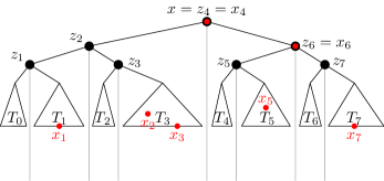
$\Downarrow$

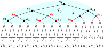
Figure 4: The operation of $\textsc{Balance}(x,k)$

If $|V(T_{x})|<2^{k}$, then this operation simply replaces $T_{x}$ with a perfectly balanced binary search tree containing $V(T_{x})$. Otherwise, let $Z:=\{z\in V(T_{x}):d_{T_{x}}(z)<k\}$. Call the $m\le 2^{k}-1$ elements of $Z$ $z_{1}<z_{2}<\cdots<z_{m}$ and, for convenience, define $z_{0}=-\infty$ and $z_{m+1}=\infty$.

Select the nodes $X:=\{x_{1},\dots,x_{2^{k}-1}\}$ of $T_{x}$ where each $x_{j}$ has rank $\lfloor j|V(T_{x})|/2^{k}\rfloor$ in $V(T_{x})$. The $\textsc{Balance}(x,k)$ operation will turn $T_{x}$ into a tree with a top part $\hat{T}_{0}$ that is a perfectly balanced binary search tree on $Z\cup X$. We now describe how this is done.

$T_{x}-Z$ is a forest consisting of $m+1\le 2^{k}$ trees $T_{0},\dots,T_{m}$. (Some of these trees may be empty.) Order $T_{0},\dots,T_{m}$ so that, for each $i\in\{0,\dots,m\}$ and each $x^{\prime}\in V(T_{i})$, $z_{i}<x^{\prime}<z_{i+1}$. For each $i\in\{0,\dots,m\}$, let $\{x_{i,1},\dots,x_{i,c_{i}}\}:=X\cap V(T_{i})$ where $x_{i,1}<\cdots<x_{i,c_{i}}$ and define $x_{i,0}:=z_{i}$ and $x_{i,c_{i}+1}:=z_{i+1}$. Note that for each $i\in\{0,\dots,m\}$, $c_{i}\le|X|\le 2^{k}-1$.

For each $i\in\{0,\dots,m\}$, apply $\textsc{MultiSplit}(x_{i,1},\dots,x_{i,c_{i}})$ to the tree $T_{i}$. As a result of these calls, we obtain sequences of trees $T_{i,0},\dots,T_{i,c_{i}}$ where, for each $i\in\{0,\dots,m\}$, each $j\in\{0,\dots,c_{i}\}$, and each $x^{\prime}\in V(T_{i,j})$, we have $x_{i,j}<x^{\prime}<x_{i,j+1}$. Note that if $c_{i}=0$ (i.e., if $X$ does not intersect $V(T_{i})$), then the result of this call is a single tree $T_{i,0}=T_{i}$. Observe that $\bigcup_{i=0}^{m}\bigcup_{j=0}^{c_{i}}V(T_{i,j})=V(T_{x})\setminus(Z\cup X)$.

Let $p:=|Z\cup X|$, let $s_{1}<\cdots<s_{p}$ denote the elements of $Z\cup X$ and define $s_{0}:=-\infty$ and $s_{p+1}:=\infty$. For each $\ell\in\{0,\dots,p\}$, let $i_{\ell}:=|Z\cap\{s_{1},\dots,s_{\ell}\}|$ and $j_{\ell}:=\ell-\max\{q\in\{1,\dots,\ell\}:s_{q}\in Z\}$ and let $A_{\ell}:=T_{i_{\ell},j_{\ell}}$. Then, for each $\ell\in\{0,\dots,p\}$ and each $x^{\prime}\in V(A_{\ell})$, we have $s_{\ell}<x^{\prime}<s_{\ell+1}$.

Now construct a perfectly balanced tree $\hat{T}_{0}$ with vertex set $V(\hat{T}_{0}):=\{s_{1},\dots,s_{p}\}=Z\cup X$. The tree $\hat{T}_{0}$ has $p+1$ external nodes $a_{0},\dots,a_{p}$. We obtain a new tree $T_{x}^{\prime}$ by replacing $a_{\ell}$ with $A_{\ell}$ for each $\ell\in\{0,\dots,p\}$ in $\hat{T}_{0}^{+}$. In the encompassing bulk tree $T$ we replace the subtree $T_{x}$ with $T_{x}^{\prime}$.

Lemma 18.

Let $T$ be any binary search tree, let $x$ be any node of $T$, and apply $\textsc{Balance}(x,k)$ to $T$ to obtain a new tree $T^{\prime}$. Then $h(T^{\prime})\le h(T)+1$.

Proof.

Since $\textsc{Balance}(x,k)$ only affects the subtree $T_{x}$ rooted at $x$, it suffices to show that $h(T_{x}^{\prime})\le h(T_{x})+1$. For each $i\in\{0,\dots,m\}$, $T_{i}$ is rooted at a depth-$k$ node of $T_{x}$, so $h(T_{i})\le h(T_{x})-k$. For each $\ell\in\{0,\dots,p\}$, $A_{\ell}$ is obtained by an application of MultiSplit to $T_{i}$ for some $i\in\{0,\dots,m\}$ so, by Lemma 17, $h(A_{\ell})\le h(T_{i})\le h(T_{x})-k$. Next, $|Z\cup X|\le|Z|+|X|\le 2^{k}-1+2^{k}-1<2^{k+1}-1$ and $\hat{T}_{0}$ is a perfectly balanced binary search tree of size $|\hat{T}_{0}|=|Z\cup X|$. Therefore $h(\hat{T}_{0})\le\lfloor\log|\hat{T}_{0}|\rfloor\le\lfloor\log(2^{k+1}-1)\rfloor=k$. Finally, $h(T_{x}^{\prime})\le h(\hat{T}_{0})+1+\max\{h(A_{\ell}):\ell\in\{0,\dots,p\}\}\le k+1+h(T_{x})-k\le h(T_{x})+1$. ∎

The following statement captures what we win after an application of $\textsc{Balance}(x,k)$ to a binary search tree.

Lemma 19.

Let $T$ be any binary search tree, let $x$ be any node of $T$, let $T_{x}$ be the subtree of $T$ rooted at $x$, and apply $\textsc{Balance}(x,k)$ to $T$ to obtain a new tree $T^{\prime}$. Then, for each $T^{\prime}$-descendant $z$ of $x$ with $d_{T^{\prime}}(z)=d_{T}(x)+k+1$, the subtree of $T^{\prime}$ rooted at $z$ has size at most $|T_{x}|/2^{k}$.

Proof.

Each such subtree is a subtree of $A_{\ell}$ for some $\ell\in\{0,\dots,p\}$. Now, $V(A_{\ell})\subset(x_{j},x_{j+1})$ for some $j\in\{1,\dots,2^{k-1}\}$. The values $x_{j}$ and $x_{j+1}$ have ranks $\lfloor j|T_{x}|/2^{k}\rfloor$ and $\lfloor(j+1)|T_{x}|/2^{k}\rfloor$ in the set $V(T_{x})$. Therefore, $|A_{\ell}|\le\lfloor(j+1)|T_{x}|/2^{k}\rfloor-\lfloor j|T_{x}|/2^{k}\rfloor-1\le|T_{x}|/2^{k}$. ∎

3.3.4 $\textsc{BulkBalance}(\theta,k)$

The ultimate restructuring operation in bulk trees is $\textsc{BulkBalance}(\theta,k)$. It calls Balance$(x,k)$ for each node $x$ of depth $\theta$ in $T$. (Note that this operation has no effect if there is no such node.) The following two lemmas are immediate consequences of Lemma 18 and Lemma 19, respectively.

Lemma 20.

Let $T$ be any binary search tree and apply the $\textsc{BulkBalance}(\theta,k)$ operation to obtain a new tree $T^{\prime}$. Then $h(T^{\prime})\le h(T)+1$.

Lemma 21.

Let $T$ be any binary search tree and apply the $\textsc{BulkBalance}(\theta,k)$ operation to obtain a new tree $T^{\prime}$. Let $x$ be any node of $T$ of depth $\theta$ and let $T_{x}$ be the subtree of $T$ rooted at $x$. Then, for each $T^{\prime}$-descendant $z$ of $x$ with $d_{T^{\prime}}(z)=\theta+k+1$, the subtree of $T^{\prime}$ rooted at $z$ has size at most $|T_{x}|/2^{k}$.

3.4 Bulk Tree Sequences

Let $k\ge 5$ be an integer and let $S_{0},\dots,S_{q}$ be a $1$-chunking sequence. We define a one-phase $k$-bulk tree sequence based on $S_{0},\dots,S_{q}$ to be a sequence $T_{0},\dots,T_{q}$ of binary search trees such that $T_{0}$ is an arbitrary binary search tree on node set $S_{0}$ and, for each $y\in\{0,\dots,q-1\}$, we have $h(T_{y})>y\cdot(k+1)$ and the tree $T_{y+1}$ is obtained from $T_{y}$ by applying

1. $\textsc{BulkBalance}(y\cdot(k+1),k)$, then

2. $\textsc{BulkInsert}(I)$ with $I:=S_{y+1}\setminus S_{y}$, and finally

3. $\textsc{BulkDelete}(D)$ with $D:=S_{y}\setminus S_{y+1}$.

Note that $V(T_{y})=S_{y}$ for each $y\in\{0,\dots,q\}$. The sequence is complete if $h(T_{q})\leq q\cdot(k+1)$.

For $k\geq 5$ and a $1$-chunking sequence $S_{1},\dots,S_{h}$, we define a $k$-bulk tree sequence based on $S_{1},\dots,S_{h}$ to be a sequence $T_{1},\dots,T_{h}$ of binary search trees satisfying: $T_{1}$ is a perfectly balanced binary search tree with $V(T_{1})=S_{1}$, and there exist indices $h_{1},h_{2},\dots,h_{\ell}$ with $1=h_{1}<h_{2}<\cdots<h_{\ell}=h$ such that $T_{h_{j}},T_{h_{j}+1},\dots,T_{h_{j+1}}$ is a complete one-phase $k$-bulk tree sequence based on $S_{h_{j}},S_{h_{j}+1},\dots,S_{h_{j+1}}$ for each $j\in\{1,\dots,\ell-2\}$, and $T_{h_{\ell-1}},T_{h_{\ell-1}+1},\dots,T_{h_{\ell}}$ is a (non-necessarily complete) one-phase $k$-bulk tree sequence based on $S_{h_{\ell-1}},S_{h_{\ell-1}+1},\dots,S_{h_{\ell}}$.

Note that if we fix the $1$-chunking sequence $S_{1},\dots,S_{h}$, the integer $k\ge 5$, and the starting perfectly balanced binary search tree $T_{1}$ with $V(T_{1})=S_{1}$, a $k$-bulk tree sequence based on $S_{1},\dots,S_{h}$ and starting with $T_{1}$ exists and is unique. It is obtained by a sequence of one-phase $k$-bulk tree sequences, where we start a new one-phase sequence as soon as the current one is complete.

This will not be needed until the final sections, but it is helpful to keep in mind that we will ultimately take $k=\max\left\{5,\left\lceil\sqrt{\log n/\log\log n}\right\rceil\right\}$ when considering a $k$-bulk tree sequence built for our $n$-vertex graph $G$, so that the expression $\mathcal{O}(k+k^{-1}\log n)$ (which appears many times in what follows), is $\omega(1)$ and $o(\log n)$.

Lemma 22.

Let $T_{0},\dots,T_{q}$ be a one-phase $k$-bulk tree sequence. Then, for each $y\in\{0,\dots,q\}$

1. $h(T_{y})\le h(T_{0})+2y$;

2. each subtree of $T_{y}$ rooted at a node of depth $y\cdot(k+1)$ has size at most $|T_{0}|\cdot 2^{-y(k-2)}$.

Proof.

The proof is by induction on $y$. For the base case $y=0$, both properties are trivial: (i) asserts that $h(T_{0})\le h(T_{0})$ and (ii) asserts that the subtree of $T_{0}$ rooted at the root of $T_{0}$ has size at most $|T_{0}|$.

For the inductive step, assume $y\ge 0$ and (i) holds for $T_{y}$. In order to get $T_{y+1}$, we first apply $\textsc{BulkBalance}(y\cdot(k+1),k)$ to $T_{y}$ to obtain $T^{\prime}$. By Lemma 20, we have $h(T^{\prime})\le h(T_{y})+1$. Let $I:=V(T_{y+1})\setminus V(T^{\prime})=V(T_{y+1})\setminus V(T_{y})$. Since $V(T_{y})$ $1$-chunks $V(T_{y+1})$ we know that $V(T^{\prime})$ $1$-chunks $I$. Next we apply $\textsc{BulkInsert}(I)$ to $T^{\prime}$ to obtain $T^{\prime\prime}$. Thus, by Lemma 11 we have $h(T^{\prime\prime})\le h(T^{\prime})+1$. Finally, we apply $\textsc{BulkDelete}(D)$ to $T^{\prime\prime}$ and obtain $T_{y+1}$, where $D:=V(T_{y})\setminus V(T_{y+1})$. By Lemma 13, we have $h(T_{y+1})\le h(T^{\prime\prime})$. Altogether we have

$$h(T_{y+1})\le h(T^{\prime\prime})\le h(T^{\prime})+1\le h(T_{y})+2\le h(T_{0})+2y+2=h(T_{0})+2(y+1).$$

Thus, (i) holds for $T_{y+1}$.

Next we establish (ii). Assume that (ii) holds for $T_{y}$. Thus, every subtree of $T_{y}$ rooted at a node of depth $y(k+1)$ has size at most $|T_{0}|\cdot 2^{-y(k-2)}$. Again, the first step when constructing $T_{y+1}$ from $T_{y}$ is to apply $\textsc{BulkBalance}(y(k+1),k)$ to $T_{y}$. By Lemma 21, this results in a tree $T^{\prime}$ in which every subtree rooted at a node of depth $(y+1)(k+1)$ has size at most $|T_{0}|\cdot 2^{-y(k-2)}\cdot 2^{-k}$. The second step is to apply $\textsc{BulkInsert}(I)$ to $T^{\prime}$ to obtain a new tree $T^{\prime\prime}$. By Lemma 12, every subtree of $T^{\prime\prime}$ rooted at a node of depth $(y+1)(k+1)$ has size at most $|T_{0}|\cdot 2^{-y(k-2)}\cdot 4\cdot 2^{-k}=2^{-y(k-2)+2-k}=2^{-(y+1)(k-2)}$. Finally, the third step is to perform $\textsc{BulkDelete}(D)$ on $T^{\prime\prime}$ to obtain $T_{y+1}$. Bulk deletion does not increase the size of any subtree, so every subtree of $T_{y+1}$ rooted at a node of depth $(y+1)(k+1)$ has size at most $|T_{0}|\cdot 2^{-(y+1)(k-2)}$, as desired. ∎

Corollary 23.

Let $T_{0},\dots,T_{q}$ be a one-phase $k$-bulk tree sequence. Then,

$$q\leq\left\lceil\tfrac{\log|T_{0}|}{k-2}\right\rceil.$$

Proof.

Arguing by contradiction, suppose that $q>\left\lceil\tfrac{\log|T_{0}|}{k-2}\right\rceil$. Note that when we take the logarithm of the upper bound in Lemma 22(ii) for $y:=\left\lceil\tfrac{\log|T_{0}|}{k-2}\right\rceil$, we have

$$\log|T_{0}|-\left\lceil\tfrac{\log|T_{0}|}{k-2}\right\rceil\cdot(k-2)\leq\log|T_{0}|-\tfrac{\log|T_{0}|}{k-2}\cdot(k-2)=0.$$

Thus, each subtree of $T_{y}$ rooted at a node of depth $y(k+1)$ has size at most

$$|T_{0}|\cdot 2^{-y(k-2)}\leq 1,$$

and hence $h(T_{y})\leq y(k+1)$, which violates the height condition in the definition of a one-phase $k$-bulk tree sequence. ∎

Lemma 24.

Let $T_{0},\dots,T_{q}$ be a complete one-phase $k$-bulk tree sequence, and let $r_{0}:=h(T_{0})-\log|T_{0}|$. Then, for each $y\in\{0,\dots,q\}$,

1. $|T_{0}|/4^{y}\le|T_{y}|$, and thus $\log|T_{0}|\le\log|T_{y}|+2y$;

2. $q=\mathcal{O}(k^{-1}\log|T_{y}|)$;

3. $h(T_{y})=\log|T_{y}|+r_{0}+\mathcal{O}(k^{-1}\log|T_{y}|)$; and

4. $h(T_{q})=\log|T_{q}|+\mathcal{O}(k+k^{-1}\log|T_{q}|)$.

Proof.

Let $I_{0},\dots,I_{q-1}$ and $D_{0},\dots,D_{q-1}$ be the sets so that $T_{y+1}$ is obtained from $T_{y}$ by rebalancing and then applying $\textsc{BulkInsert}(I_{y})$ and $\textsc{BulkDelete}(D_{y})$, for each $y\in\{0,\dots,q-1\}$. First, recall that by Lemma 12 and Lemma 14 we have $|T_{y+1}|\ge|T_{y}|/4$.

Iterating this starting with $T_{0}$ implies that $|T_{0}|/4^{y}\le|T_{y}|$, and thus $\log|T_{0}|\le\log|T_{y}|+2y$ for each $y\in\{0,\dots,q\}$, which proves (i).

By , we have $q\leq\left\lceil\frac{\log|T_{0}|}{k-2}\right\rceil$. Note that, for each $y\in\{0,\dots,q\}$, we have

$$q \le\tfrac{\log|T_{0}|}{k-2}+1\le\tfrac{\log|T_{y}|+2y}{k-2}+1\le\tfrac{\log|T_{y}|+2q}{k-2}+1, y\leq q$$ (by (i), and since )

and rewriting this yields (using that $$k\geq 5$$)

$$q \le\tfrac{\log|T_{y}|}{k-4}+\tfrac{k-2}{k-4}\leq\tfrac{k}{k-4}\cdot\tfrac{\log|T_{y}|}{k}+\tfrac{k-2}{k-4}$$

$$\leq 5\cdot\tfrac{\log|T_{y}|}{k}+3=\mathcal{O}(k^{-1}\log|T_{y}|),$$

which proves (ii). Now (iii) follows as for each $$y\in\{0,\dots,q\}$$, we have

$$h(T_{y}) \le h(T_{0})+2y$$ (by Lemma 22(i))

$$=\log|T_{0}|+2y+r_{0} r_{0}$$ (by definition of )

$$\le\log|T_{y}|+4y+r_{0}$$ (by (i))

$$\le\log|T_{y}|+4q+r_{0} y\le q$$ (since )

$$=\log|T_{y}|+\mathcal{O}(k^{-1}\log|T_{y}|)+r_{0}.$$ (by (ii))

(iv) follows from

$$h(T_{q}) \le(k+1)q$$ (since the sequence is complete)

$$\le(k+1)\left(\tfrac{\log|T_{0}|}{k-2}+1\right)$$ (by )

$$=\left(\tfrac{k+1}{k-2}\right)\cdot\log|T_{0}|+(k+1)$$

$$\le\left(\tfrac{k+1}{k-2}\right)\cdot(\log|T_{q}|+2q)+(k+1)$$ (by (i))

$$=\log|T_{q}|+\tfrac{3}{k-2}\log|T_{q}|+2\cdot\tfrac{k+1}{k-2}q+k+1$$

$$=\log|T_{q}|+\mathcal{O}(k+k^{-1}\log|T_{q}|). \tfrac{k+1}{k-2}\leq\tfrac{6}{3}$$ (as , and by (ii))

∎

The following lemma shows that trees in a bulk tree sequence are balanced at all times:

Lemma 25.

Let $T_{1},\dots,T_{h}$ be a $k$-bulk tree sequence and let $y\in\{1,\dots,h\}$. Then

$$h(T_{y})\le\log|T_{y}|+\mathcal{O}(k+k^{-1}\log|T_{y}|).$$

Proof.

By the definition of a $k$-bulk tree sequence, $T_{1}$ is a perfectly balanced binary tree so $h(T_{1})=\lceil\log|T_{1}|\rceil$ and the statement is satisfied for $y=1$. Let $h_{1},h_{2},\dots,h_{\ell}$ be indices with $1=h_{1}<h_{2}<\cdots<h_{\ell}=h$ such that $T_{h_{j}},\dots,T_{h_{j+1}}$ is a complete one-phase $k$-bulk tree sequence for each $j\in\{1,\dots,\ell-2\}$, and $T_{h_{\ell-1}},\dots,T_{h_{\ell}}$ is a one-phase $k$-bulk tree sequence. Let $Y:=\{h_{1},h_{2},\dots,h_{\ell-1}\}$. For $y\in Y\setminus\{1\}$, Lemma 24(iv) implies that $T_{y}$ satisfies the conditions of the lemma.

All that remains is to show that the conditions of the lemma are satisfied for each $y\in\{1,\dots,h\}\setminus Y$. To show this, let $y_{0}:=\max\{y^{\prime}\in Y:y^{\prime}<y\}$. That is, $T_{y_{0}}$ is the tree that began the one-phase $k$-bulk tree sequence in which $T_{y}$ takes part. In this case, Lemma 24(iii) implies that

$$h(T_{y})\le\log|T_{y}|+\mathcal{O}(k^{-1}\log|T_{y}|)+h(T_{y_{0}})-\log|T_{y_{0}}|.$$

Thus, all that is required is to show that $r_{0}:=h(T_{y_{0}})-\log|T_{y_{0}}|\in\mathcal{O}(k+k^{-1}\log|T_{y}|)$ so that is what we do. Note that by Lemma 24(ii) we have $y-y_{0}=\mathcal{O}(k^{-1}\log|T_{y}|)$.