Lagrangian schemes for Wasserstein Gradient Flows

Lagrangian schemes for Wasserstein Gradient Flows

Abstract.

This paper reviews different numerical methods for specific examples of Wasserstein gradient flows: we focus on nonlinear Fokker-Planck equations, but also discuss discretizations of the parabolic-elliptic Keller-Segel model and of the fourth order thin film equation. The methods under review are of Lagrangian nature, that is, the numerical approximations trace the characteristics of the underlying transport equation rather than solving the evolution equation for the mass density directly. The two main approaches are based on integrating the equation for the Lagrangian maps on the one hand, and on solution of coupled ODEs for individual mass particles on the other hand.

1. Introduction

In most general terms, $L^{2}$-Wasserstein gradient flows are evolution equations for a time-dependent probability density $\rho_{(\cdot)}:[0,T]\times\Omega\to{\mathbb{R}}_{\geq 0}$ on a domain $\Omega\subset\mathbb{R}^{d}$ that can be written as follows:

(1) $$\partial_{t}\rho_{t}+\operatorname{div}(\rho_{t}\,{\mathbf{v}}_{t})=0,\quad\text{with}\quad{\mathbf{v}}_{t}=-\left[\nabla\frac{\delta\mathcal{E}}{\delta\rho}(\rho_{t})\right],$$

subject to no-flux boundary conditions. In equation (1) the probability density $\rho$ is transported along a time-dependent gradient vector field ${\mathbf{v}}_{t}:\Omega\to{\mathbb{R}}^{d}$; and the pressure generating that vector field depends on $\rho$ through the variational derivative of a free energy functional $\mathcal{E}$. In this chapter, we shall review Lagrangian methods for computing the solutions of (1).

1.1. Examples for (1)

The most prominent example of the form (1) is the linear heat equation $\partial_{t}\rho_{t}=\Delta\rho_{t}$. Indeed, choosing $\mathcal{E}$ as Boltzmann’s entropy functional, $\mathcal{E}(\rho)=\mathcal{H}_{1}(\rho):=\int_{\Omega}\rho\log\rho\,\mathrm{d}x$, one obtains:

$$\frac{\delta\mathcal{H}_{1}}{\delta\rho}(\rho_{t})=\log\rho_{t},\quad\text{and thus}\quad\partial_{t}\rho_{t}=\operatorname{div}(\rho_{t}\nabla\log\rho_{t})=\Delta\rho_{t}.$$

Note that this is a hydrodynamical view on the heat equation, which is complementary to the more classical understanding in probabilistic terms as stochastic motion of Brownian particles.

Among the many further evolution equations of the form (1), there are non-linear and non-local Fokker-Planck equations,

(2) $$\partial_{t}\rho_{t}=\Delta\Phi(\rho_{t})+\operatorname{div}\big{(}\rho_{t}\,[\nabla V+\rho_{t}\ast\nabla W]\big{)},$$

where $\Phi:{\mathbb{R}}_{\geq 0}\to{\mathbb{R}}_{\geq 0}$ is a nonlinearity subject to certain conditions (e.g., $\Phi(\rho)=\rho^{m}$ with arbitary $m>0$ is allowed), $V\in C^{2}(\Omega)$ is an external potential, and $W\in C^{2}({\mathbb{R}}^{d})$ represents the potential of a non-local inter-particle interaction. The corresponding entropy functional is

(3) $$\mathcal{E}(\rho)=\mathcal{H}_{h,V,W}(\rho):=\int_{\Omega}\big{[}h(\rho)+\rho V+\frac{1}{2}\rho(W\ast\rho)\big{]}\,\mathrm{d}x,$$

with an entropy density $h:{\mathbb{R}}_{\geq 0}\to{\mathbb{R}}$ such that $\rho h^{\prime\prime}(\rho)=\Phi^{\prime}(\rho)$. In the variational context, equation (2) is augmented with the natural boundary conditions, which are no-flux,

(4) $$\rho\nabla\big{[}h^{\prime}(\rho)+V+W*\rho\big{]}\cdot{\boldsymbol{\nu}}=0\quad\text{ for all }x\in\partial\Omega,\,t>0,$$

with ${\boldsymbol{\nu}}$ the unit outwards normal to the boundary of $\Omega$. For an overview on the vast field of applications of porous medium or filtration equations, which are (2) with $V\equiv 0$ and $W\equiv 0$, we refer to the book of Vazquez [Váz07]. More recently, a rich theory has been developed for (2) with irregular potentials $W$. A case of particular interest is the parabolic-elliptic Keller-Segel model, which is (2) with linear diffusion $\Phi(r)=r$, with $V\equiv 0$, and $W$ given by the Newtonian potential, that is $W(z)=\frac{1}{2\pi}\log|z|$ in dimension $d=2$, see [DP04, BDP06, BCC08, BCC12, CCY19] and the references therein. Complementary to that, a solution theory has been developed, see e.g. [CDF⁺11], for quite general interaction potentials $W$, even in the absense of diffusion, $\Phi\equiv 0$. Prominent applications are in studies of the collective dynamics of bird flocks or fish schools, see for example [BCL09, HB10, CDF⁺11, BGL12, BCLR13a, BCLR13b], but such equations also find applications in physics, for example for granular media [Tos00, CMV03, LT04, CMV06] or in material sciences e.g [HP05].

Examples of fourth order equations of type (1) include

(5) $$\partial_{t}\rho_{t}+\operatorname{div}(\rho_{t}\nabla\Delta\rho_{t})=0,\quad\text{and}\quad\partial_{t}\rho_{t}+\operatorname{div}\left(\rho_{t}\nabla\frac{\Delta\sqrt{\rho_{t}}}{\sqrt{\rho_{t}}}\right)=0.$$

These equations are, respectively, known as the thin film equation with linear mobility from lubrication theory [Ber98], and the quantum drift diffusion equation from semi-conductor modeling [Jün09]. The corresponding free energy functionals are the Dirichlet energy, and the Fisher information,

(6) $$\mathcal{E}_{\text{Dirichlet}}(\rho)=\frac{1}{2}\int_{\Omega}|\nabla\rho|^{2}\,\mathrm{d}x\quad\text{and}\quad\mathcal{E}_{\text{Fisher}}(\rho)=\int_{\Omega}|\nabla\log\rho|^{2}\rho\,\mathrm{d}x.$$

Notation and Basic concepts.- For definiteness, let $\Omega\subset{\mathbb{R}}^{d}$ be a bounded and convex domain throughout this chapter. Let us denote by $\mathcal{P}(\Omega)$ the set of probability measures with support on the open set $\Omega$. Further, recall the notation of push-forward of a density $\rho:\Omega\to{\mathbb{R}}$ through a map $T:\Omega\to\Omega$:

$$T\#\rho=\frac{\rho}{\det\operatorname{D}T}\circ T^{-1}.$$

There are several possible definitions of the euclidean transport distance ${\mathbf{W}_{2}}$ between two probability measures, the most robust being the infimum in the Kantorovich problem:

(7) $${\mathbf{W}_{2}}(\rho,\eta)^{2}=\inf_{\gamma\in\Gamma(\rho,\eta)}\int_{\Omega\times\Omega}|x-y|^{2}\,\mathrm{d}\gamma(x,y),$$

where $\Gamma(\rho,\eta)$ is the set of all couplings between $\rho$ and $\eta$, that is,

$$\Gamma(\rho,\eta)=\left\{\gamma\in{\mathcal{P}}(\Omega\times\Omega)\,\middle|\,\forall A,B\subseteq\Omega:\gamma[A\times\Omega]=\rho[A],\,\gamma[\Omega\times B]=\eta[B]\right\}.$$

For the Lagrangian approach discussed here, we shall use Monge’s original definition, which is equivalent to the one above at least if $\rho$ is absolutely continuous, see [Bre91]:

$${\mathbf{W}_{2}}(\rho,\eta)^{2}=\inf_{T:\eta=T\#\rho}\int_{\Omega}|T(x)-x|^{2}\rho(x)\,\mathrm{d}x.$$

We refer to [Vil03b, San15] for the basics of optimal transport concepts. There also exists an Eulerian approach to optimal transport introduced by Benamou and Brenier [BB00], we will postopone its dicussion to the last section where we will make use of it.

1.2. Lagrangian formulation of (1)

The transport character of (1) calls for a Lagrangian formulation of the dynamics. We adopt the microscopic picture of particles that move along the vector field ${\mathbf{v}}$, which is influenced by themselves through the induced change of the macroscopic particle density $\rho$. For definiteness, let $\Theta\subset{\mathbb{R}}^{d}$ be a reference domain and $\theta\in{\mathcal{P}}(\Theta)$ be a reference probability density. A canonical choice is $\Theta=\Omega$ and $\theta=u_{0}$, the initial condition, but we shall discuss further possible choices below. The Lagrangian map $X_{(\cdot)}:[0,T]\times\Theta\to\Omega$ is associated to a solution $\rho_{t}$ of (1), such that $t\mapsto X_{t}(\xi)\in\Omega$ describes the trajectory of a particle with label $\xi\in\Theta$. That is,

(8) $$\partial_{t}X_{t}={\mathbf{v}}_{t}\circ X_{t}.$$

Provided that $X_{0}$ is chosen such that $X_{0}\#\theta=\rho_{0}$, i.e., $X_{0}$ realizes the initial density, then

$$\rho_{t}=X_{t}\#\theta$$

at any $t\in[0,T]$. Next we introduce

$$\mathcal{E}^{\#}(X):=\mathcal{E}(X\#\theta),$$

and use that for every diffeomorphism $\bar{X}:\Theta\to\Omega$,

$$\frac{1}{\theta}\frac{\delta\mathcal{E}^{\#}}{\delta X}(\bar{X})=\nabla\frac{\delta\mathcal{E}}{\delta\rho}(\bar{X}\#\theta)\circ\bar{X},$$

see Lemma 1 in the appendix. Then the probability density $\rho_{t}$ can be completely eliminated from the evolution equation, leading to a closed system for $X$ alone,

(9) $$\partial_{t}X_{t}=-\frac{1}{\theta}\frac{\delta\mathcal{E}^{\#}}{\delta X}(X_{t}).$$

Note that equation (1) and (9) are equivalent for smooth solutions with everywhere-positive $\rho_{t}$.

1.3. Two gradient flow structures

We briefly recall the basic terminology of gradient flows: on a Riemannian manifold ${\mathcal{M}}$ with a local scalar product $\langle\cdot,\cdot\rangle_{x}$, the gradient flow of a function $F\in C^{2}({\mathcal{M}})$ is formed by solutions $x_{(\cdot)}:[0,T]\to{\mathcal{M}}$ to

(10) $$\frac{d}{dt}x_{t}=-\operatorname{grad}_{\mathcal{M}}F(x_{t}),$$

where the gradient $\operatorname{grad}_{\mathcal{M}}F(x)$ of $F$ at $x\in{\mathcal{M}}$ is the unique element $v\in\mathrm{T}_{x}{\mathcal{M}}$ in ${\mathcal{M}}$’s tangent space at $x$ with $\langle v,w\rangle_{x}=\operatorname{D}F(x)[w]$ for all $w\in\mathrm{T}_{x}{\mathcal{M}}$. With this definition of the gradient, it is clear that any solution $x_{(\cdot)}$ to (10) descends in $F$’s potential landscape “as fast as possible” in the sense that a curve $x_{(\cdot)}:[0,T]\to{\mathcal{M}}$ is a solution if and only if at each instance of time $t\in[0,T]$, its tangent vector $dx_{t}/dt\in\mathrm{T}_{x}{\mathcal{M}}$ minimizes among all $v\in\mathrm{T}_{x}{\mathcal{M}}$ the following expression:

(11) $$\frac{1}{2}\langle v,v\rangle_{x_{t}}+\operatorname{D}F(x_{t})[v].$$

There are two ways in which (1) can be considered as a gradient flow.

The first is obvious from the Lagrangian formulation (9), which is directly identified as an $L^{2}$-gradient flow of $\mathcal{E}^{\#}$ on the space of Lagrangian maps. Here the role of the manifold ${\mathcal{M}}$ is played by $L^{2}_{\theta}(\Theta;\Omega)$, the linear space of measurable maps $X:\Theta\to\Omega$, whose tangent space at any point consists of square integrable vector fields ${\mathbf{v}}:\Theta\to{\mathbb{R}}^{d}$, and is equipped with the scalar product

$$\langle{\mathbf{v}},{\mathbf{w}}\rangle_{\theta}=\int_{\Theta}{\mathbf{v}}\cdot{\mathbf{w}}\,\theta\,\mathrm{d}\xi.$$

While this $L^{2}$-gradient flow structure is easily understood, the second structure introduced in the seminal paper by Otto [Ott01a] is more subtle: (1) is a metric gradient flow of $\mathcal{E}$ in the $L^{2}$-Wasserstein distance. Here, the role of the manifold ${\mathcal{M}}$ is played by the space of probability measures ${\mathcal{P}}(\Omega)$. The rigorous construction of the Wasserstein tangent space at some $\rho\in{\mathcal{P}}(\Omega)$ amounts to identifying — via the continuity equation — tangent vectors with elements in the closure of all gradient vector fields $\nabla\varphi:\Omega\to{\mathbb{R}}^{d}$ with $\varphi\in C^{\infty}_{c}(\Omega)$ in the $\rho$-weighted $L^{2}$-norm. Less rigorously and more intuitively: if $(\rho_{t})_{t\in[0,T]}$ is some sufficiently regular curve in ${\mathcal{P}}(\Omega)$, then at each $t\in[0,T]$, there is an essentially unique gradient vector field ${\mathbf{v}}_{t}=\nabla\varphi_{t}$ such that $\partial_{t}\rho_{t}+\operatorname{div}(\rho_{t}{\mathbf{v}}_{t})=0$. Inside that framework, the analogue of the local scalar product between two tangent vectors, identified with $\nabla\varphi$ and $\nabla\psi$, respectively, amounts to

(12) $$\langle\nabla\varphi,\nabla\psi\rangle_{\rho}:=\int_{\Omega}\nabla\varphi\cdot\nabla\psi\,\rho\,\mathrm{d}x.$$

In this context, the $L^{2}$-Wasserstein distance ${\mathbf{W}_{2}}(\rho^{0},\rho^{1})$ between $\rho^{0},\rho^{1}\in{\mathcal{P}}(\Omega)$ can be introduced as shortest connecting curve $(\rho^{s})_{0\leq s\leq 1}$ from $\rho^{0}$ to $\rho^{1}$,

(13) $${\mathbf{W}_{2}}(\rho^{0},\rho^{1})=\inf_{(\rho^{s})_{0\leq s\leq 1}}\left\{\int_{0}^{1}\langle\nabla\psi^{s},\nabla\psi^{s}\rangle_{\rho^{s}}\,\mathrm{d}s\,\middle|\,\partial_{s}\rho^{s}+\operatorname{div}(\rho^{s}\nabla\psi^{s})=0\right\}.$$

With this dictionary at hand, it is now straight-forward to conclude that (1) is the analogue of (10), and in particular, ${\mathbf{v}}_{t}$ is identified with the gradient of $\mathcal{E}$ at $\rho_{t}$ with respect to the local scalar product (12). In analogy to the situation on the Riemannian manifold, we define the gradient in the Wasserstein metric (with a certain abuse of notation) by

(14) $$\operatorname{grad}_{\mathbf{W}_{2}}\mathcal{E}=\nabla\frac{\delta\mathcal{E}}{\delta\rho},$$

so that (1) becomes

$$\partial_{t}\rho_{t}=\operatorname{div}\big{(}\rho_{t}\operatorname{grad}_{\mathbf{W}_{2}}\mathcal{E}(\rho_{t})\big{)}.$$

We stress that this discussion is very formal. The introduction of the $L^{2}$-Wasserstein distance ${\mathbf{W}_{2}}$ via (13) is full of technical subtleties, see [BB00]. Moreover, the functionals $\mathcal{E}$ of interest are far from being differentiable, but typically just lower semi-continuous, which makes it impossible to define a gradient in a simple way as in (14).

There are fully rigorous approaches to understanding solutions to (1) as being of steepest descent, the most prominent being the theory of metric gradient flows developed by Ambrosio et al [AGS08]. There, one completely avoids the scalar product (12) and defines ${\mathbf{W}_{2}}$ as a global metric on ${\mathcal{P}}(\Omega)$. Accordingly, the metric gradient flow is not formulated in differential terms, but instead is characterized by variational principles that are formally related to (11) above, that is, to consider curves $t\mapsto\rho_{t}$ in ${\mathcal{P}}(\Omega)$ whose motion — now measured in ${\mathbf{W}_{2}}$ — is such that it decreases the functional $\mathcal{E}$ as fast as possible. This can be formulated in robust variational ways, like the energy dissipation equality, or the evolutionary variational inequalities.

Unfortunately, this approach is very abstract, and it has surprising limitations in view of applicability to concrete evolution equations of type (1). While the non-linear Fokker-Planck equation (2) fits well into the framework of [AGS08], this is not the case for the fourth order equations (5). Therefore, we shall adopt a more practical view on Wasserstein gradient flows here, which is centered around the question: “What are the properties implied on solutions to (1) by the theory, and how can they be used for the design of numerical schemes?”

2. Benefit from the gradient flow structures

As indicated above, we shall not go into details of the theory of metric gradient flows but only summarize results and techniques that are of interest for the design and analysis of numerical schemes.

2.1. Existence of solutions by minimizing movements

Knowing that (1) is (at least formally) a gradient flow in the Wasserstein metric for a reasonable functional $\mathcal{E}$, one almost automatically obtains the existence of curves $\rho_{(\cdot)}$ in ${\mathcal{P}}(\Omega)$ that realize the principle of steepest descent indicated in (11). The general approach to their construction goes via the celebrated variational form of the implicit Euler discretization in time, commonly referred to as minimizing movement scheme. More specifically, for a given time step size ${\Delta t}>0$, a sequence $(\rho_{\Delta t}^{n})_{n=0}^{\infty}$ of $\rho_{\Delta t}^{n}\in{\mathcal{P}}(\Omega)$ such that $\rho_{\Delta t}^{n}$ approximates the density $\rho(n{\Delta t})$ of the true solution at time $t=n\tau$ are obtained as follows: one starts from the initial condition $\rho_{\Delta t}^{0}:=\rho_{0}$, and then one defines each $\rho_{\Delta t}^{n}$ for $n=1,2,\ldots$ inductively as minimizer of

(15) $$\rho\mapsto\frac{1}{2{\Delta t}}{\mathbf{W}_{2}}(\rho,\rho_{\Delta t}^{n-1})^{2}+\mathcal{E}(\rho).$$

Note that (15) can be formally derived by integrating (11) in time from $t=(n-1)\tau$ to $t=n\tau$ along a solution $\rho_{(\cdot)}$, and approximating the integral over the metric term by the distance. Unqiue solvability of (15) follows under the typical hypotheses from calculus of variations.

By abstract arguments, the time-interpolated $\rho_{\Delta t}^{n}$ have accumulation points in the space of continuous curves on ${\mathcal{P}}(\Omega)$ for ${\Delta t}\to 0$. The difficulty is then to show that these limit curves are indeed solutions to (1) in some sense. This has been shown for the Fokker-Planck equation (2) and for the thin film and QDD equations (5), see [JKO98, Ott98, Ott01b, BCC08, BCC12, GST09, MMS09, CDF⁺11]. This method of approximation in time is so reliable that it is the basis for essentially all numerical schemes for gradient flows. We mention that variational discretizations in time of higher order have been developed recently [LT17, MP19, Pla19], but are not yet widely used.

2.2. Long time asymptotics from displacement convexity

Some functionals $\mathcal{E}$ of interest happen to be $\lambda$-uniformly displacement convex in the sense of McCann [McC97]: that is, there is a $\lambda\in{\mathbb{R}}$ such that for any “reasonable” unit speed geodesic $(\eta_{s})_{s\in[0,\sigma]}$ in $({\mathcal{P}}(\Omega),{\mathbf{W}_{2}})$, the real function $s\mapsto\mathcal{E}(\eta_{s})$ has second derivative bounded below by $\lambda$. This is true for instance for the entropy functional $\mathcal{H}_{h,V,W}$ under the hypotheses that $h$ satisfies the McCann condition:

1. $h$ is convex with $h(0)=0$, and $s\mapsto s^{d}h(s^{-d})$ is convex and non-increasing,

2. $W$ is convex, and

3. $V$ is $\lambda$-uniformly convex, that is $\nabla^{2}V\geq\lambda{\mathbf{1}}$.

For Wasserstein gradient flows of such functionals, one obtains interesting consequences on the long-time asymptotics of solutions $\rho_{(\cdot)}$.

A first implication of $\lambda$-uniform displacement convexity is $\lambda$-uniform contractivity of the flow: for any two solutions $\rho_{(\cdot)}$ and $\eta_{(\cdot)}$ the map

(16) $$t\mapsto e^{\lambda t}{\mathbf{W}_{2}}(\rho_{t},\eta_{t})$$

is non-increasing in time. Note that for $\lambda>0$, this implies mutual attraction of solutions at exponential rate in time, for $\lambda<0$, it estimates the speed of divergence from each other. In any case, monotonicity of (16) implies uniqueness. If $\lambda>0$, then it follows from contractivity that (1) has a unique stationary solution $\rho_{*}$, which coincides with the unique minimizer of $\mathcal{E}$, and any solution $\rho_{(\cdot)}$ to (1) converges to $\rho_{*}$ exponentially fast:

(17) $$t\mapsto e^{\lambda t}{\mathbf{W}_{2}}(\rho_{t},\rho_{*})\quad\text{and}\quad t\mapsto e^{\lambda t}\big{(}\mathcal{E}(\rho_{t})-\mathcal{E}(\rho_{*})\big{)}$$

are non-increasing in $t\geq 0$. The estimates in (17) have been the key to study the long-time asymptotics of various PDEs of type (1), see e.g. [Ott01b, CMV03, CMV06, MMS09, CDF⁺11, BCC12].

Preserving convexity is one of the central interests in designing numerical methods for (1). If ${\mathcal{P}}(\Omega)$ is approximated by a finite-dimensional metric space, and $\mathcal{E}$ is discretized thereon such that it has the same modulus $\lambda$ of convexity, then the discretized gradient flow is automatically asymptotic preserving in the sense that solutions share the monotonicities (16) and (17). Moreover, from the computational perspective, a very useful consequence of $\lambda$-uniform displacement convexity is that the minimization problem (15) is uniformly convex as well, with modulus $\lambda^{\prime}:=\frac{1}{\tau}+\lambda$.

2.3. Polyconvexity from displacement convexity

A benefit from the gradient flow structure of (1) in ${\mathbf{W}_{2}}$ is that the evolution (9) for the Lagrangian map $X$ is a gradient flow as well: one replaces the space of probability measures with the intricate Wasserstein distance by a space of maps, equipped with the much easier $L^{2}$-structure. The construction of solutions via minimizing movements carries over from (15): a sequence of maps $(X_{\tau}^{n})_{n=0}^{\infty}$ is inductively obtained by minimizing

(18) $$\frac{1}{2{\Delta t}}\|X-X_{\Delta t}^{n-1}\|_{L^{2}_{\theta}}^{2}+\mathcal{E}^{\#}(X).$$

In contrast to (15), this problem is much easier to solve in practice, since it does not involve the calculation of the Wasserstein distance, but only of an $L^{2}$-norm.

There is, however, a price to pay. An obvious drawback is that the transformed functionals $\mathcal{E}^{\#}$ typically attain a much more complicated form than their respective originals $\mathcal{E}$. For instance, in the comparatively easy case of the relative entropy $\mathcal{H}_{h,V,W}$ from (3), one obtains

(19) $$\begin{split}\mathcal{H}_{h,V,W}^{\#}(X)&=\int_{\Theta}\left[h^{\#}\left(\frac{\det\operatorname{D}X}{\theta}\right)+V(X)\right]\theta\,\mathrm{d}\xi\\ &\quad+\int_{\Theta}\int_{\Theta}W\big{(}X(\xi)-X(\xi^{\prime})\big{)}\theta(\xi)\theta(\xi^{\prime})\,\mathrm{d}\xi\,\mathrm{d}\xi^{\prime},\end{split}$$

with the definition

(20) $$h^{\#}(s)=sh(s^{-1}).$$

Another, more subtle difficulty arises in any space dimension $d>1$: the correspondence $X\mapsto X\#\theta$ is not an isometry between the $L^{2}$-distance on injective monotone maps and the Wasserstein distance on densities. In fact, that correspondence is highly non-unique — for any given sufficiently regular $\rho$, there are infinitely many genuinely different maps $X$ such that $X\#\theta=\rho$ — and there is no “universal normalization” of the $X$’s such that ${\mathbf{W}_{2}}(X_{0}\#\theta,X_{1}\#\theta)=\|X_{0}-X_{1}\|_{L^{2}(\theta)}$ would be true in general. In particular, the linear interpolation between $X_{0}$ and $X_{1}$ has typically little to do with the Wasserstein geodesic connecting $X_{0}\#\theta$ to $X_{1}\#\theta$. Therefore, displacement convexity of $\mathcal{E}$ does usually not imply any flat convexity of $\mathcal{E}^{\#}$, and contractivity of the gradient flow (1) with respect to ${\mathbf{W}_{2}}$ does not imply contractivity of (9) with respect to $L^{2}$. What remains from displacement convexity is polyconvexity: in the situation above, the functional in (19) is indeed polyconvex if the corresponding $\mathcal{H}_{h,V,W}$ is $\lambda$-uniformly displacement convex with $\lambda\geq 0$. We remark that the correspondence between (1) and (9) has first been pointed out — at least in the special case of the Fokker-Planck equation (2) — by Evans et al [ESG05], where they also propose to solve (9) by the implicit time discretization (18), based on the polyconvexity of the functional $\mathcal{E}^{\#}$, It was then shown later [ALS06] that, at least for $\mathcal{E}=\mathcal{H}_{h,0,0}$, there is indeed a one-to-one correspondence between the variational problems (15) and (18), i.e., under suitable hypotheses on the initial condition $\rho_{0}$, the discrete iterates coincide, $\rho_{\tau}^{n}=X_{\tau}^{n}\#\rho_{0}$. This fact was later used for constructing maps joining particular densites with given Jacobians, see [CL10].

In summary: The gradient flow structures lead to natural time-discretizations of (1) that are in variational form, see either equation (15) or equation (18). These variational problems are even strictly geodesically convex or polyconvex, respectively, if $\mathcal{E}$ happens to be $\lambda$-uniformly displacement convex in the sense of McCann. Preserving that convexity also under spatial discretization leads to schemes that replicate contractivity (16) and convergence to equilibrium (17), thus reproducing the correct long time asymptotics. Moreover, discretizing the Lagrangian form (9) of the dynamics automatically ensures properties like mass conservation and non-negativity.

3. 1D Wasserstein using the inverse distribution functions

In space dimension $d=1$ the conceptual difference between performing a minimization in (15) on a discretized set of Lagrangian maps, and discretizing the Lagrangian equations directly is little. The reason is the isometry between the Wasserstein space over an interval $I=[a,b]\subset{\mathbb{R}}$, and the $L^{2}$-space of inverse distribution functions with values in $I$.

3.1. The inverse distribution function

We recall the basic definitions and relations:

• To each $\rho\in{\mathcal{P}}(I)$, one associates the cumulative distribution function $F_{\rho}:I\to\Theta$ via $F_{\rho}(x)=\rho[[a,x]]$, where $\Theta=[0,1]$. By outer regularity, $F_{\rho}$ is non-decreasing and càdlàg. It is strictly increasing on the support of $\rho$, and it is continuous if $\rho$ is an absolutely continuous measure.

• By the usual construction, one obtains a unique non-decreasing càdlàg right inverse $X_{\rho}:\Theta\to I$ of $F_{\rho}$, called $\rho$’s inverse distribution function. $X_{\rho}$ is a genuine inverse if $\rho$ is absolutely continuous and has support $I$.

• The definition directly implies that, with $\theta$ being the Lebesgue measure on $\Theta=[0,1]$,

  (21) $$\rho=X_{\rho}\#\theta,$$

  and $X_{\rho}$ is the only non-decreasing càdlàg function $X:\Theta\to I$ with that property. Consequently, if $\rho$ is absolutely continuous with an everywhere positive and continuous density function, then $X_{\rho}$ is continuously differentiable with

  (22) $$\rho\circ X_{\rho}=\frac{1}{\partial_{\xi}X_{\rho}}.$$

  This relation generalizes in the obvious way when $\rho$’s density has isolated points of discontinuity.

• The association $\rho\mapsto X_{\rho}$ is an isometry in the following sense:

  $${\mathbf{W}_{2}}(\rho,\eta)=\|X_{\rho}-X_{\eta}\|_{L^{2}([0,1])}.$$

  Particularly, the space $({\mathcal{P}}(I),{\mathbf{W}_{2}})$ is flat, and Wasserstein geodesics are given through linear interpolation of the respective inverse distribution functions.

The following equivalence is obvious: if a sequence $(\rho_{\Delta t}^{n})_{n=0}^{\infty}$ of $\rho_{\Delta t}^{n}\in{\mathcal{P}}(I)$ is minimal for (15), then the sequence $(X_{\Delta t}^{n})_{n=0}^{\infty}$ of respective inverse distribution functions $X_{\tau}^{n}:=X_{\rho_{\tau}^{n}}$ is minimal in (18); and if a sequence $(X_{\Delta t}^{n})_{n=0}^{\infty}$ of non-decreasing càdlàgfunctions $X_{\Delta t}^{n}:\Theta\to I$ is minimal in (18), then the sequence $(\rho_{\Delta t}^{n})_{n=0}^{\infty}$ of respective densities $\rho_{\Delta t}^{n}:=X_{\Delta t}^{n}\#\theta$ is minimal in (15). Moreover, if $\mathcal{E}$ is $\lambda$-uniformly displacement convex, then the minimization problem (18) is convex of modulus $\frac{1}{\tau}+\lambda$. In fact contraction estimates in one dimension can be obtained in this formulation [CT04, LT04, BCC08]. This formulation can also be used to obtain well-posedness of solutions in the theoretical setting [CHR20] even when blow-up of the densities can occur.

3.2. Discretization

Lagrangian numerical schemes for solution of the one-dimensional Fokker-Planck, thin film and QDD equations have been devised by various authors, see e.g. [GT06b, GT06a, BCC08, WW10, CN10, CRW16]. Below, we review the ansatz made in [MO14, OM17, MO17, Osb17].

As ansatz space ${\mathcal{X}_{\mathbf{\xi}}}$ for the inverse distribution functions $X$, we choose the continuous and strictly increasing functions $X:\Theta\to I$ that are piecewise linear with respect to a given partition ${\mathbf{\xi}}=(\xi_{k})_{k=0}^{K}$ of $\Theta$,

$$0=\xi_{0}<\xi_{1}<\cdots<x_{K}=1,$$

More explicitly, elements $X\in{\mathcal{X}_{\mathbf{\xi}}}$ are in one-to-one correspondence to partitions ${\mathbf{x}}=(x_{k})_{k=0}^{K}$ of $I$ with

$$a=x_{0}<x_{1}<\cdots<x_{K}=b,$$

by means of

$$X=\mathbf{X}_{\mathbf{\xi}}[{\mathbf{x}}]:=\sum_{k=0}^{K}x_{k}\phi_{k},$$

where the $\phi_{k}:\Theta\to{\mathbb{R}}$ are the usual hat functions, with $\phi_{k}(\xi_{k})=1$, and $\phi_{k}(\xi_{\ell})=0$ for $\ell\neq k$. The associated probability density $\rho\in{\mathcal{P}}(I)$ with $X_{\rho}=X$ is piecewise constant, given by

$$\rho=\mathbf{\rho}_{\mathbf{\xi}}[{\mathbf{x}}]:=\sum_{k=1}^{K}\rho_{k}\mathbf{1}_{(x_{k-1},x_{k})},\quad\text{with respective values}\quad\rho_{k}:=\frac{x_{k}-x_{k-1}}{\xi_{k}-\xi_{k-1}}.$$

For the $L^{2}$-norm of a difference $X-X^{\prime}$ for $X,X^{\prime}\in{\mathcal{X}_{\mathbf{\xi}}}$, one obtains

$$\|X-X^{\prime}\|_{L^{2}([0,1])}^{2}=\langle{\mathbf{x}}-{\mathbf{x}}^{\prime},{\mathbf{x}}-{\mathbf{x}}^{\prime}\rangle_{L^{2}_{\mathbf{\xi}}}\quad\text{with}\quad\langle v,v\rangle_{L^{2}_{\mathbf{\xi}}}:=v^{T}A_{\mathbf{\xi}}v$$

for each $v\in{\mathbb{R}}^{K+1}$, where $A_{\mathbf{\xi}}\in{\mathbb{R}}^{(K+1)\times(K+1)}$ is the well-known tri-diagonal stiffness matrix. For practical purposes, $A_{\mathbf{\xi}}$ can even be replaced by its canonical diagonal approximation without significant harm for the numerical results.

Now let $\mathcal{E}^{\#}_{\mathbf{\xi}}$ be some approximation of $\mathcal{E}^{\#}$ on partitions ${\mathbf{x}}\in{\mathbb{R}}^{K+1}$ of $I$. For instance, if $\mathcal{E}$ depends on $\rho$, but not on its derivatives, then one may choose $\mathcal{E}^{\#}_{\mathbf{\xi}}({\mathbf{x}})=\mathcal{E}^{\#}(\mathbf{X}_{\mathbf{\xi}}[{\mathbf{x}}])$. The gradient flow of $\mathcal{E}^{\#}_{\mathbf{\xi}}$ with respect to the inner product $\langle\cdot,\cdot\rangle_{L^{2}_{\mathbf{\xi}}}$ is

(23) $$-\dot{\mathbf{x}}_{t}=\operatorname{grad}_{\mathbf{\xi}}\mathcal{E}^{\#}:=A_{\mathbf{\xi}}^{-1}\left(\frac{\partial}{\partial x_{k}}\mathcal{E}^{\#}_{\mathbf{\xi}}\right)_{k=0}^{K}.$$

3.3. Discretizing the Fokker-Planck equation

We consider $\mathcal{E}$ of the form (3). Here one can directly evaluate (18) on the ansatz space ${\mathcal{X}_{\mathbf{\xi}}}$, which yields, recalling (19):

$$\mathcal{H}_{h,V,W}^{\#}(\mathbf{X}_{\mathbf{\xi}}[{\mathbf{x}}]) =\sum_{k=1}^{K}(\xi_{k}-\xi_{k-1})\left[h(z_{k})+\mathop{\,\hbox to0.0pt{-\hss}\!\!\!\int}\nolimits_{x_{k-1}}^{x_{k}}V(x)\,\mathrm{d}x\right]$$

$$\quad+\sum_{k,\ell=1}^{K}(\xi_{k}-\xi_{k-1})(\xi_{\ell}-\xi_{\ell-1})\mathop{\,\hbox to0.0pt{-\hss}\!\!\!\int}\nolimits_{x_{k-1}}^{x_{k}}\mathop{\,\hbox to0.0pt{-\hss}\!\!\!\int}\nolimits_{x_{\ell-1}}^{x_{\ell}}W(x-y)\,\mathrm{d}x\,\mathrm{d}y$$

For practical purposes, a sufficiently precise approximation is

$$\big{[}\mathcal{H}_{h,V,W}^{\#}\big{]}_{\mathbf{\xi}}({\mathbf{x}}) :=\sum_{k=1}^{K}(\xi_{k}-\xi_{k-1})\left[h(z_{k})+V\left(\frac{x_{k}+x_{k-1}}{2}\right)\right]$$

$$\quad+\sum_{k,\ell=1}^{K}(\xi_{k}-\xi_{k-1})(\xi_{\ell}-\xi_{\ell-1})W\left(\frac{x_{k}-x_{\ell}+x_{k-1}-x_{\ell-1}}{2}\right).$$

We remark that this approximation preserves the modulus of convexity.

On basis of this, a fully discrete Lagrangian scheme for solution of (2) has been developed in [MO14, MS17], by additionally discretizing (23) in time via the implicit Euler method,

(24) $$\frac{{\mathbf{x}}^{n}-{\mathbf{x}}^{n-1}}{{\Delta t}}=-\operatorname{grad}_{\xi}\big{[}\mathcal{H}_{h,v,W}^{\#}\big{]}_{\xi}({\mathbf{x}}^{n}).$$

The fully discrete solutions are well-defined since the ${\mathbf{x}}^{n}$ can be obtained inductively by solving minimization problems. In [MO14, MS17], convergence of the scheme has been shown:

Theorem 1.

Consider a sequence of spatial meshes ${\mathbf{\xi}}^{(j)}$ and time steps ${\Delta t}^{(j)}$, such that $\max_{k}(\xi^{(j)}_{k}-\xi^{(j)}_{k-1})\to 0$ and ${\Delta t}^{(k)}\to 0$ as $k\to\infty$, while $\max_{k}(\xi^{(j)}_{k}-\xi^{(j)}_{k-1})/\min_{k}(\xi^{(j)}_{k}-\xi^{(j)}_{k-1})$ remains bounded. Let initial data ${\mathbf{x}}^{(j)}_{0}$ be given such that $\mathbf{\rho}_{\mathbf{\xi}}[{\mathbf{x}}^{(j)}_{0}]\to\rho_{0}$ in $L^{1}(I)$, and $\big{[}\mathcal{H}_{h,V,W}^{\#}\big{]}_{{\mathbf{\xi}}^{(j)}}({\mathbf{x}}^{(j)}_{0})$ remains bounded.

Then the piecewise constant interpolations $\bar{\rho}^{(j)}:[0,T]\to{\mathcal{P}}(I)$, obtained from the fully discrete solutions to (24) via $\rho^{(j)}(t,\cdot)=\mathbf{\rho}_{\mathbf{\xi}}\big{(}[{\mathbf{x}}^{(j)}]^{n}\big{)}$ for $t\in((n-1){\Delta t},n{\Delta t})$ converge strongly in $L^{1}([0,T]\times I)$ to the unique weak solution of (2) with initial datum $\rho_{0}$.

The original statement in [MO14] contained a CFL condition; it was later shown [Osb15] that it is not necessary. Furthermore they proved that the discrete solutions satisfy the same maximum and minimum principles as well as the correct contraction estimate (16).

3.4. Discretizing fourth order equations

For the functionals $\mathcal{E}$ in (6) that contain gradients of $\rho$, the respective

(25) $$\mathcal{E}_{\text{Fisher}}^{\#}(X)=\int_{0}^{1}\left|\partial_{\xi}\left(\frac{1}{\partial_{\xi}X}\right)\right|^{2}\,\mathrm{d}\xi\quad\text{and}\quad\mathcal{E}_{\text{Dirichlet}}^{\#}(X)=\int_{0}^{1}\left|\partial_{\xi}\left(\frac{1}{\sqrt{\partial_{\xi}X}}\right)\right|^{2}\,\mathrm{d}\xi$$

contain second derivatives of $X$ and hence cannot be directly evaluated on ${\mathcal{X}_{\mathbf{\xi}}}$. Appropriate surrogates are needed that can be defined on piecewise linear inverse distribution functions $X$’s.

The ansatz that has been taken in [OM17, MO17] is based on very particular relations of the Dirichlet energy and Fisher information to entropy functional, which we state here in more general terms: consider

$$\mathcal{H}_{1}(\rho)=\int_{\Omega}\rho\log\rho\,\mathrm{d}x\quad\text{and}\quad\mathcal{H}_{2}(\rho)=\int_{\Omega}\rho^{2}\,\mathrm{d}x,$$

respectively. Then, recalling the definition of $\operatorname{grad}$ in (14), one has at any given positive and smooth $\rho\in{\mathcal{P}}(\Omega)$:

$$\mathcal{E}_{\text{Fisher}}(\rho) =\big{\langle}\operatorname{grad}\mathcal{H}_{1}(\rho),\operatorname{grad}\mathcal{H}_{1}(\rho)\big{\rangle}_{\rho}$$

$$\mathcal{E}_{\text{Dirichlet}}(\rho) =\big{\langle}\operatorname{grad}\mathcal{H}_{1}(\rho),\operatorname{grad}\mathcal{H}_{2}(\rho)\big{\rangle}_{\rho}.$$

This observation motivates to define the discrete surrogates for the functionals in (25) by means of these relations. We recall the definition of the discrete gradient from (23), that is

(26) $$\big{(}\mathcal{E}_{\text{Fisher}}\big{)}^{\#}_{\mathbf{\xi}} :=\langle\operatorname{grad}_{\mathbf{\xi}}\mathcal{H}_{1}^{\#}(\mathbf{X}_{\mathbf{\xi}}),\operatorname{grad}_{\mathbf{\xi}}\mathcal{H}_{1}^{\#}(\mathbf{X}_{\mathbf{\xi}})\rangle_{L^{2}_{\mathbf{\xi}}},$$

(27) $$\big{(}\mathcal{E}_{\text{Dirichlet}}\big{)}^{\#}_{\mathbf{\xi}} :=\langle\operatorname{grad}_{\mathbf{\xi}}\mathcal{H}_{1}^{\#}(\mathbf{X}_{\mathbf{\xi}}),\operatorname{grad}_{\mathbf{\xi}}\mathcal{H}_{2}^{\#}(\mathbf{X}_{\mathbf{\xi}})\rangle_{L^{2}_{\mathbf{\xi}}}.$$

In analogy to (24), fully discrete Lagrangian schemes for solution of the QDD and the thin film equation have been developed,

(28) $$\frac{{\mathbf{x}}^{n}-{\mathbf{x}}^{n-1}}{{\Delta t}} =-\operatorname{grad}_{\xi}\big{[}\mathcal{E}_{Dirichlet}^{\#}\big{]}_{\xi}({\mathbf{x}}^{n}),$$

(29) $$\frac{{\mathbf{x}}^{n}-{\mathbf{x}}^{n-1}}{{\Delta t}} =-\operatorname{grad}_{\xi}\big{[}\mathcal{E}_{Fisher}^{\#}\big{]}_{\xi}({\mathbf{x}}^{n}),$$

respectively. In the convergence analysis, the precise form of the discretized Dirichlet energy and Fisher information play a decisive role. Namely, it follows from abstract considerations that $\mathcal{H}_{1}^{\#}(\mathbf{X}_{\mathbf{\xi}})$ is a Lyapunov functional for both discretizations, and that its dissipation provides the necessary a priori estimates. We state the final result for the QDD equation; the statement for the thin film equation is completely analogous.

Theorem 2.

Assume the same hypotheses as in Theorem 1 are satisfied, only that the spatial discretizations ${\mathbf{\xi}}^{(j)}$ are equi-distant, and that $\big{[}\mathcal{E}_{Fisher}^{\#}\big{]}_{{\mathbf{\xi}}^{(j)}}({\mathbf{x}}^{(j)}_{0})$ remains bounded. Construct the piecewise constant in time and space approximations $\rho^{(j)}:[0,T]\to{\mathcal{P}}(I)$ as before from the fully discrete solutions to (32). Then $\rho^{(j)}$ converges uniformly on $[0,T]\times I$ to a weak solution of the QDD equation in (5) with initial datum $\rho_{0}$.

A variant of the definitions in (26) has been used by Osberger [Osb17] to approximate solutions to the free boundary problems, i.e., $I={\mathbb{R}}$ and $\rho_{0}$ is compactly supported. There, it is shown that the discrete solution converges at the expected rate towards self-similarity.

4. Multi-D: first discretize, then optimize

In this section, we focus on Lagrangian discretizations of (1) on the two-dimensional box $\Omega=[0,1]^{2}$ for Fokker-Planck equations without interaction term,

(30) $$\partial_{t}\rho_{t}=\Delta\Phi(\rho_{t})+\operatorname{div}(\rho_{t}\,\nabla V),$$

with $V\in C^{2}(\Omega)$. The three methods that we review extend to more general convex domains and to higher space dimensions $d>2$ without any conceptually new ideas; the choice $\Omega=[0,1]^{2}$ is mainly made to enhance readability. The question of generalization of the methods to flows of type (1) other than (30) is more subtle, and will be discussed for each methods individually.

4.1. Moving triangle meshes

First, we review the ansatz made in [CDMM18], which is the most straight-forward generalization of the approach via the inverse distribution function to a Lagrangian method in multiple dimensions. We assume that on the reference domain $\Theta:=\Omega=[0,1]^{2}$, a triangulation with $K$ verticies $\xi_{k}$ is given, which we denote (by abuse of notation) by ${\mathbf{\xi}}$. We write $(k,\ell,m)\in{\mathbf{\xi}}$ if $\xi_{k}$, $\xi_{\ell}$ and $\xi_{m}$ are — in that order — the vertices of a positively oriented triangle in ${\mathbf{\xi}}$, and we denote by $\Delta(\xi_{k},\xi_{\ell},\xi_{m})\subset\Theta$ the geometric domain of the triangle with these corners. Our ansatz space ${\mathcal{X}_{\mathbf{\xi}}}$ for the Lagrangian maps is that of continuous $X:\Theta\to\Omega$ that are piecewise linear on the triangles of ${\mathbf{\xi}}$. That is, $X$ maps each reference triangle in $\Theta$ linearly to an image triangle in $\Omega$. We further assume that $X$ moves vertices on the boundaries only laterally, and consequently, it fixes the corners of $\Omega$. In analogy to the one-dimensional situation, there is a one-to-one correspondence between $X\in{\mathcal{X}_{\mathbf{\xi}}}$ and the vector ${\mathbf{x}}=(x_{k})_{k=1}^{K}$ of images $x_{k}=X(\xi_{k})$ of the vertices $\xi_{k}$ of ${\mathbf{\xi}}$, which is again realized by a map $\mathbf{X}_{\mathbf{\xi}}:({\mathbb{R}}^{2})^{K}\to{\mathcal{X}_{\mathbf{\xi}}}$ with

(31) $$\mathbf{X}_{\mathbf{\xi}}[{\mathbf{x}}]=\sum_{k=1}^{K}x_{k}\phi_{k},$$

with $\phi_{k}:\Theta\to{\mathbb{R}}$ the piecewise linear hat function with $\phi_{k}(\xi_{k})=1$ and $\phi_{k}(\xi_{\ell})=0$ for $k\neq\ell$. Note that $\mathbf{X}_{\mathbf{\xi}}[{\mathbf{x}}]$ is globally injective if and only if the image triangles formed by ${\mathbf{x}}$ (with the combinatorics from ${\mathbf{\xi}}$) do not overlap; this is the natural two-dimensional generalization of the ${\mathbf{x}}$’s monotonicity in $d=1$.

For simplicity, we assume that the reference measure $\theta$ is the Lebesgue measure. It follows that the image density $\rho=\mathbf{\rho}_{\mathbf{\xi}}[{\mathbf{x}}]$ is again piecewise constant:

$$\mathbf{\rho}_{\mathbf{\xi}}[{\mathbf{x}}] =\sum_{(\xi_{k},\xi_{\ell},\xi_{m})\in{\mathbf{\xi}}}\rho_{k,\ell,m}\mathbf{1}_{\Delta(x_{k},x_{\ell},x_{m})}\quad\text{with}$$

$$\rho_{k,\ell,m} =\frac{|\Delta(\xi_{k},\xi_{\ell},\xi_{m})|}{|\Delta(x_{k},x_{\ell},x_{m})|}=\frac{\det(x_{\ell}-x_{k}|x_{m}-x_{k})}{\det(\xi_{\ell}-\xi_{k}|\xi_{m}-\xi_{k})}.$$

The induced scalar product amounts to

$$\langle{\mathbf{v}},{\mathbf{w}}\rangle_{L^{2}_{\mathbf{\xi}}}={\mathbf{v}}^{T}A_{\mathbf{\xi}}{\mathbf{w}},$$

where the $(k,\ell)$-entry of $A_{\mathbf{\xi}}$ is given by $\int_{\Theta}\phi_{k}(\xi)\phi_{\ell}(\xi)\,\mathrm{d}\xi$. For the induced energy, we obtain

$$\mathcal{H}_{h,V,0}^{\#}(\mathbf{X}_{\mathbf{\xi}}[{\mathbf{x}}])=\sum_{(k,\ell,m)\in{\mathbf{\xi}}}|\Delta(\xi_{k},\xi_{\ell},\xi_{m})|\left[\frac{h(\rho_{k,\ell,m})}{\rho_{k,\ell,m}}+\mathop{\,\hbox to0.0pt{-\hss}\!\!\!\int}\nolimits_{\Delta(x_{k},x_{\ell},x_{m})}V(x)\,\mathrm{d}x\right],$$

for which we use the reasonable approximation (recall $h^{\#}(s)=sh(1/s)$),

$$\big{[}\mathcal{H}_{h,V,0}^{\#}\big{]}_{\mathbf{\xi}}({\mathbf{x}})=\sum_{(k,\ell,m)\in{\mathbf{\xi}}}|\Delta(\xi_{k},\xi_{\ell},\xi_{m})| \left[h^{\#}\left(\frac{\det(x_{\ell}-x_{k}|x_{m}-x_{k})}{\det(\xi_{\ell}-\xi_{k}|\xi_{m}-\xi_{k})}\right)\right.$$

$$\left.\qquad+V\left(\frac{x_{k}+x_{\ell}+x_{m}}{3}\right)\right],$$

The full discretization is again obtained by using the implicit Euler discretization in time,

(32) $$-\frac{{\mathbf{x}}^{n}-{\mathbf{x}}^{n-1}}{{\Delta t}}=\operatorname{grad}_{\mathbf{\xi}}\big{[}\mathcal{H}_{h,V,0}^{\#}\big{]}_{\mathbf{\xi}}({\mathbf{x}}^{n}):=A_{\mathbf{\xi}}^{-1}\left(\frac{\partial\big{[}\mathcal{H}_{h,V,0}^{\#}\big{]}_{\mathbf{\xi}}}{\partial x_{k}}({\mathbf{x}}^{n})\right)_{k=1}^{K}.$$

Naturally, the explicit calulation of the gradient is more involved than in $d=1$, already because of the combinatorics from the triangulation. The most important ingredient is this: for any $\omega\in{\mathbb{R}}^{2}$,

$$g_{k,\ell,m}[\omega] :=\omega\cdot\frac{\partial}{\partial x_{k}}h^{\#}\left(\frac{\det(x_{\ell}-x_{k}|x_{m}-x_{k})}{\det(\xi_{\ell}-\xi_{k}|\xi_{m}-\xi_{k})}\right)$$

$$=(h^{\#})^{\prime}\left(\frac{\det(x_{\ell}-x_{k}|x_{m}-x_{k})}{\det(\xi_{\ell}-\xi_{k}|\xi_{m}-\xi_{k})}\right)\frac{\operatorname{tr}\left[\operatorname{cof}(x_{\ell}-x_{k}|x_{m}-x_{k})^{T}\,(-\omega|-\omega)\right]}{\det(\xi_{\ell}-\xi_{k}|\xi_{m}-\xi_{k})}$$

$$=\frac{\Phi(\rho_{k,\ell,m}}{|\Delta(\xi_{k},\xi_{\ell},\xi_{m})|}(1\ 1)\operatorname{cof}(x_{\ell}-x_{k}|x_{m}-x_{k})^{T}\omega.$$

Now using that for any regular $M\in{\mathbb{R}}^{2\times 2}$, one has

$$\operatorname{cof}M=JAJ^{T}\quad\text{where}\quad J=\begin{pmatrix}0&-1\\ 1&0\end{pmatrix},$$

one simplifies this further to obtain

$$g_{k,\ell,m}[\omega]=\frac{\Phi(\rho_{k,\ell,m}}{|\Delta(\xi_{k},\xi_{\ell},\xi_{m})|}\big{[}J(x_{\ell}-x_{m})\big{]}\cdot\omega.$$

To obtain the $k$th component of the gradient $\operatorname{grad}_{\mathbf{\xi}}\big{[}\mathcal{H}_{h,V,0}^{\#}\big{]}_{\mathbf{\xi}}({\mathbf{x}}^{n})$, one thus needs to add up the expressions

$$\Phi(\rho_{k,\ell,m})\,J(x_{\ell}-x_{m})+\frac{|\Delta(\xi_{k},\xi_{\ell},\xi_{m})|}{3}\nabla V\left(\frac{x_{k}+x_{\ell}+x_{m}}{3}\right)$$

over all $k$ and $\ell$ such that $(k,\ell,m)\in{\mathbf{\xi}}$.

The main results of [CDMM18] are:

• The numerical scheme (32) performs well in a variety of experiments.

• The time stepping (32) is variational, but the minimization problem is not convex.

• The scheme is consistent with (9) at first order as long as the triangulation induced by ${\mathbf{x}}$ remains approximately perfectly hexagonal. As time evolves and mesh deformations becomes significantly non-symmetric, consistency will indeed fail.

The mentioned loss of convexity in (32) calls for a remark. In [CDMM18], we present a quite general construction of a curve in the space of Lagrangian maps along which convexity fails. However, these example curves are related to rotations of triangles in the plane; in fact, it follows from the calculations in [CDMM18, Appendix C] that along curves in the space of Lagrangian maps which are locally given by matrices with real eigenvalues, convexity does hold. This explains why we have never observed any difficulties related to this mild form of non-convexity in the numerical simulations: rotation of triangles is a very unlikely phenomenon to appear in the minimization process, since they cost kinetic energy, but hardly change the potential energy.

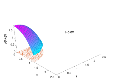
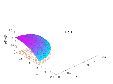
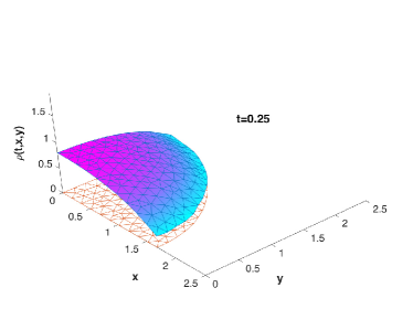
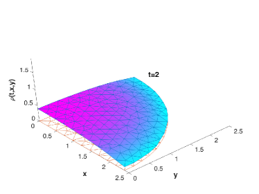
Figure 1. Numerical experiment 1: fully discrete evolution of our approximation for the self-similar solution to the free porous medium equation. Snapshots are taken at times $t=0.02$, $t=0.1$, $t=0.25$, and $t=2.0$.

For illustration, we present some numerical experiments from [CDMM18] for (30) with a cubic porous-medium nonlinearity $\Phi(r)=r^{3}$ and $V=0$. It is well-known (see, e.g., Vazquez [Váz07]) that in the long-time limit $t\to\infty$, arbitrary solutions approach a self-similar solution called the Barenblatt profile. To reduce numerical effort, we imposed a four-fold symmetry of the approximation: we use the quarter circle as computational domain $K$, and interprete the discrete function thereon as one of four symmetric pieces of the full discrete solution. To preserve reflection symmetry over time, homogeneous Neumann conditions are imposed on the artificial boundaries. This is implemented by reducing the degrees of freedom of the nodes along the $x$- and $y$-axes to tangential motion.

We initialize our simulation with a piecewise constant approximation of the Barenblatt profile at time $t=0.01$. We choose a time step $\tau=0.001$ and the final time $T=2$. In Figure 1, we have collected snapshots of the approximated density at different instances of time showing that the Barenblatt profile is well approximated. We refer for more details and other numerical tests to [CDMM18, Section 6].

4.2. Iteration of Lagrangian maps

We shall now review the ansatz made in [JMO17]. The basic idea is to put no a priori restrictions on $X:\Theta\to\Omega$ itself, but on its iterative updates. That is, we choose a finite dimensional set ${\mathcal{V}}$ of vector fields ${\mathbf{v}}:\Omega\to{\mathbb{R}}^{2}$ that are tangential to the boundary of $\Omega$, and “discretize” the variational problems (18) in space by minimizing only over Lagrangian maps of the form $X=(\operatorname{id}+{\Delta t}{\mathbf{v}})\circ X_{\Delta t}^{n-1}$, with ${\mathbf{v}}\in{\mathcal{V}}$. The two motivations for this ansatz are the following:

• If ${\mathcal{V}}$ only contains gradient vector fields, then the minimization problem (18) inherits the convexity of (15). Indeed, for ${\mathbf{v}}=\nabla\varphi$, one has

  $$\|(\operatorname{id}+{\Delta t}{\mathbf{v}})\circ X_{\Delta t}^{n-1}-X_{\Delta t}\|_{L^{2}_{\theta}} =\|(id+{\Delta t}{\mathbf{v}})-\operatorname{id}\|_{L^{2}_{(X_{\Delta t}^{n-1})\#\theta}}$$

  $$={\Delta t}{\mathbf{W}_{2}}\big{(}(\operatorname{id}+{\Delta t}{\mathbf{v}})\#(X_{\Delta t}^{n-1})\#\theta,(X_{\Delta t}^{n-1})\#\theta\big{)},$$

  which preserves the equivalence between (18) and (15).

• By choosing very regular ansatz functions in ${\mathcal{V}}$, one expects to otbain a higher order of consistency in space, at least for approximation of smooth solutions.

The particular choice made in [JMO17] are trigonometric polynomials,

$${\mathcal{V}}=\left\{{\mathbf{v}}=\nabla\varphi\,\middle|\,\varphi(x)=\sum_{k_{1},k_{2}=0}^{K}a_{k,\ell}\cos(\pi k_{1}x_{1})\cos(\pi k_{2}x_{2})\right\}.$$

The difficulty in the implementation of this scheme is that the Lagrangian map $X_{\Delta t}^{n}$ after the $n$th iteration is the concatenation of $n$ maps of the form $\operatorname{id}+{\Delta t}{\mathbf{v}}$, i.e.,

$$X_{\tau}^{n}=(\operatorname{id}+{\Delta t}{\mathbf{v}}_{\Delta t}^{n})\circ\cdots\circ(\operatorname{id}+{\Delta t}{\mathbf{v}}_{\Delta t}^{1})\circ X_{\tau}^{0}.$$

Naturally, these concatenations cannot be evaluated explicitly, and some further approximation needs to be performed for numerical approximation of the quantities in (18).

The ansatz made in [JMO17] is to distribute “test particles” $\xi_{m}$ in $\Omega$ and monitor their motion and evolution of density under the Lagragian map; these positions will be used as quadrature points for the integration in (18). Specifically, after the $n$ step, the position $x_{m}^{n}$ of $\xi_{m}$ and the density $\rho_{m}^{n}$ at $x_{m}^{n}$ are given by

$$x_{m}^{n}:=X_{\Delta t}^{n}(\xi_{m}),\quad\rho_{m}^{n}:=\frac{\rho_{m}^{0}}{\det\operatorname{D}X_{\Delta t}^{n}(\xi_{m})}.$$

Both quantities are easily obtained by iteration,

$$x_{m}^{n}=x_{m}^{n-1}+{\Delta t}{\mathbf{v}}^{n}(x_{m}^{n-1}),\quad\rho_{m}^{n}=\frac{\rho_{m}^{n-1}}{\det\big{(}{\mathbf{1}}+{\Delta t}\operatorname{D}{\mathbf{v}}_{\Delta t}^{n}(x_{m}^{n-1})\big{)}}$$

Finally, one assigns weights $\omega_{m}$ to the test particles, that can be understood as particle masses. The choice $\omega=1/M$ is obvious, however others improve the approximation quality of the integrals. In the numerical experiments in [JMO17], we have partitioned the domain $\Omega$ into $K\times K$ square cells, and have then used introduced equally distributed test particles with Lagrangian weights in each cell.

The iteration (18) now amounts to minimizing

(33) $$\sum_{m}\omega_{k}\left[\frac{{\Delta t}}{2}|{\mathbf{v}}(x^{n-1}_{k})|^{2}+h^{\#}\left(\frac{\rho_{m}^{n-1}}{\det\big{(}{\mathbf{1}}+{\Delta t}\operatorname{D}{\mathbf{v}}(x_{m}^{n-1})}\right)+V\big{(}x_{m}^{n-1}+{\Delta t}{\mathbf{v}}(x_{m}^{n-1})\big{)}\right].$$

The Euler Lagrange equations produce a a non-linear system of equations for the coefficients $a_{k,\ell}$ in ${\mathbf{v}}_{\Delta t}^{n}$.

The main results of [JMO17] are:

• The numerical scheme performs well in a variety of experiments.

• The functional (33) is uniformly convex of modulus $\frac{1}{{\Delta t}}+\lambda$ with respect to ${\mathbf{v}}\in{\mathcal{V}}$ (and thus strictly convex in terms of the coefficients $a_{k,\ell}$ for ${\Delta t}>0$ small enough).

• Assuming an a priori uniform bound on the density functions in $C^{5}(\Omega)$, one obtains convergence of the Lagrangian maps to a solution of (9).

4.3. Lagrangian maps from Laguerre cells

We briefly mention a semi-Lagrangian method developed in [BCMO16a] for numerical approximation of solutions to the Fokker-Planck equation (2). The scheme consists of two steps, that are carried out alternatingly: a Lagrangian one, in which a measure concentrated in $N$ points is transformed into a piecewise constant density function, and a projection step, in which the density function is again concentrated in $N$ point masses.

A central role is played by Laguerre cells, which we recall for convenience of the reader. Given $N$ points $\{x_{1},\ldots,x_{N}\}\in\Omega$ with respective real weights $\{\varphi_{1},\ldots,\varphi_{N}\}\in{\mathbb{R}}$, the corresponding $N$ Laguerre cells $\{L_{1},\ldots,L_{N}\}\subset\Omega$ are defined as follows: the $i$th cell $L_{i}$ consists of all $x\in\Omega$ such that $x\cdot x_{i}-\varphi_{i}\geq x\cdot x_{j}-\varphi_{j}$ for all $j$s. In the special case that the weights are $\varphi_{i}=\frac{1}{2}|x_{i}|^{2}$ for all $i$, the $L_{i}$ are precisely the Voronoi cells for the point configuration $x_{1},\ldots,x_{N}$. For general weights, the geometry of Laguerre cells can be much more complicated; for instance, one should not expect $x_{i}\in L_{i}$, and one can even have $L_{i}=\emptyset$ for one or several $i$’s. In any case, the $L_{1},\ldots,L_{N}$ cover $\Omega$ completely, and the intersection of two Laguerre cells is a convex set of lower dimension, possibly empty. In fact, it is obvious from the definition that $L_{i}\cap L_{j}$ lies in a hyperplane orthogonal to $x_{i}-x_{j}$. There is a characterization of Laguerre cells in terms of subdifferentials of convex functions. Namely, let $\varphi:\Omega\to{\mathbb{R}}$ be the largest convex function such that, on the one hand, $\varphi(x_{i})=\varphi_{i}$ at every $i$, and on the other hand, that $\nabla\varphi(\Omega)\subseteq\Omega$. This $\varphi$ is globally Lipschitz, and has corner singularities at each $x_{i}$. Recalling the definition of the subdifferential $\partial\varphi$, it is easily seen that $\partial\varphi(x_{i})=L_{i}$.

The ansatz for the Lagrangian step of the scheme in [BCMO16a] is to perform a minimizing movement, i.e. to solve the minimization problem (15) with $\mathcal{E}=\mathcal{H}_{h,0,0}$. The “old” measure $\rho_{\Delta t}^{n-1}$ is assumed to consist of $N$ Diracs at positions $\{x_{1},\ldots,x_{N}\}\in\Omega$ with respective masses $\{m_{1},\ldots,m_{N}\}$. The set of admissible $\rho$ in the minimization of (15) consists of absolutely continuous densities with the property that $\rho$ is piecewise constant on the $N$ Laguerre cells $\{L_{1},\ldots,L_{N}\}\subset\Omega$ for the given positions $\{x_{1},\ldots,x_{N}\}$ and some weights $\{\varphi_{1},\ldots,\varphi_{N}\}$, with the total mass in each $L_{i}$ equal to $m_{i}$. That is, the weights $\{\varphi_{1},\ldots,\varphi_{N}\}$ parametrize the space of admissible $\rho$’s. The subsequent projection step consists in determining some point in each $L_{i}$, e.g. the Steiner point, and concentrating the mass $m_{i}$ there.

There are several reasons for this choice of the Lagrangian step. One is that the Wasserstein distance from each admissible $\rho$ to the datum $\rho_{\Delta t}^{n-1}$ can be calculated explicitly. In fact, the aforementioned convex function $\varphi$ which extends the values of $\varphi_{i}$ at the $x_{i}$ is a Kantorovich potential for this transport. Another reason, which also makes this scheme very special, is that geodesic convexity of $\mathcal{H}_{h,0,0}$ is inherited under the discretization. More precisely, the map from the $N$-vector of values $\{\varphi_{1},\ldots,\varphi_{N}\}$ to the functional value $\mathcal{H}_{h,0,0}(\rho)$ at the respective piecewise constant density $\rho$ is convex.

In [BCMO16a], the ability of the numerical scheme is verified in a variety of experiments. On the analytical side, a rigorous proof is given for the $\Gamma$-convergence of the Lagrangian step to one step in the corresponding minimizing movement scheme in the limit of spatial refinement.

4.4. Particle approximation: blob method

Another Lagrangian approach to nonlinear aggregation-diffusion equations of the form (2) has been pursued in [CCP19b], also used in [CHWW19] for the Landau equation. The main strategy consists in using as approximation space for densities the set of finite linear combinations of Dirac Delta distributions. In other words, we want to approximate the gradient flow equations by a gradient flow in finite dimensions on the locations of these Dirac Deltas that we called particle locations. This approach is quite natural without diffusion $\Phi=0$. In fact, it is very much connected to the fact that the aggregation equation

(34) $$\partial_{t}\rho_{t}=\operatorname{div}\big{(}\rho_{t}\,[\nabla V+\rho_{t}\ast\nabla W]\big{)},$$

can be seen as the mean-field limit [CCH14, CDF⁺11, Jab14, CCHS19] of a particle system of the form

(35) $$\dot{x}_{i}=-\nabla V(x_{i})-\sum_{j\neq i}\nabla W(x_{i}-x_{j})m_{j}.$$

This can be formally understood by taking the ansatz

$$\rho_{t}\approx\rho^{N}_{t}=\sum_{i=1}^{N}\delta_{x_{i}(t)}m_{i},$$

where $\delta_{x_{i}}$ is a Dirac mass centered at $x_{i}\in\Omega$, into (34) as a distributional solution. The initialization is done by discretizing the initial datum $\rho_{0}$ as a finite sum of $N$ Dirac masses,

(36) $$\rho_{0}\approx\rho_{0}^{N}=\sum_{i=1}^{N}\delta_{x_{i}^{0}}m_{i},\qquad x_{i}^{0}\in\Omega,\quad m_{i}\geq 0.$$

The particle method (35) provides a semi-discrete numerical method preserving the gradient flow structure since the discrete energy $\mathcal{H}_{0,V,W}(\rho^{N}_{t})$ is decreased along the solutions of (35). In fact, the system (35) is a finite dimensional gradient flow of the discrete interaction energy $\mathcal{H}_{0,V,W}(\rho^{N}_{t})$ seen as a function of the particle locations.

The approach to generalize these deterministic particle methods for diffusive equations is not that obvious since we cannot evaluate the energy $\mathcal{H}_{h,0,0}(\rho)$ for finite linear combinations of Dirac Delta distributions. The main novelty introduced in [CCP19b] is to regularize the entropy functionals associated to diffusion equations. More precisely, let us take a mollifier $\varphi_{\epsilon}(x)=\varphi(x/\epsilon)/\epsilon^{d}$, $\epsilon>0$ for a given $\varphi$ smooth positive fast decaying function integrating to unity, i.e., we choose an approximation of the Dirac Delta at the origin. To showcase the regularization we propose, let us consider the particular case of the porous medium equation. Then, we propose to approximate the energy functional by

$$\mathcal{H}_{m}(\rho)=\int_{\Omega}\rho^{m}\,dx\approx\mathcal{H}_{m}^{\epsilon}(\rho)=\int_{\Omega}(\varphi_{\epsilon}*\rho)^{m-1}\rho\,dx.$$

The advantage of the approximated energy $\mathcal{H}_{m}^{\epsilon}(\rho)$ is that it makes sense for finite linear combination of Dirac Deltas. Other regularizations of the functional are possible, we chose this one since it leads to a pure particle system avoiding any continuous convolution as seen below.

The ultimate objective is then to approximate the gradient flow of the energy $\mathcal{H}_{m}(\rho)$ by the gradient flow of the regularized energy $\mathcal{H}_{m}^{\epsilon}(\rho)$. Finally, the regularized gradient flow can be approximated by the particle method in the same spirit as done earlier for the pure aggregation equation (34). Note that the case $m=2$ is special since we approximate the porous medium equation with $m=2$ by the aggregation equation with a repulsive smooth potential.

In general, giving the energy functional $\mathcal{H}_{h,V,W}(\rho)$ and assuming that $\Phi(r)=rF(r)$, we define the regularized functional as

(37) $${\mathcal{F}}_{\epsilon}(\rho)=\int_{\Omega}F(\varphi_{\epsilon}*\rho)\rho\,dx,$$

and

(38) $${\mathcal{E}}_{\epsilon}(\rho)=\int_{\Omega}F(\varphi_{\epsilon}*\rho)\rho\,dx+\int_{\Omega}\big{[}\rho V+\frac{1}{2}\rho(W\ast\rho)\big{]}\,\mathrm{d}x.$$

The gradient flow associated to this functional leads to $\partial_{t}\rho_{t}=\operatorname{div}\big{(}\rho_{t}\nabla\frac{\delta{\mathcal{E}}_{\epsilon}}{\delta\rho}\big{)}$ with the variations given at any density $\rho$ of ${\mathcal{F}}_{\epsilon}$ given by

$$\frac{\delta\mathcal{F}_{\epsilon}}{\delta\rho}(\rho)=\varphi_{\epsilon}*(F^{\prime}\circ(\varphi_{\epsilon}*\rho)\rho)+F\circ(\varphi_{\epsilon}*\rho).$$

Then $\rho^{N}_{t}$ satisfies the weak formulation $\partial_{t}\rho_{t}=\operatorname{div}\big{(}\rho_{t}\nabla\frac{\delta{\mathcal{F}}_{\epsilon}}{\delta\rho}\big{)}$ if and only if the particles follow the system

(39) $$\begin{cases}\displaystyle\dot{x}_{i}(t)=-\nabla V(x_{i}(t))-\sum_{j\neq i}\nabla W(x_{i}(t)-x_{j}(t))m_{j}-\nabla\frac{\delta{\mathcal{F}}_{\epsilon}}{\delta\rho}\left(\sum_{j}\delta_{x_{j}(t)}m_{j}\right)(x_{i}(t)),\\ x_{i}(0)=x_{i}^{0},\end{cases}$$

for $t\in[0,T]$. It is proven in [CCP19b, Corollary 5.5] that the ODE system (39) is well posed under suitable convexity and growth conditions of the potentials in case of working in the whole space for the power nonlinear diffusion $F(r)=r^{m}$ and $m\geq 2$. Moreover, the particle method was shown to be convergent to the solutions of (2) under suitable conditions, see [CCP19b, Theorem 5.6]. Notice that the right hand side of (39) can be expanded as

$$\nabla\frac{\delta{\mathcal{F}}_{\epsilon}}{\delta\rho}=\nabla\varphi_{\epsilon}*(F^{\prime}\circ\varphi_{\epsilon}*\rho)\rho)+F^{\prime}\circ(\varphi_{\epsilon}*\rho)(\nabla\varphi_{\epsilon}*\rho),$$

and that its evaluation in $\rho_{t}^{N}$ leads to the elimination of all convolutions by finite sums. In particular for linear diffusion leads to

$$\nabla\frac{\delta{\mathcal{F}}_{\epsilon}}{\delta\rho}=\nabla\varphi_{\epsilon}*\left(\frac{\rho}{\varphi_{\epsilon}*\rho}\right)+\frac{\nabla\varphi_{\epsilon}*\rho}{\varphi_{\epsilon}*\rho}.$$

Let us remark that the system (39) is a finite dimensional gradient flow in ${\mathbb{R}}^{dN}$ of the discrete regularized entropy functional ${\mathcal{E}}_{\epsilon}(\rho^{N})$ seen as a function of the particle positions $\{x_{1},\ldots,x_{N}\}\in{\mathbb{R}}^{d}$. Therefore, the system (39) keeps the gradient flow structure at the semidiscrete level and the discrete regularized energy is dissipated according to the same law of the continuous problem given by

$$\frac{d}{dt}{\mathcal{E}}_{\epsilon}(\rho^{N}(t))=-\int_{\Omega}\left|\nabla\frac{\delta{\mathcal{F}}_{\epsilon}}{\delta\rho}(\rho^{N}(t))\right|^{2}\rho^{N}(t)\,dx.$$

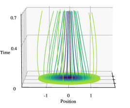
Figure 2. Two-Dimensional Keller–Segel Equation: Blowup with Supercritical Mass $9\pi$. Evolution of particle trajectories, colored according to the relative mass of each trajectory.

We illustrate the particle method (39) with some examples extracted from [CCP19b, Section 6] in which the mollifier is chosen as a Gaussian. We consider the classical Keller–Segel equation ($V=0$, $W(x)=1/(2\pi)\log|x|$, $m=1$) in two dimensions without normalizing the mass of the density. There is a dichotomy between global existence and blow-up given by the critical mass $8\pi$, and in particular, for supercritical initial data, solutions blow up in finite time [DP04, BDP06]. In Figure 2, we show the particles for the case of supercritical mass $9\pi$. Indeed, one of the benefits of our blob method approach is that the numerical method naturally extends to two and more dimensions, and we observe similar numerical performance independent of the dimension. We also plot the evolution of particle trajectories, observing the tendency of trajectories in regions of larger mass to be driven largely by pairwise attraction, while trajectories in regions of lower mass feel more strongly the effects of diffusion.

In Figures 3 and 2, the initial data is given by a Gaussian mollifier scaled to have mass that is either supercritical ($>8\pi$), critical ($=8\pi$), or subcritical ($<8\pi$) with respect to blowup behavior [DP04, BDP06]. In Figure 2, we observe how the particles associated to initial data with supercritical mass aggregate at the origin.

Two-Dimensional Keller–Segel Equation: Evolution of Density

t = 0.0                           t = 0.15    

Subcritical Mass $=7\pi$

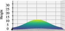
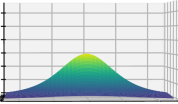
Critical Mass $=8\pi$

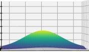
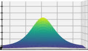
Supercritical Mass $=9\pi$

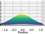
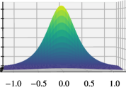
Figure 3. Evolution of numerical solutions for the two-dimensional Keller–Segel equation with subcritical, critical, and supercritical initial data.

4.5. Particle approximation: Yosida regularization

We briefly comment on a recent article [MLM⁺19], where the same idea as in [CCP19b] is pursued, but with a different regularization procedure. Again, a particle scheme for solution of the Fokker-Planck equation (2) is constructed, such that the empirical measure $\rho^{N}_{t}$ associated to $N$ moving particles in ${\mathbb{R}}^{d}$ approximates the the solution $\rho_{t}$ in the weak-$\star$ sense for measures. Here the $N$ particle positions $\{x_{1},\ldots,x_{N}\}\in{\mathbb{R}}^{d}$ obey an ODE system determined by the gradient flow on ${\mathbb{R}}^{dN}$ of a functional $\mathcal{H}^{\epsilon}$, similarly to (but less explicit than in) equations (39). We remark that [MLM⁺19] focuses on the linear Fokker-Planck equation with $W\equiv 0$ as well as on a model for crowd motion, but the basic idea directly generalizes to non-linear Fokker-Planck equations.

As discussed above, one cannot directly evaluate the energy $\mathcal{H}_{h,V,W}$ on the empirical measure $\rho^{N}$. Instead of “smearing out” the particles with a mollifier as in (37), the Yosida approximation of the internal energy is used, i.e.,

$$\mathcal{H}_{h,V,W}^{\epsilon}(\rho)=\inf_{\sigma}\left[\frac{1}{2\epsilon}{\mathbf{W}_{2}}(\rho,\sigma)^{2}+\int_{\Omega}h(\sigma)\,dx\right]+\int_{\Omega}\big{[}\rho V+\frac{1}{2}\rho(W\ast\rho)\big{]}\,dx,$$

For $\rho=\rho^{N}$ the empirical measure of $N$ particles, the second integral reduces to a finite sum. The Yosida approximation cannot be calculated explicitly (which is in contrast to the procedure in [CCP19b] explained above), but efficient methods for its numerical approximation have been developed recently in the context of semi-discrete optimal transport [KMT19]. The core idea is to obtain the Kantorovich potential $\psi$, which only needs to be defined at the $N$ particle positions $x_{1},\ldots,x_{N}$, by adjusting the corresponding Laguerre cells such that they satisfy a certain geometric condition.

Unconditional convergence of the empirical measures $\rho^{N}_{t}$ to the solution $\rho_{t}$ of (2) in the joint limit $N\to\infty$ and $\epsilon\to 0$ has been proven in dimension $d=1$. In higher space dimension, convergence can be shown if a certain uniform a priori bound is satisfied. Convexity of the regularized functional is not discussed; instead, it is shown that $\mathcal{H}_{h,V,W}^{\epsilon}(\rho^{N})$ is always semi-concave as a function on ${\mathbb{R}}^{Nd}$, which implies differentiability at all particle configurations with $N$ distinct point. After discretization in time by the implicit Euler method, a fully practical numerical scheme is obtained.

5. Optimize then discretize

We conclude by adopting the reverse strategy, that is first optimize then discretize. This idea was first proposed in [CM10] and further developed in [CRW16]. Both methods are based on different temporal and spatial discretizations of the optimality system to the respective $L^{2}$ gradient flow structure. This approach is particularly interesting in higher space dimension, where the calculation of the Wasserstein distance is computationally too expensive. The optimality system of (19) corresponds to a highly non-linear parabolic PDE for the diffeomorphism $X$. We will focus on the most general computational approach in the following; that is an implicit in time and finite element discretization in 2D, since all other schemes correspond to straight-forward simplifications.

We start from the optimality system of the $L^{2}$ gradient flow (18) with the transformed relative entropy (19). Then the diffeomorphism $X$ satisfies the following nonlinear PDE system in the limit $\Delta t\rightarrow 0$:

(40) $$\partial_{t}X =\operatorname{div}\left[\Psi^{\prime}(\det DX)(\operatorname{cof}DX)^{T}\right]-\nabla V\circ X-\int_{\Theta}\nabla W(X(\xi)-X(\xi^{\prime}))d\xi^{\prime},$$

We recall that the diffeomorphism $X$ corresponds to the map from a general reference measure to the unknown probability density $\rho_{t}$. We will consider the simplest case - that is the uniform density as a reference measure on $[0,1]^{2}$ - in the following. Then $\rho_{t}$ can be computed for sufficiently smooth $X$ via (21):

(41) $$\rho(X(\xi))\det(DX(\xi))=1.$$

5.1. Numerical scheme: multiD and finite element approach

We start by stating the semi-discrete implicit discretisation, where $\Delta t$ denotes the discrete time step, $t^{n+1}=(n+1)\Delta t$ and that $X^{n+1}$ corresponds to the solution $X=X(\xi,t)$ at time $t^{n+1}$. Then (40) reads as

(42) $$\begin{split}\frac{X^{n+1}-X^{n}}{\Delta t}=\,&\operatorname{div}[\Psi^{\prime}(\det DX^{n+1})(\operatorname{cof}DX^{n+1})]\\ &-\nabla V(X^{n+1})-\int_{\Theta}\nabla W(X^{n+1}(\xi)-X^{n+1}(\xi^{\prime}))d\xi.\end{split}$$

Its variational formulation for test functions $\varphi=\varphi(\xi)\in H^{1}(\Theta)$ defines a nonlinear operator $F$, which is given by:

(43) $$\begin{split}F(X,&\varphi)=\frac{1}{\Delta t}\int_{\Theta}(X^{n+1}-X^{n})\varphi(\xi)d\xi+\int_{\Theta}\Psi^{\prime}(\det DX^{n+1})(\operatorname{cof}DX^{n+1})\nabla\varphi(\xi)d\xi\\ +&\int_{\Theta}\nabla V(X^{n+1})\varphi(\xi)d\xi+\int_{\Theta}\left[\int_{\Theta}\nabla W(X^{n+1}(\xi)-X^{n+1}(\xi^{\prime}))d\xi^{\prime}\right]\varphi(\xi)d\xi.\end{split}$$

Then the fully discrete formulation can be obtained by choosing a suitable spatial discretisation. We choose lowest order $H^{1}$ conforming finite elements, that is elementwise linear functions, for $X$ as in (31). Note that we will use the same notation for the infinite dimensional and finite dimensional testfunctions to enhance reability in the following. The spatial discretisation defines the nonlinear operator equation $F(X,\varphi)=0$, which can be solved using Newton-Raphson’s method. In doing so, we compute the Jacobian matrix $DF$ of (43) as well as the $(k+1)$-th Newton update $Y^{n+1,k+1}$ via

(44) $$DF(X^{n+1,k},\varphi)Y^{n+1,k+1}=-F(X^{n+1,k},\varphi),$$

for all test functions $\varphi(\xi)\in H^{1}(\Theta)$. Note that the Jacobian matrix $DF$ is a full matrix and has no sparse structure due to the convolution operator $W$.
This discretisation can be used for a very general class of equations. Solutions to these equations often exhibit complex features, such as compact supports or concentration phenomena. This corresponds to diffeomorphisms $X_{t}$ becoming degenerate, and it is therefore often useful to perform a damped Newton update via:

$$X^{n+1,k+1}=X^{n+1,k}+\alpha Y^{n+1,k+1},$$

where $0<\alpha<1$ is a suitably chosen damping parameter. The Newton iteration (44) is terminated when a stopping criterion

$$\lvert F(X^{n+1,k+1},\varphi)\rvert\leq\epsilon_{1}\text{ or }\lVert X^{n+1,k+1}-X^{n+1,k}\rVert\leq\epsilon_{2},$$

for given error bounds $\epsilon_{1}>0$ and $\epsilon_{2}>0$ is satisfied. While the implicit in time discretization involves the solution of a nonlinear PDE system, it does not impose any CFL type condition on the time step as in the explicit case, see [CM10].

The ’optimise-than-discretise’ approach requires the transformation of the no-flux boundary conditions (4) as well as the computation of the initial diffeomorphism $X_{0}$ given $\rho_{0}$. The is not straight forward in higher space dimension and we will discuss the main ideas in $2D$ in the following.

Boundary conditions:

To formulate the respective no-flux boundary conditions for $X_{t}$ we consider diffeomorphisms, which map the boundary of the reference domain $\partial\Theta$ onto $\partial\Omega$ without rotations only. Then the translated no-flux boundary conditions (4) are given by

(45) $${\boldsymbol{\nu}}^{T}(\operatorname{cof}DX)^{T}\partial_{t}X=(\operatorname{cof}DX){\boldsymbol{\nu}}\cdot\partial_{t}X=0.$$

Note that (45) implies different conditions for different computational domains. Consider for example a rectangular mesh on $\Theta=[0,1]^{2}$ and $\Omega=[0,1]^{2}$. Then careful calculations yield

$$\partial_{\xi_{1}}X_{2}=0\text{ for }\xi_{1}=0,\xi_{1}=1\text{ and }\partial_{\xi_{2}}X_{1}=0\text{ for }\xi_{2}=0,\xi_{2}=1.$$

In case of a circles of radius $R$ equation (45) translates to

(46) $$\sin\theta\partial_{t}X_{2}\partial_{\xi_{1}}X_{1}+\cos\theta\partial_{t}X_{1}\partial_{\xi_{2}}X_{2} =0,$$

which implies

(47) $$X_{1}(\xi,t)=X_{2}(\xi,t)=\text{Id}.$$

This yields $\partial_{t}X_{1}=\partial_{t}X_{2}=0$ on the boundary.

Pre-processing and post-processing: calculating the initial diffeomorphism and the final density

We start by discussing how the initial diffeomorphism $X_{0}$ can be calculated given an initial density $\rho_{0}$. Different approaches have been proposed in the literature - depending on the spatial discretization of the underlying domain. We will review two possible constructions - the first is based on a splitting approach in case of rectangular meshes, while the second uses density equalising maps for triangular meshes.

Rectangular mesh:

This approach is based on splitting the problem in the $\xi_{1}$ and $\xi_{2}$ direction and solving the respective Monge-Kantorovich problems in each direction. This gives the following one-dimensional Monge-Kantorovich problem in the $\xi_{1}$ direction: determine $a_{i}$ at every mesh point $\xi_{1,i}\in[0,1)$ such that

$$\int_{0}^{a_{i}}\int_{0}^{1}\rho_{0}(\eta,\zeta)d\zeta d\eta=\xi_{1,i}.$$

Next we solve the Monge-Kantorovich problem in the $\xi_{2}$ direction. Hence we have to find $b_{ij}$ (which corresponds to the discrete value of a function $b$ at a grid point $\xi_{ij}=(i\Delta x,j\Delta y)$) such that

$$\int_{0}^{b_{ij}}\rho_{0}(a_{i},\eta)d\eta=\frac{\xi_{2}}{\sqrt{M}}\int_{0}^{1}\rho_{0}(a_{i},\eta)d\eta.$$

The initial diffeomorphism is then given by $X_{0}(\xi_{ij})=(a_{i},b_{ij})$.

Quadrilateral or triangular mesh:

In the case of general quadrilateral and triangular meshes the above construction does not work. Then one can solve the corresponding Monge Ampere equation (giving the optimal transportation plan in case of quadratic cost), use Knote theory or use density equalizing maps instead. We shall outline the latter approach, which is based on [Mos65], further studied in [ASMV03] and also used in cartography [GN04]. Hereby the initial diffeomorphism is constructed by following the heat flow, which transports an initial density to the uniform density, backwards in time. This approach is very flexible, since it can be used for general domains and only requires a fast heat equation solver.
Consider the heat equation on a bounded domain $\Omega\subset\mathbb{R}^{2}$ and solve

(48) $$\partial_{t}\rho+\operatorname{div}(\rho w)=0,\qquad\mbox{with }w=-\frac{\nabla\rho}{\rho},$$

with initial datum $\rho(0,x)=\rho_{0}(x)$ and homogeneous Neumann boundary conditions. The heat equation then transports the initial datum $\rho_{0}$ via the velocity field $w=-\frac{\nabla\rho}{\rho}$ towards its equilibration density $\bar{w}=\frac{1}{\lvert\Omega\rvert}\int_{\Omega}\rho_{0}(\xi)d\xi$ as $t\rightarrow\infty$. Then the cumulative displacement $\mathbf{x}(t)$ of any point at time $t$ is determined by integrating the velocity field, which corresponds to solving

$$\mathbf{x}(t)=\mathbf{x}(0)+\int_{0}^{t}w(t^{\prime},\mathbf{x}(t^{\prime}))\,dt^{\prime}.$$

As $t\rightarrow\infty$, the set of such displacements for all points $x=x(t)$ in $\Omega$, that is the grid points of the computational mesh, defines the new density-equalized domain. Note that we actually have to compute its inverse, since we need to find the map which maps the constant density to the initial density $\rho_{0}$.

Post-processing:

To obtain the final density $\rho_{T}:=\rho(\xi,t=T)$ from the final diffeomorphism $X_{T}:=X(\xi,t=T)$ we solve a regularized version of (41) (in 2D) given by:

(49) $$\varepsilon\Delta\rho_{T}(X_{T}(\xi))+\rho_{T}(X_{T}(\xi))=\frac{1}{\det DX_{T}(\xi)}\text{ with }0<\varepsilon\ll 1.$$

This can be accomplised by solving for example the respective variational formulation using finite elements. Note that the regularisation $\varepsilon\Delta\rho$ ensures a stable reconstruction in case of compactly supported or aggregated solutions.

Simulations

We conclude by illustrating the dynamics with different examples in 1D and 2D. All results are based on the implicit in time discretization (42), the spatial discretisation uses finite differences 1D and finite elements in 2D.

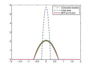
(a) Reconstructed BP profile $\rho=\rho(x,t)$ at time $t=0.021$.

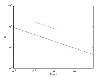
(b) Evolution of the entropy in time with a logarithmic scale for the y-axis.

Figure 4. Solution of the PME for $m=2$ after 2000 time steps.

In our first example we illustrate the behavior of our scheme for the porous medium equation (PME), which corresponds to $\Phi(s)=s^{m},m>1$ and $V=W=0$. The PME has self-similar solutions, the so-called Barenblatt Pattle profiles (BPP). We start our simulation with a BPP at time $t_{0}=10^{-3}$, i.e.

$$\rho_{0}(x)=\frac{1}{t_{0}^{\alpha}}\left(c-\alpha\frac{m-1}{2m}\frac{x^{2}}{t_{0}^{2\alpha}}\right)_{+}^{\frac{1}{m-1}},$$

where $\alpha=\frac{1}{m+1}$ and $c$ is chosen such that $\int_{-1}^{1}\rho_{0}(x)\,dx=2$. Figures 4 and 5 show the density profiles $\rho$ at time $t=0.021$ for $m=2$ and $m=4$. It also illustrates the evolution of the free energy in time, which decays like $t^{-\alpha(m-1)}$. As seen from Figures 4(b) and 5(b), these decays (indicated by the green lines) are perfectly captured by the scheme validating the chosen discretization.

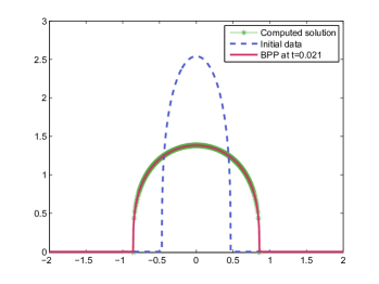
(a) Reconstructed BP profile $\rho=\rho(x,t)$ at time $t=0.021$.

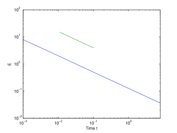
(b) Evolution of the entropy in time with a logarithmic scale for the y-axis.

Figure 5. Solution of the PME for $m=4$ after 2000 time steps.

Next we consider an agreggation equation with the logarithmic repulsive potential and harmonic confinement on the unit circle, that is $\Phi=0$ and

$$W(x)=\frac{\lvert x\rvert^{2}}{2}-\ln\lvert x\rvert$$

with an additional external potential of the form $V(x)=-\frac{\alpha}{\beta}\ln(\lvert x\rvert)$.

(a) Transformed mesh

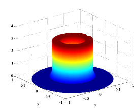
(b) Density $\rho$

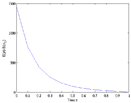
(c) Relative entropy

Figure 6. Simulation results for an attractive-repulsive potential $W=\frac{1}{2}\lvert x\rvert^{2}-\ln(\lvert x\rvert)$ and an additional potential $V=\frac{1}{4}\ln(\lvert x\rvert)$.

This model has been proposed as a way to find the spatial shape of the milling profiles in microscopic models for the dynamics of bird flocks. Figure 6 illustrates the corresponding annulus solution as well as the related computational challenges. The ’vacuum formation’ at the center distorts the mesh and leads to degeneracies in the diffeomorphism.

In our final example we consider the KS model with an initial Gaussian of mass one and $\chi=1.1\times 8\pi$. We observe the expected blow up in Figure 7. Figure 7(c) indicates that the free energy decay is changing concavity as the free energy tries to decay faster possibly tending to $-\infty$ at the blow-up time.

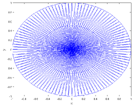
(a) Transformed mesh

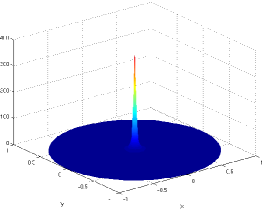
(b) Density $\rho$

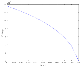
(c) Relative entropy

Figure 7. Simulation results for KS model with initial $M=1$ and $\chi=1.1\times 8\pi$.

5.2. 1D: Finite Difference approach

In this subsection, we briefly come back to the one dimensional problem as in the previous section and we show that certain finite differences method keep at the fully discrete level the asymptotic properties of the corresponding continuum problem. This general feature is quite desirable in general dimension for suitable approximations of the gradient flow equations (1). In fact, developing structure preserving schemes for general gradient flow equations is at the spotlight of research in this area, see [ABPP19, BCH18, CCP19a] for finite volume schemes or the particle schemes discussed in subsection 1.4.4-5 above. To showcase these methods developed in [GT06b, GT06a, BCC08, CM10] for certain particular nonlinear diffusion equations, we use the modified Keller-Segel model in one dimension corresponding to linear diffusion $h(\rho)=\rho\log\rho$ with interaction potential $W(x)=\frac{\chi}{\pi}\log|x|$ in selfsimilar variables, that is, in the presence of a quadratic external potential $V(x)=\frac{x^{2}}{2}$ as in [BCC08]. The Euler-Lagrange optimality conditions (42) can be rewritten in this particular case as

(50) $$-\frac{X^{n+1}(w)-X^{n}(w)}{\Delta t}=\frac{\partial}{\partial w}\left[\left(\frac{\partial X^{n+1}(w)}{\partial w}\right)^{-1}\right]+X^{n+1}(w)+\frac{\chi}{\pi}H[X^{n+1}]$$

where $H$ corresponds to the Hilbert transform defined by

$$H[X](w):=\frac{1}{\pi}\lim_{\epsilon\to 0}\int_{|X(w)-X(z)|\geq\epsilon}\frac{1}{X(w)-X(z)}\,\mathrm{d}z\,.$$

For sake of simplicity we assume that we have an equidistant mass distribution of size $\Delta m$. If we set $X^{n}_{i}:=X^{n}(i\Delta m)$, for any $i=0\cdots N$, and $N\Delta m=1$, the finite difference discretisation in space of (50) is the following implicit Euler scheme

(51) $$-\frac{X^{n+1}_{i}-X^{n}_{i}}{\Delta t}=\frac{1}{X^{n+1}_{i+1}-X^{n+1}_{i}}-\frac{1}{X^{n+1}_{i}-X^{n+1}_{i-1}}+X^{n+1}_{i}\\ +\frac{\chi}{\pi}\sum_{j\neq i|\geq\epsilon}\frac{\Delta m}{X^{n+1}_{i}-X^{n+1}_{j}}\;.$$

We impose Neumann boundary conditions, i.e. for any $n$, $\frac{1}{X^{n}_{N}-X^{n}_{N-1}}=0$ and $\frac{1}{X^{n}_{1}-X^{n}_{0}}=0$, so that the ’centre of mass’ is conserved. That is for all $n$

$$\sum_{i=0}^{N}X^{n}_{i}=0.$$

The solution at each time step of the non-linear system of equations is obtained by an iterative Newton-Raphson procedure as in the previous subsection. The motivation for this numerical scheme is that we are able to show that for a fixed $\Delta t>0$, the discrete solution converges to a unique steady state as time goes to infinity. To be precise the claim is the following: Assume $\chi<\chi_{c}$. Then the solution of the numerical scheme (51) converges to the (unique) steady-state of the problem at an exponential rate.

First we need the following two characterizations of the (unique) equilibrium state. The uniqueness will in fact follow from the convergence proof, as we shall see later. The discrete function $(U_{i})$ is an equilibrium if and only if for all $i$

(52) $$0=\frac{1}{U_{i+1}-U_{i}}-\frac{1}{U_{i}-U_{i-1}}+U_{i}+\frac{\chi}{\pi}\sum_{j\neq i}\frac{\Delta m}{U_{i}-U_{j}},$$

or equivalently for all $k$

(53) $$(U_{k+1}-U_{k})\left\{\frac{\chi}{\pi}\sum_{j=0}^{k}\sum_{i=k+1}^{N}\frac{\Delta m}{U_{i}-U_{j}}-\sum_{i=0}^{k}U_{i}\right\}=1.$$

To see that (52) and (53) are equivalent, rewrite the latter as

$$\forall k\quad\frac{1}{U_{k+1}-U_{k}}=\frac{\chi}{\pi}\sum_{j=0}^{k}\sum_{i=k+1}^{N}\frac{\Delta m}{U_{i}-U_{j}}-\sum_{i=0}^{k}U_{i},$$

and then ’derive’ it in a discrete way. Let us assume the existence of this equilibrium for $\chi<\chi_{c}$, easy to obtain by a discrete minimization argument. We proceed as computing the discrete time evolution of the $L^{2}-$distance between $X^{n}$ and the stationary state $U$, that is, the discrete counterpart of the 2-Wasserstein distance between $X^{n}$ and $U$ given by

$$\|X^{n}-U\|^{2}=\sum_{i}(X^{n+1}_{i}-U_{i})^{2}.$$

We deduce that

$$\frac{1}{2\Delta t}\Big{(}\|X^{n+1}-U\|^{2}\!-\|X^{n}-U\|^{2}\Big{)}\! =\!\frac{1}{2\Delta t}\sum_{i}(X^{n+1}_{i}-X^{n}_{i})(X^{n+1}_{i}+X^{n}_{i}-2U_{i})$$

$$\leq\sum_{i}\frac{X^{n+1}_{i}-X^{n}_{i}}{\Delta t}(X^{n+1}_{i}-U_{i}).$$

We then input the evolution equation for $X^{n+1}-X^{n}$, and obtain thanks to (52),

$$\frac{1}{2\Delta t}\Big{(}\|X^{n+1}-U\|^{2}-\|X^{n}-U\|^{2}\Big{)} \leq-\sum_{i}\Big{(}\frac{1}{X_{i+1}-X_{i}}-\frac{1}{X_{i}-X_{i-1}}-\frac{1}{U_{i+1}-U_{i}}$$

$$\quad\quad\quad+\frac{1}{U_{i}-U_{i-1}}+X_{i}-U_{i}+\frac{\chi}{\pi}\sum_{j\neq i}\frac{\Delta m}{X_{i}-X_{j}}$$

$$\quad\quad\quad-\frac{\chi}{\pi}\sum_{j\neq i}\frac{\Delta m}{U_{i}-U_{j}}\Big{)}(X_{i}-U_{i})$$

$$=A_{n}+B_{n}+C_{n},$$

where $V$ stands for $X^{n+1}$ without any ambiguity. We integrate by part the first (diffusion) contribution,

$$A =-\sum_{i}\Big{(}\frac{1}{X_{i+1}-X_{i}}-\frac{1}{X_{i}-X_{i-1}}-\frac{1}{U_{i+1}-U_{i}}+\frac{1}{U_{i}-U_{i-1}}\Big{)}(X_{i}-U_{i})$$

$$=\sum_{i}\Big{(}\frac{1}{X_{i+1}-X_{i}}-\frac{1}{U_{i+1}-U_{i}}\Big{)}(X_{i+1}-U_{i+1}-X_{i}+U_{i}).$$

We have carefully used the boundary conditions. We can rewrite $A$ using zero-homogeinity of the last expression, namely

$$A=\sum_{i}\gamma\Big{(}\frac{X_{i+1}-X_{i}}{U_{i+1}-U_{i}}\Big{)},$$

where $\gamma(\lambda)=2-\lambda-\lambda^{-1}$ is concave and non-positive. The second contribution coming from variables rescaling is obvious but crucial, namely

$$B=-\sum_{i}(X_{i}-U_{i})^{2}=-\|X^{n+1}-U\|^{2}.$$

The last (interaction) contribution is given by

$$C =-\frac{\chi}{\pi}\sum_{i}\Big{(}\sum_{j\neq i}\frac{\Delta m}{X_{i}-X_{j}}-\sum_{j\neq i}h\frac{\Delta m}{U_{i}-U_{j}}\Big{)}(X_{i}-U_{i})$$

$$=-\frac{\chi}{2\pi}\sum\sum_{i,j,\,i\neq j}{\Delta m}\Big{(}\frac{1}{X_{i}-X_{j}}-\frac{1}{U_{i}-U_{j}}\Big{)}(X_{i}-X_{j}-U_{i}+U_{j})$$

$$=-\frac{\chi}{2\pi}\sum\sum_{i,j,\,i\neq j}{\Delta m}\,\gamma\Big{(}\frac{X_{i}-X_{j}}{U_{i}-U_{j}}\Big{)}.$$

We refer to [BCC08] to check that the concavity of $\gamma$ shows that

$$C\leq-\sum_{k}\gamma\Big{(}\frac{V^{k+1}-V^{k}}{U^{k+1}-U^{k}}\Big{)}(U^{k+1}-U^{k})\left\{\frac{\chi}{\pi}\sum_{j=0}^{k}\sum_{i=k+1}^{N}\frac{\Delta m}{U_{i}-U_{j}}-\sum_{i=0}^{k}U_{i}\right\}.$$

The alternative representation of the stationary solution (53) implies that $A+C\leq 0$. As a consequence we obtain

(54) $$\frac{1}{2\Delta t}\Big{(}\|X^{n+1}-U\|^{2}-\|X^{n}-U\|^{2}\Big{)}\leq-\|X^{n+1}-U\|^{2}.$$

We finally get the exponential convergence rate,

$$\|X^{n}-U\|^{2}\leq\Big{(}\frac{1}{1+2\Delta t}\Big{)}^{n}\|X^{0}-U\|^{2}.$$

If $\Delta t$ is small, we can thus approximate $\log(1+2\Delta t)\approx 2\Delta t$ and $\Big{(}\frac{1}{1+2\Delta t}\Big{)}^{n}\approx\exp(-2n\Delta t)\approx\exp(-2t)$. Thus, the bound on the rate, we find, does not depend on the parameter $\chi<\chi_{c}$.

We can deduce a posteriori the uniqueness of the equilibrium. As a matter of fact let consider another equilibrium state $\tilde{U}$ and set $X^{n+1}=X^{n}=\tilde{U}$ in the above computations. We eventually obtain $\|\tilde{U}-U\|\leq 0$ from (54), which proves the uniqueness.

6. Other variational approaches

In this final section, we want to briefly mention another recent line of research for computing the solutions of the variational scheme (15) and even calculate the optimal transportation problem, i.e., computing the geodesic curve joining two given densities. This line of research deals with the following dynamic reformulation of the Wasserstein distance ${\mathbf{W}_{2}}(\rho_{0},\rho_{1})$ due to Benamou and Brenier [BB00], where the distance is obtained as

(55) $${\mathbf{W}_{2}}(\rho_{0},\rho_{1})=\inf_{(\rho,{\mathbf{v}})\in\mathcal{C}_{0}}\left\{\int_{0}^{1}\int_{\Omega}|{\mathbf{v}}(x,t)|^{2}\,\mathrm{d}\rho(x,t)\mathrm{d}t\right\}^{1/2},$$

where $(\rho,{\mathbf{v}})\in AC(0,1;{\mathcal{P}}(\Omega))\times L^{1}(0,1;L^{2}(\rho))$ belongs to the constraint set $\mathcal{C}_{0}$ provided that

(56) $$\partial_{t}\rho+\nabla\cdot(\rho{\mathbf{v}})=0 \,\,\text{ on }\Omega\times[0,1]$$

(57) $$(\rho{\mathbf{v}})\cdot{\boldsymbol{\nu}}=0 \,\,\text{ on }\partial\Omega\times[0,1],$$

(58) $$\rho(\cdot,0)=\rho_{0},\ \rho(\cdot,1)=\rho_{1} \,\,\text{ on }\Omega.$$

A curve $\rho$ in ${\mathcal{P}}(\Omega)$ is absolutely continuous in time, denoted $\rho\in AC(0,1;{\mathcal{P}}(\Omega))$, if there exists $w\in L^{1}(0,1)$ so that ${\mathbf{W}_{2}}(\rho(\cdot,t_{0}),\rho(\cdot,t_{1}))\leq\int_{t_{0}}^{t_{1}}w(s)\mathrm{d}s$ for all $0<t_{0}\leq t_{1}<1$. The PDE constraint (56-57) holds in the duality with smooth test functions on ${\mathbb{R}^{d}}\times[0,1]$, i.e. for all $f\in C^{\infty}_{c}({\mathbb{R}^{d}}\times[0,1])$,

$$\int_{0}^{1}\int_{\Omega}\left[\partial_{t}f(x,t)\rho(x,t)\right. +\left.\nabla f(x,t)\cdot{\mathbf{v}}(x,t)\rho(x,t)\right]\mathrm{d}x\mathrm{d}t$$

$$+\int_{\Omega}\left[f(x,0)\rho_{0}(x)-f(x,1)\rho_{1}(x)\right]\mathrm{d}x=0\,.$$

This dynamic reformulation reduces the problem of finding the Wasserstein distance between any two measures to identifying the curve in ${\mathcal{P}}(\Omega)$ that connects them with minimal kinetic energy. Since (55) is not strictly convex, and the PDE constraint (56) is nonlinear, in Benamou and Brenier’s original work, they restrict their attention to the case $\rho(\cdot,t)\in{\mathcal{P}}_{ac}(\Omega)$ and introduce the momentum variables $m={\mathbf{v}}\rho$, in order to rewrite (55) as

(59) $${\mathbf{W}_{2}}(\rho_{0},\rho_{1})^{2}=\min_{(\rho,m)\in\mathcal{C}_{1}}\int_{0}^{1}\int_{\Omega}\Phi(\rho(x,t),m(x,t))\mathrm{d}x\,\mathrm{d}t,$$

where

$$\Phi(\rho,m)=\begin{cases}\frac{\|m\|^{2}}{\rho}&\text{ if }\rho>0\\ 0&\text{ if }(\rho,m)=(0,0)\\ \infty&\text{ otherwise}\end{cases}$$

and $(\rho,m)\in AC(0,1;{\mathcal{P}}_{ac}(\Omega))\times L^{1}(0,1;L^{2}(\rho^{-1}))$ belong to the constraint set $\mathcal{C}_{1}$ provided that

$$\partial_{t}\rho+\nabla\cdot m=0 \,\,\text{ on }\Omega\times[0,1]$$

$$m\cdot{\boldsymbol{\nu}}=0 \,\,\text{ on }\partial\Omega\times[0,1].$$

$$\rho(\cdot,0)=\rho_{0},\ \rho(\cdot,1)=\rho_{1} \,\,\text{ on }\Omega.$$

After this reformulation, the integral functional

(60) $$(\rho,m)\mapsto\int_{0}^{1}\int_{\Omega}\Phi(\rho,m)$$

is strictly convex along linear interpolations and lower semicontinuous with respect to weak-* convergence [AFP00, Example 2.36], and the PDE constraint is linear. As an immediate consequence, one can conclude that minimizers are unique. Furthermore, for any $\rho_{0},\rho_{1}\in{\mathcal{P}}_{ac}(\Omega)$, a direct computation shows that the minimizer $(\bar{\rho},\bar{m})$ is given by the Wasserstein geodesic from $\rho_{0}$ to $\rho_{1}$, see [Vil03a, AGS05, San15] for further background on optimal transport. Furthermore, given any minimizer $(\bar{\rho},\bar{m})$ of (59), one can recover the optimal transport map in terms of $(\bar{\rho},\bar{v})$. Building upon Benamou and Brenier’s dynamic reformulation of the Wasserstein distance, one can also consider a dynamic reformulation of the JKO scheme (15). In particular, substituting (59) in (15) leads to the following dynamic JKO scheme: given $\Delta t>0$, $\mathcal{E}$, and $\rho_{0}$, solve the constrained optimization problem,

$$\inf_{(\rho,m)\in\mathcal{C}}\int_{0}^{1}\int_{\Omega}\Phi(\rho(x,t),m(x,t))\,\mathrm{d}x\mathrm{d}t+2\Delta t\mathcal{E}(\rho(\cdot,1)),$$

where $(\rho,m)\in AC(0,1;{\mathcal{P}}_{ac}(\Omega))\times L^{1}(0,1;L^{2}(\rho^{-1}))$ belong to the constraint set $\mathcal{C}$ provided that

(61) $$\partial_{t}\rho+\nabla\cdot m=0 \text{ on }\Omega\times[0,1],\,m\cdot\eta=0\text{ on }\partial\Omega\times[0,1],\,\text{ and }\rho(\cdot,0)=\rho_{0}\text{ on }\Omega.$$

This Eulerian approach to optimal transport has also been used for numerical purposes. In fact, the first numerical methods for the Wasserstein distance were done in this formulation in the seminal paper of Benamou and Brenier [BB00] by using the augmented Lagrangian method ALG2 for convex optimization problems. More recently, modern proximal splitting methods have been used by Papadakis, Peyre, and Oudet in [PPO14]. Adding an additional Fisher information term in this dynamic formulation (in analogy with entropic regularization) has also been explored in [LYOnt]. For a detailed survey of state of the art methods in computational optimal transport, we refer the reader to the recent book by Péyre and Cuturi in [PC18]. We also refer to the companion Chapter in this volume of Quentin Merigot.

However, this strategy has only been recently used for computing the Wasserstein distance integrated with the JKO scheme (15) in order to simulate partial differential equations of the form (1), see for instance [BCMO16b, BCL16, CCWW19, LLW19]. The approach in [CCWW19] is to discretize first the optimality conditions in (61) in order to solve numerically the corresponding optimization problem at the discrete level. The convexity of the problem at the discrete level is conserved as soon as the energy $\mathcal{E}$ is convex, since the functional related to the distance ${\mathbf{W}_{2}}$ is convex and the constraints are linear. Unlike [BCL16], which applied Benamou and Brenier’s classical ALG2 discretization to numerically approximate solutions of this minimization problem, the authors in [CCWW19] solve the optimization problem using a modern primal dual three operator splitting scheme due to Yan [Yan18]. The previous work by Papadakis, Peyre, and Oudet [PPO14] applied a similar two operator splitting scheme to simulate the Wasserstein distance. However, there are a few key differences in these two approaches. First, the implementation of the primal dual splitting scheme in [CCWW19] is done in a manner that does not require matrix inversion of the finite difference operator, which reduces the computational cost. In fact, the authors are able to obtain the exact expression for the proximal operator, which allows their method to be truly positivity preserving and very fast computationally.

Another key difference between these methods lies in the treatment of the linear PDE constraint in the dynamic reformulation of the Wasserstein distance. While most of previous work has imposed the linear PDE constraint exactly, via a finite difference approximation, the authors in [CCWW19] allow the linear PDE constraint to hold up to an error of order $\delta$, which can be tuned according to the spatial discretization $(\Delta x)$ and the inner temporal discretization $(\Delta t)$ to respect the order of accuracy of the finite difference approximation of the continuity equation and the error in the initial and boundary constraints. Numerically, this allows their method to converge in fewer iterations, without any reduction in accuracy. Theoretically, this allows them to prove convergence of minimizers of the fully discrete problem to minimizers of the JKO scheme (15), since minimizers of the fully discrete problem always exist, which is not the case when the PDE constraint is enforced exactly. Finally, let us mention that the authors in [LLW19] have explored the Fisher regularization of the optimal transportation cost leading to very good results and fast computational algorithms however, not solving exactly the JKO steps and therefore not being exactly energy decreasing at the fully discrete level. In summary, the Eulerian approach to solving the JKO minimization problem (15) is also being successfully and efficiently applied for numerical purposes due to the smart use of recent advances in numerical methods for optimization of convex functionals.

Appendix

Energy on Lagrangian maps. We here compute the variational derivative of the functional $\mathcal{E}^{\#}(X)$.

Lemma 1.

With $\mathcal{E}^{\#}(X)=\mathcal{E}(X\#\theta)$, we have at each diffeomorphism $\bar{X}:\Theta\to\Omega$:

(62) $$\frac{1}{\theta}\frac{\delta\mathcal{E}^{\#}}{\delta X}(\bar{X})=\nabla\frac{\delta\mathcal{E}}{\delta\rho}(\bar{X}\#\theta)\circ\bar{X}.$$

Proof.

Let ${\mathbf{v}}\in C^{\infty}_{c}(\Omega)$ be a smooth vector field, and define perturbations $(X^{s})_{s\in{\mathbb{R}}}$ of $\bar{X}$ via the flow of ${\mathbf{v}}$, that is

$$\partial_{s}X^{s}={\mathbf{v}}\circ X^{s},\quad X^{0}=\bar{X}.$$

On the one hand,

$$\frac{\mathrm{d}}{\,\mathrm{d}s}\bigg{|}_{s=0}\mathcal{E}^{\#}(X^{s})=\int_{\Theta}\frac{\delta\mathcal{E}^{\#}}{\delta X}(X^{s})\cdot\partial_{s}X^{s}\,\mathrm{d}\xi\bigg{|}_{s=0}=\int_{\Theta}\frac{\delta\mathcal{E}^{\#}}{\delta X}(\bar{X})\cdot{\mathbf{v}}\circ\bar{X}\,\mathrm{d}\xi.$$

And on the other hand, since

$$\partial_{s}(X^{s}\#\theta)=-\operatorname{div}\big{(}X^{s}\#\theta\,{\mathbf{v}})$$

by the properties of the push-forward, we have that

$$\frac{\mathrm{d}}{\,\mathrm{d}s}\bigg{|}_{s=0}\mathcal{E}(X^{s}\#\theta) =\int_{\Omega}\frac{\delta\mathcal{E}}{\delta\rho}(X^{s}\#\theta)\,\partial_{s}(X^{s}\#\theta)\,\mathrm{d}x\bigg{|}_{s=0}$$

$$=\int_{\Omega}\nabla\frac{\delta\mathcal{E}}{\delta\rho}(\bar{X}\#\theta)\cdot(\bar{X}\#\theta\,{\mathbf{v}})\,\mathrm{d}x$$

$$=\int_{\Theta}\left[\nabla\frac{\delta\mathcal{E}}{\delta\rho}(\bar{X}\#\theta)\right]\circ\bar{X}\cdot{\mathbf{v}}\circ\bar{X}\,\theta\,\mathrm{d}\xi.$$

Since ${\mathbf{v}}$ is arbitrary, and $\bar{X}$ is a diffeomorphism, the fact that $\mathcal{E}^{\#}(X^{s})$ and $\mathcal{E}(X^{s}\#\theta)$ — and hence also their $s$-derivatives — are equal implies (62). ∎

References

- [ABPP19] Luis Almeida, Federica Bubba, Benoît Perthame, and Camille Pouchol. Energy and implicit discretization of the Fokker-Planck and Keller-Segel type equations. Netw. Heterog. Media, 14(1):23–41, 2019.
- [AFP00] Luigi Ambrosio, Nicola Fusco, and Diego Pallara. Functions of bounded variation and free discontinuity problems, volume 254. Clarendon Press Oxford, 2000.
- [AGS05] L. Ambrosio, N. Gigli, and G. Savaré. Gradient flows. Springer, 2005.
- [AGS08] Luigi Ambrosio, Nicola Gigli, and Giuseppe Savaré. Gradient flows in metric spaces and in the space of probability measures. Lectures in Mathematics ETH Zürich. Birkhäuser Verlag, Basel, second edition, 2008.
- [ALS06] Luigi Ambrosio, Stefano Lisini, and Giuseppe Savaré. Stability of flows associated to gradient vector fields and convergence of iterated transport maps. Manuscripta Math., 121(1):1–50, 2006.
- [ASMV03] Albert Avinyo, Joan Sola-Morales, and Marta Valencia. On maps with given Jacobians involving the heat equation. Zeitschrift für angewandte Mathematik und Physik, 54(6):919–936, 2003.
- [BB00] J.-D. Benamou and Y. Brenier. A computational fluid mechanics solution to the Monge-Kantorovich mass transfer problem. Numer. Math., 84:375–393, 2000.
- [BCC08] Adrien Blanchet, Vincent Calvez, and José A. Carrillo. Convergence of the mass-transport steepest descent scheme for the subcritical Patlak-Keller-Segel model. SIAM J. Numer. Anal., 46(2):691–721, 2008.
- [BCC12] Adrien Blanchet, Eric A. Carlen, and José A. Carrillo. Functional inequalities, thick tails and asymptotics for the critical mass Patlak-Keller-Segel model. J. Funct. Anal., 262(5):2142–2230, 2012.
- [BCH18] Rafael Bailo, Jose A. Carrillo, and Jingwei Hu. Fully discrete positivity-preserving and energy-dissipating schemes for aggregation-diffusion equations with a gradient flow structure. to appear in Comm. Math. Sci., Preprint arXiv 1811.11502, 2018.
- [BCL09] Andrea L. Bertozzi, José A. Carrillo, and Thomas Laurent. Blow-up in multidimensional aggregation equations with mildly singular interaction kernels. Nonlinearity, 22(3):683–710, 2009.
- [BCL16] J.-D. Benamou, G. Carlier, and M. Laborde. An augmented Lagrangian approach to Wasserstein gradient flows and applications. ESAIM: PROCEEDINGS AND SURVEYS, 54:1–17, 2016.
- [BCLR13a] D. Balagué, J. A. Carrillo, T. Laurent, and G. Raoul. Dimensionality of local minimizers of the interaction energy. Arch. Ration. Mech. Anal., 209(3):1055–1088, 2013.
- [BCLR13b] D. Balagué, J. A. Carrillo, T. Laurent, and G. Raoul. Nonlocal interactions by repulsive-attractive potentials: radial ins/stability. Phys. D, 260:5–25, 2013.
- [BCMO16a] Jean-David Benamou, Guillaume Carlier, Quentin Mérigot, and Édouard Oudet. Discretization of functionals involving the Monge-Ampère operator. Numer. Math., 134(3):611–636, 2016.
- [BCMO16b] Jean-David Benamou, Guillaume Carlier, Quentin Mérigot, and Édouard Oudet. Discretization of functionals involving the Monge-Ampère operator. Numer. Math., 134(3):611–636, 2016.
- [BDP06] Adrien Blanchet, Jean Dolbeault, and Benoî t Perthame. Two-dimensional Keller–Segel model: optimal critical mass and qualitative properties of the solutions. Electron. J. Differential Equations, pages No. 44, 32, 2006.
- [Ber98] Andrea L Bertozzi. The mathematics of moving contact lines in thin liquid films. Notices of the AMS, 45(6):689–697, 1998.
- [BGL12] A. Bertozzi, J. Garnett, and T. Laurent. Characterization of radially symmetric finite time blowup in multidimensional aggregation equations. SIAM Journal on Mathematical Analysis, 44(2):651–681, 2012.
- [Bre91] Yann Brenier. Polar factorization and monotone rearrangement of vector-valued functions. Comm. Pure Appl. Math., 44(4):375–417, 1991.
- [CCH14] José Antonio Carrillo, Young-Pil Choi, and Maxime Hauray. The derivation of swarming models: mean-field limit and Wasserstein distances. In Collective Dynamics from Bacteria to Crowds: An Excursion Through Modeling, Analysis and Simulation, volume 553 of CISM Courses and Lect., pages 1–46. Springer Vienna, 2014.
- [CCHS19] José A. Carrillo, Young-Pil Choi, Maxime Hauray, and Samir Salem. Mean-field limit for collective behavior models with sharp sensitivity regions. J. Eur. Math. Soc. (JEMS), 21(1):121–161, 2019.
- [CCP19a] José A. Carrillo, Young-Pil Choi, and Lorenzo Pareschi. Structure preserving schemes for the continuum Kuramoto model: phase transitions. J. Comput. Phys., 376:365–389, 2019.
- [CCP19b] José Antonio Carrillo, Katy Craig, and Francesco S. Patacchini. A blob method for diffusion. Calc. Var. Partial Differential Equations, 58(2):Art. 53, 53, 2019.
- [CCWW19] Jose A. Carrillo, Katy Craig, Li Wang, and Chaozhen Wei. Primal dual methods for Wasserstein gradient flows, 2019.
- [CCY19] José A. Carrillo, Katy Craig, and Yao Yao. Aggregation-diffusion equations: dynamics, asymptotics, and singular limits. In Active particles, Vol. 2, Model. Simul. Sci. Eng. Technol., pages 65–108. Birkhäuser/Springer, Cham, 2019.
- [CDF+11] J. A. Carrillo, M. DiFrancesco, A. Figalli, T. Laurent, and D. Slepčev. Global-in-time weak measure solutions and finite-time aggregation for nonlocal interaction equations. Duke Math. J., 156(2):229–271, 2011.
- [CDMM18] José A. Carrillo, Bertram Düring, Daniel Matthes, and David S. McCormick. A Lagrangian scheme for the solution of nonlinear diffusion equations using moving simplex meshes. J. Sci. Comput., 75(3):1463–1499, 2018.
- [CHR20] José A. Carrillo, Katharina Hopf, and José L. Rodrigo. On the singularity formation and relaxation to equilibrium in 1D Fokker-Planck model with superlinear drift. Adv. Math., 360:106883, 66, 2020.
- [CHWW19] Jose A. Carrillo, Jingwei Hu, Li Wang, and Jeremy Wu. A particle method for the homogeneous Landau equation, 2019.
- [CL10] José Antonio Carrillo and Stefano Lisini. On the asymptotic behavior of the gradient flow of a polyconvex functional. In Nonlinear partial differential equations and hyperbolic wave phenomena, volume 526 of Contemp. Math., pages 37–51. Amer. Math. Soc., Providence, RI, 2010.
- [CM10] J. A. Carrillo and J. S. Moll. Numerical simulation of diffusive and aggregation phenomena in nonlinear continuity equations by evolving diffeomorphisms. SIAM J. Sci. Comput., 31(6):4305–4329, 2009/10.
- [CMV03] José A. Carrillo, Robert J. McCann, and Cédric Villani. Kinetic equilibration rates for granular media and related equations: entropy dissipation and mass transportation estimates. Rev. Mat. Iberoamericana, 19(3):971–1018, 2003.
- [CMV06] José A. Carrillo, Robert J. McCann, and Cédric Villani. Contractions in the 2-Wasserstein length space and thermalization of granular media. Arch. Ration. Mech. Anal., 179(2):217–263, 2006.
- [CN10] Fausto Cavalli and Giovanni Naldi. A Wasserstein approach to the numerical solution of the one-dimensional Cahn-Hilliard equation. Kinet. Relat. Models, 3(1):123–142, 2010.
- [CRW16] José A Carrillo, Helene Ranetbauer, and Marie-Therese Wolfram. Numerical simulation of nonlinear continuity equations by evolving diffeomorphisms. Journal of Computational Physics, 327:186–202, 2016.
- [CT04] Jose Antonio Carrillo and Giuseppe Toscani. Wasserstein metric and large–time asymptotics of nonlinear diffusion equations. In New Trends in Mathematical Physics: In Honour of the Salvatore Rionero 70th Birthday, pages 234–244. World Scientific, 2004.
- [DP04] Jean Dolbeault and Benoî t Perthame. Optimal critical mass in the two-dimensional Keller–Segel model in . C. R. Math. Acad. Sci. Paris, 339(9):611–616, 2004.
- [ESG05] L. C. Evans, O. Savin, and W. Gangbo. Diffeomorphisms and nonlinear heat flows. SIAM J. Math. Anal., 37(3):737–751, 2005.
- [GN04] Michael T Gastner and Mark EJ Newman. Diffusion-based method for producing density-equalizing maps. PNAS, 101(20):7499–7504, 2004.
- [GST09] Ugo Gianazza, Giuseppe Savaré, and Giuseppe Toscani. The Wasserstein gradient flow of the Fisher information and the quantum drift-diffusion equation. Arch. Ration. Mech. Anal., 194(1):133–220, 2009.
- [GT06a] Laurent Gosse and Giuseppe Toscani. Identification of asymptotic decay to self-similarity for one-dimensional filtration equations. SIAM J. Numer. Anal., 43(6):2590–2606, 2006.
- [GT06b] Laurent Gosse and Giuseppe Toscani. Lagrangian numerical approximations to one-dimensional convolution-diffusion equations. SIAM J. Sci. Comput., 28(4):1203–1227, 2006.
- [HB10] Y. Huang and A. Bertozzi. Self-similar blowup solutions to an aggregation equation in . SIAM Journal on Applied Mathematics, 70(7):2582–2603, 2010.
- [HP05] Darryl D. Holm and Vakhtang Putkaradze. Aggregation of finite-size particles with variable mobility. Phys. Rev. Lett., 95:226106, Nov 2005.
- [Jab14] Pierre-Emmanuel Jabin. A review of the mean field limits for Vlasov equations. Kinet. Relat. Models, 7(4):661–711, 2014.
- [JKO98] Richard Jordan, David Kinderlehrer, and Felix Otto. The variational formulation of the Fokker-Planck equation. SIAM J. Math. Anal., 29(1):1–17, 1998.
- [JMO17] Oliver Junge, Daniel Matthes, and Horst Osberger. A fully discrete variational scheme for solving nonlinear Fokker-Planck equations in multiple space dimensions. SIAM J. Numer. Anal., 55(1):419–443, 2017.
- [Jün09] Ansgar Jüngel. Transport equations for semiconductors, volume 773. Springer, 2009.
- [KMT19] Jun Kitagawa, Quentin Mérigot, and Boris Thibert. Convergence of a newton algorithm for semi-discrete optimal transport. Journal of the European Mathematical Society, 21(9):2603–2651, Apr 2019.
- [LLW19] Wuchen Li, Jianfeng Lu, and Li Wang. Fisher information regularization schemes for Wasserstein gradient flows, 2019.
- [LT04] Hailiang Li and Giuseppe Toscani. Long-time asymptotics of kinetic models of granular flows. Archive for Rational Mechanics and Analysis, 172(3):407–428, May 2004.
- [LT17] Guillaume Legendre and Gabriel Turinici. Second-order in time schemes for gradient flows in Wasserstein and geodesic metric spaces. C. R. Math. Acad. Sci. Paris, 355(3):345–353, 2017.
- [LYOnt] W. Li, P. Ying, and S. Osher. Computations of optimal transport distance with fisher information regularizationn. arXiv:1704.04605, preprint.
- [McC97] Robert J. McCann. A convexity principle for interacting gases. Adv. Math., 128(1):153–179, 1997.
- [MLM+19] Quentin Merigot, Hugo Leclerc, Quentin Mérigot, Filippo Santambrogio, and Federico Stra. Lagrangian discretization of crowd motion and linear diffusion, 2019.
- [MMS09] Daniel Matthes, Robert J. McCann, and Giuseppe Savaré. A family of nonlinear fourth order equations of gradient flow type. Comm. Partial Differential Equations, 34(10-12):1352–1397, 2009.
- [MO14] Daniel Matthes and Horst Osberger. Convergence of a variational Lagrangian scheme for a nonlinear drift diffusion equation. ESAIM Math. Model. Numer. Anal., 48(3):697–726, 2014.
- [MO17] Daniel Matthes and Horst Osberger. A convergent Lagrangian discretization for a nonlinear fourth-order equation. Found. Comput. Math., 17(1):73–126, 2017.
- [Mos65] Jürgen Moser. On the volume elements on a manifold. Transactions of the American Mathematical Society, pages 286–294, 1965.
- [MP19] Daniel Matthes and Simon Plazotta. A variational formulation of the BDF2 method for metric gradient flows. ESAIM Math. Model. Numer. Anal., 53(1):145–172, 2019.
- [MS17] Daniel Matthes and Benjamin Söllner. Convergent Lagrangian discretization for drift-diffusion with nonlocal aggregation. In Innovative algorithms and analysis, volume 16 of Springer INdAM Ser., pages 313–351. Springer, Cham, 2017.
- [OM17] Horst Osberger and Daniel Matthes. Convergence of a fully discrete variational scheme for a thin-film equation. In Topological optimization and optimal transport, volume 17 of Radon Ser. Comput. Appl. Math., pages 356–399. De Gruyter, Berlin, 2017.
- [Osb15] Horst Osberger. Fully variational Lagrangian discretizations for second and fourth order evolution equations. Dissertation, Technische Universität München, München, 2015.
- [Osb17] Horst Osberger. Long-time behavior of a fully discrete Lagrangian scheme for a family of fourth order equations. Discrete Contin. Dyn. Syst., 37(1):405–434, 2017.
- [Ott98] Felix Otto. Lubrication approximation with prescribed nonzero contact angle. Comm. Partial Differential Equations, 23(11-12):2077–2164, 1998.
- [Ott01a] Felix Otto. The geometry of dissipative evolution equations: the porous medium equation. Comm. Partial Differential Equations, 26(1-2):101–174, 2001.
- [Ott01b] Felix Otto. The geometry of dissipative evolution equations: the porous medium equation. Comm. Partial Differential Equations, 26(1-2):101–174, 2001.
- [PC18] Gabriel Peyré and Marco Cuturi. Computational Optimal Transport. book in preparation, personal communication, 2018.
- [Pla19] Simon Plazotta. A BDF2-approach for the non-linear Fokker-Planck equation. Discrete Contin. Dyn. Syst., 39(5):2893–2913, 2019.
- [PPO14] N. Papadakis, G. Peyre, and E. Oudet. Optimal transport with proximal splitting. SIAM. J. Image. Sci., 7(1):212–238, 2014.
- [San15] Filippo Santambrogio. Optimal transport for applied mathematicians. Birkäuser, NY, pages 99–102, 2015.
- [Tos00] Giuseppe Toscani. One-dimensional kinetic models of granular flows. M2AN Math. Model. Numer. Anal., 34(6):1277–1291, 2000.
- [Váz07] Juan Luis Vázquez. The porous medium equation: mathematical theory. Oxford University Press, 2007.
- [Vil03a] C. Villani. Topics in Optimal Transport. 58 AMS. Grad. Stud. Math., 2003. Providence, RI.
- [Vil03b] Cédric Villani. Topics in Optimal Transportation, volume 58 of Graduate Studies in Mathematics. American Mathematical Society, Providence, RI, 2003.
- [WW10] Michael Westdickenberg and Jon Wilkening. Variational particle schemes for the porous medium equation and for the system of isentropic Euler equations. M2AN Math. Model. Numer. Anal., 44(1):133–166, 2010.
- [Yan18] Ming Yan. A new primal–dual algorithm for minimizing the sum of three functions with a linear operator. Journal of Scientific Computing, pages 1–20, 2018.