Single spin asymmetry $A_{UL}^{\sin(\phi_{h}-\phi_{R})}$ in dihadron semi-inclusive DIS

Abstract

In this paper we study the single longitudinal spin asymmetry $A_{UL}^{\sin(\phi_{h}-\phi_{R})}$ of dihadron production in semi-inclusive deep inelastic scattering (SIDIS) via helicity-dependent dihadron fragmentation function (DiFF), which describes the correlation of the longitudinal polarization of a fragmenting quark with the transverse momenta of the produced hadron pair. Recently experimental searching for this azimuthal asymmetry in dihadron SIDIS by the COMPASS Collaboration yielded a very small signal. Here we calculate this unknown T-odd DiFF $G_{1}^{\perp}$ using a spectator model to access the asymmetry and clarify why the signal is very small. The transverse momentum dependent (TMD) factorization method, in which the transverse momentum of the final state hadron pair leaves unintegrated, has been applied. We estimate the $\sin(\phi_{h}-\phi_{R})$ asymmetry at the kinematics of COMPASS experiments and compare with the data. What’s more, the predictions on the same asymmetry are also made at the Electron Ion Collider (EIC).

I INTRODUCTION

The study of the dihadron fragmentation functions (DiFFs) describing the probability that a quark hadronizes into two hadrons is of great interest both in theory and in experiment. The DiFFs were firstly proposed in Ref. Konishi et al. (1979). Their evolution equations have been studied in Ref.Vendramin (1981a, b), and later in Ref.Ceccopieri et al. (2007) where the evolution was discussed, for the first time, as functions of the hadron pair invariant mass $M_{h}$. Ref.Collins and Ladinsky (1994) introduced the transversely polarized DiFF as spin analyzer of the transversely polarized fragmenting quark, which later lead to the definition of $H_{1}^{\sphericalangle}$. The first comprehensive study of dihadron fragmentation has been presented in Ref.Bianconi et al. (2000a) up to leading twist, where the relevant DiFFs have been defined. DiFFs have been used to investigate the transverse spin phenomena of the nucleon, and they can act as analyzers of the spin of the fragmenting quark Collins et al. (1994); Jaffe et al. (1998). The authors in Ref.Radici et al. (2002) introduced the method of partial-wave analysis, which makes the connection between two-hadron production and spin-one production clear. Then in Ref.Bacchetta and Radici (2004) the analysis was extended to subleading twist integrated over the transverse component of the momentum of the hadron pair. This analysis can be directly promoted into transverse momentum dependent case. The cross section expression for production of two hadrons in SIDIS within TMD factorization is presented in Ref.Gliske et al. (2014). Physicists started to focus on these functions by searching for a mechanism to extract the chiral-odd transversity distribution in an alternative and technically simpler way than the Collins effect Collins (1993). Transversity was extracted for the first time from data on single hadron SIDIS by a convolution $h_{1}\otimes H_{1}^{\perp}$. One must involves the transverse momenta of quarks working for the chiral-odd Collins fragmentation function. An alternative method to access the transversity PDF requires only standard collinear factorization. In this mechanism, the chiral-odd DiFF $H_{1}^{\sphericalangle}$ Radici et al. (2002); Bacchetta and Radici (2003) plays an important role in accessing transversity distribution $h_{1}$, as it couples with $h_{1}$ at the leading-twist level in the collinear factorization. The azimuthal asymmetry in the distribution of charged pion pairs in $e^{+}e^{-}$ annihilation was measured by the BELLE collaboration Vossen et al. (2011), opening the way to the first parametrization of $H_{1}^{\sphericalangle}$ for the up and down quarks Courtoy et al. (2012). In Ref. Bacchetta et al. (2011, 2013); Radici et al. (2015, 2016); Radici and Bacchetta (2018), the authors extracted $h_{1}$ from SIDIS and proton-proton collision data. At the same time, the model predictions of the DiFFs were performed by the spectator model Bianconi et al. (2000b); Bacchetta and Radici (2006); Bacchetta et al. (2009) and by the Nambu-Jona-Lasinio (NJL) quark model Matevosyan et al. (2013, 2014, 2017); Matevosyan et al. (2018a).

The HERMES collaboration Airapetian et al. (2008) and COMPASS collaboration Adolph et al. (2012, 2014) have measured the azimuthal asymmetries of the SIDIS process in which hadron pair are produced with an unpolarized target or a transversely polarized target. The azimuthal angular dependences involving dihadron fragmentation in the leading order cross section of dihadron SIDIS, were presented in Ref. Radici et al. (2002). Then in Ref. Bacchetta and Radici (2004), the authors gived a complete list of cross section and spin asymmetries up to the subleading twist. Very recently, results on the azimuthal asymmetries in dihadron production with the longitudinally polarized proton target were also obtained by the COMPASS collaboration Sirtl (2017). Considering the dihadron cross section in a transverse momentum dependent (TMD) factorization approach with the incident lepton beam being unpolarized or longitudinally polarized, a $\sin(\phi_{h}-\phi_{R})$ modulation, among many modulations, comes into our view. Here $\phi_{h}$ denotes the azimuthal angle of the hadron pair system and $\phi_{R}$ is the angle between the lepton plane and two-hadron plane. Within the TMD factorization appoach, the dihadron SIDIS cross section is written as a convolution of TMD distribution functions and TMD-DiFFs. TMD factorization extends the collinear factorization by accounting for the parton transverse momentum. On the experimental side, the COMPASS measurements show that the $\sin(\phi_{h}-\phi_{R})$ asymmetry is compatible with zero whithin experimental precision. On the theoretical point of view, within the parton model, there are two sources contributing to the $\sin(\phi_{h}-\phi_{R})$ asymmetry, namely the coupling of the twist-2 distribution $g_{1L}$ and the T-odd DiFF $G_{1}^{\perp}$.

In this paper we investigate the $\sin(\phi_{h}-\phi_{R})$ asymmetry by using the relevant parton distribution functions (PDFs) and DiFFs based on the spectator model. After performing partial waves expansion, one possible contribution of this asymmetry is $g_{1L}G_{1,OT}^{\perp}$ where $G_{1,OT}^{\perp}$ stems from interference of $s$- and $p$-waves. The other contribution comes from $g_{1L}G_{1,LT}^{\perp}$ where $G_{1,LT}^{\perp}$ originates from the interference of two $p$-waves with different polarizations. The latter contribution will vanish after performing the polar angle integration. We adopt the spectator model Bacchetta and Radici (2006) to calculate $G_{1,OT}^{\perp}$ and find that, to obtain a nonvanishing $G_{1,OT}^{\perp}$, one must consider loop contributions. Applying the spectator model results for the PDFs and DiFFs, we estimate the $\sin(\phi_{h}-\phi_{R})$ asymmetry at the COMPASS kinematics and compare it with the COMPASS preliminary data.

The paper is organized as follows. In Sec.II we review the basic framework of DiFFs. We apply the spectator model to calculate the T-odd DiFF $G_{1,OT}^{\perp}$ in Sec.III. In Sec.IV, we present the theoretical framework of the $\sin(\phi_{h}-\phi_{R})$ azimuthal asymmetry in dihadron SIDIS with unpolarized lepton beam scattering off a longitudinally polarized proton target. Then in Sec.V, we give the numerical results of the $\sin(\phi_{h}-\phi_{R})$ azimuthal asymmetry at the kinematics of COMPASS measurements and also make the predictions at the EIC. We finally summarize our work in Sec.VI.

II Basic framework of dihadron fragmentation function

We start from the physical picture $q\to\pi^{+}\pi^{-}X$ that a quark with momentum $k$ fragments into two leading unpolarized pions with mass $M_{1},M_{2}$, and momenta $P_{1},P_{2}$ respectively. The invariant mass of the hadron pair is defined by $M_{h}$. It is useful to interpose two vectors $P_{h}=P_{1}+P_{2}$ and $R=(P_{1}-P_{2})/2$. We present an arbitrary four vector $a$ in the light-cone coordinates $\displaystyle a^{\pm}=(a^{0}\pm a^{3})/\sqrt{2}$ and $\vec{a}_{T}=(a^{1},a^{2})$. This provide all components as $[a^{-},a^{+},\vec{a}_{T}]$. We also introduce $z_{i}$ denoting the light-cone fraction of the fragmenting quark momentum carried by hadron $h_{i}$. The light-cone fraction of the fragmenting quark momentum carried by the final hadron pair is defined by $z$.

It is convenient to choose the $\hat{z}$ axis according to the condition $\vec{P}_{hT}=0$. Therefore, the momenta $P_{h}^{\mu}$, $k^{\mu}$ and $R^{\mu}$ can be written as Bacchetta and Radici (2006)

$$\begin{aligned} P_{h}^{\mu}&=\left[P^{-}_{h},\frac{M_{h}^{2}}{2P^{-}_{h}},\vec{0}_{T}\right]\\ k^{\mu}&=\left[\frac{P_{h}^{-}}{z},\frac{z(k^{2}+\vec{k}_{T}^{2})}{2P_{h}^{-}},\vec{k}_{T}\right]\\ R^{\mu}&=\left[-\frac{|\vec{R}|P^{-}_{h}}{M_{h}}\cos\theta,\frac{|\vec{R}|M_{h}}{2P^{-}_{h}}\cos\theta,|\vec{R}|\sin\theta\cos\phi_{R},|\vec{R}|\sin\theta\sin\phi_{R}\right]\\ &=\left[-\frac{|\vec{R}|P^{-}_{h}}{M_{h}}\cos\theta,\frac{|\vec{R}|M_{h}}{2P^{-}_{h}}\cos\theta,\vec{R}_{T}^{x},\vec{R}_{T}^{y}\right],\end{aligned}$$ (1)

where

$$\begin{aligned} |\vec{R}|=\sqrt{\frac{M_{h}^{2}}{4}-m_{\pi}^{2}}\ \ .\end{aligned}$$ (2)

Here $m_{\pi}$ is the mass of pion. It is desired to notice that in order to perform partial-wave expansion, we have reformulated the kinematics in the center of mass frame of the dihadron system. $\theta$ is the center of mass polar angle of the pair with respect to the direction of $P_{h}$ in the target rest frame Bacchetta and Radici (2003). We can find some useful relations as

$$\begin{aligned} P_{h}\cdot R&=0\\ P_{h}\cdot k&=\frac{M_{h}^{2}}{2z}+z\frac{k^{2}+\vec{k}_{T}^{2}}{2}\\ R\cdot k&=\left(\frac{M_{h}}{2z}-z\frac{k^{2}+\vec{k}_{T}^{2}}{2M_{h}}\right)|\vec{R}|\cos\theta-\vec{k}_{T}\cdot\vec{R}_{T}\ \ .\end{aligned}$$ (3)

III The model calculation of $G_{1,OT}^{\perp}$

The TMD DiFFs $D_{1}$ and $G_{1}^{\perp}$ are extracted from the quark-quark correlator $\Delta(k,P_{h},R)$

$$\begin{aligned} \Delta(k,P_{h},R)\displaystyle&=\sum\kern-13.00005pt\int_{X}\;\int\frac{d^{4}\xi}{(2\pi)^{4}}\;e^{\text{i}k\cdot\xi}\;\langle 0|\psi(\xi)\,|P_{h},R;X\rangle\langle X;P_{h},R|\,\overline{\psi}(0)\,|0\rangle\Big{|}_{\xi^{-}=\vec{\xi}_{T}=0}\;\\ &=\frac{1}{16\pi}\left\{D_{1}\not{n}_{-}+G_{1}^{\perp}\gamma_{5}\frac{\varepsilon_{T}^{\rho\sigma}R_{T\rho}k_{T\sigma}}{M_{h}^{2}}\not{n}_{-}+\cdots\right\}.\end{aligned}$$ (4)

Then we express the leading-twist quark-quark correlator Eq.(4) in terms of center of mass variables. The connection between the two representations is defined as

$$\begin{aligned} \Delta(z,k_{T}^{2},\cos\theta,M_{h}^{2},\phi_{R})=\frac{|\vec{R}|}{16zM_{h}}\int dk^{+}\Delta(k,P_{h},R).\end{aligned}$$ (5)

By projecting out the usual Dirac structures, we obtain the following decomposition results

$$\begin{aligned} 4\pi\text{Tr}[\Delta(z,k_{T}^{2},\cos\theta,M_{h}^{2},\phi_{R})\gamma^{-}\gamma^{5}]=\frac{\varepsilon_{T}^{\rho\sigma}R_{T\rho}k_{T\sigma}}{M_{h}^{2}}G_{1}^{\perp},\end{aligned}$$ (6)

where $\gamma^{-}$ is the negative light-cone Dirac matrix.

The TMD DiFFs $D_{1}$, $G_{1}^{\perp}$ can be expanded in the relative partial waves of the dihadron system up to the $p$-wave level Bacchetta and Radici (2003):

$$\begin{aligned} D_{1}(z,k_{T}^{2},\cos\theta,M_{h}^{2})&=D_{1,OO}(z,M_{h}^{2})+D_{1,OL}(z,M_{h}^{2})\cos\theta+\frac{1}{4}D_{1,LL}(z,M_{h}^{2})(3\cos^{2}\theta-1)\\ &+\cos(\phi_{k}-\phi_{R})\sin\theta(D_{1,OT}+D_{1,LT}\cos\theta)+\cos(2\phi_{k}-2\phi_{R})\sin^{2}\theta D_{1,TT},\\ G_{1}^{\perp}(z,k_{T}^{2},\cos\theta,M_{h}^{2})&=G_{1,OT}^{\perp}+G_{1,LT}^{\perp}\cos\theta+\cos(\phi_{k}-\phi_{R})\sin\theta G_{1,TT}^{\perp},\end{aligned}$$ (7)

where $G_{1,OT}^{\perp}$ comes from the interference of $s$- and $p$-waves, and $G_{1,LT}^{\perp}$ originates from the interference of two $p$-waves with different polarizations. $\phi_{k}$ is the azimuthal angle of quark transverse momentum $\vec{k}_{T}$ with respect to the lepton scattering plane.

Since the contribution including $G_{1,LT}^{\perp}$ to the $\sin(\phi_{h}-\phi_{R})$ asymmetry vanishes (see Sec.IV in the following), we will work out the DiFF $G_{1,OT}^{\perp}$ in the spectator model below. In principle, the tree level correlator yields vanishing contribution to $G_{1,OT}^{\perp}$ because of the shortage of the imaginary phase. Whereas, the quark-dihadron interaction vertex $F^{s*}F^{p}$ required to be complex will generate this imaginary phase. Therefore, we can obtain the correlation function in a similar way as in Ref.Bacchetta and Radici (2006)

$$\begin{aligned} \Delta^{q}(k,P_{h},R)&=\frac{1}{(2\pi)^{4}}\frac{(\not{k}+m)}{(k^{2}-m^{2})^{2}}\left(F^{s*}e^{-\frac{k^{2}}{\Lambda_{s}^{2}}}+F^{p*}e^{-\frac{k^{2}}{\Lambda_{p}^{2}}}\not{R}\right)(\not{k}-\not{P}_{h}+M_{s})\left(F^{s}e^{-\frac{k^{2}}{\Lambda_{s}^{2}}}+F^{p}e^{-\frac{k^{2}}{\Lambda_{p}^{2}}}\not{R}\right)\\ &\times(\not{k}+m)\cdot 2\pi\delta((k-P_{h})^{2}-M_{s}^{2}),\end{aligned}$$ (8)

where $m$ and $M_{s}$ represent the masses of the fragmented quark and the spectator quark, respectively. The $s$-wave and $p$-wave vertex structures $F^{s}$ and $F^{p}$ are wirtten as Bacchetta and Radici (2006):

$$\begin{aligned} F^{s}&=f_{s}\\ F^{p}&=f_{\rho}\frac{M_{h}^{2}-M_{\rho}^{2}-i\Gamma_{\rho}M_{\rho}}{(M_{h}^{2}-M_{\rho}^{2})^{2}+\Gamma_{\rho}^{2}M_{\rho}^{2}}+f_{\omega}\frac{M_{h}^{2}-M_{\omega}^{2}-i\Gamma_{\omega}M_{\omega}}{(M_{h}^{2}-M_{\omega}^{2})^{2}+\Gamma_{\omega}^{2}M_{\omega}^{2}}-if_{\omega}^{\prime}\frac{\sqrt{\lambda(M_{\omega}^{2},M_{h}^{2},m_{\pi}^{2})}\Theta(M_{\omega}-m_{\pi}-M_{h})}{4\pi\Gamma_{\omega}M_{\omega}^{2}[4M_{\omega}^{2}m_{\pi}^{2}+\lambda(M_{\omega}^{2},M_{h}^{2},m_{\pi}^{2})]^{\frac{1}{4}}},\end{aligned}$$ (9)

where $\lambda(M_{\omega}^{2},M_{h}^{2},m_{\pi}^{2})=[M_{\omega}^{2}-(M_{h}+m_{\pi})^{2}][M_{\omega}^{2}-(M_{h}-m_{\pi})^{2}]$ and $\Theta$ denotes the unit step function. The couplings $f_{s}$, $f_{\rho}$, $f_{\omega}$ and $f_{\omega}^{\prime}$ are the model parameters. The first two terms of $F^{p}$ can be classified as the contributions of the $\rho$ and the $\omega$ resonances decaying into two pions. The masses and the widths of the two resonances can be accessed from the PDG Eidelman et al. (2004): $M_{\rho}=0.776$ GeV, $\Gamma_{\rho}=0.150$ GeV, $M_{\omega}=0.783$ GeV and $\Gamma_{\omega}=0.008$ GeV.

Putting Eq.(8) into Eq.(5), we acquire

$$\begin{aligned} \Delta^{q}(z,k_{T}^{2},\cos\theta,M_{h}^{2},\phi_{R})&=\frac{|\vec{R}|}{256\pi^{3}z(1-z)M_{h}k^{-}}\bigg{[}|F^{s}|^{2}e^{-\frac{2k^{2}}{\Lambda_{s}^{2}}}\frac{(\not{k}+m)(\not{k}-\not{P}_{h}+M_{s})(\not{k}+m)}{(k^{2}-m^{2})^{2}}\\ &+|F^{p}|^{2}e^{-\frac{2k^{2}}{\Lambda_{p}^{2}}}\frac{(\not{k}+m)\not{R}(\not{k}-\not{P}_{h}+M_{s})\not{R}(\not{k}+m)}{(k^{2}-m^{2})^{2}}\\ &+F^{s*}F^{p}e^{-\frac{2k^{2}}{\Lambda_{sp}^{2}}}\frac{(\not{k}+m)(\not{k}-\not{P}_{h}+M_{s})\not{R}(\not{k}+m)}{(k^{2}-m^{2})^{2}}\\ &+F^{s}F^{p*}e^{-\frac{2k^{2}}{\Lambda_{sp}^{2}}}\frac{(\not{k}+m)\not{R}(\not{k}-\not{P}_{h}+M_{s})(\not{k}+m)}{(k^{2}-m^{2})^{2}}\bigg{]}.\end{aligned}$$ (10)

Here the $z$-dependent $\Lambda$-cutoffs $\Lambda_{sp}$ and $\Lambda_{s,p}$ have the relation

$$\begin{aligned} \frac{2}{\Lambda_{sp}^{2}}=\frac{1}{\Lambda_{s}^{2}}+\frac{1}{\Lambda_{p}^{2}},\end{aligned}$$ (11)

where $\Lambda_{s,p}$ have the following structure :

$$\begin{aligned} \Lambda_{s,p}=\alpha_{s,p}z^{\beta_{s,p}}(1-z)^{\gamma_{s,p}},\end{aligned}$$ (12)

and $\alpha$, $\beta$ and $\gamma$ are the parameters shown below. The $k^{2}$ term is fixed by the on-shell condition of the spectator

$$\begin{aligned} k^{2}=\frac{z}{1-z}\vec{k}_{T}^{2}+\frac{M_{s}^{2}}{1-z}+\frac{M_{h}^{2}}{z}.\end{aligned}$$ (13)

In Eq.(10), the terms coupled with $|F^{s}|^{2}$ and $|F^{p}|^{2}$ characterize the pure $s$- and $p$-wave contributions, thus they will not make a difference in the interference of $s$ and $p$-waves functions $G_{1,OT}^{\perp}$. While the last two terms represent the $s$- and $p$-wave interference, and they do contribute to the $G_{1,OT}^{\perp}$ with the necessary imaginary phase originated from $F^{p}$. Then we obtain the tree-level result for $G_{1,OT}^{\perp}$

$$\begin{aligned} &G_{1,OT}^{\perp}=\frac{1}{4\pi^{2}}\frac{M_{h}|\vec{R}|m}{1-z}e^{-\frac{2k^{2}}{\Lambda_{sp}^{2}}}\frac{1}{(k^{2}-m^{2})^{2}}.\end{aligned}$$ (14)

In this paper we choose the input quark mass to be zero GeV, which is consistent with Ref. Bacchetta and Radici (2006). We have checked that a small quark mass value mainly don’t affect the results of DiFF and corresponding asymmetry. Thus, the tree level $G_{1,OT}^{\perp}$ vanishes and we have to consider the loop contributions for this DiFF.

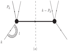
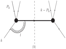
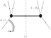
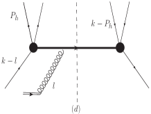
+h.c.

Figure 1: One loop order corrections to the fragmentation function of a quark into a meson pair in the spectator model. Where h.c. represents the hermitian conjugations of these diagrams.

We can model the correlator at one loop level provided with Fig.1 as:

$$\begin{aligned} \Delta_{a}^{q}(z,k_{T}^{2},\cos\theta,M_{h}^{2},\phi_{R})&=i\frac{C_{F}\alpha_{s}}{32\pi^{2}(1-z)P_{h}^{-}}\cdot\frac{|\vec{R}|}{M_{h}}\cdot\frac{(\not{k}+m)}{(k^{2}-m^{2})^{3}}\left(F^{s*}e^{-\frac{k^{2}}{\Lambda_{s}^{2}}}+F^{p*}e^{-\frac{k^{2}}{\Lambda_{p}^{2}}}\not{R}\right)(\not{k}-\not{P}_{h}+M_{s})\\ &\times\left(F^{s}e^{-\frac{k^{2}}{\Lambda_{s}^{2}}}+F^{p}e^{-\frac{k^{2}}{\Lambda_{p}^{2}}}\not{R}\right)(\not{k}+m)\int\frac{d^{4}\ell}{(2\pi)^{4}}\frac{\gamma^{\mu}(\not{k}-\not{\ell}+m)\gamma_{\mu}(\not{k}+m)}{((k-\ell)^{2}-m^{2}+i\varepsilon)(\ell^{2}+i\varepsilon)},\end{aligned}$$ (15)

$$\begin{aligned} \Delta_{b}^{q}(z,k_{T}^{2},\cos\theta,M_{h}^{2},\phi_{R})&=i\frac{C_{F}\alpha_{s}}{32\pi^{2}(1-z)P_{h}^{-}}\cdot\frac{|\vec{R}|}{M_{h}}\cdot\frac{(\not{k}+m)}{(k^{2}-m^{2})^{2}}\left(F^{s*}e^{-\frac{k^{2}}{\Lambda_{s}^{2}}}+F^{p*}e^{-\frac{k^{2}}{\Lambda_{p}^{2}}}\not{R}\right)(\not{k}-\not{P}_{h}+M_{s})\\ &\times\int\frac{d^{4}\ell}{(2\pi)^{4}}\frac{\gamma^{\mu}(\not{k}-\not{P}_{h}-\not{\ell}+M_{s})\Big{(}F^{s}e^{-\frac{k^{2}}{\Lambda_{s}^{2}}}+F^{p}e^{-\frac{k^{2}}{\Lambda_{p}^{2}}}\not{R}\Big{)}(\not{k}-\not{\ell}+m)\gamma_{\mu}(\not{k}+m)}{((k-P_{h}-\ell)^{2}-M_{s}^{2}+i\varepsilon)((k-\ell)^{2}-m^{2}+i\varepsilon)(\ell^{2}+i\varepsilon)},\end{aligned}$$ (16)

$$\begin{aligned} \Delta_{c}^{q}(z,k_{T}^{2},\cos\theta,M_{h}^{2},\phi_{R})&=i\frac{C_{F}\alpha_{s}}{32\pi^{2}(1-z)P_{h}^{-}}\cdot\frac{|\vec{R}|}{M_{h}}\cdot\frac{(\not{k}+m)}{(k^{2}-m^{2})^{2}}\left(F^{s*}e^{-\frac{k^{2}}{\Lambda_{s}^{2}}}+F^{p*}e^{-\frac{k^{2}}{\Lambda_{p}^{2}}}\not{R}\right)(\not{k}-\not{P}_{h}+M_{s})\\ &\times\left(F^{s}e^{-\frac{k^{2}}{\Lambda_{s}^{2}}}+F^{p}e^{-\frac{k^{2}}{\Lambda_{p}^{2}}}\not{R}\right)\int\frac{d^{4}\ell}{(2\pi)^{4}}\frac{(\not{k}+m)\gamma^{-}(\not{k}-\not{\ell}+m)}{((k-\ell)^{2}-m^{2}+i\varepsilon)(-\ell^{-}\pm i\varepsilon)(\ell^{2}+i\varepsilon)},\end{aligned}$$ (17)

$$\begin{aligned} \Delta_{d}^{q}(z,k_{T}^{2},\cos\theta,M_{h}^{2},\phi_{R})&=i\frac{C_{F}\alpha_{s}}{32\pi^{2}(1-z)P_{h}^{-}}\cdot\frac{|\vec{R}|}{M_{h}}\cdot\frac{(\not{k}+m)}{k^{2}-m^{2}}\left(F^{s*}e^{-\frac{k^{2}}{\Lambda_{s}^{2}}}+F^{p*}e^{-\frac{k^{2}}{\Lambda_{p}^{2}}}\not{R}\right)(\not{k}-\not{P}_{h}+M_{s})\\ &\times\int\frac{d^{4}\ell}{(2\pi)^{4}}\frac{\gamma^{-}(\not{k}-\not{P}_{h}-\not{\ell}+M_{s})\Big{(}F^{s}e^{-\frac{k^{2}}{\Lambda_{s}^{2}}}+F^{p}e^{-\frac{k^{2}}{\Lambda_{p}^{2}}}\not{R}\Big{)}(\not{k}-\not{\ell}+m)}{((k-P_{h}-\ell)^{2}-M_{s}^{2}+i\varepsilon)((k-\ell)^{2}-m^{2}+i\varepsilon)(-\ell^{-}\pm i\varepsilon)(\ell^{2}+i\varepsilon)}.\end{aligned}$$ (18)

In Eq.(15-18) we have applied the Feynman rule $1/(-\ell^{-}\pm i\varepsilon)$ for the eikonal propagator, as well as that for the vertex between the eikonal line and the gluon. Still in Eq.(15-18), in principle, the Gaussian form factors should depend on the loop momentum $\ell$. Following the choice made in Ref.Bacchetta et al. (2008a), we abandon this dependence and simply use $k^{2}$ in those form factors instead of $(k-\ell)^{2}$ in order to simplify the integration. This choice could give reasonable final results since the form factor is introduced to cut off the divergence. The same choice has also been adopted in Refs. Bacchetta et al. (2002, 2003); Amrath et al. (2005).

In general, there are two sources of $G_{1,OT}^{\perp}$ in each diagram at one loop level. One is the real part of the loop integral over $\ell$, coupled with the imaginary part of $F^{*}F^{p}$. The other is the imaginary part of the loop integral, combined with the real part of $F^{*}F^{p}$. The real part of the integral is presented as the usual loop integral adopting the Feynman parameterization. While for the imaginary part of the integral, we apply the Cutkosky cutting rules

$$\begin{aligned} \frac{1}{\ell^{2}+i\varepsilon}\to-2\pi i\delta(\ell^{2})\qquad\qquad\frac{1}{(k-\ell)^{2}+i\varepsilon}\to-2\pi i\delta((k-\ell)^{2}).\end{aligned}$$ (19)

Employing the above conventions, we reach the final result of $G_{1,OT}^{\perp}$

$$\begin{aligned} G_{1,OT}^{\perp a}&=0\\ G_{1,OT}^{\perp b}&=-\frac{1}{8\pi^{3}}\left[\frac{C_{F}\alpha_{s}M_{h}|\vec{R}|}{(1-z)}\cdot\Re[F^{s*}F^{p}]e^{-\frac{2k^{2}}{\Lambda_{sp}^{2}}}\right]\frac{1}{(k^{2}-m^{2})^{2}}C_{b}\\ &+\frac{1}{16\pi^{3}}\left[\frac{C_{F}\alpha_{s}M_{h}M_{s}|\vec{R}|}{(1-z)}\cdot\Im[F^{s*}F^{p}]e^{-\frac{2k^{2}}{\Lambda_{sp}^{2}}}\right]\frac{1}{(k^{2}-m^{2})^{2}}k^{2}\cdot C_{2}(k^{2},M_{h}^{2},2k^{2}+2M_{h}^{2}-M_{s}^{2},0,0,M_{s})\\ G_{1,OT}^{\perp c}&=0\\ G_{1,OT}^{\perp d}&=\frac{1}{2\pi^{3}}\left[\frac{C_{F}\alpha_{s}M_{h}M_{s}|\vec{R}|}{(1-z)}\cdot\Re[F^{s*}F^{p}]e^{-\frac{2k^{2}}{\Lambda_{sp}^{2}}}\right]\frac{1}{k^{2}-m^{2}}(-\mathcal{D}P_{h}^{-})\end{aligned}$$ (20)

with

$$\begin{aligned} C_{b}&=(4k^{2}M_{s}-2mk^{2}-4m^{3}-4m^{2}M_{s})\mathcal{A}+(2k^{2}M_{s}-mk^{2}+4M_{h}^{2}M_{s}-3mM_{h}^{2}-2m^{3}+2m^{2}M_{s}\\ &+3mM_{s}^{2}-4M_{s}^{3})\mathcal{B}+(2mk^{2}+2mM_{h}^{2}-2mM_{s}^{2})\mathcal{B}_{0}+4mM_{h}^{2}\mathcal{D}_{0}+(3mk^{2}-3m^{3})I_{2}+8m\mathcal{E}_{0},\end{aligned}$$ (21)

where $C_{2}$ is a three point one loop tensor integration defined as

$$\begin{aligned} &C_{2}(p_{1}^{2},p_{2}^{2},p_{3}^{2};m_{1}^{2},m_{2}^{2},m_{3}^{2})=\bigg{(}-2p_{1}^{2}B_{0}(p_{1}^{2},m_{1}^{2},m_{2}^{2})+(p_{1}^{2}+p_{2}^{2}-p_{3}^{2})B_{0}(p_{2}^{2},m_{2}^{2},m_{3}^{2})+(p_{1}^{2}-p_{2}^{2}+p_{3}^{2})B_{0}(p_{3}^{2},m_{1}^{2},m_{3}^{2})\\ &+[m_{1}^{2}(p_{1}^{2}+p_{2}^{2}-p_{3}^{2})+m_{2}^{2}(p_{1}^{2}-p_{2}^{2}+p_{3}^{2})+p_{1}^{2}(-2m_{3}^{2}-p_{1}^{2}+p_{2}^{2}+p_{3}^{2})]C_{0}(p_{1}^{2},p_{2}^{2},p_{3}^{2};m_{1}^{2},m_{2}^{2},m_{3}^{2})\bigg{)}\\ &\times\frac{1}{p_{1}^{4}-2(p_{2}^{2}+p_{3}^{2})p_{1}^{2}+(p_{2}^{2}-p_{3}^{2})^{2}}\end{aligned}$$ (22)

where the general defination of 2-point one-loop tensor integration $B_{0}$ is given by Ellis and Zanderighi (2008)

$$\begin{aligned} B_{0}(p_{1}^{2};m_{1}^{2},m_{2}^{2})=\frac{1}{i\pi^{2}}\int d^{4}l\frac{1}{(l^{2}-m_{1}^{2}+i\varepsilon)((l+q_{1})^{2}-m_{2}^{2}+i\varepsilon)}\end{aligned}$$ (23)

and 3-point one-loop tensor integration $C_{0}$ is denoted as Ellis and Zanderighi (2008)

$$\begin{aligned} C_{0}(p_{1}^{2},p_{2}^{2},p_{3}^{2};m_{1}^{2},m_{2}^{2},m_{3}^{2})=\frac{1}{i\pi^{2}}\int d^{4}\ell\frac{1}{(\ell^{2}-m_{1}^{2}+i\varepsilon)((\ell+q_{1})^{2}-m_{2}^{2}+i\varepsilon)((\ell+q_{2})^{2}-m_{3}^{2}+i\varepsilon)}\end{aligned}$$ (24)

with $q_{n}\equiv\sum_{i=1}^{n}p_{i}$ and $q_{0}=0$. The coefficients $\mathcal{A}$ and $\mathcal{B}$ denote the following functions

$$\begin{aligned} \mathcal{A}&=\frac{I_{1}}{\lambda(M_{h},M_{s})}\left[2k^{2}(k^{2}-M_{s}^{2}-M_{h}^{2})\frac{I_{2}}{\pi}+(k^{2}+M_{h}^{2}-M_{s}^{2})\right]\\ \mathcal{B}&=-\frac{2k^{2}}{\lambda(M_{h}^{2},M_{s}^{2})}I_{1}\left[1+\frac{k^{2}+M_{s}^{2}-M_{h}^{2}}{\pi}I_{2}\right]\end{aligned}$$ (25)

which originate from the decomposition of the following integral Lu and Schmidt (2015)

$$\begin{aligned} \int d^{4}\ell\frac{\ell^{\mu}\delta(\ell^{2})\delta[(k-\ell)^{2}-m^{2}]}{(k-P_{h}-\ell)^{2}-M_{s}^{2}}=\mathcal{A}k^{\mu}+\mathcal{B}P_{h}^{\mu}.\end{aligned}$$ (26)

The functions $I_{i}$ represent the results of the following integrals

$$\begin{aligned} I_{1}&=\int d^{4}\ell\delta(\ell^{2})\delta[(k-\ell)^{2}-m^{2}]=\frac{\pi}{2k^{2}}(k^{2}-m^{2})\\ I_{2}&=\int d^{4}\ell\frac{\delta(\ell^{2})\delta[(k-\ell)^{2}-m^{2}]}{(k-\ell-P_{h})^{2}-M_{s}^{2}}=\frac{\pi}{2\sqrt{\lambda(M_{h},M_{s})}}\ln\left(1-\frac{2\sqrt{\lambda(M_{h},M_{s})}}{k^{2}-M_{h}^{2}+M_{s}^{2}+\sqrt{\lambda(M_{h},M_{s})}}\right)\\ I_{3}&=\int d^{4}\ell\frac{\delta(\ell^{2})\delta((k-\ell)^{2}-m^{2})}{-\ell^{-}+i\varepsilon}\\ I_{4}&=\int d^{4}\ell\frac{\delta(\ell^{2})\delta((k-\ell)^{2}-m^{2})}{(-\ell^{-}+i\varepsilon)((k-P_{h}-\ell)^{2}-M_{s}^{2})}\end{aligned}$$ (27)

with $\lambda(M_{h},M_{s})=[k^{2}-(M_{h}+M_{s})^{2}][k^{2}-(M_{h}-M_{s})^{2}]$. The function $\mathcal{D}$ satisfies the following relation

$$\begin{aligned} P_{h}^{-}\mathcal{D}&=-\frac{I_{34}}{2zk_{T}^{2}}-\frac{1}{2zk_{T}^{2}}\left((1-2z)k^{2}+M_{h}^{2}-M_{s}^{2}\right)I_{2},\end{aligned}$$ (28)

where $I_{34}$ is the linear combination of $I_{3}$ and $I_{4}$

$$\begin{aligned} I_{34}=k^{-}(I_{3}+(1-z)(k^{2}-m^{2})I_{4})=\pi\ln\frac{\sqrt{k^{2}}(1-z)}{M_{s}}.\end{aligned}$$ (29)

In addition, the function $\mathcal{B}_{0}$ and $\mathcal{D}_{0}$ come from the decomposition

$$\begin{aligned} \int d^{4}\ell\frac{\ell^{\mu}\ell^{\nu}\delta(\ell^{2})\delta((k-\ell)^{2}-m^{2})}{(k-p-\ell)^{2}-M_{s}^{2}}&=k^{\mu}k^{\nu}\mathcal{A}_{0}+k^{\mu}p^{\nu}\mathcal{B}_{0}+p^{\mu}k^{\nu}\mathcal{C}_{0}+p^{\mu}p^{\nu}\mathcal{D}_{0}+g^{\mu\nu}\mathcal{E}_{0},\end{aligned}$$ (30)

where

$$\begin{aligned} \mathcal{B}_{0}&=\frac{1}{2}\frac{(k^{2}-m^{2})(\mathcal{A}k^{2}+3\mathcal{B}k^{2}+\mathcal{A}M_{h}^{2}-\mathcal{B}M_{h}^{2}-\mathcal{A}M_{s}^{2}-3\mathcal{B}M_{s}^{2})}{k^{4}-2k^{2}M_{h}^{2}-2k^{2}M_{s}^{2}+M_{h}^{4}-2M_{h}^{2}M_{s}^{2}+M_{s}^{4}}\\ \mathcal{D}_{0}&=-\frac{(k^{2}-m^{2})(\mathcal{A}k^{2}+2\mathcal{B}k^{2}-\mathcal{B}M_{h}^{2}+\mathcal{B}M_{s}^{2})}{k^{4}-2k^{2}M_{h}^{2}-2k^{2}M_{s}^{2}+M_{h}^{4}-2M_{h}^{2}M_{s}^{2}+M_{s}^{4}}\\ \mathcal{E}_{0}&=-\frac{1}{4}(k^{2}-m^{2})(\mathcal{A}+\mathcal{B})\end{aligned}$$ (31)

IV The $\sin(\phi_{h}-\phi_{R})$ asymmetry of dihadron production in SIDIS

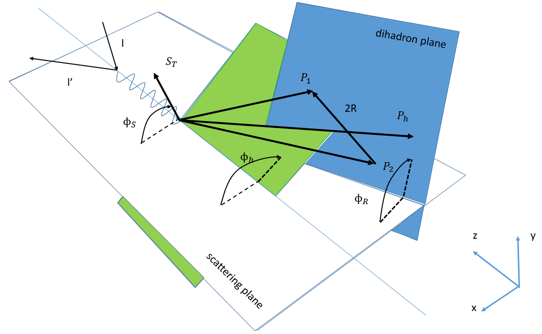
Figure 2: Angle definitions involved in the measurement of the single longitudinal spin asymmetry in SIDIS production of two hadrons.

The reference system in Fig.2 is our starting point in which the virtual photon transverse momentum is set to $\vec{q}_{T}=0$. But in our work, the virtual photon has a nonvanishing transverse momentum $\vec{q}_{T}$. We align the $\hat{z}$ axis opposite to the direction of the virtual photon for the transverse momentum dependence case and, the outgoing hadron has a nonvanishing transverse momentum defined as $\vec{P}_{h\perp}=-z\vec{q}_{T}$. Then we consider the dihadron SIDIS production

$$\begin{aligned} \mu(\ell)+p^{\rightarrow}(P)\to\mu(\ell^{\prime})+h^{+}(P_{1})+h^{-}(P_{2})+X,\end{aligned}$$ (32)

where a unpolarized muon with momentum $\ell$ scatters off a longitudinally polarized target nucleon with mass $M$, polarization $S$ and momentum $P$, via the exchange of a virtual photon with momentum $q=\ell-\ell^{\prime}$. Inside the target, the photon hits the active quark with momentum $p$ and the final state quark with momentum $k=p+q$ then fragments into two leading unpolarized hadrons with mass $M_{1},M_{2}$, and momenta $P_{1},P_{2}$. To present the differential cross section with respect to dihadron-dependent structure function, we define the following kinematic invariants:

$$\begin{aligned} x&=\frac{k^{+}}{P^{+}}\qquad y=\frac{P\cdot q}{P\cdot\ell}\qquad z=\frac{P_{h}^{-}}{k^{-}}=z_{1}+z_{2}\\ z_{i}&=\frac{P_{i}^{-}}{k^{-}}\qquad Q^{2}=-q^{2}\qquad s=(P+\ell)^{2}\\ P_{h}&=P_{1}+P_{2}\qquad R=\frac{P_{1}-P_{2}}{2}\qquad M_{h}^{2}=P_{h}^{2}.\end{aligned}$$ (33)

The light-cone fraction of target momentum carried by the initial quark is denoted by $x$, $z_{i}$ expresses the light-cone fraction of hadron $h_{i}$ in terms of the fragmented quark. The light-cone fraction of fragmenting quark momentum carried by the final hadron pair is defined by $z$. Moreover, the invariant mass, the total momentum and the relative momentum of the hadron pair are denoted by $M_{h}$, $P_{h}$ and $R$, respectively.

We will consider the SIDIS process with unpolarized muons off longitudinally polarized nucleon target. Using TMD factorization approach and denoting $A(y)=1-y+\frac{y^{2}}{2}$, the differential cross section for this process reads Radici et al. (2002)

$$\begin{aligned} \displaystyle\frac{d^{9}\sigma_{UU}}{dxdydzd\phi_{S}d\phi_{h}d\phi_{R}d\cos\theta d\vec{P}_{h\perp}^{2}dM_{h}^{2}}=\frac{\alpha^{2}}{2\pi sxy^{2}}A(y)\sum_{q}e_{q}^{2}\mathcal{I}[f_{1}^{q}D_{1,OO}^{q}]\end{aligned}$$ (34)

and

$$\begin{aligned} \displaystyle\frac{d^{9}\sigma_{UL}}{dxdydzd\phi_{S}d\phi_{h}d\phi_{R}d\cos\theta d\vec{P}_{h\perp}^{2}dM_{h}^{2}}&=\frac{\alpha^{2}}{2\pi sxy^{2}}A(y)\sum_{q}e_{q}^{2}\bigg{\{}\sin\theta\sin(\phi_{h}-\phi_{R})\mathcal{I}\left[\frac{\vec{k}_{T}\cdot\hat{P}_{h\perp}}{M_{h}}g_{1L}^{q}\left(\frac{|\vec{R}|}{M_{h}}G_{1,OT}^{\perp}\right)\right]\\ &+\sin 2\theta\sin(\phi_{h}-\phi_{R})\mathcal{I}\left[\frac{\vec{k}_{T}\cdot\hat{P}_{h\perp}}{M_{h}}g_{1L}^{q}\left(\frac{|\vec{R}|}{2M_{h}}G_{1,LT}^{\perp}\right)\right]\bigg{\}},\end{aligned}$$ (35)

where $\phi_{R}$ and $\phi_{S}$ are the azimuthal angles of $\vec{R}_{T}$ and $\vec{S}_{T}$ with respect to the lepton scattering plane. $\hat{P}_{h\perp}$ satisfies $\hat{P}_{h\perp}=\vec{P}_{h\perp}/|\vec{P}_{h\perp}|$. For convenience, we have indicated the unpolarized or longitudinally polarized states of the beam or the target with the labels $U$ and $L$, respectively. The structure functions occuring in Eqs.(34-35) are written as weighted convolutions of the form

$$\begin{aligned} \mathcal{I}[f]=\int d^{2}\vec{p}_{T}d^{2}\vec{k}_{T}\delta\left(\vec{p}_{T}-\vec{k}_{T}-\frac{\vec{P}_{h\perp}}{z}\right)[f].\end{aligned}$$ (36)

In Eq.(34), $f_{1}^{q}$ and $D_{1,OO}^{q}$ are the unpolarized PDF and unpolarized DiFF with flavor $q$. In Eq.(35), $g_{1L}^{q}$ is a twist-2 distribution function coupled with the T-odd DiFF $G_{1,OT}^{\perp}$ and $G_{1,LT}^{\perp}$ respectively. In principle, both DiFFs contribute to the $\sin(\phi_{h}-\phi_{R})$ azimuthal asymmetry in SIDIS. However, to access the asymmetry one must do the integration with respect to $\theta$ and we have $\int_{-1}^{1}\sin 2\theta d\cos\theta=0$ for the latter contribution. Thus the contribution including $G_{1,LT}^{\perp}$ vanishes and the $\sin(\phi_{h}-\phi_{R})$ asymmetry of the considered process can be expressed as

$$\begin{aligned} A_{UL}^{\sin(\phi_{h}-\phi_{R})}&=&\displaystyle\frac{\pi}{4}\frac{\sum_{q}e_{q}^{2}\mathcal{I}\left[\frac{\vec{k}_{T}\cdot\hat{P}_{h\perp}}{M_{h}}g_{1L}^{q}\left(\frac{|\vec{R}|}{M_{h}}G_{1,OT}^{\perp}\right)\right]}{\sum_{q}e_{q}^{2}\int\mathcal{I}[f_{1}^{q}D_{1,OO}^{q}]}.\end{aligned}$$ (37)

V Numerical results

In order to fix the parameters of the spectator model, the authors of Ref. Bacchetta and Radici (2006) compare it with the output of the PYTHIA event generator Sjostrand et al. (2001) adopted for HERMES. The values of the parameters obtained by the fit are:

$$\alpha_{s} =2.60\ \text{GeV} \beta_{s}=-0.751 \gamma_{s}=-0.193$$

$$\alpha_{p} =7,07\ \text{GeV} \beta_{p}=-0.038 \gamma_{p}=-0.085$$

$$f_{s} =1197\ \text{GeV}^{-1} f_{\rho}=93.5 f_{\omega}=0.63$$

$$f_{\omega}^{\prime} =75.2 M_{s}=2.97M_{h} m=0.0\ \text{GeV},$$

where we have adopted the same choice as in Ref. Bacchetta and Radici (2006) for the quark mass $m$ fixed to be zero GeV. It’s desired to mention that these model parameters are obtained by comparing the theoretical model with the PITHIA event generator adopted for the HERMES kinematics. In the following we will make predictions in COMPASS and EIC kinematics, thus there are uncertainties with respect to the model parameters. In this paper, we make a rough consideration by ignoring such uncertainties. Furthermore, we make a preliminary estimate for choosing the strong coupling $\alpha_{s}\approx 0.3$.

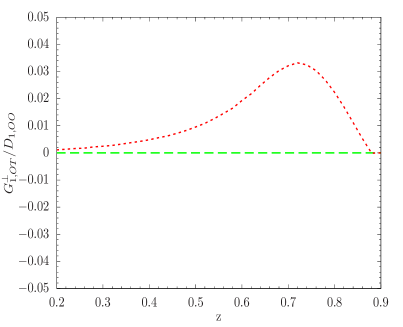
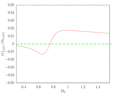
Figure 3: The DiFF $G^{\perp}_{1,OT}$ as functions of $z$ (left panel) and $M_{h}$ (right panel) in the spectator model, normalized by the unpolarized DiFF $D_{1,OO}$.

We map out the ratio between $G^{\perp}_{1,OT}$ and $D_{1,OO}$ as a function of $z$ or $M_{h}$, integrated over the region $0.3\ \text{GeV}<M_{h}<1.6\ \text{GeV}$ or $0.2<z<0.9$ in the left panel and right panel of Fig.3 respectively. Comparing with the unpolarized DiFF $D_{1,OO}$, the $G^{\perp}_{1,OT}$ is two order of magnitude smaller and we can find a break point located nearly in $M_{h}=0.8$.

Then we present the numerical results of the $\sin(\phi_{h}-\phi_{R})$ azimuthal asymmetry in the SIDIS process with unpolarized muons off longitudinally polarized nucleon target. According to isospin symmetry we have the conclusion that the fragmentation correlators for processes $u\to\pi^{+}\pi^{-}X$, $\bar{d}\to\pi^{+}\pi^{-}X$, $d\to\pi^{-}\pi^{+}X$ and $\bar{u}\to\pi^{-}\pi^{+}X$ are the same. Thus by transforming the sign of $\vec{R}$, equivalently changing $\theta\to\pi-\theta$ and $\phi\to\phi+\pi$, the DiFF $G_{1,OT}^{\perp}$ which depends linearly on $R$ coming from $d\to\pi^{-}\pi^{+}X$ and $\bar{u}\to\pi^{-}\pi^{+}X$ processes has an additional minus sign comparing to the $u\to\pi^{+}\pi^{-}X$ process. When expanding the flavor sum in the numerator of Eq.(37), we apply the isospin symmetry to the DiFF $G_{1}^{\perp}$. Furthermore, in principle sea quark distributions can be generated via perturbative QCD evolution and they are zero at the model scale. In this paper, we make a rough consideration by ignoring QCD evolution, which leads to zero antiquark PDFs $f_{1}$ and $g_{1L}$. The expressions of the $x$-dependent, $z$-dependent and $M_{h}$-dependent $\sin(\phi_{h}-\phi_{R})$ asymmetry can be adopted from Eq.(37) as follows

$$\begin{aligned} &\displaystyle A_{UL}^{\sin(\phi_{h}-\phi_{R})}(x)=\frac{\int dz2M_{h}dM_{h}d\cos\theta d^{2}\vec{P}_{h\perp}d^{2}\vec{p}_{T}d^{2}\vec{k}_{T}\delta\left(\vec{p}_{T}-\vec{k}_{T}-\frac{\vec{P}_{h\perp}}{z}\right)(4g_{1L}^{u}(\vec{p}_{T}^{2})-g_{1L}^{d}(\vec{p}_{T}^{2}))G_{1,OT}^{\perp}(\vec{k}_{T}^{2})\sin\theta\frac{\vec{k}_{T}\cdot\vec{P}_{h\perp}|\vec{R}|}{2M_{h}^{2}|\vec{P}_{h\perp}|}}{\int dz2M_{h}dM_{h}d\cos\theta d^{2}\vec{P}_{h\perp}d^{2}\vec{p}_{T}d^{2}\vec{k}_{T}\delta\left(\vec{p}_{T}-\vec{k}_{T}-\frac{\vec{P}_{h\perp}}{z}\right)(4f_{1}^{u}(\vec{p}_{T}^{2})+f_{1}^{d}(\vec{p}_{T}^{2}))D_{1,OO}(\vec{k}_{T}^{2})}\\ &\displaystyle A_{UL}^{\sin(\phi_{h}-\phi_{R})}(z)=\frac{\int dx2M_{h}dM_{h}d\cos\theta d^{2}\vec{P}_{h\perp}d^{2}\vec{p}_{T}d^{2}\vec{k}_{T}\delta\left(\vec{p}_{T}-\vec{k}_{T}-\frac{\vec{P}_{h\perp}}{z}\right)(4g_{1L}^{u}(\vec{p}_{T}^{2})-g_{1L}^{d}(\vec{p}_{T}^{2}))G_{1,OT}^{\perp}(\vec{k}_{T}^{2})\sin\theta\frac{\vec{k}_{T}\cdot\vec{P}_{h\perp}|\vec{R}|}{2M_{h}^{2}|\vec{P}_{h\perp}|}}{\int dx2M_{h}dM_{h}d\cos\theta d^{2}\vec{P}_{h\perp}d^{2}\vec{p}_{T}d^{2}\vec{k}_{T}\delta\left(\vec{p}_{T}-\vec{k}_{T}-\frac{\vec{P}_{h\perp}}{z}\right)(4f_{1}^{u}(\vec{p}_{T}^{2})+f_{1}^{d}(\vec{p}_{T}^{2}))D_{1,OO}(\vec{k}_{T}^{2})}\\ &\displaystyle A_{UL}^{\sin(\phi_{h}-\phi_{R})}(M_{h})=\frac{\int dxdzd\cos\theta d^{2}\vec{P}_{h\perp}d^{2}\vec{p}_{T}d^{2}\vec{k}_{T}\delta\left(\vec{p}_{T}-\vec{k}_{T}-\frac{\vec{P}_{h\perp}}{z}\right)(4g_{1L}^{u}(\vec{p}_{T}^{2})-g_{1L}^{d}(\vec{p}_{T}^{2}))G_{1,OT}^{\perp}(\vec{k}_{T}^{2})\sin\theta\frac{\vec{k}_{T}\cdot\vec{P}_{h\perp}|\vec{R}|}{2M_{h}^{2}|\vec{P}_{h\perp}|}}{\int dxdzd\cos\theta d^{2}\vec{P}_{h\perp}d^{2}\vec{p}_{T}d^{2}\vec{k}_{T}\delta\left(\vec{p}_{T}-\vec{k}_{T}-\frac{\vec{P}_{h\perp}}{z}\right)(4f_{1}^{u}(\vec{p}_{T}^{2})+f_{1}^{d}(\vec{p}_{T}^{2}))D_{1,OO}(\vec{k}_{T}^{2})},\end{aligned}$$ (38)

where the TMD DiFF $D_{1,OO}$ has been worked out and listed as

$$\begin{aligned} D_{1,OO}(z,\vec{k}_{T}^{2},M_{h})=&\frac{4\pi|\vec{R}|}{256\pi^{3}M_{h}z(1-z)(k^{2}-m^{2})^{2}}\bigg{\{}4|F^{s}|^{2}e^{-\frac{2k^{2}}{\Lambda_{s}^{2}}}(zk^{2}-M_{h}^{2}-m^{2}z+m^{2}+2mM_{s}+M_{s}^{2})\\ &-4|F^{p}|^{2}e^{-\frac{2k^{2}}{\Lambda_{p}^{2}}}|\vec{R}|^{2}(-zk^{2}+M_{h}^{2}+m^{2}(z-1)+2mM_{s}-M_{s}^{2})\\ &+\frac{4}{3}|F^{p}|^{2}e^{-\frac{2k^{2}}{\Lambda_{p}^{2}}}|\vec{R}|^{2}\bigg{[}4\left(\frac{M_{h}}{2z}-z\frac{k^{2}+\vec{k}_{T}^{2}}{2M_{h}}\right)^{2}+2z\frac{k^{2}-m^{2}}{M_{h}}\left(\frac{M_{h}}{2z}-z\frac{k^{2}+\vec{k}_{T}^{2}}{2M_{h}}\right)\bigg{]}\bigg{\}}.\end{aligned}$$ (39)

As for the twist-2 PDFs $f_{1}$ and $g_{1}$, we apply the same spectator model results Bacchetta et al. (2008b) for uniformity. To perform numerical calculation for the $\sin(\phi_{h}-\phi_{R})$ asymmetry in dihadron SIDIS at the COMPASS kinematics, we adopt the following kinematical cuts Sirtl (2016)

$$\begin{aligned} &\sqrt{s}=17.4\ \text{GeV}\qquad 0.003<x<0.4\qquad 0.1<y<0.9\qquad 0.2<z<0.9\\ &0.3\text{GeV}<M_{h}<1.6\ \text{GeV}\qquad Q^{2}>1\ \text{GeV}^{2}\qquad W>5\ \text{GeV},\end{aligned}$$ (40)

where $W$ is the invariant mass of photon-nucleon system with $W^{2}=(P+q)^{2}\approx\frac{1-x}{x}Q^{2}$.

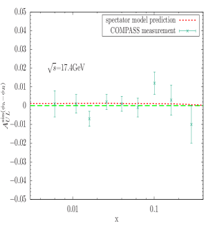
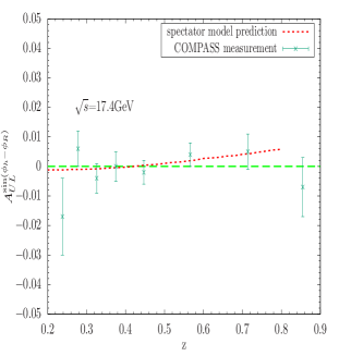
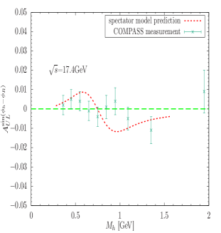
Figure 4: The $\sin(\phi_{h}-\phi_{R})$ azimuthal asymmetry in the SIDIS process of unpolarized muons off longitudinally polarized nucleon target as a functions of $x$ (left panel), $z$ (central panel) and $M_{h}$ (right panel) at COMPASS. The full circles with error bars show the preliminary COMPASS data Sirtl (2017) for comparison. The dashed curves denote the model prediction.

Our main results in this work are our predictions for the $\sin(\phi_{h}-\phi_{R})$ azimuthal asymmetry in the SIDIS process with unpolarized muons off longitudinally polarized nucleon target, as shown in Fig.4. The $x$-, $z$- and $M_{h}$-dependent asymmetries are depicted in the left, central and right panels of the figure, respectively. The dashed lines represent our model predictions. The full circles with error bars show the preliminary COMPASS data for comparison. We can find that the model predictions give a good description of the COMPASS preliminary data being compariable with zero.

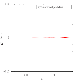
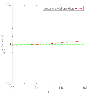
Figure 5: The $\sin(\phi_{h}-\phi_{R})$ azimuthal asymmetry in the SIDIS process of unpolarized muons off longitudinally polarized nucleon target as a functions of $x$ (left panel), $z$ (central panel) and $M_{h}$ (right panel) at the EIC ($\sqrt{s}=45$GeV). The dashed curves denote the model prediction.

Then, to make a further comparison, we also obtain the $\sin(\phi_{h}-\phi_{R})$ asymmetry at the future EIC. Such a facility might be picture-perfect to study this observable. We settle on the following EIC kinematical cuts Accardi et al. (2016):

$$\begin{aligned} &\sqrt{s}=45\ \text{GeV}\qquad 0.001<x<0.4\qquad 0.01<y<0.95\qquad 0.2<z<0.8\\ &0.3\ \text{GeV}<M_{h}<1.6\ \text{GeV}\qquad Q^{2}>1\ \text{GeV}^{2}\qquad W^{2}>10\ \text{GeV}^{2}.\end{aligned}$$ (41)

The $x$-, $z$- and $M_{h}$-dependent asymmetries are plotted in the left, central, and right panels in Fig.5. We find that the overall tendency of the asymmetry at the EIC is similar to that at COMPASS. Since the size of the asymmetry is lightly smaller than that at COMPASS, the results are still compariable with zero at the kinematics of EIC. It is also possible to conceive a set of kinematical cuts reach for the future EIC but not for COMPASS to observe if the future EIC could bring new information on asymmetries. We can reach the following EIC kinematical cuts for a future EIC:

$$\begin{aligned} &\sqrt{s}=100\ \text{GeV}\qquad 0.001<x<0.7\qquad 0.01<y<0.95\qquad 0.2<z<0.8\\ &0.3\ \text{GeV}<M_{h}<1.6\ \text{GeV}\qquad Q^{2}>25\text{GeV}^{2}\qquad W>10\ \text{GeV}.\end{aligned}$$ (42)

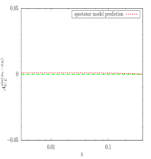
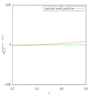
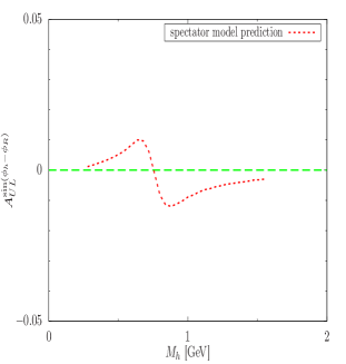
Figure 6: The $\sin(\phi_{h}-\phi_{R})$ azimuthal asymmetry in the SIDIS process of unpolarized muons off longitudinally polarized nucleon target as a functions of $x$ (left panel), $z$ (central panel) and $M_{h}$ (right panel) at the future EIC ($\sqrt{s}=100$GeV). The dashed curves denote the model prediction.

The $x$-, $z$- and $M_{h}$-dependent asymmetries are plotted in the left, central, and right panels in Fig.6. We find that the asymmeties are not prompted by the future EIC kinematics.

In addition, the available theoretical bounds on $G_{1}^{\perp}$(see Eq.(55) of Radici et al. (2002)) would give a much larger asymmetry, and therefore the COMPASS data and the present predictions strongly constrain this DiFF within their uncertainty.

Finally, the expected size of $A_{UL}^{\sin(\phi_{h}-\phi_{R})}$ in the NJL quark model Matevosyan et al. (2013, 2014, 2017); Matevosyan et al. (2018a) is zero, which is basically consistent with the spectator model result. This conclusion can be reached by considering Eq.(12) of Ref. Matevosyan et al. (2018b) together with both Eq.(19) and Eq.(26) in Ref. Matevosyan et al. (2018a). In addition, Ref. Matevosyan et al. (2018b) proposed a measurement which will permit us to access the helicity-dependent DiFF in forward two-hadron production in SIDIS. We will make a prediction for this measurement in a upcoming work using the spectator model result of helicity-dependent DiFFs.

VI Conclusion

In this work, we have considered the single spin asymmetry with a $\sin(\phi_{h}-\phi_{R})$ modulation of dihadron production in SIDIS. With the spectator model result for $D_{1,OO}$ at hand, we worked out the T-odd DiFF $G_{1,OT}^{\perp}$ by considering the real and imaginary loop contributions. Using the partial wave expansion, we found that $G_{1,OT}^{\perp}$ comes from the interference contribution of the $s$- and $p$-waves. By using the numerical results of the DiFFs and PDFs, we present the prediction for the $\sin(\phi_{h}-\phi_{R})$ asymmetry and compare it with the COMPASS measurements. Our result yields a good description of the vanished COMPASS data.

References

Konishi et al. (1979)
K. Konishi,
A. Ukawa, and
G. Veneziano,
Nucl. Phys. B157,
45 (1979).
Vendramin (1981a)
I. Vendramin, in
In *Wuerzburg 1981, Proceedings, Problems In Gauge
Theories*, 29-52 (1981a).
Vendramin (1981b)
I. Vendramin,
Nuovo Cim. A66,
339 (1981b).
Ceccopieri et al. (2007)
F. A. Ceccopieri,
M. Radici, and
A. Bacchetta,
Phys. Lett. B650,
81 (2007), eprint hep-ph/0703265.
Collins and Ladinsky (1994)
J. C. Collins and
G. A. Ladinsky
(1994), eprint hep-ph/9411444.
Bianconi
et al. (2000a)
A. Bianconi,
S. Boffi,
R. Jakob, and
M. Radici,
Phys. Rev. D62,
034008 (2000a),
eprint hep-ph/9907475.
Collins et al. (1994)
J. C. Collins,
S. F. Heppelmann,
and G. A.
Ladinsky, Nucl. Phys.
B420, 565 (1994),
eprint hep-ph/9305309.
Jaffe et al. (1998)
R. L. Jaffe,
X.-m. Jin, and
J. Tang,
Phys. Rev. Lett. 80,
1166 (1998), eprint hep-ph/9709322.
Radici et al. (2002)
M. Radici,
R. Jakob, and
A. Bianconi,
Phys. Rev. D65,
074031 (2002), eprint hep-ph/0110252.
Bacchetta and Radici (2004)
A. Bacchetta and
M. Radici,
Phys. Rev. D69,
074026 (2004), eprint hep-ph/0311173.
Gliske et al. (2014)
S. Gliske,
A. Bacchetta,
and M. Radici,
Phys. Rev. D90,
114027 (2014), [Erratum:
Phys. Rev.D91,no.1,019902(2015)], eprint 1408.5721.
Collins (1993)
J. C. Collins,
Nucl. Phys. B396,
161 (1993), eprint hep-ph/9208213.
Bacchetta and Radici (2003)
A. Bacchetta and
M. Radici,
Phys. Rev. D67,
094002 (2003), eprint hep-ph/0212300.
Vossen et al. (2011)
A. Vossen et al.
(Belle), Phys. Rev. Lett.
107, 072004
(2011), eprint 1104.2425.
Courtoy et al. (2012)
A. Courtoy,
A. Bacchetta,
M. Radici, and
A. Bianconi,
Phys. Rev. D85,
114023 (2012), eprint 1202.0323.
Bacchetta et al. (2011)
A. Bacchetta,
A. Courtoy, and
M. Radici,
Phys. Rev. Lett. 107,
012001 (2011), eprint 1104.3855.
Bacchetta et al. (2013)
A. Bacchetta,
A. Courtoy, and
M. Radici,
JHEP 03, 119
(2013), eprint 1212.3568.
Radici et al. (2015)
M. Radici,
A. Courtoy,
A. Bacchetta,
and
M. Guagnelli,
JHEP 05, 123
(2015), eprint 1503.03495.
Radici et al. (2016)
M. Radici,
A. M. Ricci,
A. Bacchetta,
and
A. Mukherjee,
Phys. Rev. D94,
034012 (2016), eprint 1604.06585.
Radici and Bacchetta (2018)
M. Radici and
A. Bacchetta,
Phys. Rev. Lett. 120,
192001 (2018), eprint 1802.05212.
Bianconi
et al. (2000b)
A. Bianconi,
S. Boffi,
R. Jakob, and
M. Radici,
Phys. Rev. D62,
034009 (2000b),
eprint hep-ph/9907488.
Bacchetta and Radici (2006)
A. Bacchetta and
M. Radici,
Phys. Rev. D74,
114007 (2006), eprint hep-ph/0608037.
Bacchetta et al. (2009)
A. Bacchetta,
F. A. Ceccopieri,
A. Mukherjee,
and M. Radici,
Phys. Rev. D79,
034029 (2009), eprint 0812.0611.
Matevosyan et al. (2013)
H. H. Matevosyan,
A. W. Thomas,
and W. Bentz,
Phys. Rev. D88,
094022 (2013), eprint 1310.1917.
Matevosyan et al. (2014)
H. H. Matevosyan,
A. Kotzinian,
and A. W.
Thomas, Phys. Lett.
B731, 208 (2014),
eprint 1312.4556.
Matevosyan et al. (2017)
H. H. Matevosyan,
A. Kotzinian,
and A. W.
Thomas, Phys. Rev.
D96, 074010
(2017), eprint 1707.04999.
Matevosyan
et al. (2018a)
H. H. Matevosyan,
A. Kotzinian,
and A. W.
Thomas, Phys. Rev.
D97, 014019
(2018a), eprint 1709.08643.
Airapetian et al. (2008)
A. Airapetian
et al. (HERMES),
JHEP 06, 017
(2008), eprint 0803.2367.
Adolph et al. (2012)
C. Adolph et al.
(COMPASS), Phys. Lett.
B713, 10 (2012),
eprint 1202.6150.
Adolph et al. (2014)
C. Adolph et al.
(COMPASS), Phys. Lett.
B736, 124 (2014),
eprint 1401.7873.
Sirtl (2017)
S. Sirtl, in
22nd International Symposium on Spin Physics (SPIN
2016) Urbana, IL, USA, September 25-30, 2016 (2017),
eprint 1702.07317.
Eidelman et al. (2004)
S. Eidelman et al.
(Particle Data Group), Phys.
Lett. B592, 1
(2004).
Bacchetta
et al. (2008a)
A. Bacchetta,
L. P. Gamberg,
G. R. Goldstein,
and
A. Mukherjee,
Phys. Lett. B659,
234 (2008a),
eprint 0707.3372.
Bacchetta et al. (2002)
A. Bacchetta,
R. Kundu,
A. Metz, and
P. J. Mulders,
Phys. Rev. D65,
094021 (2002), eprint hep-ph/0201091.
Bacchetta et al. (2003)
A. Bacchetta,
A. Metz, and
J.-J. Yang,
Phys. Lett. B574,
225 (2003), eprint hep-ph/0307282.
Amrath et al. (2005)
D. Amrath,
A. Bacchetta,
and A. Metz,
Phys. Rev. D71,
114018 (2005), eprint hep-ph/0504124.
Ellis and Zanderighi (2008)
R. K. Ellis and
G. Zanderighi,
JHEP 02, 002
(2008), eprint 0712.1851.
Lu and Schmidt (2015)
Z. Lu and
I. Schmidt,
Phys. Lett. B747,
357 (2015), eprint 1501.04379.
Sjostrand et al. (2001)
T. Sjostrand,
P. Eden,
C. Friberg,
L. Lonnblad,
G. Miu,
S. Mrenna, and
E. Norrbin,
Comput. Phys. Commun. 135,
238 (2001), eprint hep-ph/0010017.
Bacchetta
et al. (2008b)
A. Bacchetta,
F. Conti, and
M. Radici,
Phys. Rev. D78,
074010 (2008b),
eprint 0807.0323.
Sirtl (2016)
S. Sirtl,
Azimuthal asymmetries in semi-inclusive deep-inelastic
hadron muoproduction on longitudinally polarized protons, Ph.D. thesis,
University of Freiburg (2016).
Accardi et al. (2016)
A. Accardi et al.,
Eur. Phys. J. A52,
268 (2016), eprint 1212.1701.
Matevosyan
et al. (2018b)
H. H. Matevosyan,
A. Kotzinian,
and A. W.
Thomas, Phys. Rev. Lett.
120, 252001
(2018b), eprint 1712.06384.