Machine learning based non-Newtonian fluid model with molecular fidelity

Abstract

We introduce a machine-learning-based framework for constructing continuum non-Newtonian fluid dynamics model directly from a micro-scale description. Dumbbell polymer solutions are used as examples to demonstrate the essential ideas. To faithfully retain molecular fidelity, we establish a micro-macro correspondence via a set of encoders for the micro-scale polymer configurations and their macro-scale counterparts, a set of nonlinear conformation tensors. The dynamics of these conformation tensors can be derived from the micro-scale model and the relevant terms can be parametrized using machine learning. The final model, named the deep non-Newtonian model (DeePN²), takes the form of conventional non-Newtonian fluid dynamics models, with a new form of the objective tensor derivative. Both the formulation of the dynamic equation and the neural network representation rigorously preserve the rotational invariance, which ensures the admissibility of the constructed model. Numerical results demonstrate the accuracy of DeePN², where models based on empirical closures show limitations.

I Introduction

Accurate modeling of non-Newtonian fluid flows has been a long-standing problem. Existing hydrodynamic models have to resort to ad hoc assumptions either directly at the macro-scale level when writing down constitutive laws, or as closure assumptions when deriving macro-scale models from some underlying micro-scale description. A variety of empirical constitutive models Larson (1988); Owens and Phillips (2002) of both integral and derivative types have been developed, including Oldroyd-B Oldroyd and Wilson (1950), Giesekus Giesekus (1982), finite extensible nonlinear elastic Peterlin (FENE-P) Peterlin (1966); Bird et al. (1980), Rivlin-Sawyers Rivlin and Sawyers (1971). These models are designed such that proper frame-indifference is satisfied, but otherwise left with few physical constraints. Despite their broad applications, the robustness and universal applicability of these models are still in doubt. In principle, viscoelastic effects are determined by the polymer configuration distribution, which can be obtained by directly solving the micro-scale Fokker-Planck equation coupled with the macro-scale hydrodynamic equation Fan (1989). However, the cost of such an approach becomes prohibitive for large scale simulations due to the high-dimensionality of the FK equation. Semi-analytical closures Warner (1972, 1971); Lielens et al. (1999); Yu et al. (2005); Hyon et al. (2008) based on moment approximations of the configuration distribution were developed for dumbbell systems. Applications to non-steady flows Warner (1972, 1971) and more complex intramolecular potential Lielens et al. (1999); Yu et al. (2005); Hyon et al. (2008) remains largely open due to the high-dimensionality of the configuration space. Several alternative approaches Laso and Öttinger (1993); Hulsen et al. (1997); Ren and E (2005) based on sophisticated coupling between the micro- and macro-scale models have been proposed. However, the efficiency and accuracy of these approaches rely on a separation between the relevant macro- and micro-scales, something that does not usually happen in practice.

Motivated by the recent successes in applying machine learning (ML) to construct reduced dynamics of complex systems Ma et al. (2018); Vlachas et al. (2018); Han et al. (2019); Ling et al. (2016); Wang et al. (2017); Lusch et al. (2018); Linot and Graham (2019); Raissi et al. (2020), we aim to learn accurate and admissible non-Newtonian hydrodynamic models directly from a micro-scale description.However, we note that directly applying machine learning to construct such first-principled based fluid models is highly non-trivial. The major challenge lies in how to formulate the micro-macro correspondence in a natural way, such that the constructed macroscale model can faithfully retain the viscoelastic properties on the molecular-level fidelity. Moreover, the deep neural network (DNN) representations need to rigorously preserve the physical symmetries. Secondly, to construct the governed reduced dynamics, most of the current ML-based approaches rely on the time-series samples and the various delicate numerical treatments to evaluate the time derivatives (e.g., see discussion Rudy et al. (2017)). However, the microscale simulation data of non-Newtonian fluids are often limited by the affordable computational resource and superimposed with noise (e.g., due to thermal fluctuations). It is generally impractical to obtain the accurate macro-scale time derivative information from the training data. Moreover, the objective tensor derivative in existing models is chosen empirically, e.g., upper-convected Oldroyd and Wilson (1950), covariant Oldroyd and Wilson (1950), corrotational Zaremba (1903), to ensure the rotational symmetry constraint. Such ambiguities will be inherited if we directly learn the dynamics from the time-series samples. A third challenge is the model interpretability, a well-known weakness of machine-learning-based models.

In this study, we present a machine-learning-based approach, the deep non-Newtonian model (DeePN²), for learning the non-Newtonian hydrodynamic model directly from the microscale description. To address the aforementioned challenges, in DeePN², we learn a set of encoder functions directly from micro-scale simulation data, which can be used to extract the “features” of sub-grid polymer configuration. Such features are essentially the macro-scale conformation tensors which are used in the construction of the constitutive laws. To retain the molecular level fidelity, the second idea is to formulate the ansatz of reduced dynamics directly from the micro-scale Fokker-Planck equation. The learning with the ansatz only requires the microscale configuration samples without the need of the time-series training data. Thirdly, to ensure the model admissibility, we propose a general symmetry-preserving DNN structure to represent the terms in the reduced dynamics.

All these are done in an end-to-end fashion, by simultaneously learning the micro-scale encoders, the polymer stress, and the evolution dynamics of the macro-scale conformation tensors. The constructed model takes a form similar to the traditional hydrodynamic model and retains clear physical interpretations for individual terms. The conformation tensors are a natural extension of the end-end orientation tensor used in classical rheological models. A new objective tensor derivative naturally arises in this way. It takes a different form from the current choices in those empirical macroscale models. It has a unique micro-scale interpretation and can be systematically constructed without ambiguity. Numerical results demonstrate the accuracy of this machine-learning-based model as well as the crucial role of the constructed tensor derivatives encoded with the molecular structure.

II Machine-learning based non-Newtonian hydrodynamic model

II.1 Generalized hydrodynamic model

Let us start with the continuum level description of the dynamics of incompressible non-Newtonian flow in the following generalized form

$$\begin{split}\nabla\cdot\mathbf{u}&=0\\ \rho\frac{\rm d\mathbf{u}}{\rm dt}&=-\nabla p+\nabla\cdot(\bm{\tau}_{s}+\bm{\tau}_{\rm p})+\mathbf{f}_{\rm ext},\end{split}$$ (1)

where $\rho$, $\mathbf{u}$ and $p$ represent the fluid density, velocity and pressure field, respectively. $\mathbf{f}_{\rm ext}$ is the external body force and $\bm{\tau}_{s}$ is the solvent stress tensor with shear viscosity $\eta_{s}$, which is assumed to take the Newtonian form $\bm{\tau}_{s}=\eta_{s}(\nabla\mathbf{u}+\nabla\mathbf{u}^{T})$. $\bm{\tau}_{\rm p}$ is the polymer stress tensor whose constitutive law is generally unknown. To close Eq. (1), traditional models, e.g., Oldroyd-B, Giesekus, and FENE-P, are generally based on the approximation of $\bm{\tau}_{\rm p}$ in terms of an empirically chosen conformation tensor (e.g., the end-end orientation tensor), along with some heuristic closure assumption for the dynamics of such a tensor.

To map the microscopic model to the continuum model (1), we assume that (I) the polymer solution can be treated as nearly incompressible on the continuum scale; and (II) the polymer solution is semi-dilute, i.e., the polymer stress $\bm{\tau}_{p}$ is dominated by intramolecular interaction $V_{\rm b}(r)$, where $r=|\mathbf{r}|$ and $\mathbf{r}$ is the end-end vector between the two beads of a dumbbell molecule. The form of $V_{\rm b}(r)$ will be specified later. The current approach can be applied to more complicated systems, see Appendix for results of three-bead suspension model. Theoretically, the instantaneous $\bm{\tau}_{p}$ can be determined by the probability density function $\rho(\mathbf{r},t)$. In DeePN², instead of directly constructing $\rho(\mathbf{r},t)$, we seek a micro-macro correspondence that maps the polymer configurations to a set of conformation tensors, by which we construct the stress model and the evolution dynamics, i.e.,

$$\bm{\tau}_{p}=\mathbf{G}(\mathbf{c}_{1},\mathbf{c}_{2},\cdots\mathbf{c}_{n})$$ (2a)

$$\frac{\mathcal{D}{\mathbf{c}}_{i}}{\mathcal{D}t}=\mathbf{H}_{i}(\nabla\mathbf{u},\mathbf{c}_{1},\cdots,\mathbf{c}_{n}),$$ (2b)

where $\mathbf{c}_{i}\in\mathbb{R}^{3\times 3}$ represents the $i\mathchar 45\relax$th conformation tensor of the polymer configurations within the local volume unit. It represents the macroscale features by which we construct the polymer stress $\bm{\tau}_{\rm p}$ and the evolution dynamics. The detailed formulation will be specified later. In particular, if we choose $n=1$, $\mathbf{c}_{1}$ the orientation tensor and approximate $\mathbf{G}(\mathbf{c}_{1})$ with the linear or the mean-field approximation, (2a) recovers the empirical Hookean and FENE-P model. Moreover, we emphasize that $\left\{\mathbf{c}_{i}\right\}_{i=1}^{n}$ are not the standard high-order moments for the closure approximations of the microscale configuration density $\rho(\mathbf{r},t)$ (e.g., see Warner (1972, 1971); Lielens et al. (1999); Yu et al. (2005); Hyon et al. (2008)). They are the nonlinear conformation tensors directly learnt from the microscale samples for the approximation of stress $\bm{\tau}_{\rm p}$, rather than the recovery of the high-dimensional distribution $\rho(\mathbf{r},t)$.

In principle, with certain pre-assumptions on the formulation of $\mathbf{c}_{i}$, a straightforward approach is to learn (2) on the macro-scale level as a “black-box” using time-series samples from microscale simulations. However, this requires the explicit form of the objective tensor derivative $\frac{\mathcal{D}{\mathbf{c}}_{i}}{\mathcal{D}t}$, as well as the accurate evaluation of time-derivatives from the time-series samples. Unfortunately, both conditions become impractical for the micro-scale non-Newtonian fluid simulations Alternatively, we employ machine learning to establish a micro-macro correspondence and derive the ansatz of (2) directly from the micro-scale descriptions.

II.2 Modeling ansatz derived from the micro-scale description

To faithfully retain the micro-scale molecular fidelity, we construct $\left\{\mathbf{c}_{i}\right\}_{i=1}^{n}$ by directly learning a set of encoders from microscale samples, i.e.,

$$\begin{split}\mathbf{c}_{i}=\langle\mathbf{B}_{i}(\mathbf{r})\rangle\quad\mathbf{B}_{i}=\mathbf{f}_{i}(\mathbf{r})\mathbf{f}_{i}^{T}(\mathbf{r})\quad\quad i=1,2,\cdots,n,\end{split}$$ (3)

where $\mathbf{B}_{i}$ is a microscale encoder function that maps the microscale polymer configuration to the macroscale feature $\mathbf{c}_{i}$. It has an explicit micro-scale interpretation — the average of the $i\mathchar 45\relax$th second-order tensor $\mathbf{B}_{i}$ with respect to the encoder vector $\mathbf{f}_{i}(\mathbf{r}):\mathbb{R}^{3}\to\mathbb{R}^{3}$.

One reason for the choice of $\mathbf{B}_{i}(\mathbf{r})$ as a second-order tensor is as follows. The stress model $\mathbf{G}(\cdot)$ needs to retain the rotation symmetry. As the input of the stress model $\mathbf{G}(\cdot)$, $\mathbf{B}_{i}(\mathbf{r})$ needs to retain rotational symmetry in accordance with the polymer configuration $\mathbf{r}$. For example, the vector form of $\mathbf{B}_{i}(\mathbf{r})$ needs to satisfy $\mathbf{B}_{i}(\mathbf{Q}\mathbf{r})=\mathbf{Q}\mathbf{B}_{i}(\mathbf{r})$ for any unitary matrix $\mathbf{Q}$. This yields $\left\langle\mathbf{B}_{i}(\mathbf{r})\right\rangle\equiv 0$ (see Appendix). A simple non-trivial choice is a second-order tensor taking the form of Eq. (3), so that $\mathbf{B}_{i}(\mathbf{r})$ satisfies $\mathbf{B}_{i}(\mathbf{Q}\mathbf{r})=\mathbf{Q}\mathbf{B}_{i}(\mathbf{r})\mathbf{Q}^{T}$ and rotational symmetry of $\mathbf{G}(\cdot)$ can be imposed accordingly.

Model (2) and (3) aims at extracting a set of configuration “features”, represented by the micro-scale encoder $\left\{\mathbf{f}_{i}\right\}_{i=1}^{n}$ and the macro-scale conformation tensor $\left\{\mathbf{c}_{i}\right\}_{i=1}^{n}$, such that the polymer stress $-\langle\mathbf{r}\nabla V_{\rm b}(r)^{T}\rangle$ can be well approximated by $\mathbf{G}(\cdot)$ and the evolution of $\{\mathbf{c}_{i}\}_{i=1}^{n}$ can be modeled by $\{\mathbf{H}_{i}(\cdot)\}_{i=1}^{n}$ self-consistently. As a special case, if $n=1$ and $\mathbf{f}_{1}(\mathbf{r})=\mathbf{r}$, $\mathbf{c}_{1}$ recovers the end-end orientation tensor and the stress model recovers the aforementioned rheological models under special choices of $\mathbf{G}(\cdot)$. In practice, to accurately capture the nonlinear effects in $V_{\rm b}$, multiple nonlinear conformation moments are needed.

To learn $\mathbf{G}(\cdot)$ and $\mathbf{H}(\cdot)$, one important constraint comes from rotational symmetry. Let $\widetilde{\mathbf{r}}=\mathbf{Q}\mathbf{r}$, where $\mathbf{Q}$ is unitary. We must have

$$\mathbf{f}_{i}(\widetilde{\mathbf{r}})=\mathbf{Q}\mathbf{f}_{i}(\mathbf{r})$$ (4a)

$$\mathbf{G}(\widetilde{\mathbf{c}}_{1},\cdots,\widetilde{\mathbf{c}}_{n})=\mathbf{Q}\mathbf{G}(\mathbf{c}_{1},\cdots,\mathbf{c}_{n})\mathbf{Q}^{T}$$ (4b)

$$\mathbf{H}_{i}(\widetilde{\mathbf{c}}_{1},\cdots,\widetilde{\mathbf{c}}_{n})=\mathbf{Q}\mathbf{H}_{i}(\mathbf{c}_{1},\cdots,\mathbf{c}_{n})\mathbf{Q}^{T},$$ (4c)

where $\widetilde{\mathbf{c}}_{i}=\mathbf{Q}\mathbf{c}_{i}\mathbf{Q}^{T}$. For the tensor derivative $\mathcal{D}\mathbf{c}_{i}/\mathcal{D}t$, we should have

$$\widetilde{\frac{\mathcal{D}\mathbf{c}_{i}}{\mathcal{D}t}}=\mathbf{Q}\frac{\mathcal{D}\mathbf{c}_{i}}{\mathcal{D}t}\mathbf{Q}^{T}\quad i=1,2,\cdots,n.$$ (5)

This constraint is satisfied by the various objective tensor derivatives in most existing rheological models, such as the upper-convected Oldroyd and Wilson (1950), the covariant Oldroyd and Wilson (1950) and the Zaremba-Jaumann Zaremba (1903) derivatives, but these forms are not suitable for us since they lack the desired accuracy. Fortunately these constraints are satisfied automatically if we formulate our macro-scale model based on the underlying micro-scale model.

We start from the Fokker-Planck equation Bird et al. (1987),

$$\frac{\partial\rho(\mathbf{r},t)}{\partial t}=-\nabla\cdot\left[(\bm{\kappa}\cdot\mathbf{r})\rho-\frac{2k_{B}T}{\gamma}\nabla\rho-\frac{2}{\gamma}\nabla V_{\rm b}(r)\rho\right],$$ (6)

where $k_{B}T$ is the thermal energy, $\gamma$ is the solvent friction coefficient and $\bm{\kappa}:=\nabla\mathbf{u}^{T}$ is the strain of the fluid. Instead of solving (6), we consider the evolution of $\mathbf{c}_{i}$,

$$\frac{\rm d}{\rm dt}\mathbf{c}_{i}-\bm{\kappa}:\left\langle\mathbf{r}\nabla_{\mathbf{r}}\otimes\mathbf{B}_{i}(\mathbf{r})\right\rangle=\frac{2k_{B}T}{\gamma}\left\langle\nabla^{2}_{\mathbf{r}}\mathbf{B}_{i}(\mathbf{r})\right\rangle+\frac{2}{\gamma}\left\langle\nabla V_{\rm b}(r)\cdot\nabla_{\mathbf{r}}\mathbf{B}_{i}(\mathbf{r})\right\rangle,$$ (7)

where $:$ is the double-dot product. We can prove that Eqs. (6) and (7) are rotationally invariant. In particular, the combined left-hand-side terms of (7) satisfy the symmetry condition in (5) (see proof in Appendix). Therefore, the combined terms establish a generalized objective tensor derivative. It takes a different form from the ones Oldroyd and Wilson (1950); Zaremba (1903) in existing models and rigorously preserves the rotational symmetry condition (5). Accordingly, the hydrodynamic model (2) take the following ansatz

$$\frac{\mathcal{D}\mathbf{c}_{i}}{\mathcal{D}t} =\frac{\rm d}{\rm dt}\mathbf{c}_{i}-\bm{\kappa}:\mathcal{E}_{i}$$ (8a)

$$\mathbf{H}_{i} =\frac{2k_{B}T}{\gamma}\mathbf{H}_{1,i}+\frac{2}{\gamma}\mathbf{H}_{2,i}.$$ (8b)

Each term of (8) has a micro-scale correspondence, i.e.,

$$\begin{split}&\mathcal{E}_{i}(\mathbf{c}_{1},\cdots,\mathbf{c}_{n})=\left\langle\mathbf{r}\nabla_{\mathbf{r}}\otimes\mathbf{B}_{i}(\mathbf{r})\right\rangle\\ &\mathbf{H}_{1,i}(\mathbf{c}_{1},\cdots,\mathbf{c}_{n})=\left\langle\nabla^{2}_{\mathbf{r}}\mathbf{B}_{i}(\mathbf{r})\right\rangle\\ &\mathbf{H}_{2,i}(\mathbf{c}_{1},\cdots,\mathbf{c}_{n})=\left\langle\nabla V_{\rm b}(r)\cdot\nabla_{\mathbf{r}}\mathbf{B}_{i}(\mathbf{r})\right\rangle,\end{split}$$ (9)

where $\mathcal{E}_{i}$ is a $4\mathchar 45\relax$th order tensor function and $\mathbf{H}_{1,i}$, $\mathbf{H}_{2,i}$ are $2$nd order tensor functions. They will be approximately represented by DNNs. To collect the training data, we use microscale simulations to evaluate these terms; no time-series samples are needed.

Note that $\mathcal{D}\mathbf{c}_{i}/\mathcal{D}t$ depends on $\mathcal{E}_{i}$, which encodes some micro-scale information from $\mathbf{B}_{i}(\mathbf{r})$. Different from the common choices of the objective tensor derivatives in existing models, it takes a more general formulation and has a clear micro-scale interpretation without the conventional ambiguities. It recovers the standard upper-convected derivative under special case. To the best of our knowledge, this is the first study that establishes such a direct micro-scale linkage for the objective tensor derivative in the non-Newtonian fluid modeling. The present form is different from the common choices of the objective tensor derivatives in existing models. As shown later, such a formulation that faithfully accounts for the micro-scale polymer configuration is crucial for the accuracy of the constitutive model for $\mathbf{c}_{i}$.

II.3 Symmetry-preserving DNN representations

Special rotation-symmetry-preserving DNNs are needed for the encoder functions $\left\{\mathbf{f}_{i}\right\}_{i=1}^{n}$, the $2$nd order tensors $\mathbf{G}$ and $\left\{\mathbf{H}_{1,i},\mathbf{H}_{2,i}\right\}_{i=1}^{n}$ and the $4$th order tensors $\left\{\mathcal{E}_{i}\right\}_{i=1}^{n}$ such that the symmetry conditions (4) and (5) are satisfied. For Eq. (4a) to hold, one can show that $\mathbf{f}_{i}(\mathbf{r})$ has to take the form

$$\mathbf{f}_{i}(\mathbf{r})=g_{i}(r)\mathbf{r},$$ (10)

where $g_{i}(r)$ is a scalar encoder function (see Appendix). We always set $g_{1}(r)\equiv 1$, yielding $\mathbf{G}\propto\mathbf{H}_{2,1}$.

To construct the DNNs for $\mathbf{G}$ and $\left\{\mathbf{H}_{1,i},\mathbf{H}_{2,i}\right\}_{i=1}^{n}$ that satisfy Eq. (4c), we can transform $\left\{\mathbf{c}_{i}\right\}_{i=1}^{n}$ into a fixed frame for the DNN input. One natural choice is the eigen-space of the conformation tensor $\mathbf{c}_{1}=\langle\mathbf{r}\mathbf{r}^{T}\rangle$. Let $\mathbf{V}$ be the matrix composed of the eigenvectors of $\mathbf{c}_{1}$. Define

$$\begin{split}&\mathbf{H}_{j,i}(\mathbf{c}_{1},\cdots\mathbf{c}_{n})=\mathbf{V}\widehat{\mathbf{H}}_{j,i}(\widehat{\mathbf{c}}_{1},\cdots\widehat{\mathbf{c}}_{n})\mathbf{V}^{T}\\ &\widehat{\mathbf{c}}_{i}=\mathbf{V}^{T}\mathbf{c}_{i}\mathbf{V}\quad j=1,2~{}~{}i=1,\cdots,n,\end{split}$$ (11)

$\widehat{\mathbf{c}}_{1}$ is a diagonal matrix composed of the eigenvalues of $\mathbf{c}_{1}$. The DNNs will be constructed to learn $\widehat{\mathbf{H}}_{j,i}$.

The learning of the $4$th order tensors $\left\{\mathcal{E}_{i}\right\}_{i=1}^{n}$ is based on the following decomposition:

$$\begin{split}&\mathcal{E}_{i}(\mathbf{c}_{1},\cdots,\mathbf{c}_{n})=\left\langle g_{i}(r)^{2}\mathbf{r}\nabla_{\color[rgb]{0,0,0}{\mathbf{r}}}\otimes\color[rgb]{0,0,0}{\mathbf{r}}\color[rgb]{0,0,0}{\mathbf{r}^{T}}\right\rangle\\ &+\sum_{k=1}^{6}\mathbf{E}_{1,i}^{(k)}(\mathbf{c}_{1},\cdots,\mathbf{c}_{n})\otimes\mathbf{E}_{2,i}^{(k)}(\mathbf{c}_{1},\cdots,\mathbf{c}_{n}).\end{split}$$ (12)

$\mathbf{E}_{1,i},\mathbf{E}_{2,i}\in\mathbb{R}^{3\times 3}$ are second-order tensors satisfying the rotational symmetry condition similar to Eq. (4c), i.e.,

$$\begin{split}&\mathbf{E}_{1,i}(\tilde{\mathbf{c}}_{1},\cdots,\tilde{\mathbf{c}}_{n})=\mathbf{Q}\mathbf{E}_{1,i}(\mathbf{c}_{1},\cdots,\mathbf{c}_{n})\mathbf{Q}^{T}\\ &\mathbf{E}_{2,i}(\tilde{\mathbf{c}}_{1},\cdots,\tilde{\mathbf{c}}_{n})=\mathbf{Q}\mathbf{E}_{2,i}(\mathbf{c}_{1},\cdots,\mathbf{c}_{n})\mathbf{Q}^{T}.\end{split}$$ (13)

It is shown in Appendix that this decomposition satisfies Eq. (5). Accordingly, $\mathcal{E}_{i}$ can be constructed by a set of second order tensors $\mathbf{E}_{1,i}$ and $\mathbf{E}_{2,i}$, which can be constructed similar to Eq. (11). Note that with this form, the first term in the RHS of Eq. (12) becomes $\bm{\kappa}\mathbf{c}_{i}+\mathbf{c}_{i}\bm{\kappa}^{T}$ similar to the upper-convected derivative. In summary, the DNNs are designed to parametrize $\{g_{i}(r)\}_{i=2}^{n},\{\widehat{\mathbf{H}}_{1,i},\widehat{\mathbf{H}}_{2,i},\widehat{\mathcal{E}}_{i}\}_{i=1}^{n}$.

Finally, the DNNs are trained by minimizing the loss

$$L=\lambda_{H_{1}}L_{H_{1}}+\lambda_{H_{2}}L_{H_{2}}+\lambda_{\mathcal{E}}L_{\mathcal{E}},$$ (14)

where $L_{H_{1}}$, $L_{H_{2}}$ and $L_{\mathcal{E}}$ are the empirical risk associated with $\left\{\mathbf{H}_{1,i}\right\}_{i=1}^{n}$, $\left\{\mathbf{H}_{2,i}\right\}_{i=1}^{n}$ and $\left\{\mathcal{E}_{i}\right\}_{i=1}^{n}$ respectively. $\lambda_{H_{1}}$, $\lambda_{H_{2}}$ and $\lambda_{\mathcal{E}}$ are hyper-parameters (see Appendix). Note that the encoders $\left\{g_{i}(r)\right\}_{i=2}^{n}$ do not explicitly appear in $L$; they are trained through the learning of $\widehat{\mathbf{H}}$ and $\mathcal{E}$.

II.4 DeePN²

The DeePN² model is made up of Eqs. (1), (2) and (8). Note that the model takes the form of classical empirical models. The only differences are that some new conformation tensors and a new form of objective tensor derivative are introduced, and some of the equation terms are represented as function subroutines in the form of NN models. The latter is no different from the situation commonly found in gas dynamics Bird (1994), where the equations of state are given as tables or function subroutines. Also, we note that such conformation tensors are learned from the micro-scale simulations for the best approximation of the polymer stress and constitutive dynamics. This allows us to bypass the evaluation of the polymer configuration distribution by directly solving the high-dimensional FK equation, or coupling the micro-scale simulations. Meanwhile, the micro-scale viscoelastic effects can be faithfully captured beyond the empirical closures based on the linear/mean-field approximations.

III Numerical results

To demonstrate the model accuracy, we consider a polymer solution with polymer number density $n_{p}=0.5$. The bond potential $V_{\rm b}(r)$ is chosen to be FENE, i.e., $V_{\rm b}(r)=-\frac{k_{s}}{2}r^{2}_{0}\log\left[1-\frac{r^{2}}{r^{2}_{0}}\right]$, where $k_{s}$ is the spring constant. $r_{0}$ is the maximum bond extension. The continuum model is constructed using $n=3$ encoder functions. We also experimented with larger values of $n$ but did not see appreciable improvement. That been said, the choice of $n$ needs to be looked into more carefully in the future.

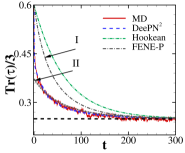
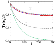
Figure 1: Quasi-equilibrium relaxation process of a dumbbell suspension obtained from direct MD simulation, the present DeePN², canonical Hookean and FENE-P model. Left: Encoder function $g(r)$. Middle: Evolution of $\bm{\tau}_{\rm p}$. Right: Evolution of $\mathbf{c}_{1}=\left\langle\mathbf{r}\mathbf{r}^{T}\right\rangle$. Two parameter sets of the FENE-P model are examined: (I) the initial conditions of both $\mathbf{c}_{1}$ and $\bm{\tau}_{\rm p}$ are consistent with MD. (II) the initial and final conditions of $\mathbf{c}_{1}$ are consistent with MD. The Hookean model parameters are set following (I).

Fig. 1 shows the encoder functions $g(r)$ with $r_{0}=2.4$, $k_{s}=0.1$. To validate the DeePN² model, we consider a quasi-equilibrium dynamics of the polymer solution with $k_{B}T=0.25$, while the initial polymer configuration is taken from the equilibrium state with $k_{B}T=0.6$. The relaxation process is simulated using both MD and DeepN². Fig. 1 shows the evolution of the trace of $\mathbf{c}_{1}$ and $\bm{\tau}_{\rm p}$. The predictions from DeePN² agree well with the MD results. In contrast, the predictions from Hookean and FENE-P model show apparent deviations.

Next, we consider the non-equilibrium process of a reverse Poiseuille flow (RPF) in a domain $[0,40]\times[0,80]\times[0,40]$ (reduced unit), with periodic boundary condition imposed in each direction. Starting from $t=0$, an external field $\mathbf{f}_{\rm ext}=(f_{b},0,0)$ is applied in the region $y<40$ and an opposite field $\mathbf{f}_{\rm ext}=(-f_{b},0,0)$ is applied in the region $y>40$. Fig. 2 shows the instantaneous velocity profiles with $r_{0}=3.8$ and $f_{b}=0.02$. The predictions from DeePN² agree well with MD while FENE-P yields apparent deviations. For the velocity evolution at $y=6$ and $y=14$, the predictions from the Hookean and FENE-P models show pronounced overestimations on both the magnitude and duration of the oscillation behavior. Such limitations of the FENE-P model have already been noted in Ref. Laso and Öttinger (1993). From the microscopic perspective, the discrepancy arises from the mean field approximation, $\bm{\tau}_{\rm p}\approx\mathbf{c}/(1-\operatorname{Tr}(\mathbf{c})/r_{0}^{2})$. Such an approximation cannot capture the nonlinear response when individual polymer bond length approaches $r_{0}$. In contrast, DeePN² can capture such micro-scale “bond length dispersion” via the additional macro-scale nonlinear conformation tensors $\mathbf{c}_{2},\cdots,\mathbf{c}_{n}$.

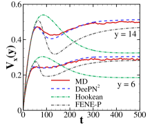
Figure 2: Evolution of the reverse Poiseuille flow of a dumbbell suspension obtained from MD and various models. Left: velocity profiles at $t=20,60,220$. Right: velocity evolution at $y=6$ and $y=14$. The parameters of the Hookean and FENE-P model are chosen such that the equilibrium bond length matches the MD results.

Shown in Fig. 3(a) is the evolution of $\mathbf{c}_{1}$ at $y=6$. The DeePN² faithfully predicts the responses of the polymer configurations under the external flow field. The instantaneous $\bm{\tau}_{\rm p}$ is also accurately predicted by the conformation tensors, as shown in Fig. 3(b-c). The responses can also be examined by the shear-rate-dependent viscosity. As shown in Fig. 3(d), predictions by DeePN² agree well with the MD results. In contrast, the FENE-P model yields apparent deviations.

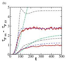
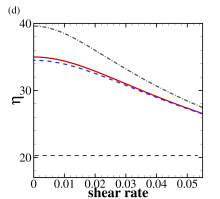
Figure 3: The micro-macro correspondence during the evolution of the reverse Poiseuille flow of the dumbbell suspension presented in Fig. 2 with the same line scheme. (a) evolution of $\mathbf{c}_{1}$ at $y=6$. (b-c) Normal stress difference ${\bm{\tau}_{\rm p}}_{xx}-{\bm{\tau}_{\rm p}}_{yy}$ and shear stress ${\bm{\tau}_{\rm p}}_{xy}$ at $y=6$ (upper lines) and $y=14$ (lower lines). (d) Shear-rate-dependent viscosity. The predictions by Hookean model show large deviations from the MD results, and not shown in (a), (c), (d) for visualization purpose.

Besides the first-principle-based stress model and dynamic closure, another distinctive feature of the DeePN² model is the generalized objective tensor derivative $\mathcal{D}\mathbf{c}_{i}/\mathcal{D}t$:

$$\frac{\mathcal{D}\mathbf{c}_{i}}{\mathcal{D}t}=\overset{\triangledown}{\mathbf{c}}_{i}-\bm{\kappa}:\left[\sum_{k=1}^{6}\mathbf{E}_{1,i}^{(k)}(\mathbf{c}_{1},\cdots,\mathbf{c}_{n})\otimes\mathbf{E}_{2,i}^{(k)}(\mathbf{c}_{1},\cdots,\mathbf{c}_{n})\right],$$ (15)

where $\overset{\triangledown}{\mathbf{c}}_{i}$ is the standard upper-convected derivative and the second term arises from the source term $\left\langle\mathbf{r}\nabla_{\mathbf{r}}g(r)^{2}\otimes\mathbf{r}\mathbf{r}^{T}\right\rangle$ in Eq. (7). Therefore, the second term of $\mathcal{D}\mathbf{c}_{i}/\mathcal{D}t$ is embedded with the nonlinear response to external field $\bm{\kappa}$, inherited from the encoder $g_{i}(r)$. As a numerical test, we use the present model to simulate the RPF, where $\mathcal{D}\mathbf{c}_{i}/\mathcal{D}t$ is chosen to be the upper-convected derivative $\overset{\triangledown}{\mathbf{c}}_{i}$ and other modeling terms remain the same. Fig. 4 shows the evolution of the velocities and $\mathbf{c}_{1}$. By ignoring the second term in Eq. (15), the predictions show apparent deviations from the MD results. This indicates that the empirical choices of the objective tensor derivative are not accurate. To achieve the desired accuracy, these derivatives have to retain some information from the specific conformation tensor.

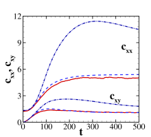
Figure 4: The effectiveness of the objective tensor derivative constructed by (15). The additional source term plays a vital role in the accurate modeling of the fluid systems. The model that uses the canonical upper-convected derivative shows apparent deviations from the MD results for the evolution of the velocities (left) and $\mathbf{c}_{1}$ (right) at $y=6$.

IV Discussion

The present DeePN² directly learns the stress model and constitutive dynamics from the microscale simulation data and avoids dealing with the high-dimensional microscale configuration density function $\rho(\mathbf{r},t)$. A main observation is that the explicit knowledge of $\rho(\mathbf{r},t)$ is a sufficient, but not a necessary condition for constructing the full constitutive equation. We note that DeePN² differs from the previous moment-closure studies Warner (1972, 1971); Armstrong (1974) based on empirical approximations of $\rho(\mathbf{r},t)$. In these semi-analytical studies Warner (1972, 1971); Armstrong (1974), the steady-state FK solution $\rho_{s}(\mathbf{r})$ of a dumbbell is approximated by series expansion, yielding the stress-strain relationship only for equilibrium Bird et al. (1987). In Ref. Du et al. (2005); Yu et al. (2005); Hyon et al. (2008), a set of high-order moments are proposed to capture the peak regime of the $\rho(\mathbf{r},t)$, yielding good predictions for the two-dimensional dumbbell system. However, it is not straightforward to generalize such approximations for complex systems due to the lack of general relationship between these moments and the stress tensor $\bm{\tau}_{\rm p}$. On the other hand, the conformation tensors constructed in the present DeePN² are not the standard moments for the approximation of $\rho(\mathbf{r},t)$; they are directly learnt from the micro-scale samples that best capture the dynamics of $\bm{\tau}_{\rm p}$, rather than recover the high-dimensional $\rho(\mathbf{r},t)$. As a numerical example, we employ DeePN² to a three-bead suspension with intramolecular interactions governed by both the bond and angle potentials, see Appendix. Generalization of the learning framework for complex polymer fluids will be conducted and presented in the following studies.

V Summary

In this study, we presented a machine learning-based approach for constructing hydrodynamic models for polymer fluids, DeePN², directly from the micro-scale descriptions. While this is only the first step in a long program, the results we obtained have already demonstrated the potential of such an approach for achieving accuracy and efficiency at the same time. The construction is based on an underlying micro-scale model. It respects the symmetries of the underlying physical system. It is end-to-end, and requires little ad hoc human intervention. Contrary to conventional wisdom on machine learning models, the model obtained here is quite interpretable, and in fact shows quite some physical insight. It has already demonstrated much better accuracy than existing hydrodynamic models in several tests.

Different from the common ML-based approaches for learning the reduced dynamics of complex systems, the present approach does not require the time-series samples and provides a generalized form of the objective tensor derivative with clear micro-scale interpretation. This enables us to avoid the heuristic choices on the objective tensor derivative and the “black-box” representations by the numerical evaluation of the time-derivatives. These unique features are well-suited for the multi-scale fluid systems where accurate time-series samples from the micro-scale simulations are often limited. While we focused on polymer solutions, the new form of the objective tensor derivative and the present learning framework are quite general and can be adapted to other systems of complex fluids and soft matter.

It should also be noted that what we discussed is only a first step towards constructing accurate and robust hydrodynamic models for non-Newtonian fluids. Admittedly, dumbbell suspensions are polymer models with simplified intramolecular potential and viscoelasticity, applications to more realistic micro-scale models will be carried out in future work. Among the other issues that remain to be addressed, let us mention coupling the training process with the adaptive selection of the training data as was done in MD Zhang et al. (2019), the automatic choice of the model complexity (e.g. the choice of $n$), the improvement of the underlying micro-scale model Lei et al. (2016), and the enhancement of the micro-scale sampling efficiency. While some of these will take time, there is no doubt that machine learning, used in the right way, can help us to tackle the long-standing problem of developing truly reliable hydrodynamic models for complex fluids.

Appendix A Rotational symmetry of the model ansatz and the DNN representation

In this section, we show that both the modeling ansatz and the DNN representation of the DeePN² model satisfy the rotational invariance condition.

A.1 Rotational invariance from the continuum and microscopic perspective

Let us consider a symmetric tensor $\mathbf{c}\in\mathbb{R}^{3\times 3}$ in two different coordinate frames. Frame $1$ is a static inertial frame. We let $\tilde{\mathbf{x}}$, $\tilde{\mathbf{v}}:=\tilde{\mathbf{v}}(\tilde{\mathbf{x}},t)$, $\tilde{\mathbf{c}}:=\tilde{\mathbf{c}}(\tilde{\mathbf{x}},t)$, the position, velocity and $\mathbf{c}$ in frame $1$. Framework $2$ is a rotated frame which is related to frame $1$ by a unitary matrix $\mathbf{Q}(t)$. We denote $\mathbf{x}$, $\mathbf{v}(\mathbf{x},t)$, $\mathbf{c}(\mathbf{x},t)$ the position, velocity and $\mathbf{c}$ in frame $2$. Accordingly, $\mathbf{x}$, $\mathbf{c}$ and $\mathbf{v}$ follows the transformation rule

$$\begin{split}&\tilde{\mathbf{x}}=\mathbf{Q}\mathbf{x}\\ &\tilde{\mathbf{v}}=\mathbf{Q}\mathbf{v}(\mathbf{x},t)+\dot{\mathbf{Q}}\mathbf{Q}^{T}\tilde{\mathbf{x}}\\ &\tilde{\mathbf{c}}=\mathbf{Q}\mathbf{c}(\mathbf{x},t)\mathbf{Q}^{T}.\end{split}$$ (16)

To construct the dynamics of $\mathbf{c}$, we need to choose an objective derivative $\displaystyle\frac{\mathcal{D}\mathbf{c}}{\mathcal{D}t}$ which retains proper rotational symmetry, i.e.,

$$\frac{\mathcal{D}\tilde{\mathbf{c}}}{\mathcal{D}t}\big{|}_{\rm frame1}=\mathbf{Q}(t)\frac{\mathcal{D}\mathbf{c}}{\mathcal{D}t}\big{|}_{\rm frame2}\mathbf{Q}(t)^{T}.$$ (17)

For introduction, we choose $\mathcal{D}/\mathcal{D}t$ to be the material derivative of the vector form, i.e., $\displaystyle\frac{\rm d}{\rm dt}:=\frac{\partial}{\partial t}+\mathbf{v}\cdot\nabla$. Accordingly, Eq. (17) cannot be satisfied, since

$$\begin{split}\frac{\mathcal{D}\tilde{\mathbf{c}}}{\mathcal{D}t}\big{|}_{\rm frame1}&=\dot{\mathbf{Q}}\mathbf{c}\mathbf{Q}^{T}+\mathbf{Q}\mathbf{c}\dot{\mathbf{Q}}^{T}+\mathbf{Q}\frac{\mathop{}\!\mathrm{d}\mathbf{c}}{\mathop{}\!\mathrm{d}t}\big{|}_{\rm frame~{}1}\mathbf{Q}^{T}\\ &=\dot{\mathbf{Q}}\mathbf{c}\mathbf{Q}^{T}+\mathbf{Q}\mathbf{c}\dot{\mathbf{Q}}^{T}+\mathbf{Q}\frac{\mathcal{D}\mathbf{c}}{\mathcal{D}t}\big{|}_{\rm frame~{}2}\mathbf{Q}^{T}.\end{split}$$ (18)

Compared with Eq. (17), two additional terms appear in the last equation. The second identity follows from

$$\begin{split}\frac{\rm d\mathbf{c}}{\rm dt}\big{|}_{\rm frame~{}1}&=\frac{\partial\mathbf{c}(\mathbf{Q}^{T}\tilde{\mathbf{x}},t)}{\partial t}+\tilde{\mathbf{v}}\cdot\nabla_{\tilde{\mathbf{x}}}\mathbf{c}(\mathbf{Q}^{T}\tilde{\mathbf{x}},t)\\ &=\frac{\partial\mathbf{c}(\mathbf{x},t)}{\partial t}+\left(\dot{\mathbf{Q}}^{T}\tilde{\mathbf{x}}\cdot\nabla_{\mathbf{x}}\right)\mathbf{c}+\left(\mathbf{Q}\mathbf{v}(\mathbf{x},t)+\dot{\mathbf{Q}}\mathbf{x}\right)\cdot\nabla_{\tilde{\mathbf{x}}}\mathbf{c}\\ &=\frac{\partial\mathbf{c}(\mathbf{x},t)}{\partial t}+\mathbf{v}(\mathbf{x},t)\cdot\nabla_{\mathbf{x}}\mathbf{c}\\ &=\frac{\rm d\mathbf{c}}{\rm dt}\big{|}_{\rm frame~{}2}.\end{split}$$

Alternatively, if we choose $\mathcal{D}/\mathcal{D}t$ to be the objective tensor derivatives coupled with $\bm{\kappa}:=\left(\nabla\mathbf{v}\right)^{T}$, e.g., the upper-convected $\overset{\triangledown}{\mathbf{c}}=\frac{\rm d\mathbf{c}}{\rm dt}-\bm{\kappa}\mathbf{c}-\mathbf{c}\bm{\kappa}^{T}$, covariant derivative $\overset{\vartriangle}{\mathbf{c}}=\frac{\rm d\mathbf{c}}{\rm dt}+\bm{\kappa}^{T}\mathbf{c}+\mathbf{c}\bm{\kappa}$, the Jaumann derivative $\overset{\circ}{\mathbf{c}}=\frac{1}{2}(\overset{\triangledown}{\mathbf{c}}+\overset{\vartriangle}{\mathbf{c}})$, Eq. (17) is satisfied. For example,

$$\begin{split}\overset{\triangledown}{\mathbf{c}}\big{|}_{\rm frame~{}1}&=\dot{\mathbf{Q}}\mathbf{c}\mathbf{Q}^{T}+\mathbf{Q}\mathbf{c}\dot{\mathbf{Q}}^{T}+\mathbf{Q}\frac{\rm d\mathbf{c}}{\rm dt}\big{|}_{\rm frame~{}2}\mathbf{Q}^{T}\\ &-(\mathbf{Q}\bm{\kappa}\mathbf{Q}^{T}+\dot{\mathbf{Q}}\mathbf{Q}^{T})\mathbf{Q}\mathbf{c}\mathbf{Q}^{T}-\mathbf{Q}\mathbf{c}\mathbf{Q}^{T}(\mathbf{Q}\bm{\kappa}^{T}\mathbf{Q}^{T}+\mathbf{Q}\dot{\mathbf{Q}}^{T})\\ &=\mathbf{Q}\frac{\rm d\mathbf{c}}{\rm dt}\big{|}_{\rm frame~{}2}\mathbf{Q}^{T}-\mathbf{Q}\bm{\kappa}\mathbf{c}\mathbf{Q}^{T}-\mathbf{Q}^{T}\mathbf{c}\bm{\kappa}^{T}\mathbf{Q}\\ &=\mathbf{Q}\overset{\triangledown}{\mathbf{c}}\big{|}_{\rm frame~{}2}\mathbf{Q}^{T}.\end{split}$$

On the other hand, this analysis does not provide us concrete guidance to construct $\frac{\mathcal{D}\mathbf{c}}{\mathcal{D}t}$, since multiple choices such as $\overset{\triangledown}{\mathbf{c}}$, $\overset{\vartriangle}{\mathbf{c}}$ and $\overset{\circ}{\mathbf{c}}$ all satisfy Eq. (17). To address this issue, we look for a micro-scale perspective based on the Fokker-Planck equation to understand the rotational invariance and construct $\frac{\mathcal{D}\mathbf{c}}{\mathcal{D}t}$.

Let us consider the Fokker-Planck equation of a dumb-bell polymer with end-end vector $\mathbf{r}$ coupled with flow field $\mathbf{v}$. By ignoring the external field, the evolution of the density $\rho(\mathbf{r},t)$ is governed by

$$\frac{\partial\rho(\mathbf{r},t)}{\partial t}=-\nabla\cdot\left[(\bm{\kappa}\cdot\mathbf{r})\rho-\frac{2k_{B}T}{\gamma}\nabla\rho-\frac{2}{\gamma}\nabla V_{\rm b}\rho\right],$$ (19)

where $\gamma$ is the friction coefficient of the solvent, $V_{\rm b}(r)$ is the intra-molecule potential energy.

Proposition A.1.

Eq. (19) retains rotational invariance under the transformation by Eq. (16), i.e.

$$\tilde{\rho}:=\rho\left(\tilde{\mathbf{r}},t\right)\big{|}_{\rm frame~{}1}\equiv\rho\left(\mathbf{r},t\right)\big{|}_{\rm frame~{}2}.$$

Proof.

$$\begin{split}&\frac{\partial\tilde{\rho}}{\partial t}+\nabla_{\tilde{\mathbf{r}}}\cdot\left(\left(\tilde{\bm{\kappa}}\cdot\tilde{\mathbf{r}}\right)\tilde{\rho}\right)\big{|}_{\rm frame~{}1}\\ &=\frac{\partial\rho}{\partial t}+\dot{\mathbf{Q}}^{T}\tilde{\mathbf{r}}\cdot\nabla_{\mathbf{r}}\rho+\nabla_{\tilde{\mathbf{r}}}\cdot\left(\left(\mathbf{Q}\bm{\kappa}\mathbf{Q}^{T}+\dot{\mathbf{Q}}\mathbf{Q}^{T}\right)\cdot\mathbf{Q}\rho\right)\\ &=\frac{\partial\rho}{\partial t}+\dot{\mathbf{Q}}^{T}\mathbf{Q}\mathbf{r}\cdot\nabla_{\mathbf{r}}\rho+\nabla_{\mathbf{r}}\cdot\left(\bm{\kappa}\cdot\mathbf{r}\rho\right)+\nabla_{\mathbf{r}}\cdot\left(\mathbf{Q}^{T}\dot{\mathbf{Q}}\mathbf{r}\rho\right)\\ &\equiv\frac{\partial\rho}{\partial t}+\nabla_{\mathbf{r}}\cdot\left(\bm{\kappa}\cdot\mathbf{r}\rho\right)\big{|}_{\rm frame~{}2}.\end{split}$$

where we have used the fact that $\dot{\mathbf{Q}}^{T}\mathbf{Q}$ is anti-symmetric. In addition, it is straightforward to show that the terms $\nabla^{2}\rho$ and $\nabla\cdot\nabla V_{\rm b}(r)$ are invariant. Therefore we have (A.1). ∎

Accordingly, if we define $\mathbf{c}$ to be the mean value of a second-order tensor $\mathbf{B}(\mathbf{r}):\mathbb{R}^{3}\to\mathbb{R}^{3\times 3}$, the dynamics follows

$$\frac{\rm d}{\rm dt}\left\langle\mathbf{B}(\mathbf{r})\right\rangle=\bm{\kappa}:\left\langle\mathbf{r}\nabla_{\mathbf{r}}\otimes\mathbf{B}\right\rangle+\frac{2k_{B}T}{\gamma}\left\langle\nabla^{2}\mathbf{B}\right\rangle+\frac{2}{\gamma}\left\langle\nabla V_{\rm b}\cdot\nabla\mathbf{B}\right\rangle.$$ (20)

Proposition A.2.

If $\mathbf{B}(r)$ obeys rotational symmetry $\tilde{\mathbf{B}}:=\mathbf{B}(\mathbf{Q}^{T}r)=\mathbf{Q}\mathbf{B}\mathbf{Q}^{T}$, then so does (20).

Proof.

Using Eq. (18), the individual terms in frame $1$ follow

$$\frac{\rm d}{\rm dt}\left\langle\tilde{\mathbf{B}}\right\rangle\big{|}_{\rm frame~{}1}=\dot{\mathbf{Q}}\left\langle\mathbf{B}\right\rangle\mathbf{Q}^{T}+\mathbf{Q}\left\langle\mathbf{B}\right\rangle\dot{\mathbf{Q}}^{T}+\mathbf{Q}\frac{\rm d}{\rm dt}\left\langle\mathbf{B}\right\rangle\big{|}_{\rm frame~{}2}\dot{\mathbf{Q}}^{T}.$$ (21)

Note that

$$\begin{split}&\tilde{\bm{\kappa}}:\left\langle\tilde{\mathbf{r}}\nabla_{\tilde{\mathbf{r}}}\otimes\tilde{\mathbf{B}}\right\rangle\big{|}_{\rm frame1}\\ &=\left[\left(\mathbf{Q}\bm{\kappa}\mathbf{Q}^{T}+\dot{\mathbf{Q}}\mathbf{Q}^{T}\right)\cdot\mathbf{Q}\mathbf{r}\right]\cdot\mathbf{Q}\nabla_{\mathbf{r}}\left(\mathbf{Q}\mathbf{B}\mathbf{Q}^{T}\right)\\ &=\left(\bm{\kappa}\cdot\mathbf{r}\right)\cdot\nabla_{\mathbf{r}}\left(\mathbf{Q}\mathbf{B}\mathbf{Q}^{T}\right)+(\mathbf{Q}^{T}\dot{\mathbf{Q}}\mathbf{r})\cdot\nabla_{\mathbf{r}}\left(\mathbf{Q}\mathbf{B}\mathbf{Q}^{T}\right)\\ &=\mathbf{Q}(\bm{\kappa}\cdot\mathbf{r})\cdot\nabla_{\mathbf{r}}\mathbf{B}\mathbf{Q}^{T}+\mathbf{Q}\left(\mathbf{Q}^{T}\dot{\mathbf{Q}}\mathbf{B}+\mathbf{B}\dot{\mathbf{Q}}^{T}\mathbf{Q}\right)\mathbf{Q}^{T},\end{split}$$ (22)

where we have used the relation

$$\left(\mathbf{A}\mathbf{r}\right)\cdot\nabla\mathbf{B}=\mathbf{A}\mathbf{B}+\mathbf{B}\mathbf{A}^{T},$$ (23)

if $\mathbf{B}$ is a rotational symmetric tensor and $\mathbf{A}=\mathbf{Q}^{T}\dot{\mathbf{Q}}$ is an anti-symmetric tensor.

By Eq. (21) and (22), we see that

$$\frac{\rm d}{\rm dt}\left\langle\tilde{\mathbf{B}}\right\rangle\big{|}_{\rm frame~{}1}-\tilde{\bm{\kappa}}:\left\langle\tilde{\mathbf{r}}\nabla_{\tilde{\mathbf{r}}}\otimes\tilde{\mathbf{B}}\right\rangle\big{|}_{\rm frame~{}1}\equiv\mathbf{Q}\left[\frac{\rm d}{\rm dt}\left\langle\mathbf{B}\right\rangle\big{|}_{\rm frame~{}2}-\bm{\kappa}:\left\langle\mathbf{r}\nabla_{\mathbf{r}}\otimes\mathbf{B}\right\rangle\big{|}_{\rm frame~{}2}\right]\mathbf{Q}^{T}.$$

The rotational symmetry of the other terms follows similarly. ∎

The above analysis shows that, from the perspective of the Fokker-Planck equation, the evolution dynamics retains the rotational symmetry. In particular, the term $\frac{\rm d}{\rm dt}\left\langle\tilde{\mathbf{B}}\right\rangle-\tilde{\bm{\kappa}}:\left\langle\tilde{\mathbf{r}}\nabla_{\tilde{\mathbf{r}}}\otimes\tilde{\mathbf{B}}\right\rangle$ provides a microscopic perspective for understanding the objective tensor derivative $\frac{\mathcal{D}\mathbf{B}}{\mathcal{D}t}$, which we use to construct the DNN representation of the constitutive models.

A.2 DNN representation

Next we establish a micro-macro correspondence via a set of encoder $\left\{g_{i}(r)\right\}_{i=1}^{n}$ (see Proposition A.4 for details) and, accordingly, a set of micro-scale tensor $\mathbf{B}_{i}$ and $\mathbf{c}_{i}$, i.e.,

$$\mathbf{B}_{i}(\mathbf{r})=\left(g_{i}(r)\mathbf{r}\right)\left(g_{i}(r)\mathbf{r}\right)^{T},\quad\mathbf{c}_{i}=\left\langle\mathbf{B}_{i}\right\rangle.$$

We will use $\left\{\mathbf{c}_{i}\right\}_{i=1}^{n}$ to construct the evolution dynamics (20) via some proper DNN structure which retains the rotational invariance. In particular, we consider the fourth-order tensor $\left\langle\mathbf{r}\nabla_{\mathbf{r}}\otimes\mathbf{B}\right\rangle$ and show that the following DNN representation (see also Eq. (12) in main text) ensures the rotational symmetry of $\frac{\mathcal{D}\mathbf{B}}{\mathcal{D}t}$. For simplicity, the subscript $i$ is ignored and we use $\mathbf{c}$ to denote the set of conformation tensor $\left\{\mathbf{c}_{i}\right\}_{i=1}^{n}$.

Proposition A.3.

The following ansatz of $\left\langle\mathbf{r}\nabla_{\mathbf{r}}\otimes\mathbf{B}\right\rangle$ ensures that the dynamic of evolution of $\mathbf{c}$ retains rotational invariance.

$$\boxed{\left\langle\mathbf{r}\nabla_{\mathbf{r}}\otimes\mathbf{B}\right\rangle=\left\langle g(r)^{2}\mathbf{r}\nabla_{\mathbf{r}}\otimes{\color[rgb]{0,0,0}{\mathbf{r}}}{\color[rgb]{0,0,0}{\mathbf{r}^{T}}}\right\rangle+\sum_{i=1}^{6}\mathbf{E}_{1}^{(i)}(\mathbf{c})\otimes\mathbf{E}_{2}^{(i)}(\mathbf{c})}$$

where $\mathbf{E}_{1}$ and $\mathbf{E}_{2}$ satisfy

$$\tilde{\mathbf{E}}_{1}:=\mathbf{E}_{1}(\tilde{\mathbf{c}})=\mathbf{Q}\mathbf{E}_{1}\mathbf{Q}^{T}\quad\tilde{\mathbf{E}}_{2}:=\mathbf{E}_{2}(\tilde{\mathbf{c}})=\mathbf{Q}\mathbf{E}_{2}\mathbf{Q}^{T}.$$

Proof.

Without loss of generality, we represent the fourth order tensor by the following two bases

$$\begin{split}&\mathbf{F}_{1}(\mathbf{c})\otimes\mathbf{F}_{2}(\mathbf{c})\otimes\mathbf{F}_{3}(\mathbf{c})+\mathbf{F}_{1}(\mathbf{c})\otimes\left(\mathbf{F}_{2}(\mathbf{c})\otimes\mathbf{F}_{3}(\mathbf{c})\right)^{T_{\{2,3\}}}\\ &\mathbf{E}_{1}(\mathbf{c})\otimes\mathbf{E}_{2}(\mathbf{c})\\ &\mathbf{F}_{1},\mathbf{F}_{3}\in\mathbb{R}^{3},\mathbf{F}_{2}\in\mathbb{R}^{3\times 3},\mathbf{E}_{1},\mathbf{E}_{2}\in\mathbb{R}^{3\times 3},\end{split}$$

where the super-script $T_{\{2,3\}}$ represent the transpose between the 2nd and 3rd indices; also $\mathbf{F}_{1}$, $\mathbf{F}_{2}$, $\mathbf{F}_{3}$, $\mathbf{E}_{1}$ and $\mathbf{E}_{2}$ satisfy the symmetry conditions

$$\begin{split}&\mathbf{F}_{1}(\tilde{\mathbf{c}})=\mathbf{Q}\mathbf{F}_{1}\quad\mathbf{F}_{3}(\tilde{\mathbf{c}})=\mathbf{Q}\mathbf{F}_{3}\\ &\mathbf{E}_{1}(\tilde{\mathbf{c}})=\mathbf{Q}\mathbf{E}_{1}\mathbf{Q}^{T}\quad\mathbf{E}_{2}(\tilde{\mathbf{c}})=\mathbf{Q}\mathbf{E}_{2}\mathbf{Q}^{T}\quad\mathbf{F}_{2}(\tilde{\mathbf{c}})=\mathbf{Q}\mathbf{F}_{2}\mathbf{Q}^{T}.\end{split}$$

For the term $\mathbf{E}_{1}(\mathbf{c})\otimes\mathbf{E}_{2}(\mathbf{c})$, we have

$$\bm{\kappa}:\mathbf{E}_{1}(\mathbf{c})\otimes\mathbf{E}_{2}(\mathbf{c})\big{|}_{\rm frame2}=\operatorname{Tr}(\bm{\kappa}\mathbf{E}_{1})\mathbf{E}_{2}$$

and

$$\begin{split}&\tilde{\bm{\kappa}}:\tilde{\mathbf{E}}_{1}(\mathbf{c})\otimes\tilde{\mathbf{E}}_{2}(\mathbf{c})\big{|}_{\rm frame1}\\ &=\left(\mathbf{Q}\bm{\kappa}\mathbf{Q}^{T}+\dot{\mathbf{Q}}\mathbf{Q}^{T}\right):\left(\mathbf{Q}\mathbf{E}_{1}\mathbf{Q}^{T}\otimes\tilde{\mathbf{E}}_{2}\right)\\ &=\operatorname{Tr}(\bm{\kappa}\mathbf{E}_{1})\tilde{\mathbf{E}}_{2}+\operatorname{Tr}(\dot{\mathbf{Q}}\mathbf{Q}^{T}\mathbf{Q}\mathbf{E}_{1}\mathbf{Q}^{T})\tilde{\mathbf{E}}_{2}\\ &=\operatorname{Tr}(\bm{\kappa}\mathbf{E}_{1})\tilde{\mathbf{E}}_{2}\\ &\equiv\mathbf{Q}\left(\bm{\kappa}:\mathbf{E}_{1}(\mathbf{c})\otimes\mathbf{E}_{2}(\mathbf{c})\big{|}_{\rm frame2}\right)\mathbf{Q}^{T},\end{split}$$ (24)

where we have used $\operatorname{Tr}(\dot{\mathbf{Q}}\mathbf{Q}^{T})\equiv 0$.

For the term $\mathbf{F}_{1}(\mathbf{c})\otimes\mathbf{F}_{2}(\mathbf{c})\otimes\mathbf{F}_{3}(\mathbf{c})+\mathbf{F}_{1}(\mathbf{c})\otimes\left(\mathbf{F}_{2}(\mathbf{c})\otimes\mathbf{F}_{3}(\mathbf{c})\right)^{T_{\{2,3\}}}$, we have

$$\bm{\kappa}:\mathbf{F}_{1}(\mathbf{c})\otimes\mathbf{F}_{2}(\mathbf{c})\otimes\mathbf{F}_{3}(\mathbf{c})\big{|}_{\rm frame2}=\mathbf{F}_{2}^{T}\bm{\kappa}\mathbf{F}_{1}\mathbf{F}_{3}^{T}$$

and

$$\tilde{\bm{\kappa}}:\tilde{\mathbf{F}}_{1}(\mathbf{c})\otimes\tilde{\mathbf{F}}_{2}(\mathbf{c})\otimes\tilde{\mathbf{F}}_{3}(\mathbf{c})\big{|}_{\rm frame1}=\mathbf{Q}\mathbf{F}_{2}^{T}\bm{\kappa}\mathbf{F}_{1}\mathbf{F}_{3}^{T}\mathbf{Q}^{T}+\mathbf{Q}\mathbf{F}_{2}^{T}\mathbf{Q}^{T}\dot{\mathbf{Q}}\mathbf{F}_{1}\mathbf{F}_{3}^{T}\mathbf{Q}^{T}.$$

On the other hand, note that

$$\frac{\mathop{}\!\mathrm{d}\tilde{\mathbf{B}}}{\mathop{}\!\mathrm{d}t}\big{|}_{\rm frame1}=\dot{\mathbf{Q}}\mathbf{B}\mathbf{Q}^{T}+\mathbf{Q}\mathbf{B}\dot{\mathbf{Q}}^{T}+\mathbf{Q}\frac{\mathop{}\!\mathrm{d}\mathbf{B}}{\mathop{}\!\mathrm{d}t}\big{|}_{\rm frame~{}2}\mathbf{Q}^{T}.$$ (25)

To ensure the rotational symmetry of $\frac{\mathcal{D}\mathbf{B}}{\mathcal{D}t}$, we have

$$\mathbf{F}_{2}\equiv\mathbf{I},\sum_{i=1}^{K_{1}}\mathbf{F}_{1}^{(i)}\otimes\mathbf{I}\otimes\mathbf{F}_{3}^{(i)}=\left\langle g(r)\mathbf{r}\otimes\mathbf{I}\otimes g(r)\mathbf{r}\right\rangle.$$ (26)

Hence, we have

$$\begin{split}&\frac{\rm d}{\rm dt}\tilde{\mathbf{c}}-\tilde{\bm{\kappa}}:\left(\sum_{i=1}^{K_{1}}\tilde{\mathbf{F}}_{1}^{(i)}\otimes\tilde{\mathbf{F}}_{2}^{(i)}\otimes\tilde{\mathbf{F}}_{3}^{(i)}+\tilde{\mathbf{F}}_{1}^{(i)}\otimes\left(\tilde{\mathbf{F}}_{2}^{(i)}\otimes\tilde{\mathbf{F}}_{3}^{(i)}\right)^{T_{\{2,3\}}}\right)\big{|}_{\rm frame1}\\ &\equiv\mathbf{Q}\left[\frac{\rm d}{\rm dt}\mathbf{c}-\bm{\kappa}:\left(\sum_{i=1}^{K_{1}}\mathbf{F}_{1}^{(i)}\otimes\mathbf{F}_{2}^{(i)}\otimes\mathbf{F}_{3}^{(i)}+\mathbf{F}_{1}^{(i)}\otimes\left(\mathbf{F}_{2}^{(i)}\otimes\mathbf{F}_{3}^{(i)}\right)^{T_{\{2,3\}}}\right)\big{|}_{\rm frame2}\right]\mathbf{Q}^{T}.\end{split}$$ (27)

Furthermore, using Eq. (26), we obtain

$$\sum_{i=1}^{K_{1}}\mathbf{F}_{1}^{(i)}\otimes\mathbf{F}_{2}^{(i)}\otimes\mathbf{F}_{3}^{(i)}+\mathbf{F}_{1}^{(i)}\otimes\left(\mathbf{F}_{2}^{(i)}\otimes\mathbf{F}_{3}^{(i)}\right)^{T_{\{2,3\}}}=\left\langle g(r)^{2}\mathbf{r}\nabla_{\mathbf{r}}\otimes{\color[rgb]{0,0,0}{\mathbf{r}}}{\color[rgb]{0,0,0}{\mathbf{r}^{T}}}\right\rangle.$$ (28)

Accordingly, the remaining part of $\left\langle\mathbf{r}\nabla_{\mathbf{r}}\otimes\mathbf{B}\right\rangle$ is expanded by

$$\left\langle\mathbf{r}\nabla_{\color[rgb]{0,0,0}{\mathbf{r}}}g(r)^{2}\otimes{\mathbf{r}}\mathbf{r}^{T}\right\rangle=\sum_{i=1}^{K_{2}}\mathbf{E}_{1}^{(i)}(\mathbf{c})\otimes\mathbf{E}_{2}^{(i)}(\mathbf{c}).$$ (29)

where $K_{2}=6$ due to the tensor index symmetry of $1$ and $2$, as well as $3$ and $4$.

Combining Eq. (27), (28) and (29), we conclude that the decomposition

$$\boxed{\left\langle\mathbf{r}\nabla_{\mathbf{r}}\otimes\mathbf{B}\right\rangle=\left\langle g(r)^{2}\mathbf{r}\nabla_{\mathbf{r}}\otimes{\color[rgb]{0,0,0}{\mathbf{r}}}{\color[rgb]{0,0,0}{\mathbf{r}^{T}}}\right\rangle+\sum_{i=1}^{6}\mathbf{E}_{1}^{(i)}(\mathbf{c})\otimes\mathbf{E}_{2}^{(i)}(\mathbf{c})}$$

ensures the rotational invariance in the dynamic equation of $\mathbf{c}$. ∎

Finally, we show that the encoder $\mathbf{f}_{i}(\mathbf{r})$ takes the form $g_{i}(|\mathbf{r}|)\mathbf{r}$ (see also Eq. (10) in the main text).

Proposition A.4.

If $\mathbf{f}(\mathbf{r}):\mathbb{R}^{3}\to\mathbb{R}^{3}$ satisfies

$$\mathbf{f}(\mathbf{Q}\mathbf{r})=\mathbf{Q}\mathbf{f}(\mathbf{r})$$

for an arbitrary unitary matrix $\mathbf{Q}\in\mathbb{R}^{3}$, then $\mathbf{f}(\mathbf{r})$ must take the form $\mathbf{f}(\mathbf{r})=g(r)\mathbf{r}$, where $g(r):\mathbb{R}\to\mathbb{R}$ is a scalar function and $r=|\mathbf{r}|$.

Proof.

Let $\mathbf{e}_{1}$, $\mathbf{e}_{2}$ and $\mathbf{e}_{3}$ the basis vectors of the cartesian coordinate space. In particular, we consider $\mathbf{r}=r\mathbf{e}_{1}$ and denote $\mathbf{f}(\mathbf{r})$ by $\left(f_{1}(\mathbf{r}),f_{2}(\mathbf{r}),f_{3}(\mathbf{r})\right)$. By choosing $\mathbf{Q}$ to be of the form

$$\mathbf{Q}=\begin{pmatrix}0&\cos\theta&\sin\theta\\ 1&0&0\\ 0&-\sin\theta&\cos\theta\end{pmatrix},$$

we have

$$\mathbf{f}(\mathbf{Q}\mathbf{r})=\begin{pmatrix}f_{1}(r\mathbf{e}_{2})\\ f_{2}(r\mathbf{e}_{2})\\ f_{3}(r\mathbf{e}_{2})\end{pmatrix}=\begin{pmatrix}f_{2}(r\mathbf{e}_{1})\cos\theta+f_{3}(r\mathbf{e}_{1})\sin\theta\\ f_{1}(r\mathbf{e}_{1})\\ -f_{2}(r\mathbf{e}_{1})\sin\theta+f_{3}(r\mathbf{e}_{1})\cos\theta\end{pmatrix}.$$

In particular, by choosing $\theta=0$ and $\theta=\pi$, respectively, we get $f_{2}(r\mathbf{e}_{1})=f_{3}(r\mathbf{e}_{1})=0$, i.e., $\mathbf{f}(r\mathbf{e}_{1})=\left(f_{1}(r\mathbf{e}_{1}),0,0\right)$. ∎

Appendix B The micro-scale model of the dumbbell suspension

The polymer solution is modeled by suspensions of dumbbell polymer molecules in explicit solvent. The bond interaction is modeled by the FENE potential, i.e.,

$$V_{\rm b}(r)=-\frac{k_{s}}{2}r^{2}_{0}\log\left[1-\frac{r^{2}}{r^{2}_{0}}\right],$$

where $k_{s}$ is the spring constant and $r=|\mathbf{r}|$ and $\mathbf{r}$ is the end-end vector between the two beads of a polymer molecule. In addition, pairwise interactions are imposed between all particles (except the intramolecular pairs bonded by $V_{b}$) under dissipative particle dynamics Hoogerbrugge and Koelman (1992); Groot and Warren (1997), i.e.,

$$\begin{split}&\mathbf{F}_{ij}=\mathbf{F}_{ij}^{C}+\mathbf{F}_{ij}^{D}+\mathbf{F}_{ij}^{D}\\ &\mathbf{F}_{ij}^{C}=\begin{cases}a(1.0-r_{ij}/r_{c})\mathbf{e}_{ij},&r_{ij}<r_{c}\\ 0,&r_{ij}>r_{c}\end{cases}\\ &\mathbf{F}_{ij}^{D}=\begin{cases}-\gamma w^{D}(r_{ij})(\mathbf{v}_{ij}\cdot\mathbf{e}_{ij})\mathbf{e}_{ij},&r_{ij}<r_{c}\\ 0,&r_{ij}>r_{c}\end{cases}\\ &\mathbf{F}_{ij}^{R}=\begin{cases}\sigma w^{R}(r_{ij})\xi_{ij}\mathbf{e}_{ij},&r_{ij}<r_{c}\\ 0,&r_{ij}>r_{c}\end{cases},\end{split}$$

where $\mathbf{r}_{ij}=\mathbf{r}_{i}-\mathbf{r}_{j}$, $r_{ij}=|\mathbf{r}_{ij}|$, $\mathbf{e}_{ij}=\mathbf{r}_{ij}/r_{ij}$, and $\mathbf{v}_{ij}=\mathbf{v}_{i}-\mathbf{v}_{j}$, $\xi_{ij}$ are independent identically distributed (i.i.d.) Gaussian random variables with zero mean and unit variance. $\mathbf{F}^{C}_{ij}$, $\mathbf{F}^{D}_{ij}$, $\mathbf{F}^{R}_{ij}$ are the total conservative, dissipative and random forces between particles $i$ and $j$, respectively. $r_{c}$ is the cut-off radius beyond which all interactions vanish. The coefficients $a$, $\gamma$ and $\sigma$ represent the strength of the conservative, dissipative and random force, respectively. The last two coefficients are coupled with the temperature of the system by the fluctuation-dissipation theorem Espanol and Warren (1995) as $\sigma^{2}=2\gamma k_{B}T$. Similar to Ref. Lei et al. (2010), the weight functions $w^{D}(r)$ and $w^{R}(r)$ are defined by

$$\begin{split}w^{D}(r_{ij})&=\left[w^{R}(r_{ij})\right]^{2}\\ w^{R}(r_{ij})&=(1.0-r_{ij}/r_{c})^{k}.\end{split}$$

We refer to Ref. Lei et al. (2017) for the details of the reverse Poiseuille flow simulation and the calculation of the shear rate dependent viscosity. In all the numerical experiments, the number density of the solvent particle $n_{s}$ is set to be $4.0$ and the number density of the polymer molecule $n_{p}$ is set to be $0.5$. Other model parameters are given in Tab. LABEL:tab:polymer_model_parameter.

Table 1: Parameters (in reduced unit) of the micro-scale model of the polymer solution

	$a$	$\gamma$	$\sigma$	$k$	$r_{c}$
S-S	$4.0$	$5.0$	$1.58$	$0.25$	$1.0$
S-P	$0.0$	$40.0$	$4.47$	$0.0$	$1.0$
P-P	$0.04$	$0.01$	$0.071$	$0.5$	$3.5$

The training dataset is collected from micro-scale shear flow simulations of the polymer solution in a domain $[0,20]\times[0,20]\times[0,20]$, with periodic boundary condition imposed in each direction. The Lees-Edwards boundary condition Lees and Edwards (1972) is used to impose the shear flow rates $\dot{\gamma}$. The simulation is run for a production period of $5\times 10^{4}$ with time step $10^{-3}$. $36000$ samples of the polymer configurations are collected with $\dot{\gamma}$ uniformly selected between $[0,0.06]$. $32000$ samples are used for training and the remaining ones are used for testing.

Appendix C Numerical results of a three-bead suspension

To demonstrate the present DeePN² method can be applied to systems with high-dimensional configuration space, we consider a suspension of 3-bead polymer molecule with the intramolecular potential $V_{p}(\mathbf{r}_{1},\mathbf{r}_{2})$ governed by

$$V_{p}(\mathbf{r}_{1},\mathbf{r}_{2})=V_{\rm b}(\mathbf{r}_{1})+V_{\rm b}(\mathbf{r}_{2})+V_{\rm a}(\mathbf{r}_{1},\mathbf{r}_{2}),$$

where $V_{\rm b}$ is the FENE bond potential similar to the dumbbell system, $V_{\rm a}$ is the angle potential defined by

$$V_{\rm a}(\mathbf{r}_{1},\mathbf{r}_{2})=\frac{1}{2}k_{a}(\theta-\theta_{0})^{2},$$

where $\theta=\cos^{-1}(\mathbf{r}_{1}\cdot\mathbf{r}_{2}/|\mathbf{r}_{1}|\cdot|\mathbf{r}_{2}|)$ is the angle between the two bonds, $k_{a}=2k_{B}T$ and $\theta_{0}=2\pi/3$.

We define the generalized conformation tensors

$$\mathbf{c}_{i}=\left\langle\mathbf{B}_{i}\right\rangle:=\left\langle g_{i}(|\mathbf{r}_{1}|,|\mathbf{r}_{2}|,|\mathbf{r}_{12}|)^{2}{\mathbf{r}^{\prime}}_{i}{\mathbf{r}^{\prime\prime}}_{i}^{T}\right\rangle,$$

where ${\mathbf{r}^{\prime}}_{i}$ and ${\mathbf{r}^{\prime\prime}}_{i}$ are chosen to be either $\mathbf{r}_{1}$ or $\mathbf{r}_{2}$. Similar to the dumbbell model, we set $\mathbf{c}_{1}=\left\langle\mathbf{r}_{1}\mathbf{r}_{1}^{T}\right\rangle$, $\mathbf{c}_{2}=\left\langle\mathbf{r}_{1}\mathbf{r}_{2}^{T}\right\rangle$, and choose the eigen-space of $\mathbf{c}_{1}$ as the reference frame for the training process. We employ the constructed model to simulate the reverse Poiseuille flow. The setup is similar to the dumbbell suspension. Fig. 5 shows the evolution of the velocity profile and the mean cosine value (i.e., ${\rm Tr}(\mathbf{c}_{2})/{\rm Tr}(\mathbf{c}_{1})$) with the body force $f_{\rm ext}=0.0066$. Predictions from DeePN² agree well with the MD results. In contrast, predictions from the Hookean model show apparent deviations.

This numerical example shows that the present DeePN² method is not limited by the high-dimensionality of the polymer configuration space, in contrast with the previous approaches based on the direct approximation of the probability density $\rho(\mathbf{r},t)$. More sophisticated learning framework applicable to the general multi-bead polymer suspension with complex intramolecular potential requires further investigations, and will be presented in following works.

Figure 5: Comparison of the time evolution of reverse Poiseuille flow of a three-bead suspension obtained from direction MD simulation, DeePN² and Hookean model. The parameters of the Hookean model are chosen such that the polymer average bond length matches the MD results. Left: Velocity at $y=6$ and $14$. Right: Average value of $\cos\theta$ at $y=6$.

Appendix D Training procedure

The constructed DeePN² model is represented by various DNNs for the encoders $\left\{g_{j}(r)\right\}_{j=1}^{n}$, stress model $\mathbf{G}$, evolution dynamics $\left\{\mathbf{H}_{1,j}\right\}_{j=1}^{n}$, $\left\{\mathbf{H}_{2,j}\right\}_{j=1}^{n}$ and the $4$th order tensors $\left\{\mathcal{E}_{j}\right\}_{j=1}^{n}$ of the objective tensor derivatives. In particular, by choosing $g_{1}(r)\equiv 1$, $\mathbf{G}\propto\mathbf{H}_{2,1}$ so we do not need to train $\mathbf{G}$ separately. The loss function is defined by

$$L=\lambda_{H_{1}}L_{H_{1}}+\lambda_{H_{2}}L_{H_{2}}+\lambda_{\mathcal{E}}L_{\mathcal{E}},$$

where $\lambda_{H_{1}}$, $\lambda_{H_{2}}$ and $\lambda_{\mathcal{E}}$ are hyperparameters specified later. For each training batch of $m$ training samples, $L_{H_{1}}$, $L_{H_{2}}$, $L_{\mathcal{E}}$ of the dumbbell system are given by

$$\begin{split}L_{H_{1}}&=\sum_{i=1}^{m}\sum_{j=1}^{n}\left\|\mathbf{V}^{(i)}\widehat{\mathbf{H}}_{1,j}(\widehat{\mathbf{c}}_{1}^{(i)},\cdots\widehat{\mathbf{c}}_{n}^{(i)}){\mathbf{V}^{(i)}}^{T}-\left\langle\nabla^{2}_{\mathbf{r}}\mathbf{B}_{j}(\mathbf{r})\right\rangle^{(i)}\right\|^{2}\\ L_{H_{2}}&=\sum_{i=1}^{m}\sum_{j=1}^{n}\left\|\mathbf{V}^{(i)}\widehat{\mathbf{H}}_{2,j}(\widehat{\mathbf{c}}_{1}^{(i)},\cdots\widehat{\mathbf{c}}_{n}^{(i)}){\mathbf{V}^{(i)}}^{T}-\left\langle\nabla V_{\rm b}(r)\cdot\nabla_{\mathbf{r}}\mathbf{B}_{i}(\mathbf{r})\right\rangle^{(i)}\right\|^{2}\\ L_{\mathcal{E}}&=\sum_{i=1}^{m}\sum_{j=1}^{n}\left\|\sum_{k}\mathbf{V}^{(i)}\widehat{\mathbf{E}}_{1,j}^{(k)}(\widehat{\mathbf{c}}_{1}^{(i)},\cdots\widehat{\mathbf{c}}_{n}^{(i)}){\mathbf{V}^{(i)}}^{T}\otimes\mathbf{V}^{(i)}\widehat{\mathbf{E}}_{2,j}^{(k)}(\widehat{\mathbf{c}}_{1}^{(i)},\cdots\widehat{\mathbf{c}}_{n}^{(i)}){\mathbf{V}^{(i)}}^{T}\right.\\ &-\left.\left\langle\mathbf{r}\nabla_{\color[rgb]{0,0,0}{\mathbf{r}}}g(r)^{2}\otimes{\mathbf{r}}\mathbf{r}^{T}\right\rangle^{(i)}\right\|^{2},\end{split}$$ (30)

where $\|\cdot\|^{2}$ denotes the total sum of squares of the entries in the tensor. $\mathbf{V}^{(i)}$ is the matrix composed of the eigenvectors of $\mathbf{c}_{1}=\langle\mathbf{r}\mathbf{r}^{T}\rangle$ of the $i\mathchar 45\relax$th sample.

Furthermore, we note that $\mathbf{c}$, $\mathbf{H}_{1}$, $\mathbf{H}_{2}$, $\mathbf{E}_{1}$ and $\mathbf{E}_{2}$ are all symmetric. Accordingly, the DNN inputs are composed of the upper-triangular parts of the $\mathbf{c}$ and the outputs are the upper-triangular parts of the representation tensors. Specifically, $\left\{g_{j}\right\}_{j=1}^{n}$, $\left\{\mathbf{H}_{1,j}\right\}_{j=1}^{n}$, $\left\{\mathbf{H}_{2,j}\right\}_{j=1}^{n}$, $\left\{\mathbf{E}_{1,j},\mathbf{E}_{2,j}\right\}_{j=1}^{n}$ are represented by the $8\mathchar 45\relax$layer fully-connected DNNs. The number of neurons in the hidden layers are set to be $(120,120,120,120,120,120)$, $(300,300,400,400,300,300)$, $(400,600,600,600,600,400)$, $(300,300,300,300,300,300)$, respectively. The activation function is taken to be the hyperbolic tangent.

The DNNs are trained by the Adam stochastic gradient descent method Kingma and Ba (2015) for $400$ epochs, using $75$ samples per batch size. The initial learning rate is $1.8\times 10^{-4}$ and decay rate is $0.8$ per $9000$ steps. The hyper-parameters $\lambda_{H_{1}}$, $\lambda_{H_{2}}$ and $\lambda_{\mathcal{E}}$ are chosen in the following two ways. In the first setup, we set them to be constant throughout the training process, e.g., $\lambda_{H_{1}}=\lambda_{H_{2}}=\lambda_{\mathcal{E}}=1/3$. In the second setup, the hyper-parameters are updated every $N_{\lambda}$ epochs by

$$\lambda_{H_{1}}=\frac{\widetilde{L}_{H_{1}}}{\widetilde{L}_{H_{1}}+\widetilde{L}_{H_{2}}+\widetilde{L}_{\mathcal{E}}},~{}\lambda_{H_{2}}=\frac{\widetilde{L}_{H_{2}}}{\widetilde{L}_{H_{1}}+\widetilde{L}_{H_{2}}+\widetilde{L}_{\mathcal{E}}},~{}\lambda_{\mathcal{E}}=\frac{\widetilde{L}_{\mathcal{E}}}{\widetilde{L}_{H_{1}}+\widetilde{L}_{H_{2}}+\widetilde{L}_{\mathcal{E}}},$$ (31)

where $\widetilde{L}_{(\cdot)}$ denotes the mean of the loss during the past $N_{\lambda}$ epochs. For the present study, both approaches achieve a loss $L$ smaller than $1\times 10^{-4}$ and the root of relative loss less than $1.6\times 10^{-2}$. More sophisticated choices of $\lambda_{H_{1}}$, $\lambda_{H_{2}}$ and $\lambda_{\mathcal{E}}$ as well as other formulation of $L$ will be investigated in future work.

Appendix E Computational cost

We consider two dynamic processes: relaxation to quasi-equilibrium and the development of the reverse Poiseuille flow. For relaxation to quasi-equilibrium, the micro-scale simulation is conducted in a domain $[0,10]\times[0,10]\times[0,10]$ (in reduced unit), which is mapped into a volume unit in the continuum DeePN², Hookean and FENE-P models. All simulations are run for a production period of $360$ (in reduced unit). For the case of the reverse Poiseuille flow (RPF), the microscale simulation is conducted in a domain $[0,40]\times[0,80]\times[0,40]$. The simulations of the continuum DeePN², Hookean, and FENE-P models are conducted by mapping the domain into $20$ volume units along y direction. All simulations are run for a production period of $550$. The computational cost for both systems is reported in Tab. LABEL:tab:computational_cost_all_models. All simulations are performed on Michigan State University HPCC supercomputer with Intel(R) Xeon(R) CPU E5-2670 v2.

Table 2: Computational cost (in CPU-second) using the MD model and the continuum DeePN², FENE-P and Hookean models.

	MD	DeePN2	FENE-P	Hookean
Quasi-equilibrium	$2.35\times 10^{4}$	$4.1$	$0.56$	$0.51$
RPF (dumbbell)	$9.24\times 10^{6}$	$85.6$	$10.2$	$9.7$

We note that the size of the volume unit is chosen empirically in the continuum models of the flow systems considered in the present work. Our sensitivity studies show that the numerical results of the DeePN² model agree well with the full MD when the average number of polymer within a unit volume is greater than $200$. For all the cases, the computational cost of the DeePN² model is less than $0.05\%$ of the computational cost of the full MD simulations and less than 10 times the cost of empirical continuum models.