Longtime dynamics of a semilinear Lamé system

Abstract

This paper is concerned with longtime dynamics of semilinear Lamé systems

$$\partial^{2}_{t}u-\mu\Delta u-(\lambda+\mu)\nabla{\rm div}u+\alpha\partial_{t}u+f(u)=b,$$

defined in bounded domains of $\mathbb{R}^{3}$ with Dirichlet boundary condition. Firstly, we establish the existence of finite dimensional global attractors subjected to a critical forcing $f(u)$. Writing $\lambda+\mu$ as a positive parameter $\varepsilon$, we discuss some physical aspects of the limit case $\varepsilon\to 0$. Then, we show the upper-semicontinuity of attractors with respect to the parameter when $\varepsilon\to 0$. To our best knowledge, the analysis of attractors for dynamics of Lamé systems has not been studied before.

Keywords: System of elasticity, global attractor, gradient system, upper-semicontinuity.

MSC: 35B41, 74H40, 74B05.

1 Introduction

The Lamé system is a classical model for isotropic elasticity. In three dimensions, it is given by

$$\left\{\begin{array}[]{ll}\partial^{2}_{t}u-\mu\Delta u-(\lambda+\mu)\nabla{\rm div}u=0&\text{in}\,\;\Omega\times\mathbb{R}^{+},\vskip 3.0pt plus 1.0pt minus 1.0pt\\ u=0&\text{on}\,\;\partial\Omega\times\mathbb{R}^{+},\vskip 3.0pt plus 1.0pt minus 1.0pt\\ u(0)=u_{0},\,\;\partial_{t}u(0)=u_{1}&\text{in}\;\Omega,\end{array}\right.$$ (1.4)

where $\Omega$ is a bounded domain of $\mathbb{R}^{3}$ with smooth boundary $\partial\Omega$, representing the elastic body in its rest configuration. Here, the vector $u=(u_{1},u_{2},u_{3})$ denotes displacements and $\lambda,\mu$ are Lamé’s constants with $\mu>0$. In this model, the stress tensor is given by

$$\sigma(u)_{ij}=\lambda{\rm div}u\,\delta_{ij}+\mu\left(\frac{\partial u_{i}}{\partial x_{j}}+\frac{\partial u_{j}}{\partial x_{i}}\right).$$ (1.5)

We refer the reader to [1, 12, 25, 32] for modeling aspects and [9, 20, 30] for some applications of vector waves. Later, we discuss the physical justification of taking limit $\lambda+\mu\to 0$.

We note that the energy functional corresponding to the linear system (1.4) is given by

$$E_{\ell}(t)=\frac{1}{2}\int_{\Omega}\left(|\partial_{t}u|^{2}+\mu|\nabla u|^{2}+(\lambda+\mu)|{\rm div}u|^{2}\right)\,dx,$$

which is conservative since we have formally $\frac{d}{dt}E_{\ell}(t)=0$. This motivated several papers on such systems where the main feature is finding suitable damping and controllers in order to get stabilization and controllability, respectively. Let us recall some related results. The exponential stabilization of Lamé systems, defined in exterior domains of $\mathbb{R}^{3}$ with Dirichlet boundary, was studied by Yamamoto [34]. Uniform stabilization by nonlinear boundary feedback was studied by Horn [17]. Polynomial stabilization with interior localized damping was studied by Astaburuaga and Charão [4]. By adding viscoelastic dissipation of memory type, Bchatnia and Guesmia [5] established the so-called general stability. More recently, Benaissa and Gaouar [6] studied strong stability of Lamé systems with fractional order boundary damping. With respect to controllability, we refer the reader to, for instance, [2, 7, 21, 23, 24].

Our objective in the present article is different and goes further than considering stabilization. We are concerned with longtime dynamics of Lamé systems under nonlinear forces. Here, the above linear system (1.4) becomes

$$\left\{\begin{array}[]{ll}\partial^{2}_{t}u-\mu\Delta u-(\lambda+\mu)\nabla{\rm div}u+\alpha\partial_{t}u+f(u)=b&\text{in}\,\;\Omega\times\mathbb{R}^{+},\vskip 3.0pt plus 1.0pt minus 1.0pt\\ u=0&\text{on}\,\;\partial\Omega\times\mathbb{R}^{+},\vskip 3.0pt plus 1.0pt minus 1.0pt\\ u(0)=u_{0},\,\;\partial_{t}u(0)=u_{1}&\text{in}\;\Omega,\end{array}\right.$$ (1.9)

where $\alpha\partial_{t}u$ ($\alpha>0$) represents a frictional dissipation, $f(u)$ stands for a nonlinear structural forcing, and $b=b(x)$ represents some external force. As far as we know, the long-time dynamics of semilinear Lamé systems (1.9) has not been studied before. We present two main results. Firstly, we establish the existence of global attractors with finite fractal-dimensional. Secondly, by taking $\lambda+\mu=\varepsilon>0$, we study the upper semicontinuity of attractors with respect to $\varepsilon\to 0$.

In what follows we summarize the main contributions of the paper.

$(i)$ Our first result establishes existence of global attractors for dynamics of problem (1.9) under nonlinear forces with critical growth $|f_{i}(u)|\approx|u|^{p}+|u_{i}|^{3}$, $p<3$, $i=1,2,3$. Under careful energy estimates, we show that the system is gradient and quasi-stable in the sense of [10, 11]. Then we conclude that the attractors are smooth and have finite fractal dimension. See Theorem 3.1.

$(ii)$ In Section 2.1, we discuss the physical meaning of the limit case $\lambda+\mu\to 0$ in real world applications. This arises mainly in Seismology.

$(iii)$ Finally, setting $\varepsilon=\lambda+\mu\to 0$, we consider the $\varepsilon$-problem

$$\partial^{2}_{t}u-\mu\Delta u-\varepsilon\nabla{\rm div}u+\alpha\partial_{t}u+f(u)=b,$$

depending on a parameter $\varepsilon\geq 0$. In Theorem 4.4 we show that the weak solutions of $\varepsilon$-problem converges to the vectorial wave equation with $\varepsilon=0$. Then we provide all necessary analysis to prove that corresponding family of attractors $\mathcal{A}_{\varepsilon}$ is upper semicontinuous with respect to $\varepsilon\to 0$. This is given in a suitable phase space. See Theorem 4.5.

2 Preliminaries

2.1 Physical aspects of $\lambda+\mu\to 0$

From the Hooke law and from the constitutive law (1.5) referring to elastic bodies, one derives the equation

$$\rho\partial^{2}_{t}u-\mu\Delta u-(\lambda+\mu)\nabla{\rm div}u=\rho\mathcal{F},$$ (2.1)

which may represent the displacement of vector particles for an elastic, isotropic and homogeneous body subject to external forces $\mathcal{F}$.

In Poisson [29], Timoshenko [33], Hudson [18], among others, it has been shown that equation (2.1) provides information about different body waves. In a scalar sense ($P$-waves), where the notation ${\rm div}u$ stands for fractions of volume changes from the strain tensor, it explains the behavior of compression and rarefaction in the interior of the body. From the mathematical point of view, it can be given by the identity

$$\partial^{2}_{t}({\rm div}u)-\alpha^{2}\Delta({\rm div}u)={\rm div}\mathcal{F},$$

where $\alpha=\sqrt{\frac{\lambda+2\mu}{\rho}}$ represents speeds of wave propagation.

On the other hand, by considering the case $\nabla\times u$, one obtains the behavior of vector waves ($S$-waves) that model small rotations of lineal elements from shear forces acting within the body. In this way, the following equation arises

$$\partial^{2}_{t}(\nabla\times u)-\beta^{2}\Delta(\nabla\times u)=\nabla\times\mathcal{F},$$

where $\beta=\sqrt{\frac{\mu}{\rho}}$ means the speeds of $S$-wave propagation.

The analysis of the dynamics for (2.1) has shown great applications in the effect of seismic waves on various materials (e.g. harzburgite, garnet, pyroxenite, amphibolites, granite, gas sands, quartz, etc), where the propagation of the $P$-waves represents the change of volume in the interior of the body under compression and dilatation in the wave direction, see Figure 1(b), whereas the $S$-waves are cross displacements that produce vibrations in a perpendicular direction (normal to the traveling wave), see Figure 1(c).

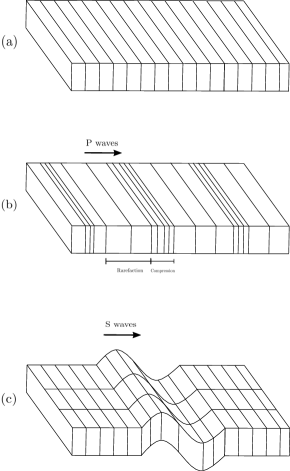
Figure 1: In (a) we have the elastic body in a rest position. In (b) we have the effect of $P$-waves propagation on the material, where small contraction and dilation are produced in the same direction of the wave propagation. In (c) we exemplify the effect of transversal $S$-waves on the material, which are generated from the shear forces and are effective in normal directions with respect to the direction of the wave propagation.

A general existing scenario is when earthquakes generate shear waves, say $S$-waves, that are more effective than compression waves, say $P$-waves, and therefore the most damage on the body displacements is due to the “stronger” vibrations caused by $S$-waves. On the other hand, $P$-waves commonly propagate at a higher speed in relation to $S$-waves, reaching their highest speed, namely, the highest value for $\beta$, near the basis of the body. Thus, from this viewpoint, it is worth mentioning that the approximation $\lambda\to-\mu$ symbolizes the approaching of the velocities with respect to $S$-waves in relation to $P$-waves.

For instance, when one considers the approach of $\lambda$ to $-\mu$ on sedimentary rocks, one has atypical cases concerning bulk modulus or Poisson’s ratio. This is the case when one considers e.g. $\lambda<-\frac{2\mu}{3}$ which is the case where we have negative bulk modulus or when $\lambda\sim-\mu$ which is the case where the Poisson’s ratio is not defined, being $\pm\infty$ in the left or right approximation, respectively. These results seem to contradict the physical notion that we have regarding the study of thermodynamics on this type of materials, but several studies show that the compressibility of the material is closely related to the constant $\lambda$ instead of approximations coming from the bulk modulus or the Poisson’s ratio, see e.g. Goodway [14].

Other examples of such approximations are considered as follows. Indeed, in Moore et al. [27] the authors reveal the possibility of considering negative incremental bulk modulus on open cell foams on porous media. Also, Lakes and Wojciechowski [22] show the possibility of taking negative Poisson’s ratio and bulk modulus for the same type of materials, which proves its structural stability. These are examples that show us the existence of materials (e.g., gas sands [14] and open cell foams [27, 22]) that, under certain circumstances, allow us to consider the limit situation of $\lambda$ to negative values. Thus, it makes sense to consider for example $\lambda\to-\mu$.

Moreover, in Ji et al. [19] the authors show that for quartz materials under a confining pressure of $600$ MPa and a temperature around $650\,^{0}$C, the transmission between High–Low Quartz demonstrates a significant decreasing in the speed of $P$-wave propagation $\left(\alpha=\sqrt{\frac{\lambda+2\mu}{\rho}}\right)$ in relation to the perturbation of the speed of $S$-wave propagation $\left(\beta=\sqrt{\frac{\mu}{\rho}}\right)$. Therefore, to consider the approximation

$$\frac{\alpha}{\beta}\to 1\quad\mbox{ wich means }\quad\lambda\to-\mu$$

in the dynamic of seismic waves, it is equivalent to study the state of transition between High–Low Quartz in materials (say rocks) containing quartz (as for example granite, diorite, and felsic gneiss) and its behavior with respect to the wave speeds of propagation for transverse and compressible waves in the material, under proper conditions of temperature and pressure.

2.2 Assumptions

The following assumptions shall be considered throughout this paper for the functions defined on a bounded domain $\Omega\subset\mathbb{R}^{3}$ with smooth boundary $\partial\Omega$.

1. The damping coefficient $\alpha$ and the Lamé coefficients $\lambda,\mu$ fulfill

   $$\alpha,\mu>0\ \ \mbox{ and }\ \ \lambda\in\mathbb{R}\ \ \mbox{with}\ \ \mu+\lambda\geq 0.$$ (2.2)

2. The external vector force $b$ satisfies

   $$b\in(L^{2}(\Omega))^{3}.$$ (2.3)

3. The nonlinear vector field $f=(f_{1},f_{2},f_{3})$ is assumed to satisfy: there exist a vector field $g=(g_{1},g_{2},g_{3})\in(C^{1}(\mathbb{R}^{3}))^{3}$, and functions $G\in C^{2}(\mathbb{R}^{3})$ and $h_{i}\in C^{2}(\mathbb{R})$, $i=1,2,3$, such that

   $$f_{i}(u_{1},u_{2},u_{3})=g_{i}(u_{1},u_{2},u_{3})+h_{i}(u_{i}),\quad i=1,2,3,$$

   $$f_{i}(0)=g_{i}(0)=h_{i}(0)=0,\quad i=1,2,3,$$

   $$g=(g_{1},g_{2},g_{3})=\nabla G.$$

   In addition, there exist constants $M,m_{f}\geq 0$ such that

   $$f(u)\cdot u-G(u)-\sum_{i=1}^{3}\int_{0}^{u_{i}}h_{i}(s)ds\geq-M|u|^{2}-m_{f},\,\,\forall u\in\mathbb{R}^{3},$$ (2.4)

   $$G(u)+\sum_{i=1}^{3}\int_{0}^{u_{i}}h_{i}(s)ds\geq-M|u|^{2}-m_{f},\,\,\forall u\in\mathbb{R}^{3},$$ (2.5)

   with

   $$0\leq M<\frac{\mu\lambda_{1}}{2},$$ (2.6)

   where $\lambda_{1}>0$ denotes the first eigenvalue of the Laplacian operator $-\Delta$. Moreover, with respect to functions $g_{i}$ and $h_{i}$, $i=1,2,3$, we additionally assume:

   • $g$ fulfills the subcritical growth restriction: there exist $1\leq p<3$ and $M_{g}>0$ such that, for $i=1,2,3$,

     $$|\nabla g_{i}(u)|\leq M_{g}(1+|u_{1}|^{p-1}+|u_{2}|^{p-1}+|u_{3}|^{p-1}),\ \ \forall\,u=(u_{1},u_{2},u_{3})\in\mathbb{R}^{3}.$$ (2.7)

   • For each $i=1,2,3$, $h_{i}$ fulfills the critical growth restriction: there exists a constant $c_{h}>0$ such that

     $$|h^{\prime}_{i}(x)|\leq c_{h}(1+|x|^{2}),\quad\forall\ x\in\mathbb{R},\ i=1,2,3.$$ (2.8)

2.3 Functional setting

We denote the inner product in $L^{2}(\Omega)$ by $\left\langle u,v\right\rangle=\int_{\Omega}uvdx$ for $u,v\in L^{2}(\Omega)$. For the sake of simplicity, we use the same notation to the inner product in $(L^{2}(\Omega))^{3}$, that is, given $u=(u_{1},u_{2},u_{3}),v=(v_{1},v_{2},v_{3})\in(L^{2}(\Omega))^{3}$,

$$\left\langle u,v\right\rangle:=\sum_{i=1}^{3}\left\langle u_{i},v_{i}\right\rangle.$$

Similarly, $\left\langle\nabla\cdot,\nabla\cdot\right\rangle$ stands for the inner product in $H_{0}^{1}(\Omega)$ as well as the inner product in $(H_{0}^{1}(\Omega))^{3}$. Thus, given $u=(u_{1},u_{2},u_{3}),v=(v_{1},v_{2},v_{3})\in(L^{2}(\Omega))^{3}$,

$$\left\langle\nabla u,\nabla v\right\rangle:=\sum_{i=1}^{3}\left\langle\nabla u_{i},\nabla v_{i}\right\rangle.$$

In addition, for $p>0$, we denote the norms in the spaces $L^{p}(\Omega)$ and $(L^{p}(\Omega))^{3}$ by $|\cdot|_{p}$ and $\|\cdot\|_{p}$, respectively, that is,

$$|u|_{p}:=\left(\int_{\Omega}|u|^{p}dx\right)^{\frac{1}{p}},\;\;u\in L^{p}(\Omega),$$

$$\|u\|_{p}^{p}:=\sum_{i=1}^{3}|u_{i}|_{p}^{p},\;\;u=(u_{1},u_{2},u_{3})\in(L^{p}(\Omega))^{3}.$$

In particular, for $p=2$, one reads

$$\|u\|_{2}^{2}=\left\langle u,u\right\rangle\ \mbox{ for }\ u\in(L^{2}(\Omega))^{3}\ \ \mbox{and}\ \ |u|_{2}^{2}=\left\langle u,u\right\rangle\ \mbox{ for }\ u\in L^{2}(\Omega).$$

The elasticity operator $\mathcal{E}$, with domain $D(\mathcal{E}):=(H^{2}(\Omega)\cap H_{0}^{1}(\Omega))^{3}$, is given by

$${\mathcal{E}}u=-\mu\Delta u-(\lambda+\mu)\nabla(\nabla\cdot u).$$ (2.9)

We consider the Hilbert space $\left((H_{0}^{1}(\Omega))^{3},\left\langle\cdot,\cdot\right\rangle_{e}\right)$, where the inner product $\left\langle\cdot,\cdot\right\rangle_{e}$ is given by

$$\left\langle v,w\right\rangle_{e}=\mu\left\langle\nabla v,\nabla w\right\rangle+(\lambda+\mu)\left\langle\text{div}u,\text{div}w\right\rangle.$$

Remark 2.1.

Under the above notations, it is easy to verify that the norms $\|\cdot\|_{e}^{2}:=\sqrt{\left\langle\cdot,\cdot\right\rangle_{e}}$ and $\|\nabla\cdot\|_{2}^{2}:=\sqrt{\left\langle\nabla\cdot,\nabla\cdot\right\rangle}$ are equivalent in $(H_{0}^{1}(\Omega))^{3}$. More precisely, one has

$$\mu\|\nabla u\|_{2}^{2}\leq\|u\|_{e}^{2}\leq a_{0}\|\nabla u\|_{2}^{2},\ \ \forall\,u=(u_{1},u_{2},u_{3})\in(H_{0}^{1}(\Omega))^{3},$$

where $a_{0}=\max\{\mu,3(\lambda+\mu)\}$.

Additionally, if $u\in D(\mathcal{E})$ and $v\in(H_{0}^{1}(\Omega))^{3}$, then it is easy to verify that

$$\left\langle\mathcal{E}u,v\right\rangle=\left\langle u,v\right\rangle_{e}.$$ (2.10)

From (2.10), Remark 2.1 and the compact embedding of $H_{0}^{1}(\Omega)\hookrightarrow L^{2}(\Omega)$, one sees that $\mathcal{E}$ is a positive self-adjoint operator. We denote the fractional power associated to $\mathcal{E}$ by $\mathcal{E}^{r}$ with domain $X^{r}:=D({\mathcal{E}}^{r})$, which is endowed with the natural inner product $\left\langle\cdot,\cdot\right\rangle_{r}:=\left\langle{\mathcal{E}}^{r}\cdot,{\mathcal{E}}^{r}\cdot\right\rangle$. In particular,

$$X^{0} =((L_{2}(\Omega))^{3};\left\langle\cdot,\cdot\right\rangle),$$

$$X^{1/2} =\left((H_{0}^{1}(\Omega))^{3};\left\langle{\mathcal{E}}^{1/2}\cdot,{\mathcal{E}}^{1/2}\cdot\right\rangle\right),$$

$$X^{1} =(D({\mathcal{E}});\left\langle\mathcal{E}\cdot,\mathcal{E}\cdot\right\rangle).$$

Remark 2.2.

From Riesz’s Theorem along with density arguments and continuity, we have

$$\left\langle u,v\right\rangle_{1/2}=\left\langle u,v\right\rangle_{e},\quad\forall\ u,v\in(H_{0}^{1}(\Omega))^{3}.$$

Finally, we define the (Hilbert) weak phase space $\mathcal{H}:=X^{1/2}\times X^{0}$ with the usual inner product and induced norm $\|\cdot\|_{\mathcal{H}}$; and the (Hilbert) strong phase space $\mathcal{H}^{1}:=X^{1}\times X^{1/2}.$

2.4 Well-posedness and energy estimates

Under the above assumptions and notations, we are able to state the Hadamard well-posedness of $(\ref{problem})$. We start by denoting

$$U=\left[\begin{array}[]{c}u\\ \partial_{t}u\end{array}\right],\ \ \mathbb{E}=\left[\begin{array}[]{cc}0&-I\\ \mathcal{E}&\alpha\end{array}\right],\ \ \mathbb{F}=\left[\begin{array}[]{cc}0&0\\ f(\cdot)&0\end{array}\right],\ \ \mathbb{B}=\left[\begin{array}[]{c}0\\ b(x)\end{array}\right].$$ (2.11)

Then, problem (1.9) is equivalent to the Cauchy problem

$$\partial_{t}U+\mathbb{E}U+\mathbb{F}U=\mathbb{B},\ \ U(0)=\left[\begin{array}[]{c}u_{0}\\ u_{1}\end{array}\right],$$ (2.12)

where $\mathbb{E}:D(\mathbb{E})\subset\mathcal{H}\to\mathcal{H}$ with domain

$$D(\mathbb{E})=\{(u,v)\in\mathcal{H}\ |\ \mathcal{E}u+\alpha v\in X^{0},\,v\in X^{1/2}\}=\mathcal{H}^{1}.$$

Theorem 2.1 (Well-posedness).

Let us assume that $(\ref{2})$-$(\ref{aa})$ hold. Then,

• For $(u_{0},u_{1})\in\mathcal{H}$, system $(\ref{abs-system})$ possesses a unique mild solution

  $$U\in C(\mathbb{R}^{+};\mathcal{H}).$$

• For $(u_{0},u_{1})\in\mathcal{H}^{1}$, system $(\ref{abs-system})$ possesses a unique regular solution

  $$U\in C(\mathbb{R}^{+};\mathcal{H}^{1}).$$

• For any $T>0$ and any bounded set $B\subset\mathcal{H}$, there exists a constant $C_{BT}>0$ such that for any two solutions $z^{i}=(u^{i},\partial_{t}u^{i})$ of (2.12) with initial data $z_{0}^{i}\in B$, $i=1,2$, we have

  $$\|z^{1}(t)-z^{2}(t)\|_{\mathcal{H}}^{2}\leq C_{BT}\|z_{0}^{1}-z_{0}^{2}\|_{\mathcal{H}}^{2}.$$

Proof.

It is easy to check that operator $\mathbb{E}$ set in (2.11) is a maximal monotone operator and also, under assumption (A3), $\mathbb{F}$ is a locally Lipschitz on $\mathcal{H}$. Therefore, applying the classical theory of linear semigroups, see e.g. [3, 15, 28], items $(i)$-$(ii)$ are concluded. The continuous dependence $(iii)$ is also obtained by using standard computations in the difference of solutions. ∎

In what follows we give some useful inequalities involving the energy functional. The total energy functional associated with problem (1.9) is given by

$$E(t)=\frac{1}{2}\|(u,\partial_{t}u)\|_{\mathcal{H}}^{2}+\int_{\Omega}G(u)dx+\sum_{i=1}^{3}\int_{\Omega}\int_{0}^{u_{i}}h_{i}(s)dsdx-\left\langle b(x),u\right\rangle.$$ (2.13)

Proposition 1.

Under the hypotheses $(\ref{2})$-$(\ref{aa})$, we have:

• the energy $E(t)$ is non-increasing with $E(t)\leq E(0)$ for all $t\geq 0;$

• there exist positive constants $K_{1},K_{2}$ and $K_{3}$ such that

  $$K_{2}\|(u,\partial_{t}u)\|_{\mathcal{H}}^{2}-K_{3}\leq E(t)\leq K_{1}\|(u,\partial_{t}u)\|_{\mathcal{H}}^{4}+K_{3},\ \ \forall\,t\geq 0.$$ (2.14)

Proof.

$(i)$ Taking the multiplier $u_{t}$ in problem (1.9), then a straightforward computation leads us to

$$E^{\prime}(t) =-\alpha\|\partial_{t}u\|_{2}^{2}\leq 0,\quad\forall\ t>0,$$ (2.15)

from where it readily follows the stated in item $(i)$.

$(ii)$ From conditions $(\ref{2})$-$(\ref{aa})$ and Young’s inequality with $\epsilon>0$, the expression

$$I=\int_{\Omega}G(u)dx+\sum_{i=1}^{3}\int_{\Omega}\int_{0}^{u_{i}}h_{i}(s)dsdx-\left\langle b(x),u\right\rangle$$

can be estimated from below and above as follows

$$I \geq\,-\ m_{f}|\Omega|-\frac{\epsilon}{4}\|b\|_{2}^{2}-\left(\frac{M}{\lambda_{1}\mu}+\frac{1}{\lambda_{1}\mu\epsilon}\right)\|(u,\partial_{t}u)\|_{\mathcal{H}}^{2},$$

$$I \leq C_{f}|\Omega|+\frac{1}{2}\|b\|_{2}^{2}+\frac{C_{g}}{\mu^{\frac{p+1}{2}}}\|(u,\partial_{t}u)\|_{\mathcal{H}}^{p+1}$$

$$\ \ \ \ +\frac{C_{h}}{\mu^{2}}\|(u,\partial_{t}u)\|_{\mathcal{H}}^{4}+\frac{1}{2\sqrt{\lambda_{1}}\mu}\|(u,\partial_{t}u)\|_{\mathcal{H}}^{2},$$

where the positive generic constants depend on their index and some embedding with $H_{0}^{1}(\Omega)$, for example $C_{h}$ depends on the constant $c_{h}$ in (2.8) and the compact embedding $H_{0}^{1}(\Omega){\hookrightarrow}L^{4}(\Omega)$. From this and the definition of $E(t)$ in (2.13), we infer

$$E(t) \leq C_{f}|\Omega|+\frac{1}{2}\|b\|_{2}^{2}+\frac{1}{2\sqrt{\lambda_{1}}\mu}+\frac{C_{g}}{\mu^{\frac{p+1}{2}}}$$

$$\ \ \ +\left(\frac{1}{2}+\frac{C_{g}}{\mu^{\frac{p+1}{2}}}+\frac{C_{h}}{\mu^{2}}\right)\|(u,\partial_{t}u)\|_{\mathcal{H}}^{4},$$

$$E(t) \geq-m_{f}|\Omega|-\frac{\epsilon}{4}\|b\|_{2}^{2}+\left(\frac{1}{2}-\frac{M}{\lambda_{1}\mu}-\frac{1}{\lambda_{1}\mu\epsilon}\right)\|(u,\partial_{t}u)\|_{\mathcal{H}}^{2}.$$

Therefore, from a proper choice of $\epsilon>0$ and using condition (2.6), one can conclude the existence of positive constants $K_{1},K_{2}$ and $K_{3}$ satisfying (2.14). ∎

Remark 2.3.

We emphasizes that above constants $K_{1},K_{2}$ and $K_{3}$ in $(\ref{18})$ do not depend on the parameter $\lambda$.

3 Long-time dynamics

From Theorem 2.1, one can define a dynamical system $(\mathcal{H},S(t))$ associated with problem $(\ref{problem})$, where the evolution operator $S(t)$ corresponds to a non-linear $C_{0}$-semigroup (locally Lipschitz) on $\mathcal{H}$.

Our main goal in this section is to prove that $(\mathcal{H},S(t))$ possesses a finite dimensional global attractor $\mathcal{A}$ as well as to reach its qualitative properties such as characterization and regularity. To this end, we first recall some concepts in the theory of dynamical systems, by following e.g. the references [10, 11].

3.1 Some elements of dynamical systems

For the sake of completeness, we recall some basic facts on dynamical systems.

• A global attractor for a dynamical system $(\mathcal{H},S(t))$ is a compact set $\mathcal{A}\subset\mathcal{H}$ which is fully invariant and uniformly attracting, it means, for any bounded subset $B\subset\mathcal{H}$

  $$S(t)\mathcal{A}=\mathcal{A}\text{ and }\lim_{t\to\infty}d_{\mathcal{H}}(S(t)B,\mathcal{A})=0.$$

• The fractal dimension of a compact set $B\subset\mathcal{H}$ is defined as

  $$\dim_{f}B=\limsup_{\epsilon\to 0}\frac{lnN_{\epsilon}(B)}{ln(1/\epsilon)},$$

  where $N_{\epsilon}(B)$ is the minimal number of closed balls of radius $2\epsilon$ necessary to cover $B$.

• The set of stationary points $\mathcal{N}$ of a dynamical system $(\mathcal{H},S(t))$ is defined as

  $$\mathcal{N}=\left\{V\in\mathcal{H}\ |\ S(t)V=V,\ \ \forall\,t>0\right\}.$$

• A dynamical system $(\mathcal{H},S(t))$ is called gradient if there exists a strict Lyapunov functional $\Psi$, that is, for any $z\in\mathcal{H}$, $\Psi(S(t)z)$ is decreasing with respect $t\geq 0$ and $\Psi$ is constant on the set of stationary points $\mathcal{N}$.

• Given a set $B\subset\mathcal{H}$, its unstable manifold $W^{u}(B)$ is the set of points $z\in\mathcal{H}$ that belongs to some complete trajectory $\{y(t)\}_{t\in\mathbb{R}}$ and satisfies

  $$y(0)=z\text{ and }\limsup_{t\to-\infty}\text{dist}(y(t),B)=0.$$

• Quasi-stability. Let $X,Y$ be reflexive Banach spaces with compact embedding $X\overset{c}{\hookrightarrow}Y$ and $\mathcal{H}=X\times Y$. Let us suppose $(\mathcal{H},S(t))$ is given by

  $$S(t)z=(u(t),\partial_{t}u(t)),\,\,z=(u_{0},u_{1})\in\mathcal{H},$$

  where

  $$u\in C(\mathbb{R}^{+};X)\cap C^{1}(\mathbb{R}^{+};Y),$$

  Then, $(\mathcal{H},S(t))$ is called quasi-stable on a set $B\subset\mathcal{H}$ if there exists a compact semi-norm $\eta_{X}$ on $X$ and non-negative scalar functions $a_{1}(t)$ and $a_{3}(t)$ locally bounded in $\mathbb{R}^{+}$ and $a_{2}(t)\in L^{1}(\mathbb{R}^{+})$ with $\lim_{t\to\infty}a_{2}(t)=0$ such that

  $$\|S(t)z^{1}-S(t)z^{2}\|_{\mathcal{H}}^{2}\leq a_{1}(t)\|z^{1}-z^{2}\|_{\mathcal{H}}^{2},$$

  and

  $$\|S(t)z^{1}-S(t)z^{2}\|_{\mathcal{H}}^{2}\leq a_{2}(t)\|z^{1}-z^{2}\|_{\mathcal{H}}^{2}+a_{3}(t)\sup_{0\leq s\leq t}\left[\eta_{X}(u^{1}(s)-u^{2}(s))\right]^{2},$$

  for any $z^{1},z^{2}\in B$.

Proposition 2 ([11, Corollary 7.5.7]).

Let $(\mathcal{H},S(t))$ be a gradient asymptotically smooth dynamical system. Additionally, if its Lyapunov function $\Psi(x)$ is bounded from above on any bounded subset of $\mathcal{H}$, the set $\Psi_{R}=\left\{x\in\mathcal{H}:\Psi(x)\leq R\right\}$ is bounded for every $R$ and the set $\mathcal{N}$ of stationary points of $(\mathcal{H},S(t))$ is bounded, then $(\mathcal{H},S(t))$ possesses a compact global attractor characterized by $\mathcal{A}=W^{u}(\mathcal{N})$.

Proposition 3 ([11, Proposition 7.9.4]).

Let us assume that the dynamical system $(\mathcal{H},S(t))$ is quasi-stable on every bounded forward invariant set $B\subset\mathcal{H}.$ Then, $(\mathcal{H},S(t))$ is asymptotically smooth.

Proposition 4 ([11, Theorem 7.9.6]).

Let $(\mathcal{H},S(t))$ a quasi-stable dynamical system. If $(\mathcal{H},S(t))$ possesses a compact global attractor $\mathcal{A}$ and is quasi-stable on $\mathcal{A}$, hen the attractor $\mathcal{A}$ has a finite fractal dimension $\dim_{f}\mathcal{A}<\infty.$

3.2 Main result and proofs

We are now in condition to state and prove the main result concerning global attractors associated with problem $(\ref{problem})$. It reads as follows.

Theorem 3.1.

Under the assumptions $(\ref{2})$-$(\ref{aa})$, we have:

• The dynamical system $(\mathcal{H},S(t))$ corresponding to problem (1.9) has a unique global attractor $\mathcal{A}$ with finite fractal dimension $\dim_{f}\mathcal{A}<\infty$, and is characterized by the unstable manifold $\mathcal{A}=W^{u}(\mathcal{N})$ emanating from the set of stationary points $\mathcal{N}$ of $(\mathcal{H},S(t))$.

• Moreover, if $h_{i}=0$, $i=1,2,3$, then $\mathcal{A}$ is bounded in the strong phase space $\mathcal{H}^{1}$. In particular, any full trajectory $\{(u(t),\partial_{t}u(t)),t\in\mathbb{R}\}$ that belongs to $\mathcal{A}$ has the following regularity properties

  $$\partial_{t}u\in L^{\infty}(\mathbb{R};(H_{0}^{1}(\Omega))^{3})\cap C(\mathbb{R};(L^{2}(\Omega))^{3}),\,\,\,\partial^{2}_{t}u\in L^{\infty}(\mathbb{R};(L^{2}(\Omega))^{3}),$$ (3.1)

  and there exists $R>0$ such that

  $$\|(\partial_{t}u(t),\partial^{2}_{t}u(t))\|_{\mathcal{H}}^{2}\leq R^{2},$$ (3.2)

  where $R$ does not depend on $\lambda$.

The proof of Theorem 3.1 will be concluded at the end of this section as a consequence of some technical results provided in the sequel.

3.2.1 Gradient property

Lemma 3.2.

Under the assumptions of Theorem $\ref{3.16},$ let us define the functional

$$\begin{array}[]{rcl}\Psi:\,\mathcal{H}&\rightarrow&\mathbb{R}\\ z&\mapsto&\Psi(z):=\Psi(u,v)\end{array}$$

given by

$$\Psi(u,v)=\frac{1}{2}\|(u,v)\|_{\mathcal{H}}^{2}+\int_{\Omega}G(u)dx+\sum_{i=1}^{3}\int_{\Omega}\int_{0}^{u_{i}}h_{i}(s)dsdx-\left\langle b(x),u\right\rangle.$$ (3.3)

Then:

1. $\Psi$ is a strict Lyapunov functional;

2. $\Psi(z)\rightarrow\infty$ if and only if $\|z\|_{\mathcal{H}}\rightarrow\infty$;

3. $\mathcal{N}$ is bounded on $\mathcal{H}$

As a consequence, the dynamical system $(\mathcal{H},S(t))$ associated with problem (1.9) is a gradient system.

Proof.

Let fix $z_{0}\in\mathcal{H}$ and recall that $\mathcal{N}$ is the set of stationary points of $(\mathcal{H},S(t))$. Also, from (2.13) one sees that $\Psi(u(t),\partial_{t}u(t))=E(u(t),\partial_{t}u(t)):=E(t)$. Then, we infer:

• From (2.15), it is clear that $\Psi(S(t)z_{0})$ is decreasing with respect to time and from (2.14), $\Psi(z)=\Psi(S(0)z)\rightarrow\infty$ if and only if $||z||_{\mathcal{H}}\rightarrow\infty$.

• Let us consider the stationary problem:

  $$\left\{\begin{array}[]{lcr}\mathcal{E}u+f(u)=b(x)&\text{in}&\Omega,\\ u=0&\text{on}&\partial\Omega.\end{array}\right.$$ (3.6)

  Thus, a simple computation shows that $\mathcal{N}$ is given by

  $$\mathcal{N}=\left\{(u,0)\in\mathcal{H}\ |\ u\text{ is the solution of }(\ref{bb})\right\}.$$

  In addition, from (2.15) it is easy to prove that $\Psi$ is constant on $\mathcal{N}$. Finally, multiplying (3.6) by $u$, integrating on $\Omega$ and using (2.4) and (2.5), we obtain that for any $\epsilon>0$

  $$\left(1-\frac{2M}{\lambda_{1}\mu}-\frac{1}{4\lambda_{1}\mu\epsilon}\right)\|u\|_{e}^{2} \leq 2m_{f}|\Omega|+\epsilon\|b\|_{2}^{2},$$ (3.7)

  from where (along with (2.6)) we conclude that $\mathcal{N}$ is bounded on $\mathcal{H}$, for $\epsilon>0$ properly chosen.

Therefore, the items 1 - 3 are proved. ∎

3.2.2 Quasi-stability property

Proposition 5 (Stabilizability Estimate).

Under the assumptions of Theorem $\ref{3.16},$ let us consider a bounded subset $B\subset\mathcal{H}$ and two weak solutions $\tilde{z}=(v,\partial_{t}v)$ and $z=(u,\partial_{t}u)$ of problem $(\ref{problem})$ with initial data $\tilde{z}(0)=(v_{0},v_{1})$, $z(0)=(u_{0},u_{1})\in B$. Then,

$$\|\tilde{z}(t)-z(t)\|_{\mathcal{H}}^{2}\leq a_{2}(t)\|\tilde{z}(0)-z(0)\|_{\mathcal{H}}^{2}+c(t)\sup_{0\leq s\leq t}\|v-u\|_{p_{0}}^{2},$$ (3.8)

where $p_{0}=\max\{4,\frac{6}{4-p}\}<6$, $b\in L^{1}(\mathbb{R}^{+})$ with $\displaystyle\lim_{t\to\infty}a_{2}(t)=0$ and $c(t)$ is a locally bounded function.

Proof.

The estimate (3.8) is one of the main cores of the present article. Its proof is quite technical and long, and for this reason we are going to proceed in several steps as follows.

Step 1. Setting the difference problem and functionals. Let us denote $w=u-v$. Then, a simple computation shows that $w$ is a solution (in the weak and strong sense) of the following problem

$$\left\{\begin{array}[]{lcr}\partial^{2}_{t}w+\mathcal{E}w+\alpha\partial_{t}w+f(u)-f(v)=0&\text{on}&\Omega\times\mathbb{R}^{+},\vskip 3.0pt plus 1.0pt minus 1.0pt\\ w=0&\text{in}&\partial\Omega\times\mathbb{R}^{+},\vskip 3.0pt plus 1.0pt minus 1.0pt\\ w(x,0)=u_{0}(x)-v_{0}(x),\ x\in\Omega,&&\vskip 3.0pt plus 1.0pt minus 1.0pt\\ \partial_{t}w(x,0)=u_{1}(x)-v_{1}(x),\ x\in\Omega.&&\end{array}\right.$$ (3.13)

The energy associated with system (3.13) is given by

$$\Xi(t):=\frac{1}{2}\|(w,\partial_{t}w)\|_{\mathcal{H}}^{2}=\frac{1}{2}\|\tilde{z}(t)-z(t)\|_{\mathcal{H}}^{2},\ \ t\geq 0.$$ (3.14)

We also set the functional

$$\chi(t) =\left\langle w,\partial_{t}w\right\rangle,$$

and the perturbed energy functional

$$\Upsilon(t)=\epsilon_{1}\Xi(t)+\epsilon_{2}\chi(t),$$

where the constants $\epsilon_{1},\epsilon_{2}>0$ will be chosen later.

Step 2. Equivalence. There exist constants $C_{1},C_{2}>0$ such that

$$C_{2}\Xi(t)\leq\Upsilon(t)\leq C_{1}\Xi(t).$$ (3.15)

Indeed, the inequalities in (3.15) follow by taking $K^{\prime}=\max\{\frac{C^{2}}{\mu},1\}$, $\epsilon_{1}>\epsilon_{2}K^{\prime}$, $C_{2}=\epsilon_{1}-\epsilon_{2}K^{\prime}$ and $C_{1}=\epsilon_{1}+\epsilon_{2}K^{\prime}$.

Step 3. Estimate for $\Xi^{\prime}$. Given $\xi>0$, there exists a constant $C(\xi,B)>0$, which depends on $\xi$ and $B$, such that

$$\Xi^{\prime}(t)\leq-{\alpha}\|\partial_{t}w\|_{2}^{2}+C(\xi,B)\|w\|_{\frac{6}{4-p}}^{2}+\xi\|\partial_{t}w\|_{2}^{2}+I,$$ (3.16)

where we set

$$I:=\displaystyle\sum_{i=1}^{3}\left\langle h_{i}(v_{i})-h_{i}(u_{i}),\partial_{t}w_{i}\right\rangle.$$ (3.17)

In fact, we first observe that deriving $\Xi(t)$ and using (3.13), we get

$$\Xi^{\prime}(t)= -\alpha\|\partial_{t}w\|_{2}^{2}-\left\langle g(u)-g(v),\partial_{t}w\right\rangle+I.$$

Since

$$|\left\langle g(u)-g(v),\partial_{t}w\right\rangle|\leq\sum_{i=1}^{3}\int_{\Omega}M_{g}\left\{1+\sum_{i=1}^{3}|v_{i}|^{p-1}+\sum_{i=1}^{3}|u_{i}|^{p-1}\right\}|w||\partial_{t}w_{i}|dx,$$

then applying Hölder’s inequality, we obtain

$$|\left\langle g(u)-g(v),\partial_{t}w\right\rangle|\leq\sum_{i=1}^{3}\tilde{C}_{f}\|w\|_{\frac{6}{4-p}}\|\partial_{t}w_{i}\|_{2},$$ (3.18)

where

$$\tilde{C}_{f}=M_{f}\left\{|\Omega|^{\frac{p-1}{6}}+\sum_{i=1}^{3}\|v_{i}\|_{6}^{p-1}+\sum_{i=1}^{3}\|u_{i}\|_{6}^{p-1}\right\}\leq C(B)<\infty,$$

is a constant depending on $B$. Therefore, the estimate (3.16) follows from Young’s inequality with $\xi>0$.

Step 4. Estimate for $\chi^{\prime}$. There exists a constant $C(B)>0$ depending on $B$ such that

$$\chi^{\prime}(t)\leq-\Xi(t)-\frac{1}{2}\|w\|_{e}^{2}+\frac{\alpha}{2}\|w\|_{2}^{2}+C(B)\|w\|_{4}^{2}+\frac{3+\alpha}{2}\|\partial_{t}w\|_{2}^{2}.$$ (3.19)

Indeed, multiplying (3.13)₁ by $w$ and integrating on $\Omega$, we obtain

$$\chi^{\prime}(t) =-\Xi(t)-\frac{1}{2}\|w\|_{e}^{2}+\frac{\alpha}{2}\|w\|_{2}^{2}+\frac{\alpha+3}{2}\|\partial_{t}w\|_{2}^{2}$$

$$\hskip 85.35826pt-\left\langle g(u)-g(v),w\right\rangle+\sum_{i=1}^{3}\left\langle h_{i}(u_{i})-h_{i}(v_{i}),w_{i}\right\rangle.$$

Now, noting that

$$\left\langle g(v)-g(u),w\right\rangle\leq 3\left\{|\Omega|^{p-1}+\sum_{i=1}^{3}\|u_{i}\|_{p+1}^{p-1}+\sum_{i=1}^{3}\|v_{i}\|_{p+1}^{p-1}\right\}\|w\|_{p+1}^{2}\leq\tilde{C}_{B}\|w\|_{p+1}^{2},$$

and

$$\sum_{i=1}^{3}\left\langle h_{i}(u_{i})-h_{i}(v_{i}),w_{i}\right\rangle\leq\sum_{i=1}^{3}(|\Omega|^{2}+\|v_{i}\|_{4}^{2}+\|u_{i}\|_{4}^{2})|w_{i}|_{4}^{2}\leq C_{B}\|w\|_{4}^{2},$$

where the constants $\tilde{C}_{B},C_{B}>0$ depend only on $B$, then the estimate (3.19) follows.

Step 5. Estimate for $\Upsilon$. There exists a constant $C_{3}>0$ depending on $B$ such that

$$\Upsilon(t)\leq e^{-\frac{\epsilon_{2}t}{C_{1}}}\Upsilon(0)+C_{3}\int_{0}^{t}e^{-\frac{\epsilon_{2}}{C_{1}}(t-s)}\|w(s)\|_{p_{0}}^{2}ds+\epsilon_{1}e^{-\frac{\epsilon_{2}t}{C_{1}}}J,$$ (3.20)

where $C_{1}>0$ comes from (3.15) and we set

$$J:=\int_{0}^{t}e^{\frac{\epsilon_{2}s}{C_{1}}}Ids=\sum_{i=1}^{3}\int_{0}^{t}e^{\frac{\epsilon_{2}s}{C_{1}}}\left\langle h_{i}(v_{i}(x,s))-h_{i}(u_{i}(x,s)),\partial_{t}w_{i}(x,s)\right\rangle ds.$$ (3.21)

First, we note that from (3.16) and (3.19), one has

$$\Upsilon^{\prime}(t)\leq -\epsilon_{2}\Xi(t)+\frac{\alpha\epsilon_{2}}{2}\|w\|_{2}^{2}+\epsilon_{2}C(B)\|w\|_{4}^{2}+\epsilon_{1}C(\xi,B)\|w\|_{\frac{6}{4-p}}^{2}$$

$$\ +\epsilon_{1}I+\left(\frac{3\epsilon_{2}+\alpha\epsilon_{2}}{2}+\epsilon_{1}\xi-\alpha\epsilon_{1}\right)\|\partial_{t}w\|_{2}^{2}.$$

We now choose $\epsilon_{1},\epsilon_{2},\xi>0$ small enough such that

$$\epsilon_{2}K^{\prime}<\epsilon_{1}\quad\mbox{ and }\quad\frac{3\epsilon_{2}+\alpha\epsilon_{2}}{2}+\epsilon_{1}\xi<\alpha\epsilon_{1}.$$

It is worth mentioning that $\epsilon_{1},\epsilon_{2},\xi>0$ do not depend on $\lambda$. Thus, from this choice, setting $p_{0}=\max\{\frac{6}{4-p},4\}$ and using (3.15), there exists a constant $C_{3}=C(B)>0$ such that

$$\Upsilon^{\prime}(t) \leq-\frac{\epsilon_{2}}{C_{1}}\Upsilon(t)+C_{3}\|w\|_{p_{0}}^{2}+\epsilon_{1}I,$$

from where it follows the estimate (3.20) with $J$ given in (3.21).

Remark 3.1.

Since the choices for $\epsilon_{1},\epsilon_{2}$ do not depend on $\lambda$, then $C_{3}>0$ is a constant that does not depend on $\lambda$ as well.

Step 6. Estimate for $J$. There exist constants $\gamma_{0}>0$ and $C_{4}>0$ depending on $B$ such that

$$J\leq C_{4}e^{\gamma_{0}t}\sup_{0<s<t}\|w\|_{4}^{2}+C_{4}\int_{0}^{t}(\|\partial_{t}u(s)\|_{2}+\|\partial_{t}v(s)\|_{2})e^{\gamma_{0}s}\Upsilon(s)ds.$$ (3.22)

Firstly, in view of assumption (2.8) and following verbatim the same arguments as in [8, Lemma 4.9], for any constant $\gamma>0$ and each $i=1,2,3,$ there exists a constant $K_{i}^{\prime}>0$ such that

$$\int_{0}^{t}e^{\gamma s} \left\langle h_{i}(v_{i}(s))-h_{i}(u_{i}(s)),\partial_{t}w_{i}(s)\right\rangle ds$$

$$\leq K_{i}^{\prime}e^{\gamma t}\sup_{0<s<t}\|w_{i}\|_{4}^{2}+K_{i}^{\prime}\int_{0}^{t}\left(|u_{i}^{\prime}(s)|_{2}+|v_{i}^{\prime}(s)|_{2}\right)e^{\gamma s}|\nabla w_{i}(s)|_{2}^{2}ds.$$ (3.23)

Therefore, from (3.21) and (3.23) it prompt follows

$$J\leq\sum_{i=1}^{3}K^{\prime}_{i}\sup_{0<s<t}\|w\|_{4}^{2}+\max\{K^{\prime}_{i}\}\int_{0}^{t}e^{\gamma_{0}s}(\|\partial_{t}u\|_{2}+\|\partial_{t}v\|_{2})\|\nabla w(s)\|_{2}^{2}ds,$$

for $\gamma_{0}=\frac{\epsilon_{2}}{C_{1}}>0.$ Additionally, taking $C_{4}=\max\{K^{\prime}_{1}+K^{\prime}_{2}+K^{\prime}_{3},\frac{2\max\{K^{\prime}_{i}\}}{\mu C_{2}}\}>0$ and noting that

$$\|\nabla w(s)\|_{2}^{2}\leq\frac{1}{\mu}\|w\|_{e}^{2}\leq\frac{2}{\mu}\Xi(s)\leq\frac{2}{\mu C_{2}}\Upsilon(s),$$

then estimate (3.22) follows as desired.

Remark 3.2.

We emphasize that constants $\gamma_{0}$ and $C_{4}$ do not depend on $\lambda$.

Step 7. Conclusion of the proof. We are finally in position to complete the proof of (3.8). Indeed, from (3.20) and (3.22), there exists a constant $C_{5}>0$ depending on $B,$ but independently of $\lambda$, such that

$$e^{\gamma_{0}t}\Upsilon(t)\leq \,C_{5}\Upsilon(0)+C_{5}e^{\gamma_{0}t}\sup_{0<s<t}\|w\|_{p_{0}}^{2}$$

$$\ +C_{5}\int_{0}^{t}(\|\partial_{t}u(s)\|_{2}+\|\partial_{t}v(s)\|_{2})e^{\gamma_{0}s}\Upsilon(s)ds,$$

and applying Gronwall’s inequality, one gets

$$\Upsilon(t)\leq C_{5}\left\{e^{-\gamma_{0}t}\Upsilon(0)+\sup_{0<s<t}\|w\|_{p_{0}}^{2}\right\}e^{\left(C_{5}e^{-\gamma_{0}t}\int_{0}^{t}(\|\partial_{t}u(s)\|_{2}+\|\partial_{t}v(s)\|_{2})e^{\gamma_{0}s}ds\right)}.$$ (3.24)

Now, from (2.14) and (2.15), and also in view of Remark 2.3, we have

$$\int_{0}^{t}\|\partial_{t}u(s)\|_{2}^{2}ds=-\frac{1}{\alpha}\int_{0}^{t}E^{\prime}(s)ds\leq\frac{2|E(0)|}{\alpha}\leq Q,$$

where $Q>0$ is a constant depending on $B$ and $f$, but independent of $\lambda.$ The same computation holds true for $\int_{0}^{t}\|\partial_{t}v(s)\|_{2}^{2}ds$. Thus, using Hölder and Young’s inequalities, we obtain

$$e^{-\gamma_{0}t}\int_{0}^{t}(\|\partial_{t}u(s)\|_{2}+\|\partial_{t}v(s)\|_{2})e^{\gamma_{0}s}ds\leq 2\sqrt{Q}\sqrt{t}\leq\epsilon t+\frac{2Q}{\epsilon},$$

for any $t>0$ and $\epsilon>0$. Replacing the latter estimate in (3.24), we arrive at

$$\Upsilon(t) \leq C_{5}e^{(\epsilon C_{5}t+\frac{2C_{5}Q}{\epsilon})}\left\{e^{-\gamma_{0}t}\Upsilon(0)+\sup_{0<s<t}\|w\|_{p_{0}}^{2}\right\}.$$

Taking $\epsilon=\frac{\gamma_{0}}{2C_{4}}$ and using (3.15), we have

$$\Xi(t)\leq\frac{C_{1}C_{4}e^{\frac{Q}{\gamma_{0}}}}{C_{2}}e^{\frac{-\gamma_{0}}{2}t}\Xi(0)+\frac{C_{4}e^{\frac{Q}{\gamma_{0}}}}{C_{2}}e^{\frac{\gamma_{0}}{2}t}\sup_{0<s<t}\|w\|_{p_{0}}^{2}.$$ (3.25)

Finally, regarding the definition of $\Xi(t)$, $t\geq 0$, in (3.14) and setting

$$a_{2}(t):=\frac{C_{1}C_{4}e^{\frac{Q}{\gamma_{0}}}}{C_{2}}e^{\frac{-\gamma_{0}}{2}t}\ \ \mbox{ and }\ \ a_{3}(t):=\frac{2C_{4}e^{\frac{Q}{\gamma_{0}}}}{C_{2}}e^{\frac{\gamma_{0}}{2}t},$$ (3.26)

then (3.25) leads to (3.8) as desired.

The proof of Proposition 5 is therefore concluded. ∎

Corollary 1 (Quasi-stability).

Under the assumptions of Theorem $\ref{3.16},$ the dynamical system $(\mathcal{H},S(t))$ associated with problem (1.9) is quasi-stable on any bounded set $B\subset\mathcal{H}$.

Proof.

It is a direct consequence of Theorem 2.1 - $(iii)$ and Proposition 5 by noting the semi-norm given by $n_{H^{1}_{0}}(v-u)=\|v-u\|_{p_{0}}$ is compact. ∎

3.2.3 Conclusion of the proof of Theorem 3.1

• From Proposition 3 and Corollary 1, the dynamical system $(\mathcal{H},S(t))$ related to problem (1.9) is asymptotically smooth. Therefore, using Lemma 3.2 and Propositions 2 and 4, the conclusion of Theorem 3.1 - $(i)$ is complete.

• In case $h_{i}=0$, $i=1,2,3$, then going back to (3.17), one sees that $I=0$ and, consequently, from (3.21) one gets $J=0$. Thus, (3.20) reduces to

  $$\Upsilon(t)\leq e^{-\frac{\epsilon_{2}t}{C_{1}}}\Upsilon(0)+\frac{C_{3}C_{1}}{\epsilon_{2}}\sup_{0\leq s\leq t}\|w(s)\|_{p_{0}^{\prime}}^{2}\big{(}1-e^{-\frac{\epsilon_{2}}{C_{1}}t}\big{)},$$

  $p_{0}^{\prime}=\max\{\frac{6}{4-p},p+1\}$. In this way, one reaches (3.25) (respec. (3.8)) with

  $$a_{3}(t):=\frac{C_{3}C_{1}}{\epsilon_{2}}\big{(}1-e^{-\frac{\epsilon_{2}}{C_{1}}t}\big{)},$$

  instead of $a_{3}(t)$ given in (3.26). Thus, $c_{\infty}=\sup_{t\in\mathbb{R}^{+}}a_{3}(t)<\infty$, and from [11, Theorem 7.9.8], the regularity properties (3.1)-(3.2) are ensured, that is, the conclusion of Theorem 3.1 - $(ii)$ is complete.

  Therefore, the proof of Theorem 3.1 is ended.

4 Upper semicontinuity

Along this section $\varepsilon$ denotes a real number in $[0,1]$ and assume $\lambda+\mu=\varepsilon$. Thus, problem (1.9) can be rewritten as follows

$$\left\{\begin{array}[]{ll}\partial^{2}_{t}u-\mu\Delta u-\varepsilon\nabla{\rm div}u+\alpha\partial_{t}u+f(u)=b&\text{in}\,\;\Omega\times\mathbb{R}^{+},\vskip 3.0pt plus 1.0pt minus 1.0pt\\ u=0&\text{on}\,\;\partial\Omega\times\mathbb{R}^{+},\vskip 3.0pt plus 1.0pt minus 1.0pt\\ u(0)=u_{0},\,\;\partial_{t}u(0)=u_{1}&\text{in}\;\Omega,\end{array}\right.$$ (4.4)

In this way, instead of operator (2.9), we write the $\varepsilon$-operator

$$\mathcal{E}_{\varepsilon}u:=-\mu\Delta u-\varepsilon\nabla\text{div}(u),\ \ \mbox{ for }\ \ u=(u_{1},u_{2},u_{3}).$$

Hereafter, we denote by $P_{\varepsilon}$ the $\varepsilon$-problem (4.4) and, in view of Theorem 3.1, we also denote by $\mathcal{A}_{\varepsilon}$ the compact finite dimensional global attractor of its associated dynamical system. The energy corresponding to $P_{\varepsilon}$ is still given by (2.13) and denoted here as $E_{\varepsilon}(t)$.

Using the same notation as in Section 2, we define the inner-product

$$\left\langle v,w\right\rangle_{\varepsilon}=\mu\left\langle\nabla v,\nabla w\right\rangle+\varepsilon\left\langle\text{div}u,\text{div}w\right\rangle.$$

Then, the norm $\|\cdot\|_{\varepsilon}=\sqrt{\left\langle v,w\right\rangle_{\varepsilon}}$ satisfies that

$$\mu\|\nabla\cdot\|_{2}^{2}\leq\|\cdot\|_{\varepsilon}^{2}\leq\max\{\mu,3\}\|\nabla\cdot\|_{2}^{2}.$$ (4.5)

Additionally, let us denote by

$$\mathcal{H}_{\varepsilon}=((H_{0}^{1}(\Omega))^{3},\|\cdot\|_{\varepsilon})\times((L^{2}(\Omega))^{3},\|\cdot\|_{2})$$

the space of weak solutions associated to $P_{\varepsilon}$, and

$$\mathcal{H}_{0}^{1}=(D(-\Delta),\|\mu\Delta\cdot\|_{2})\times((H_{0}^{1}(\Omega))^{3},\|\mu\nabla\cdot\|_{2})$$

the space of strong solutions associated to $P_{0}$.

Analogously, we denote by $(\mathcal{H}_{\varepsilon},S_{\varepsilon}(t))$ the dynamical system associated with $P_{\varepsilon}$, and by $\mathcal{N}_{\varepsilon}$, its corresponding set of stationary solutions. The existence of a global attractor $\mathcal{A}_{\varepsilon}$ as well as its properties are ensured by Theorem 3.1.

In this section, our main goal is to study the upper semicontinuity of attractors $\mathcal{A}_{\varepsilon}$ with respect to the parameter $\varepsilon\to 0$. More precisely, our main results are presented in Theorems 4.4 and 4.5. To this end, we need to prove the following two properties: the existence of an absorbing set which does not depends on $\varepsilon$ and the convergence in some sense of the solutions of $P_{\varepsilon}$ when $\varepsilon\to 0$.

For the existence of an absorbing set we need the following result which is a direct consequence of [11, Remark 7.5.8].

Theorem 4.1.

Under the conditions $(\ref{2})$-$(\ref{aa})$, the following inequality holds true for the attractor $\mathcal{A}$ in Theorem 3.1 and $\Psi$ given in Lemma 3.2:

$$\sup\{\Psi(u,\partial_{t}u):(u,\partial_{t}u)\in\mathcal{A}\}\leq\sup\{\Psi(u,0):(u,0)\in\mathcal{N}\}.$$

With respect to the convergence of solutions, it is important to note that the phase space $\mathcal{H}_{\varepsilon}$ changes when $\varepsilon\to 0$. So, the convergence of the solutions of $P_{\varepsilon}$ is singular in the same sense proposed in [26].

Lemma 4.2.

Under the conditions $(\ref{2})$-$(\ref{aa})$, there exists a bounded absorbing set $\mathcal{B}$ for $(\mathcal{H}_{\varepsilon},S_{\varepsilon}(t))$, that does not depend on $\varepsilon$.

Proof.

Denoting by $\Psi_{\varepsilon}$ the Lyapunov functional defined on $\mathcal{H}_{\varepsilon}$, then from (2.14), Remarks 2.3 and Theorem 4.1,

$$\sup_{z\in\mathcal{A}_{\varepsilon}}\|z\|_{\mathcal{H}_{\varepsilon}}^{2} \leq\frac{\sup_{z\in\mathcal{A}_{\varepsilon}}\Psi_{\varepsilon}(z)+K_{3}}{K_{2}}$$

$$\leq\frac{\sup_{z\in\mathcal{N}_{\varepsilon}}\Psi_{\varepsilon}(z)+K_{3}}{K_{2}}$$

$$\leq\frac{K_{1}\sup_{z\in\mathcal{N}_{\varepsilon}}\|z\|_{\mathcal{H}_{\varepsilon}}^{4}+2K_{3}}{K_{2}}.$$

Thus, from (3.7) there exists a constant $R_{1}$ which does not depend on $\varepsilon$ such that

$$\sup_{z\in\mathcal{A}_{\varepsilon}}\|z\|_{\mathcal{H}_{\varepsilon}}^{2}\leq R_{1}^{2},\,\,\ \forall\varepsilon\in[0,1].$$

Let us define $\mathcal{B}=\left\{z\in\mathcal{H}_{0}:\|z\|_{\mathcal{H}_{0}}^{2}\leq R_{1}+1\right\}$, then from (4.5) $A_{\varepsilon}\subset\mathcal{B}$, for all $\varepsilon$. ∎

Lemma 4.3.

Let $B$ be a bounded subset in $\mathcal{H}_{0}$ and $\{z_{\varepsilon}=(u_{\varepsilon},v_{\varepsilon})\}_{\varepsilon}\subset B$ a family of initial data related to each $P_{\varepsilon}$ with solutions $\{S_{\varepsilon}(t)z_{\varepsilon}\}_{\varepsilon}$. Then there exists a constant $\hat{C}$ that does not depend on $t,\varepsilon$ such that

$$E_{\varepsilon}(t)\leq\hat{C}\quad\mbox{ and }\quad\|S_{\varepsilon}(t)z_{\varepsilon}\|_{\mathcal{H}_{\varepsilon}}\leq\hat{C},\quad\forall\ \varepsilon,t>0.$$

Proof.

From (2.14), (4.5), Remark 2.3 and the fact that for each $\varepsilon$, $E_{\varepsilon}$ is decreasing, we have

$$K_{2}\|S_{\varepsilon}(t)z_{\varepsilon}\|_{\mathcal{H}_{\varepsilon}}-K_{3} \leq E_{\varepsilon}(t)\leq E_{\varepsilon}(0)$$

$$\leq K_{1}(\|u_{\varepsilon}\|_{\varepsilon}^{2}+\|v_{\varepsilon}\|_{2}^{2})^{4}+K_{3}$$

$$\leq K_{1}\hat{K}(B,\mu)+K_{3}$$

where $\hat{K}(B,\mu)$ is a constant which depends only on $B$ and $\mu$, and $K_{1},K_{2}$ and $K_{3}$ do not depend on $t$ and $\varepsilon$. ∎

Now we are in position to state and prove the main results of this section.

Theorem 4.4 (Singular limit).

Under the assumptions of $(\ref{2})$-$(\ref{aa})$. Given a sequence $\{\varepsilon_{n}\}$ of positive numbers, let $(u_{n}(t),\partial_{t}u_{n}(t))$ be the weak solution to $P_{\varepsilon_{n}}$ with initial data $(v_{0},v_{1})\in\mathcal{H}_{0}$. Then if $\varepsilon_{n}\to 0$ when $n\to\infty$, there exist a weak solution $(u(t),\partial_{t}u(t))$ of $P_{0}$ with the same initial data, such that for any $T>0$:

$$u_{n} \overset{*}{\rightharpoonup}u\text{ in }L^{\infty}(0,T;(H_{0}^{1}(\Omega))^{3}),$$

$$\partial_{t}u_{n} \overset{*}{\rightharpoonup}\partial_{t}u\text{ in }L^{\infty}(0,T;(L^{2}(\Omega))^{3}).$$

Proof.

Using Lemma 4.3 for $B=\{(v_{0},v_{1})\}$ and equation (4.5), for some constant $K$,

$$\|(u_{n}(t),\partial_{t}u_{n}(t))\|_{\mathcal{H}_{0}}\leq K.$$ (4.6)

Then, we have for any $T>0$,

$$u_{n} \overset{*}{\rightharpoonup}u\text{ in }L^{\infty}(0,T;(H_{0}^{1}(\Omega))^{3}),$$

$$\partial_{t}u_{n} \overset{*}{\rightharpoonup}\partial_{t}u\text{ in }L^{\infty}(0,T;(L^{2}(\Omega))^{3}).$$

Fixing $n$ and multiplying $P_{\varepsilon_{n}}$ by a function $\phi\in(H_{0}^{1}(\Omega))^{3}$, we get

$$\frac{d}{dt}\left\langle\partial_{t}u_{n},\phi\right\rangle+\mu\left\langle\nabla u_{n},\nabla\phi\right\rangle +\varepsilon_{n}\left\langle\text{div}u_{n},\text{div}\phi\right\rangle$$ (4.7)

$$+\alpha\left\langle\partial_{t}u_{n},\phi\right\rangle+\left\langle f(u_{n}),\phi\right\rangle=\left\langle b,\phi\right\rangle.$$

It is clear that

$$\left\langle\nabla u_{n},\nabla\phi\right\rangle \underset{n\to\infty}{\longrightarrow}\left\langle\nabla u,\nabla\phi\right\rangle,$$

$$\left\langle\partial_{t}u_{n},\phi\right\rangle \underset{n\to\infty}{\longrightarrow}\left\langle\partial_{t}u,\phi\right\rangle,$$

$$\varepsilon_{n}\left\langle\text{div}u_{n},\text{div}\phi\right\rangle \underset{n\to\infty}{\longrightarrow}0\,\,\,\text{ from }(\ref{36}).$$

Additionally, we have

$$\left\langle f(u_{n})-f(u),\phi\right\rangle \leq\sum_{i=1}^{3}\int_{\Omega}|f_{i}(u_{n})-f_{i}(u)||\phi_{i}|$$

$$\leq\sum_{i=1}^{3}\int_{\Omega}M_{g}(1+\sum_{j=1}^{3}|u_{n}^{j}|^{p-1}+|u^{j}|^{p-1})|u_{n}-u||\phi_{i}|.$$

Then proceeding analogously to (3.20)-(3.21) and using Simon’s compactness theorem [31] we have that

$$\|u_{n}-u\|_{2},\|u_{n}-u\|_{\frac{6}{4-p}}\to 0,$$

which implies

$$\left\langle f(u_{n}),\phi\right\rangle \underset{n\to\infty}{\longrightarrow}\left\langle f(u),\phi\right\rangle.$$

Therefore (4.7) converges to

$$\frac{d}{dt}\left\langle\partial_{t}u,\phi\right\rangle+\mu\left\langle\nabla u,\nabla\phi\right\rangle+\alpha\left\langle\partial_{t}u,\phi\right\rangle+\left\langle f(u),\phi\right\rangle=\left\langle b,\phi\right\rangle,$$ (4.8)

which means that $(u,\partial_{t}u)$ is a weak solution of $P_{0}$ and $u(0)=u_{0}$.

Finally we multiply equations (4.7) and (4.8) by a test function $\psi\in H^{1}([0,T])$ such that $\psi(0)=1$, $\psi(T)=0$ and integrating on $[0,T]$, we obtain for all $\phi\in(H_{0}^{1}(\Omega))^{3}$,

$$\int_{0}^{T}\frac{d}{dt}\left\langle\partial_{t}u_{n},\phi\right\rangle\psi dt+\mu\int_{0}^{T}\left\langle\nabla u_{n},\nabla\phi\right\rangle\psi dt+\varepsilon_{n}\lambda_{0}\int_{0}^{T}\left\langle\text{div}u_{n},\text{div}\phi\right\rangle\psi dt$$

$$\hskip 91.04872pt\alpha\int_{0}^{T}\left\langle\partial_{t}u_{n},\phi\right\rangle\psi dt+\int_{0}^{T}\left\langle f(u_{n}),\phi\right\rangle\psi dt=\int_{0}^{T}\left\langle b,\phi\right\rangle\psi dt,$$

$$\int_{0}^{T}\frac{d}{dt}\left\langle\partial_{t}u_{,}\phi\right\rangle\psi dt+\mu\int_{0}^{T}\left\langle\nabla u_{,}\nabla\phi\right\rangle\psi dt+\alpha\int_{0}^{T}\left\langle\partial_{t}u,\phi\right\rangle\psi dt+\int_{0}^{T}\left\langle f(u),\phi\right\rangle\psi dt$$

$$\hskip 264.6107pt=\int_{0}^{T}\left\langle b,\phi\right\rangle\psi dt.$$

Solving the integrals and taking $n\to\infty$,

$$-\left\langle v_{1},\phi\right\rangle-\int_{0}^{T}\left\langle\partial_{t}u,\phi\right\rangle\frac{d}{dt}\psi dt+\mu\int_{0}^{T}\left\langle\nabla u,\nabla\phi\right\rangle\psi dt+\alpha\int_{0}^{T}\left\langle\partial_{t}u,\phi\right\rangle\psi dt$$

$$\hskip 199.16928pt+\int_{0}^{T}\left\langle f(u),\phi\right\rangle\psi dt=\int_{0}^{T}\left\langle b,\phi\right\rangle\psi dt,$$

$$-\left\langle\partial_{t}u(0),\phi\right\rangle-\int_{0}^{T}\left\langle\partial_{t}u,\phi\right\rangle\frac{d}{dt}\psi dt+\mu\int_{0}^{T}\left\langle\nabla u_{,}\nabla\phi\right\rangle\psi dt+\alpha\int_{0}^{T}\left\langle\partial_{t}u,\phi\right\rangle\psi dt$$

$$\hskip 199.16928pt+\int_{0}^{T}\left\langle f(u),\phi\right\rangle\psi dt=\int_{0}^{T}\left\langle b,\phi\right\rangle\psi dt.$$

Therefore, $\partial_{t}u(0)=v_{1}$, which ends the proof. ∎

Remark 4.1.

From Theorem 4.4 and its proof, it is worth making two comments as follows:

• the limit in the previous theorem is singular in the sense that $\mathcal{H}_{\varepsilon}$ is not the same for $\varepsilon$ varying the range $[0,1]$;

• the space $\mathcal{H}_{\varepsilon}$ for weak solutions is defined by means of $(H_{0}^{1}(\Omega))^{3}\times(L^{2})^{3}$, where $H_{0}^{1}(\Omega)$ is provided with the norm $\|\cdot\|_{\varepsilon}$. Therefore, it makes sense to consider $(v_{0},v_{1})$ as initial data to any $P_{\varepsilon}$.

Theorem 4.5 (Upper semicontinuity).

Under the assumptions $(\ref{2})$-$(\ref{aa})$, the family of attractors $\{\mathcal{A}_{\varepsilon}\}$ is upper semicontinuous with restect $\varepsilon\to 0$. More precisely,

$$\lim_{\varepsilon\to 0}d_{\mathcal{H}_{0}}(\hat{\i}_{\varepsilon}(\mathcal{A}_{\varepsilon}),\mathcal{A}_{0})=0,$$

where $d_{\mathcal{H}_{0}}$ denotes Hausdorff semi-distance and $\hat{\i}_{\varepsilon}:\mathcal{H}_{\varepsilon}\rightarrow\mathcal{H}_{0}$ is the identity map.

Proof.

The proof is done by contradiction arguments and follows similar lines as presented e.g. in [16, 13, 26].

Let us assume, for some $\epsilon>0$, that

$$\sup_{y\in\mathcal{A}_{\varepsilon}}\inf_{z\in\mathcal{A}_{0}}\|\hat{\i}_{\varepsilon}(y)-z\|_{\mathcal{H}_{0}}\geq\epsilon.$$

Since for any $\varepsilon$, $\mathcal{A}_{\varepsilon}$ is compact, there exists a sequence $\{y_{n}^{0}\}_{n}$ such that $y_{n}^{0}\in\mathcal{A}_{\varepsilon_{n}}$ and

$$\inf_{z\in\mathcal{A}_{0}}\|\hat{\i}_{\varepsilon_{n}}(y_{n}^{0})-z\|_{\mathcal{H}_{0}}\geq\epsilon.$$

Let $y_{n}(t)=(u_{n}(t),\partial_{t}u_{n}(t))$ be a full trajectory in $\mathcal{A}_{\varepsilon_{n}}$ such that $y_{n}(0)=y_{n}^{0}$. From Lemma 4.2,

$$\|y_{n}(t)\|_{\mathcal{H}_{0}}\leq R_{1}+1.$$ (4.9)

Also, from Theorem 3.1, for each $n\in\mathbb{N}$, there exists $R_{2}^{\varepsilon_{n}}>0$ such that

$$\|\partial_{t}y_{n}(t)\|_{\mathcal{H}_{0}}\leq\|\partial_{t}y_{n}(t)\|_{\mathcal{H}_{\varepsilon_{n}}}\leq R_{2}^{\varepsilon_{n}}.$$

Additionally, from (4.5), we obtain the existence of $R_{2}>0$, that does not depend on $\varepsilon_{n}$ for all $n$, such that

$$\|\partial_{t}y_{n}(t)\|_{\mathcal{H}_{0}}\leq\|\partial_{t}y_{n}(t)\|_{\mathcal{H}_{\varepsilon_{n}}}\leq R_{2},\quad\forall\ t,n.$$

In this way, one sees that

$$\mathcal{E}_{\varepsilon_{n}}u=-\alpha\partial_{t}u-f(u)-\partial_{tt}u+h\in(L^{2}(\Omega))^{3}.$$

Thus, multiplying this identity by $\mathcal{E}_{\varepsilon_{n}}u$, integrating and using Hölder’s inequality, there exists $R_{3}>0$, not depending on $\varepsilon_{n}$, such that

$$\|\mathcal{E}_{\varepsilon_{n}}u(t)\|_{2}\leq R_{3},\quad\forall\ t,n,$$

from where it follows that

$$(y_{n}) \text{ is bounded on }L^{\infty}(\mathbb{R},\mathcal{H}_{0}),$$

$$(\partial_{t}y_{n}) \text{ is bounded on }L^{\infty}(\mathbb{R},\mathcal{H}_{0}).$$

Using Simon’s Theorem of compactness for the spaces $\mathcal{H}_{0}^{1}\overset{c}{\hookrightarrow}\mathcal{H}_{0}\hookrightarrow\mathcal{H}_{0}$, we have that for any $T>0$, there exists a subsequence $\{y_{n_{l}}\}$ and $y\in C([-T,T],\mathcal{H}_{0})$ such that

$$\lim_{l\to\infty}\sup_{t\in[-T,T]}\|y_{n_{l}}(t)-y(t)\|_{\mathcal{H}_{0}}=0.$$

In particular,

$$\lim_{l\to\infty}\|\hat{\i}_{\varepsilon_{n_{l}}}(y_{n_{l}}^{0})-y(0)\|_{\mathcal{H}_{0}}=0.$$

In order to get the desired contradiction, it remains to prove $y(0)\in\mathcal{A}_{0}$. In fact, since $\{y_{n_{l}}^{0}\}_{l}$ is bounded on $\mathcal{H}_{0}$, we can process as in the proof of Theorem 4.4, and prove that $y$ is a solution of $P_{0}$ for time varying $t\in[-T,T]$ with initial data $y(0)$. Since $T>0$ is arbitrary and (4.9) holds true, then $y(t)$ is a bounded full trajectory of $P_{0}$. This implies that $y(0)\in\mathcal{A}_{0}$. The proof Theorem 4.5 is complete. ∎

Email addresses:

L. E. Bocanegra-Rodríguez: lito@icmc.usp.br

M. A. Jorge Silva: marcioajs@uel.br

T. F. Ma: matofu@mat.unb.br

P. N. Seminario-Huertas: pseminar@icmc.usp.br

References

- [1] J. Achenbach, Wave Propagation in Elastic Solids, North-Holland, Amsterdam, 1973.
- [2] F. Alabau and V. Komornik, Boundary observability, controllability, and stabilization of linear elastodynamic systems, SIAM J. Control and Optimization 37 (1999) 521-542.
- [3] J. Arrieta, A. N. Carvalho and J. K. Hale, A damped hyperbolic equation with critical exponent, Comm. Partial Differential Equations, 17 (1992) 841-866.
- [4] M. A. Astaburuaga and R. C. Charão, Stabilization of the total energy for a system of elasticity with localized dissipation, Differential Integral Equations 15 (2002) 1357-1376.
- [5] A. Bchatnia and A. Guesmia, Well-posedness and asymptotic stability for the Lamé system with infinite memories in a bounded domain, Mathematical Control and Related Fields 4 (2014) 451-463.
- [6] A. Benaissa and S. Gaouar, Asymptotic stability for the Lamé system with fractional boundary damping, Comput. Math. Appl. 77 (2019) 1331-1346.
- [7] M. I. Belishev and I. Lasiecka, The dynamical Lame system: regularity of solutions, boundary controllability and boundary data continuation, ESAIM: Control, Optimisation and Calculus of Variations 18 (2002) 143-167.
- [8] M. M. Cavalcanti, L. H. Fatori and T. F. Ma, Attractors for wave equations with degenerate memory, J. Differential Equations 260 (2016) 56-83.
- [9] V. Cerveny, Seismic Ray Theory, Cambridge University Press, Cambridge, 2001.
- [10] I. Chueshov, Dynamics of Quasi-Stable Dissipative Systems, Universitext, Springer, Cham, 2015.
- [11] I. Chueshov and I. Lasiecka, Von Karman Evolution Equations. Well-Posedness and Long-Time Dynamics, Springer Monographs in Mathematics, Springer, New York, 2010.
- [12] P. G. Ciarlet, Mathematical Elasticity. Vol. I. Three-Dimensional Elasticity, North-Holland, Amsterdam, 1988.
- [13] P. G. Geredeli and I. Lasiecka. Asymptotic analysis and upper semicontinuity with respect to rotational inertia of attractors to von Karman plates with geometrically localized dissipation and critical nonlinearity, Nonlinear Analysis: Theory, Methods & Applications. 91 (2013) 72-92.
- [14] B. Goodway, AVO and Lamé constants for rock parameterization and fluid detection, CSEG Recorder 26 (2001) 30-60.
- [15] J. K. Hale. Asymptotic Behavior of Dissipative Systems, American Mathematical Soc., Providence, 2010.
- [16] J. K. Hale and G. Raugel, Upper semicontinuity of the attractor for a singularly perturbed hyperbolic equation, J. Differential Equations 73 (1988) 197-214.
- [17] M. A. Horn, Stabilization of the Dynamic System of Elasticity by Nonlinear Boundary Feedback, in: Optimal Control of Partial Differential Equations, International Conference in Chemnitz, Germany, April 20-25, 1998, Edited by K.-H. Hoffmann, G. Leugering and F. Troltzsch, Springer, Basel, 1999.
- [18] J. Hudson, The Excitation and Propagation of Elastic Waves, Cambridge University Press, Cambridge, 1984.
- [19] S. Ji, S. Sun, Q. Wang and D. Marcotte, Lamé parameters of common rocks in the Earth’s crust and upper mantle, Journal of Geophysical Research 115 (2010) article B06314.
- [20] M. Kline and I. Kay Electromagnetic Theory and Geometrical Optics, Interscience, New York, 1965.
- [21] J. Lagnese, Boundary stabilization of linear elastodynamic systems, SIAM J. Control and Optimization 21 (1983) 968-984.
- [22] R. Lakes and K. W. Wojciechowski, Negative compressibility, negative Poisson’s ratio, and stability, Phys. Stat. Sol. (b) 245 (2008) 545-551.
- [23] J. L. Lions, Contrôlabilité Exacte, Perturbations et Stabilization de Systèmes Distribués, Tome 1, Masson, Paris, 1988.
- [24] W.-J. Liu and M. Krstić, Strong stabilization of the system of linear elasticity by a Dirichlet boundary feedback, IMA J. Appl. Math. 65 (2000) 109-121.
- [25] A. E. H. Love, A Treatise on Mathematical Theory of Elasticity, Cambridge, 1892.
- [26] T. F Ma and R. N. Monteiro. Singular limit and long-time dynamics of Bresse systems, SIAM Journal on Mathematical Analysis, Vol 49(4) (2017) 2468-2495.
- [27] B. Moore, T. Jaglinski, D. S. Stone and R. S. Lakes, Negative incremental bulk modulus in foams, Philosophical Magazine Letters 86 (2006) 651-659.
- [28] A. Pazy. Semigroups of linear operators and applications to partial differential equations. Springer Science & Business Media, Vol 44, 2012.
- [29] S. D. Poisson, Mémoire sur l’équilibre et le mouvement des corps élastiques, Mémoires de l’Académie Royal des Sciences de l’Institut de France VIII (1829) 357-570.
- [30] J. Pujol, Elastic Wave Propagation and Generation in Seismology, Cambridge University Press, Cambridge, 2003.
- [31] J. Simon, Compact sets in the space , Annali di Matematica Pura ed Applicata 146 (1986) 65-96.
- [32] P. P. Teodorescu, Treatise on Classical Elasticity, Theory and Related Problems, Springer, Dordrecht, 2013.
- [33] S. P. Timoshenko, History of the Strength of Materials, McGraw-Hill, New York, 1953.
- [34] K. Yamamoto, Exponential energy decay of solutions of elastic wave equations with the Dirichlet condition, Math. Scand. 65 (1989) 206-220.