Nonlocal-in-time dynamics and crossover of diffusive regimes

Abstract.

We study a simple nonlocal-in-time dynamic system proposed for the effective modeling of complex diffusive regimes in heterogeneous media. We present its solutions and their commonly studied statistics such as the mean square distance. This interesting model employs a nonlocal operator to replace the conventional first-order time-derivative. It introduces a finite memory effect of a constant length encoded through a kernel function. The nonlocal-in-time operator is related to fractional time derivatives that rely on the entire time-history on one hand, while reduces to, on the other hand, the classical time derivative if the length of the memory window diminishes. This allows us to demonstrate the effectiveness of the nonlocal-in-time model in capturing the crossover widely observed in nature between the initial sub-diffusion and the long time normal diffusion.

1. Introduction

Diffusion in heterogeneous media bears important implications in many applications. With the aid of single particle tracking, recent studies have provided many examples of anomalous diffusion, for example, sub-diffusion where the spreading process happens much more constricted and slower than the normal diffusion [3, 22]. Meanwhile, the origins and mathematical models of anomalous diffusion differ significantly [18, 26, 2, 20]. On one hand, new experimental standards have been called for [25]. On the other hand, there are needs for in-depth studies of mathematical models, many of which are non-conventional and non-local [26, 7].

Motivated by recent experimental reports on the crossover between initial transient sub-diffusion and long time normal diffusion in various settings [14], we present a simple dynamic equation that provides an effective description of the diffusion process encompassing these regimes. The main feature is to incorporate memory effect or time correlations with a finite and fixed horizon length, denoted by $\delta>0$, across the dynamic process. The memory kernel is constant in space and time so that neither spatial inhomogeneities nor time variations get introduced in the diffusivity coefficients. This is different from the approaches taken in other models of anomalous diffusion like the variable-order fractional differential equation and diffusing diffusivity [4, 13, 15, 28]. In the model under consideration here, the memory effect dominates during the early time period, but as time goes on, the fixed memory span becomes less significant over the long life history. As a result, the transition from sub-diffusion to normal diffusion occurs naturally. A rigorous demonstration of this intuitive picture will be given later in more details. We note that while the nonlocal-in-time diffusion equation may be related to fractional diffusion equations [23, 24, 26] by taking special memory kernels [1], they in general provide a new class of models that effectively serve as a bridge between anomalous diffusion and normal diffusion, with the latter being a limiting case as the horizon length $\delta\to 0$.

Specifically, let $\Delta$ be the Laplacian (diffusion) operator in the spatial variable $x$ and $g=g(x,t)$ represent the initial (historical) data, we consider the following nonlocal-in-time diffusion equation for $u=u(x,t)$:

$$\mathcal{G}_{\delta}u-\Delta u=0, \qquad t>0,$$

(1.1) $$u=g, \qquad t\in(-\delta,0).$$

The nonlocal operator $\mathcal{G}_{\delta}$ in (1) is defined by

(1.2) $$\mathcal{G}_{\delta}v(t)=\int_{0}^{\delta}\frac{v(t)-v(t-s)}{s}\rho_{\delta}(s)\,ds,$$

where the memory kernel function $\rho_{\delta}=\rho_{\delta}(s)$ is assumed to be nonnegative with a compact support in $(0,\delta)$ and is integrable in $(0,\delta)$. In case that $s^{-1}\rho_{\delta}(s)$ is unbounded only at the origin, the integral in (1.2) should be interpreted as the limit of the integral of the same integrand over $(\epsilon,\delta)$ for $\epsilon>0$ as $\epsilon\to 0$, where such a limit exists in an appropriate mathematical sense.

The nonlocal operator $\mathcal{G}_{\delta}$ [11, 8, 9] forms part of the nonlocal vector calculus [6, 21]. The positive nonlocal horizon parameter $\delta$ appearing in (1.2) represents the range of nonlocal interactions or memory span. For suitably chosen kernels, as $\delta\rightarrow 0$, nonlocal and memory effects diminish, so that the zero-horizon limit of the nonlocal operator $\mathcal{G}_{\delta}u$ corresponds to the standard first order derivative $\frac{d}{dt}u$. In particular, under the normalization condition

(1.3) $$\int_{0}^{\delta}\rho_{\delta}(s)\,ds=1,$$

the kernel function $\rho_{\delta}(s)$ can be seen as a probabilistic density function(PDF) defined for $s$ in $(0,\delta)$, so that the nonlocal operator (1.2) can be viewed as a ”continuum” average of the backward difference operators over the memory span measured by the horizon $\delta>0$. The local limit, i.e., the standard derivative, is simply the extreme case where $\rho_{\delta}(s)$ degenerates into a singular point measure at $s=0$. In fact, one can see from a formal Taylor expansion that

$$\mathcal{G}_{\delta}v(t) = \frac{dv}{dt}(t)+\sum_{k=2}^{\infty}\frac{v^{(k)}(t)}{k!}\int_{0}^{\delta}{(-s)^{k-1}}\rho_{\delta}(s)\,ds$$

$$= \frac{dv}{dt}(t)+O(\delta)\to\frac{dv}{dt}(t),\quad\mbox{as }\,\delta\to 0.$$

Then the nonlocal-in-time model (1) recovers the classical (local) diffusion model.

$$\partial_{t}u-\Delta u=0.$$

Meanwhile, in another extreme case that $\delta\rightarrow\infty$, we may let the initial (historical) data $v(t)=v(0)$ for all $t\in(-\infty,0)$, and take the kernel function to be of the fractional type, i.e.,

(1.4) $$\rho_{\delta}(s)=\frac{\alpha}{\Gamma(1-\alpha)}{s^{-\alpha}}\chi_{(0,\delta)}(s),\;\mbox{ for some }\;\alpha\in(0,1),$$

where $\chi=\chi_{(0,\delta)}(s)$ denotes the characteristic (indicator) function of $(0,\delta)$. Then, the nonlocal operator $\mathcal{G}_{\delta}$ reproduces the Marchaud fractional derivative of order $\alpha$, which is equivalent to the Caputo fractional derivative for smooth functions at time $t>0$ (e.g. [17, p. 91]). As a consequence, (1) recovers the fractional sub-diffusion model for $u=u(x,t)$:

$$\partial_{t}^{\alpha}u-\Delta u=0, \qquad t>0,$$

$$u(0)=g(x).$$

The fractional subdiffusion model has often been used to describe the continuous time random walk (CTRW) of particles in heterogeneous media, where trapping events occur. In particular, particles get repeatedly immobilized in the environment for a trapping time drawn from the waiting time probability density function has a heavy tail, i.e., $\omega(t)\propto t^{-\alpha-1}$ as $t\rightarrow\infty$. [23, 24]. As discussed later in Section 3, the nonlocal-in-time model (1) can be related to a trapping model where the kernel function describes the distribution of waiting time probability.

In comparison with the classical diffusion equation (the $\delta\to 0$ local limit) and fractional diffusion (the $\delta\to\infty$ limit), the nonlocal-in-time evolution equation provides a more general model and an interesting intermediate case to study the ”finite history dependence” with a given $\delta\in(0,\infty)$. The goal of this paper is to present the modeling capability and the behavior of the solutions of the nonlocal-in-time dynamics (1), so as to demonstrate how the simple PDE model can serve as a bridge linking the standard diffusion with the fractional sub-diffusion. We refer to [11, 8, 21, 10] for more development on the mathematical background and numerical analysis of the nonlocal operators and the nonlocal-in-time dynamic systems.

2. Solutions of the nonlocal-in-time model

To begin with, let us study the solution behavior of the nonlocal-in-time diffusion dynamics. To correlate with data observed from physical and biological experiments, we focus on the spatial solution profiles at various stages and the time evolution of the mean square displacement. In order to make comparisons with normal and fractional diffusion models, we choose fractional type memory kernels of the type (1.4) as illustrations.

2.1. Fundamental solutions

We start with the model (1) defined spatially on the real line, with a time stationary Dirac-delta measure in $x$ as the initial distribution, i.e., $g(x,t)=\delta(x)$ for $x\in(-\infty,\infty)$ and $t\in(-\delta,0)$. The solution to (1) in this case may be called the fundamental solution of the nonlocal model. Indeed, we can take the kernel function to have a unit integral, as assumed in Section I. Then, the limiting local solution is the well-known fundamental solution of the heat equation, expressed by a Gaussian function

$$u_{0}(x,t)=\frac{1}{\sqrt{4\pi t}}e^{-x^{2}/4t}.$$

As a comparison, in another limit, as $\delta$ approaches $\infty$, with the kernel function

$$\rho_{\delta}(s)=\frac{\alpha}{\Gamma(1-\alpha)}{s^{-\alpha}}\chi_{(0,\delta)}(s),$$

the nonlocal derivative reproduces a fractional derivative, i.e., $\mathcal{G}_{\delta}\rightarrow\mathcal{G}_{\infty}=\partial_{t}^{\alpha}$, the fundamental solution is given by the Fox H function

$$u_{\infty}(x,t)=\frac{1}{2}t^{-\alpha/2}P_{\alpha}(x/t^{\alpha/2}),$$

with $P_{\alpha}(y)\sim Ay^{a}e^{-by^{c}}$ as $y\rightarrow\infty$ for constants $a=\frac{2\alpha-2}{2-\alpha}$, $b=(2-\alpha)2^{-\frac{2}{2-\alpha}}\alpha^{\frac{\alpha}{2-\alpha}}$, and $c=\frac{2}{2-\alpha}$ [19].

For the nonlocal-in-time model (1), let $\widetilde{u}(\xi,t)$ denote the Fourier transform of fundamental solution $u(x,t)$ with respect to $x$, we get a scalar nonlocal-in-time initial value problem

$$\mathcal{G}_{\delta}\widetilde{u}(\xi,t)+\xi^{2}\widetilde{u}(\xi,t)=0$$

for $t>0$ with an initial data $\widetilde{u}(\xi,t)=1$ for $t\in(-\delta,0)$. The Laplace transform of $\widetilde{u}(\xi,t)$ with respect to time $t$ is given by

$${\widehat{\widetilde{u}}}(\xi,z)=\frac{z^{-1}K(z)}{K(z)+\xi^{2}},\;\mbox{with}\;K(z)=\int_{0}^{\delta}(1-e^{-zs})s\rho_{\delta}(s)\,ds.$$

Applying the inverse Laplace and Fourier transforms, we obtain a formal analytic representation of the solution

(2.1) $$u(x,t) = \frac{1}{2\pi}\int_{-\infty}^{\infty}e^{\rm{i}\xi x}\frac{1}{2\pi\rm{i}}\int_{\sigma-\rm{i}\infty}^{\sigma+\rm{i}\infty}\frac{z^{-1}K(z)}{K(z)+\xi^{2}}e^{zt}\,dz\,d\xi$$

$$= \frac{1}{2\pi\rm{i}}\int_{\sigma-\rm{i}\infty}^{\sigma+\rm{i}\infty}e^{zt}\frac{1}{2\pi}\int_{-\infty}^{\infty}e^{\rm{i}\xi x}\frac{z^{-1}K(z)}{K(z)+\xi^{2}}\,d\xi\,dz$$

$$= \frac{1}{2\pi\rm{i}}\int_{\sigma-\rm{i}\infty}^{\sigma+\rm{i}\infty}e^{zt}\widehat{u}(x,z)\,dz.$$

The above integrals are well-defined for $(x,t)\in\mathbb{R}\times(0,\infty)$. The fundamental solution $u=u(x,t)$ is continuous in $x$ and $t$ and piecewise smooth in $x$ away from $x=0$ for $t>0$. For $z>0$, we can get

$$\widehat{u}(x,z)=\frac{\sqrt{K(z)}}{2z}e^{-|x|\sqrt{K(z)}}.$$

Concerning the time variation of the fundamental solution of (1) with the kernel (2.2), for example at $x=0$, we note first $\widehat{u}(0,z)$ is monotone decreasing in $z$ and

$$\widehat{u}(0,z)\approx\left\{\begin{array}[]{lr}\sqrt{\frac{\Gamma(2-\alpha)}{4\alpha\delta^{1-\alpha}}}z^{\alpha/2-1}&\quad\mbox{as}~{}~{}z\rightarrow\infty,\\ \frac{1}{2}z^{-1/2}&\quad\mbox{as}~{}~{}z\rightarrow 0.\end{array}\right.$$

Then the Karamata-Feller-Tauberian theorem [12] gives

$$u(0,t)\approx\left\{\begin{array}[]{lr}\frac{\sqrt{\Gamma(2-\alpha)}}{\sqrt{4\alpha\delta^{1-\alpha}}\Gamma(1-\alpha/2)}t^{-\alpha/2}&\quad\mbox{as}~{}~{}t\rightarrow 0,\\ \quad\frac{1}{\sqrt{4\pi t}}&\quad\mbox{as}~{}~{}t\rightarrow\infty.\end{array}\right.$$

Again, as $t\rightarrow\infty$, the decay property is the same as the standard heat kernel, while as $t\rightarrow 0$, the solution behaves like $O(t^{-\alpha/2})$, which is the same as the fundamental solution of fractional sub-diffusion. As an illustration, Fig 1 shows a plot of numerical solution $u(0,t)$ for $\alpha=0.2$ and $\delta=0.1$.

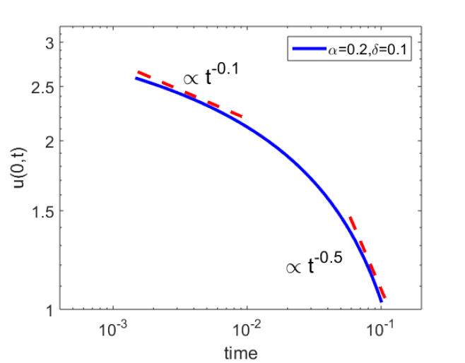
Figure 1. $u(0,t)$ of nonlocal-in-time diffusion with $\delta=0.1$, $\alpha=0.2$.

2.2. Mean square displacement (MSD)

An interesting characteristic of the diffusion process is the mean square displacement (MSD), denoted by $m(t)$ and defined by

$$m(t):=\int_{\mathbb{R}}x^{2}u(x,t)\,dx.$$

For the fundamental solution (2.1) of (1) with the kernel $\rho_{\delta}$ being a normalized PDF, i.e., (1.3) is satisfied, the corresponding $m(t)$ satisfies the nonlocal initial value problem $\mathcal{G}_{\delta}m(t)=2$ for $t>0$ with $m(t)=0$ for $t\in(-\delta,0)$. One can get that $m(t)\approx 2t$ as $t\to\infty$. Meanwhile, we have

$$m(t)\approx\frac{\sin(\alpha\pi)\delta^{1-\alpha}}{(1-\alpha)\pi}t^{\alpha}\,\quad\mbox{as}\;~{}t\to 0$$

if we use special kernels of the fractional type:

(2.2) $$\rho_{\delta}(s)=(1-\alpha)\delta^{\alpha-1}{s^{-\alpha}}.$$

Thus, we observe the transition from the sub-diffusion initially to normal diffusion at a later time.

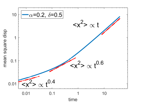
Figure 2. (a) The plot of MSD of nonlocal-in-time diffusion model (1) with $\alpha=0.2$ and $\delta=0.5$; (b) The immobile AChRs: Crossover from sub-diffusion to normal diffusion observed from the MSD curve [14, Fig. 3].

In figure 2, we plot the numerical solution of $\mathcal{G}_{\delta}m(t)=2$, i.e., the mean square displacement of the nonlocal model corresponding to $\rho_{\delta}(s)$ given by (2.2) with $\alpha=0.2$ and $\delta=0.5$. The experiment again illustrates the analytically suggested change from the early fractional anomalous diffusion regime to the later standard diffusion regime. This ”transition” or ”crossover” behavior appears in many practical applications, e.g. diffusion in lipid bilayer systems of varying chemical compositions [16, Fig. 2], and lateral motion of the acetylcholine receptors on live muscle cell membranes[14, Figs. 3, 4].

We can further study the dependence of MSD on the initial historical data. Based on the earlier discussion, we know that if the initial condition $g$ is history-independent, i.e., $g(x,t):=u_{0}(x)$, then $m(t)$, the mean square displacement of the nonlocal-in-time diffusion with a kernel function (2.2), is increasing and exhibits a weak singularity at the start, as its fractional counterpart. However, the nonlocal-in-time model (1) allows a history-dependent initial data, which will affect the growth behavior of the mean square displacement. In Fig. 3, we plot the solution of initial value problem $\mathcal{G}_{\delta}m(t)=2$, with different initial (historical) data for $t\in(-\delta,0)$:

$$g_{1}(t)=5(1+2t),\quad g_{2}(t)=\frac{1+2t}{2}\quad\mbox{and}\quad g_{2}(t)=10*\chi_{[-\delta,\delta/2]}.$$

Numerical results show that the solution $m(t)$ of initial data $g_{1}$ decays in the beginning, due to the historical-dependence of the nonlocal-in-time dynamics (where the initial data grows rapidly), and then increases at a later time, while for the initial data $g_{2}$, whose slope is smaller, we observe a strictly increasing mean square displacement function. In fact, one can prove that for initial data $k(1+2t)$, the solution $m(t)$ will keep strictly increasing when $k\leq 1$. Besides, for the step initial data $g_{3}$, the solution increases dramatically near $t=0$, and then decreases a little before its constantly linear growth. The growth behavior of $m(t)$ for different initial data is interesting and awaits further theoretical study.

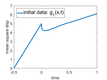
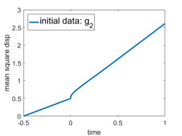
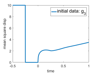
Figure 3. Mean square displacement of nonlocal-in-time model with different initial distribution, $\alpha=0.2$, $\delta=0.5$

2.3. More on the long time normal diffusion limit

The long-time normal diffusion behavior can also be observed directly from the model (1) by a simple scaling. In particular, for a typical rescaled density $\rho_{\delta}(s)=\delta^{-1}\rho_{1}(\delta^{-1}s)$ with $\rho_{1}$ being a density over the unit interval, then for $\delta_{0}$ and $v(x,t)=u(x^{\prime}.t^{\prime})$ with $x^{\prime}=x\delta_{0}^{-1/2}$ and $t^{\prime}=t\delta_{0}^{-1}$, it holds that

$$\mathcal{G}_{\delta}v(x,t) = \int_{0}^{\delta}\frac{v(x,t)-v(x,t-s)}{s}\rho_{\delta}(s)\,ds$$

$$= \frac{1}{\delta}\int_{0}^{\delta}\frac{v(x,t)-v(x,t-s)}{s}\rho_{1}(\frac{s}{\delta})\,ds$$

$$= \frac{1}{\delta}\int_{0}^{\delta}\frac{u(\frac{x}{\sqrt{\delta_{0}}},\frac{t}{\delta_{0}})-u(\frac{x}{\sqrt{\delta_{0}}},\frac{t-s}{\delta_{0}})}{s}\rho_{1}(\frac{s}{\delta})\,ds$$

$$= \frac{1}{\delta_{0}}\int_{0}^{\delta^{\prime}}\frac{u(x^{\prime},t^{\prime})-u(x^{\prime},t^{\prime}-s^{\prime})}{s^{\prime}}\rho_{\delta^{\prime}}(s^{\prime})\,ds^{\prime}$$

$$= \frac{1}{\delta_{0}}\mathcal{G}_{\delta^{\prime}}u(x^{\prime},t^{\prime}),$$

by a change of variables $\delta=\delta^{\prime}\delta_{0}$ and $s=s^{\prime}\delta_{0}$. Then, using $\Delta_{x}v(x,t)=\delta_{0}^{-1}\Delta_{x^{\prime}}v(x^{\prime},t^{\prime})$, we see that for any solution $u=u(x,t)$ of (1), the rescaled solution $v$ satisfies the same equation in the rescaled variables corresponding to a kernel with a rescaled horizon $\delta^{\prime}=\delta/\delta_{0}$. If we let $\delta_{0}\to\infty$, then the rescaled horizon $\delta^{\prime}$ goes to zero, so that $\mathcal{G}_{\delta^{\prime}}$ is effectively the conventional local time derivative. We thus see that with a diminishing memory effect, $v$ approximately satisfies the classical normal diffusion on the $O(t)$ scale, so does $u$ on the long time scale $O(t^{\prime})>>O(t)$.

For a fixed nonlocal horizon $\delta$ and at a given time $t$, one may derive the asymptotic behavior of the solution to the nonlocal-in-time model (1), as $x\rightarrow\infty$, from its Laplace transform. In particular, we have

$$\widehat{u}(x,z)\approx\frac{1}{2}c_{\delta}z^{\alpha/2-1}e^{-c_{\delta}|x|z^{\alpha/2}},\;\mbox{ as }\;z\rightarrow\infty,$$

for $c_{\delta}=\sqrt{\Gamma(2-\alpha)\delta^{\alpha-1}\alpha^{-1}}$. Hence by inverse Laplace transform, we have

$$u(x,t)\approx\frac{1}{2}c_{\delta}t^{-\alpha/2}P_{\alpha/2}(c_{\delta}x/t^{\alpha/2}),\;\mbox{ as }\;t\rightarrow 0,$$

with the Fox H function $P_{\alpha}$. This implies that $u(x,t)$ has a fractional exponential tail, i.e., for a fixed $t>0$,

$$u(x,t)\approx A_{\alpha,\delta,t}e^{-b_{\alpha,\delta,t}x^{2/(2-\alpha)}},\;\mbox{ as }\;x\rightarrow\infty.$$

2.4. Smoothing properties

Besides the patterns on statistics like MSD discussed above, another interesting feature of the nonlocal-in-time dynamics is its gradual smoothing property, namely, the solutions can become more and more smooth (as functions of the spatial variables) as time goes on. This can be derived similarly as in [11]. In fact, with the fractional kernel function in (2.2), we may see that

$$|\widetilde{u}(\xi,t)|\leq{c}/(1+b_{\delta}|\xi|^{2}t^{\alpha})$$

for any $t>0$ and some constants $c$ and $b_{\delta}$ [11, Theorem 3.2]. This implies that $|\xi|^{s}|\widetilde{u}(\xi,t)|$ is square-integrable in $(-\infty,\infty)$ only if $s<\frac{3}{2}$. This restriction reflect the limiting smoothness of the fundamental solution, i.e., the solution $u(x,t)$, for any $t>0$, has nearly $3/2$-order square integrable fractional spatial derivative and hence is only piecewise smooth. In fact, it roughly gains two more orders of differentiability with each additional $\delta$ increment in time. This observation indicates that the smoothing of the solution $u(x,t)$ takes place incrementally over time.

2.5. Comparison with fractional and normal diffusion via numerical illustrations

In Fig. 4, we plot the numerical solution of the nonlocal-in-time model with $\delta=0.2$, $\alpha=0.5$ at different time, and compare with those of the fractional diffusion and normal diffusion.

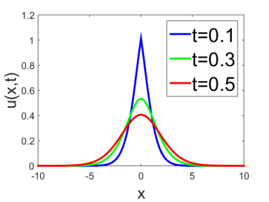
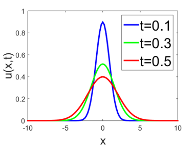
Figure 4. Left: Numerical solutions of the nonlocal-in-time diffusion equation with $\delta=0.2$, $\alpha=0.5$. Middle: Numerical solutions of the fractional diffusion with $\alpha=0.5$. Right: Numerical solutions of the local diffusion.

From numerical experiments, we observe that the solution is piecewise smooth spatially for $t\in(0,\delta)$ (the blue curve in Fig. 4(a)), and is getting more regular as $t$ keeps increasing (the green and red curves in Fig. 4(a)). This marks another distinct feature of the nonlocal-in-time model (1) with a finite memory that it has the same spatial smoothing property as the corresponding anomalous sub-diffusion (Fig. 4(b)), initially, but gets improved smoothing incrementally in time and exhibits the smoothing behavior of standard diffusion (Fig. 4(c)) as $t$ approaches infinity.

In making the above comparisons, we note that the kernel $\rho_{\delta}$ in (2.2) differs from the $\rho_{\infty}$ used for the fractional diffusion by a constant factor. Similar comparisons can be made for a rescaled kernel, and it is easy to see that, if a new kernel is taken as $\sigma\rho_{\delta}$ with a constant factor $\sigma>0$, then the fundamental solution of the nonlocal model with the new kernel is simply given by $u(x/\sqrt{\sigma},t)$ with $u(x,t)$ being the fundamental solution of (1) with the original kernel.

(a) t=0.1

(b) t=0.5

(c) t=0.1

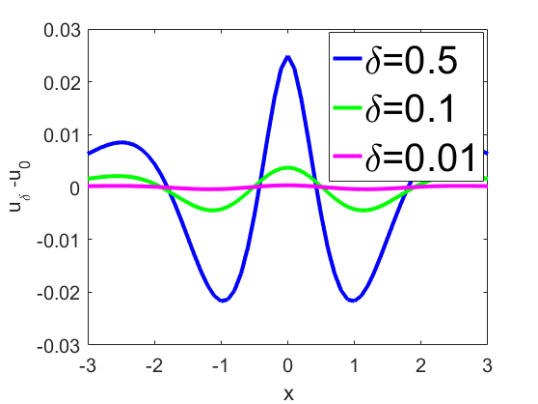
(d) t=0.5

Figure 5. Figures (a) and (b): The plot of numerical solutions of nonlocal-in-time diffusion at $t=0.1$, $0.5$ with $\alpha=0.5$ and different nonlocal horizons. Figures (c) and (d): The plot of difference between solutions of nonlocal diffusion with different nonlocal horizons and the solution of local diffusion.

It is interesting to numerically study the local limit of the nonlocal-in-time model that has been rigorously established in [11]. In Fig. 5, we plot the numerical solutions of nonlocal-in-time model with different nonlocal horizons at $t=0.1$ and $0.5$, as well as the difference between the nonlocal solutions and the local one. It can be observed that as $\delta$ goes to zero, the solution of the nonlocal diffusion model converges to the solution of the local one.

2.6. Nonlocal-in-time dynamics on a finite spatial domain

To complement the study on the infinite one dimensional spatial domain, we now briefly turn to the nonlocal-in-time parabolic equation (1) in a bounded domain with a homogeneous Dirichlet boundary condition. Specifically, we consider the following initial-boundary value problem for $u=u(x,t)$:

$$\mathcal{G}_{\delta}u(x,t)-\Delta u(x,t)=0, \quad\mbox{in}~{}~{}\Omega\times[0,T],$$

(2.3) $$u(x,t)=0, \quad\mbox{in}~{}~{}\partial\Omega\times[0,T],$$

$$u(x,t)=g(x,t), \quad\mbox{in}~{}~{}\Omega\times[-\delta,0),$$

where $\Omega$ is a bounded convex polyhedral domain in $\mathbb{R}^{d}$ $(d\geq 1)$ with a boundary $\partial\Omega$. Mathematical studies of (2.6) such as well-posedness and numerical analysis can be found in [11].

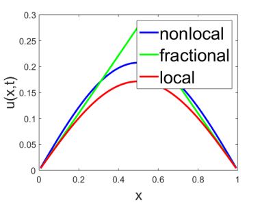
Figure 6. Numerical solutions of local, fractional and nonlocal diffusion models, $\delta=0.1$ and $\alpha=0.5$.

To illustrate our findings, we use the fractional kernel given by (2.2) and compare its solution behavior with those of fractional diffusion and local diffusion. In Fig. 6, we present a numerical solution of an 1-D nonlocal model (2.6) on $\Omega=(0,1)$ at different time $t=0.05$, $0.15$ and $0.25$ with $\delta=0.1$ and $\alpha=0.5$, The initial (historical) data is taken as a Dirac-delta measure at $x=1/2$. We can observe that the nonlocal diffusion gradually regularize the solution as $t\rightarrow\infty$. Moreover, the fractional diffusion decays fastest for small $t$, and the classical local diffusion decays fastest for large $t$, while nonlocal diffusion exhibits an intermediate behavior.

(a) nonlocal, $t=0.01$

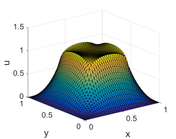
(b) fractional, $t=0.01$

(c) standard, $t=0.01$

(d) nonlocal, $t=1.1$

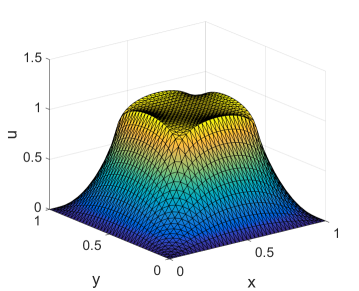
(e) fractional, $t=1.1$

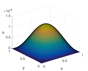
(f) local, $t=1.1$

Figure 7. Numerical solutions of local, fractional and nonlocal models with $\Omega=(0,1)^{2}$, $\delta=1$ and $\alpha=0.5$ at different time.

Next, we show a two-dimensional example with $\Omega=(0,1)^{2}$ and an initial data given by the Dirac-delta measure concentrated on the boundary of a smaller square $[\frac{1}{4},\frac{3}{4}]\times[\frac{1}{4},\frac{3}{4}]$. Comparisons with the corresponding solutions of the fractional and local diffusion models are all provided.

3. Additional discussions on nonlocal-in-time models

As we can see from the examples presented in this paper, the nonlocal-in-time model (1) is a simple modification of the traditional dynamic systems where the instant rate of change ($\partial_{t}u$) is replaced by a nonlocal rate of change $(\mathcal{G}_{\delta}u)$. The local limit, i.e., the standard derivative, is simply the extreme case where the kernel function $\rho_{\delta}(s)$ degenerates into a singular point measure at $s=0$. On the other hand, we have also mentioned that by picking suitable fractional type kernels with $\delta\rightarrow\infty$, the nonlocal-in-time model can recover fractional differential equations as well. We thus advocate the equation (1) as a more general model, whose mathematical theory (such as existence, uniqueness and regularity of solutions), along with numerical analysis of some discrete approximations, can be found in [11].

There have been a large number of studies on time-fractional dynamics, which are used to model the continuous time random walk of particles in heterogeneous media [23, 3, 24]. The fractional derivative arising in fractional sub-diffusion model results from a fractional power-law type waiting time probability. However, such specific choices of memory kernels are rather restrictive. One may argue that perhaps there remains a lack of compelling evidence that the nature is confined by such limited forms of kernels. For example, let us consider the situation where particles may explore some environment that is a kind of labyrinthine (bearing short-time sub-diffusion) but homogenizes on large length scales (resulting in a long-time normal diffusion). In recent experimental studies of such systems, there have been a number reports on different diffusion regimes from short-time sub-diffusion to long-time normal diffusion [16, 14]. This motivates us to look for a simple and effective model to capture the transient dynamics. Naturally, there may be different mathematical models for such crossover phenomena. For example, besides the recently proposed diffusing diffusivity model (cf. [4, 13, 15]), a variable-order fractional diffusion equation

$$\partial_{t}^{\alpha(t)}u-\Delta u=0$$

has been used in [28] with a time-dependent order $\alpha(t)$. However, analyzing such model (theoretically or numerically) remains a difficult task from a mathematical perspective, besides the challenge for further physical validation.

In contrast, the nonlocal-in-time model (1) with a constant finite history dependence leads to a more direct and intuitive way to interpret and to capture the crossover behavior. Moreover, although different models may produce similar behavior on MSD, other statistics and spatial/temporal patterns of the solutions may differ [22, 27]. Thus, it is important to conduct more mathematical investigations and numerical simulations, like the studies presented here, in order to provide a deeper understanding of the underlying process.

From a modeling perspective, the nonlocal-in-time model (1) can also be explained by a model of random walk with trapping. For a truncated fractional kernel function of the type (1.4), the probability intensity of the trapping event is related to $c_{\alpha}s^{-\alpha-1}\chi_{(0,\delta)}=:\rho_{\delta}(s)/s$. As an illustration, let us focus on a simple 1-D case. First, in discrete time steps with a uniform step size $\tau$, a random walker is assumed to stay in its current position, or move to one of its nearest neighbor sites with length $h$ and in a random left or right direction. Let $u(x,t)$ be the probability that the walker appears at position $x$ and time $t$, and $\eta(x,t)$ be the probability that the walker has just arrived at $x$ and $t$. By assuming that the maximal waiting time is $\delta$, we then get

(3.1) $$u(x,t)=\sum_{k=1}^{\delta/\tau}\omega_{k}\eta(x,t-k\tau)+\eta(x,t),$$

where $\omega_{k}$ is the probability that the walker waits for at least $k\tau$ after arriving at a position. We let $p_{k}$ be the probability that the walker stops exactly $k\tau$ after its arrival, which for $k=1,2,...,\delta/\tau$, is assumed to be of the form:

$$p_{k-1}=\Big{(}\frac{1}{k\tau}\int_{(k-1)\tau}^{k\tau}s^{-\alpha}\,ds\Big{)}/\Big{(}\sum_{k=1}^{\delta/\tau}\frac{1}{k\tau}\int_{(k-1)\tau}^{k\tau}s^{-\alpha}\,ds\Big{)}.$$

Then, it is obvious that

$$\omega_{k}=1-\sum_{i=0}^{k-1}p_{k}.$$

The discrete model of random walk with trapping gives that for $h$ small,

$$\eta(x,t) =\sum_{k=1}^{\delta/\tau}\frac{1}{2}(\eta(x-h,t-k\tau)+\eta(x+h,t-k\tau))p_{k-1}$$

$$\approx\sum_{k=1}^{\delta/\tau}(\eta(x,t-k\tau)+\frac{h^{2}}{2}\eta_{xx}(x,t-k\tau))p_{k-1}.$$

Let $\mathcal{G}_{\delta}^{\tau}$ be defined by

$$\mathcal{G}_{\delta}^{\tau}u(t) =u(t)\Big{(}\sum_{k=1}^{\delta/\tau}\frac{1}{k\tau}\int_{(k-1)\tau}^{k\tau}\rho_{\delta}(s)\,ds\Big{)}-\sum_{k=1}^{\delta/\tau}\frac{u(t-k\tau)}{k\tau}\int_{(k-1)\tau}^{k\tau}\rho_{\delta}(s)\,ds,$$

with $\rho_{\delta}(s)=(1-\alpha)\delta^{\alpha-1}s^{-\alpha}$. Then a simple calculation yields that $\mathcal{G}_{\delta}^{\tau}u(t)\approx\mathcal{G}_{\delta}u(t)$ for small $\tau$, and for

$$c_{\delta,\alpha}=(1-\alpha)\delta^{\alpha-1}\sum_{k=1}^{\infty}\frac{1}{k}\int_{k-1}^{k}s^{-\alpha}\,ds$$

we can get

$$\sum_{k=1}^{\delta/\tau}\frac{1}{k\tau}\int_{(k-1)\tau}^{k\tau}\rho_{\delta}(s)\,ds\approx c_{\delta,\alpha}\tau^{-\alpha}.$$

Therefore, we observe that for for small $\tau^{\alpha}\approx h^{2}$,

(3.2) $$\mathcal{G}_{\delta}^{\tau}\eta(x,t)-\frac{c_{\delta,\alpha}}{2}\frac{h^{2}}{\tau^{\alpha}}\eta_{xx}(x,t)=0.$$

The nonlocal-in-time model (1) also follows from (3.2) by applying $\mathcal{G}_{\delta}^{\tau}$ on the equation (3.1), using (3.2) and letting $\tau^{\alpha}\approx h^{2}\rightarrow 0$.

To substantiate this stochastic explanation, we compared numerical solution of (3.2) computed by finite different method with the Monte-Carlo solution using the particle method, in Fig. 8. We consider the infinite domain in one space dimension $\Omega=\mathbb{R}$, and let the initial (historical) data be the Dirac-delta measure concentrated at $x=0$ i.e., we only track the movement of a single particle, starting from the position $x=0$. Numerical results indicate that the Monte-Carlo solution fits the finite difference solution very well, and this supports our theoretical results.

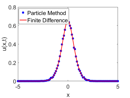
Figure 8. Numerical solutions of the nonlocal-in-time diffusion equation with $\delta=0.2$, $\alpha=0.75$ and Dirac-Delta initial condition, at $t=0.1$, $0.2$, $0.3$ and $0.4$, respectively.

4. Conclusion

In conclusion, through the computation of solutions and their statistics such as the mean square displacement, and through the comparisons of them with the local and fractional counterparts, this paper shows that the nonlocal-in-time diffusion with a finite memory can be a very effective model that provides an intermediate case between normal and fractional diffusions and can serve to describe effectively various processes involving crossovers of different diffusion regimes. The model is showing promises in capturing experimental observations of diffusion in heterogeneous media without introducing complications and heterogeneities in the model themselves. The essence lies in the finite memory effect and how it compares with the overall dynamic history. One may naturally ask how the memory kernel and the horizon should be chosen, which becomes an interesting inverse problem to be further investigated. Other interesting issues to be studied include the connection to other models of anomalous diffusion such as those discussed in the above and in section 1 and the replacement of normal diffusion operator (the Laplacian $\Delta$) by nonlocal diffusion operators in the spatial directions. The latter is often associated with super-diffusion [7, 5], so that a combined nonlocal in time and space diffusion model might effectively describe sub-, normal- and super-diffusion regimes.

References

- [1] M. Allen, L. Caffarelli, and A. Vasseur. A parabolic problem with a fractional time derivative. Archive for Rational Mechanics and Analysis, 221(2):603–630, 2016.
- [2] A. M. Berezhkovskii, L. Dagdug, and S. M. Bezrukov. Discriminating between anomalous diffusion and transient behavior in microheterogeneous environments. Biophysical Journal, 106(2):L9–L11, 2014.
- [3] B. Berkowitz, J. Klafter, R. Metzler, and H. Scher. Physical pictures of transport in heterogeneous media: Advection-dispersion, random-walk, and fractional derivative formulations. Water Resources Research, 38(10):9–1, 2002.
- [4] M. V. Chubynsky and G. W. Slater. Diffusing diffusivity: a model for anomalous, yet brownian, diffusion. Physical review letters, 113(9):098302, 2014.
- [5] O. Defterli, M. D Elia, Q. Du, M. Gunzburger, R. Lehoucq, and M. M. Meerschaert. Fractional diffusion on bounded domains. Fractional Calculus and Applied Analysis, 18(2):342–360, 2015.
- [6] Q. Du, M. Gunzburger, R. Lehoucq, and K. Zhou. A nonlocal vector calculus, nonlocal volume-constrained problems, and nonlocal balance laws. Mathematical Models and Methods in Applied Sciences, 23(3):493–540, 2013.
- [7] Q. Du, M. Gunzburger, R. B. Lehoucq, and K. Zhou. Analysis and approximation of nonlocal diffusion problems with volume constraints. SIAM Review, 54(4):667–696, 2012.
- [8] Q. Du, Y. Tao, X. Tian, and J. Yang. Robust a posteriori stress analysis for quadrature collocation approximations of nonlocal models via nonlocal gradients. Comp Meth. Applied Mech. Eng., 310:605–627, 2016.
- [9] Q. Du, L. Toniazzi, and Z. Zhou. Stochastic representation of solution to nonlocal-in-time diffusion. Stochastic Processes and their Applications, 2019.
- [10] Q. Du, L. Toniazzi, and Z. Zhou. Stochastic representation of solution to nonlocal-in-time diffusion. Stochastic Processes and their Applications, 2019.
- [11] Q. Du, J. Yang, and Z. Zhou. Analysis of a nonlocal-in-time parabolic equation. Discrete and Continuous Dynamical Systems - Series B, 22, 2017.
- [12] W. Feller. An Introduction to Probability Theory and its Applications, volume 2. John Wiley & Sons, 2008.
- [13] D. S. Grebenkov. A unifying approach to first-passage time distributions in diffusing diffusivity and switching diffusion models. Journal of Physics A: Mathematical and Theoretical, 52(17):174001, 2019.
- [14] W. He, H. Song, Y. Su, L. Geng, B. Ackerson, H. Peng, and P. Tong. Dynamic heterogeneity and non-Gaussian statistics for acetylcholine receptors on live cell membrane. Nature communications, 7, 2016.
- [15] R. Jain and K. Sebastian. Diffusing diffusivity: a new derivation and comparison with simulations. Journal of Chemical Sciences, 129(7):929–937, 2017.
- [16] J.-H. Jeon, H. M.-S. Monne, M. Javanainen, and R. Metzler. Anomalous diffusion of phospholipids and cholesterols in a lipid bilayer and its origins. Physical Review Letters, 109(18):188103, 2012.
- [17] A. Kilbas, H. Srivastava, and J. Trujillo. Theory and Applications of Fractional Differential Equations. Elsevier, Amsterdam, 2006.
- [18] N. Korabel and E. Barkai. Paradoxes of subdiffusive infiltration in disordered systems. Physical Review Letters, 104(17):170603, 2010.
- [19] F. Mainardi, Y. Luchko, and G. Pagnini. The fundamental solution of the space-time fractional diffusion equation. Fractional Calculus and Applied Analysis, 4(2):153–192, 2001.
- [20] S. A. McKinley, L. Yao, and M. G. Forest. Transient anomalous diffusion of tracer particles in soft matter. Journal of Rheology, 53(6):1487–1506, 2009.
- [21] T. Mengesha and Q. Du. Characterization of function spaces of vector fields and an application in nonlinear peridynamics. Nonlinear Analysis A: Theory, Methods and Applications, 140:82–111, 2016.
- [22] R. Metzler. Brownian motion and beyond: first-passage, power spectrum, non-gaussianity, and anomalous diffusion. arXiv preprint arXiv:1908.06233, 2019.
- [23] R. Metzler and J. Klafter. The random walk’s guide to anomalous diffusion: a fractional dynamics approach. Physics Reports, 339(1):1–77, 2000.
- [24] R. Metzler and J. Klafter. The restaurant at the end of the random walk: recent developments in the description of anomalous transport by fractional dynamics. Journal of Physics A: Mathematical and General, 37(31):R161, 2004.
- [25] M. J. Saxton. Wanted: a positive control for anomalous subdiffusion. Biophysical Journal, 103(12):2411–2422, 2012.
- [26] I. M. Sokolov. Models of anomalous diffusion in crowded environments. Soft Matter, 8(35):9043–9052, 2012.
- [27] V. Sposini, A. V. Chechkin, F. Seno, G. Pagnini, and R. Metzler. Random diffusivity from stochastic equations: comparison of two models for brownian yet non-gaussian diffusion. New Journal of Physics, 20(4):043044, 2018.
- [28] H. Sun, Z. Li, Y. Zhang, and W. Chen. Fractional and fractal derivative models for transient anomalous diffusion: Model comparison. Chaos, Solitons and Fractals, 102:346–353, 2017.