Periodic event-triggered output regulation for linear multi-agent systems
Extended version (Supplementary file)

Abstract

This study considers the problem of periodic event-triggered (PET) cooperative output regulation for a class of linear multi-agent systems. The advantage of the PET output regulation is that the data transmission and triggered condition are only needed to be monitored at discrete sampling instants. It is assumed that only a small number of agents can have access to the system matrix and states of the leader. Meanwhile, the PET mechanism is considered not only in the communication between various agents, but also in the sensor-to-controller and controller-to-actuator transmission channels for each agent. The above problem set-up will bring some challenges to the controller design and stability analysis. Based on a novel PET distributed observer, a PET dynamic output feedback control method is developed for each follower. Compared with the existing works, our method can naturally exclude the Zeno behavior, and the inter-event time becomes multiples of the sampling period. Furthermore, for every follower, the minimum inter-event time can be determined a prior, and computed directly without the knowledge of the leader information. An example is given to verify and illustrate the effectiveness of the new design scheme.

1 Introduction

Cooperative control for multi-agent systems has attracted extensive attention because of its potential applications (Yang, Zhang, Feng, Yan, & Wang, 2019; Shi, & Shen, 2017; Liu, & Huang, 2019; Li, Xing, Zhao, & Shi, 2017; Singh, Tiwari, Garg, 2018; Zhu, Zheng, & Zhou, 2019) in multi-vehicle formation, wireless sensor network, electrical power systems $etc$. The cooperative control problem includes leaderless and leader-following consensus, containment, rendezvous, formation $etc$. Various control strategies have been utilized for multi-agent systems, such as adaptive control (Li, Qu, & Tong, 2019; Shi, & Shen, 2017; Zheng, Shi, Wang, & Shi, 2019; Xu, Yang, Wang, & Shu, 2019), sliding mode control (Sun, Hu, Xie, & Egerstedt, 2018) and model predictive control.

The output regulation problem for multi-agent systems has recently drawn much interest from researchers. The purpose of the regulation problem is to make the output of each follower track a class of reference input and simultaneously handle the external disturbance (Chen, & Huang, 2015). The reference input and disturbance signals are generated by the exosystem or leader. In this sense, the output regulation problem is more general than the standard tracking or stabilization problem (Chen, & Sun, 2020; Li, Li, & Tong, 2019; Xing, Wen, Liu, Su, & Cai, 2017; Zhu, & Zheng, 2019). Until now, many excellent results have been proposed in this field (Bin, Marconi, & Teel, 2019; Chen, & Chen, 2017; Chen, & Huang, 2015; Liu, & Huang, 2020; Yang, Zhang, Feng, Yan, & Wang, 2019). For instance, in Cai, Lewis, Hu, & Huang (2017), based on a new adaptive distributed observer, the cooperative output regulation problem for linear multi-agent systems was solved. Su (2019) studied the semi-global output feedback regulation problem for a class of nonlinear multi-agent systems with heterogeneous relative degrees.

Most of the above works attempt to solve the output regulation problem under the assumption that all the states can be transmitted continuously. However, continuous transmission can entail high communication cost and energy consumption. As a solution to this issue, event-triggered control strategies have been presented (Cheng, & Ugrinovskii, 2016; Hu, Liu, & Feng, 2018, 2019; Yang, Zhang, Feng, Yan, & Wang, 2019). The idea of event-triggered control is to transmit the data according to a well-defined triggered condition. In this way, the communication burden can be reduced considerably.

Different types of event-triggered mechanisms (Nowzari, Garcia, & Cortés, 2019) have been proposed such as continuous-time event-triggered control, self-triggered control, dynamic event-triggered control $etc$. More recently, the periodic event-triggered (PET) control strategy has become a hot topic (Behera, Bandyopadhyay, & Yu, 2018; Meng, Xie, & Soh, 2017; Wang, Postoyan, Nesic, & Heemels, 2019; Yang, Sun, Zheng, & Li, 2018). Compared with other event-triggered mechanisms, the key feature of PET control is that the data transmission and the triggered condition are only needed to be monitored at discrete sampling instants. This feature benefits control systems in the following aspects: 1) It naturally rules out the Zeno behavior; 2) The inter-event times become multiples of the sampling period. This can be very helpful for digital implementation, and scheduling of many applications on a shared communication medium; 3) It is more practical in some engineering situations where the states measurements are only available at periodic intervals due to the constraints on sensors and network. 4) It can reduce the energy consumption for evaluating triggered conditions in contrast with continuous-time event-triggered control. Nevertheless, to the best of our knowledge, no works have ever considered the periodic event-triggered output regulation for multi-agent systems.

Motivated by the aforementioned idea, this paper will consider the PET cooperative output regulation problem for a class of linear multi-agent systems. The problem is challenging due to the following reasons: 1) Only some of the followers have access to the system matrix or the states information of the leader; 2) The PET mechanism is considered not only in the communication between various agents, but also in the sensor-to-controller and controller-to-actuator transmission channels for each agent; 3) Only the output information of the followers is available for the controller design.

The above problem set up makes the existing output regulation methods (Chen, & Huang, 2015; Deng, & Yang, 2019) infeasible. Moreover, directly extending the distributed observer method (Cai, & Hu, 2019; Cai, & Huang, 2016; Cai, Lewis, Hu, & Huang, 2017; Liu, & Huang, 2019) to our case is not easy because of the PET mechanism. In fact, PET control is more general than sampled data control. However, the sampled data output regulation problem has not been fully investigated so far, not to mention PET output regulation. This research gap makes stability analysis challenging.

Our work provides the following main contributions:

• Novel PET distributed observers are formulated to estimate the system matrix and state information of the leader;

• Using the estimated leader information, a new PET dynamic output feedback controller is designed for each follower;

• Based on the skillful use of some matrix norm and Gronwall’s inequalities, we prove that the cooperative output regulation problem is solvable by the proposed method.

• For each follower, the minimum inter-event time can be determined a prior and computed directly without the knowledge of the leader information. Moreover, by decreasing the gains of the distributed observer, the minimum inter-event time for the communication between various agents can be made arbitrary long.

The organization of the paper is as follows. Problem formulation and preliminaries are given in Section 2. The proposed PET distributed observer and output feedback controller are presented in Section 3. Simulations are conducted and presented in Section 4. Section 5 concludes the paper.

Notations. Given a matrix $X_{i}\in\mathbb{R}^{n_{i}\times m}(i=1,2,...,N)$, $\mathrm{col}(X_{1},X_{2},...,X_{N})=[X_{1}^{\mathrm{T}}\thinspace X_{2}^{\mathrm{T}}\thinspace...X_{N}^{\mathrm{T}}]^{\mathrm{T}}$. For $A\in\mathbb{R}^{n\times m}$, $\mathrm{vec}(A)=\mathrm{col}(A_{1},A_{2},...,A_{m})$ where $A_{i}\in\mathbb{R}^{n}$ denotes the $i$th column of $A$. $||A||,||A||_{F}$ are the $2$-norm and Frobenius-norm of matrix $A$.

2 Problem formulation and preliminaries

2.1 Problem formulation

Consider a multi-agent system consisting of $N$ followers and $1$ leader. The dynamic of the leader is given by:

$$\dot{v} =Sv$$ (1)

where $v\in\mathbb{R}^{n_{v}}$ is the reference input and/or external disturbance with a positive integer $n_{v}$. $S$ is a given system matrix.

The followers are given by the following linear system:

$$\dot{x}_{i} =A_{i}x_{i}+B_{i}u_{i}+E_{i}v,$$ (2)

$$e_{i} =C_{i}x_{i}+D_{i}u_{i}+F_{i}v,$$ (3)

$$y_{mi} =C_{mi}x_{i}+D_{mi}u_{i}+F_{mi}v$$ (4)

where $i\in\{1,2,...,N\}$. $x_{i}\in\mathbb{R}^{n_{i}}$, $u_{i}\in\mathbb{R}^{n_{ui}}$, $e_{i}\in\mathbb{R}^{n_{ei}}$, $y_{mi}\in\mathbb{R}^{n_{yi}}$ are the system states, control effort, consensus error and measurement output respectively with positive integers $n_{i},n_{ui},n_{ei},n_{yi}$. $A_{i},B_{i},C_{i},D_{i},E_{i},F_{i},C_{mi},D_{mi},F_{mi}$ are the given system matrices.

The communication for the multi-agent systems is represented by a directed graph $\mathcal{G}$. Let $\mathcal{G}=(\mathcal{V},\mathcal{E})$ where $\mathcal{V}=\{1,2,...,N\}$ denotes the set of vertices, $\mathcal{E}\subseteq\mathcal{V}\times\mathcal{V}$ the set of edges. Let $\mathcal{N}_{i}$ represents the neighbors of agent $i$, $i.e.$, $\mathcal{N}_{i}=\{j|j\in\mathcal{V}|(j,i)\in\mathcal{E}\}$. Define matrix $\mathcal{W}=[a_{ij}]\in\mathbb{R}^{N\times N}$ such that if $(j,i)\in\mathcal{E}$ then $a_{ij}=1$, otherwise $a_{ij}=0$. Self-loop is not allowed, $i.e.$, $a_{ii}=0$ for $i\in\mathcal{V}$. Define Laplacian matrix as $\mathcal{L}=\mathcal{D}-\mathcal{\mathcal{W}}$ with $\mathcal{D}=\mathrm{diag}(d_{1},d_{2},...,d_{N})$ and $d_{i}=\sum_{j\in\mathcal{N}_{i}}a_{ij}(i\in\mathcal{V})$. For the information transmission between the leader and followers, define $a_{i0}$ such that if the followers are connected to the leader, then $a_{i0}=1$; otherwise $a_{i0}=0$. Also let $a_{0i}=0$. Note that only a small portion of followers have access to the leader.

Based on the above analysis, the cooperative output regulation problem is formulated as follows:

Problem 1.

Given a multi-agent system (1)-(3) with its corresponding graph $\mathcal{G}$, develop a PET distributed control law for each follower such that

1) All the closed loop signals are bounded for all $t\in[0,+\infty)$; and,

2) The output regulation error satisfies $\underset{t\rightarrow+\infty}{\lim}||e_{i}(t)||=0$ or $\underset{t\rightarrow+\infty}{\lim}||e_{i}(t)||\leq\varLambda_{i}$ for $i\in\{1,2,...,N\}$ where $\varLambda_{i}$ is a small positive constant.

Remark 1.

As we will see in Section 3, according to whether the PET mechanism is adopted for the controller-to-actuator channel, the cooperative output regulation error will be regulated to exact zero or a small neighborhood around the origin. In addition, when the limitation of $||e_{i}(t)||$ does not exist, $\underset{t\rightarrow+\infty}{\lim}||e_{i}(t)||$ should be understood as $\underset{t\rightarrow+\infty}{\lim\sup}||e_{i}(t)||$.

Remark 2.

The regulation error in (3) can be seen as a generalization of the consensus error defined in many literatures (Deng, & Yang, 2019). For instance, suppose the output of the followers is $y_{i}=C_{i}x_{i}$. Then if one wants the followers to track the leader, the consensus error may be defined as $y_{i}-v=C_{i}x_{i}-v$. This is equivalent to let $D_{i}=0,F_{i}=-I$ in (3). In addition, note that the measurement output $y_{mi}$ in (4) may not equal to the real output of the followers. For example, if the real output of the followers is $y_{i}=C_{mi}x_{i}+D_{mi}u_{i}$., then the measurement output $y_{mi}$ in (4) indicates that the real output $y_{i}$ may be influenced by an external disturbance $F_{mi}v$ where $v$ is generated by the exosystem $v=Sv$.

2.2 Preliminaries

In this subsection, we will introduce some basic assumptions and results for the cooperative output regulation problem. It is divided into three parts.

1) Graph and leader

For the communication graph, we assume that:

Assumption 1.

The graph containing the leader and $N$ followers has a directed spanning tree with the leader as the root.

Then we have the following result.

Lemma 1.

(Cai, Lewis, Hu, & Huang, 2017) Under Assumption 1, $-\mathcal{H}$ is a Hurwitz matrix with $\mathcal{H}\triangleq\mathcal{L}+\mathcal{B}$ and $\mathcal{B}\triangleq\mathrm{diag}(a_{10},a_{20},...,a_{N0})$.

For the leader (1), we assume

Assumption 2.

The leader system is neutrally stable, i.e., the eigenvalues of $S$ are semi-simple with zero real parts.

Remark 3.

Under the above assumption, we know that as long as the initial value $v(0)$ is bounded, $v(t)$ is bounded on $[0,+\infty)$. Meanwhile, a wide class of signals, such as sine and step signals, can be generated by the leader system (1). In addition, from Cai, & Huang (2016), without loss of generality $S$ can be selected to be a skew-symmetric matrix such that $S^{T}=-S$.

2) Followers

For linear system (3), we make the following assumptions.

Assumption 3.

For $i=1,2,...,N$, the system matrices satisfy:

1) $(A_{i},B_{i})$ are stabilizable;

2) $(C_{mi},A_{i})$ are detectable;

3) The following linear matrix equations admit a solution $(X_{i},U_{i})$

$$X_{i}S =A_{i}X_{i}+B_{i}U_{i}+E_{i},$$

$$0 =C_{i}X_{i}+D_{i}U_{i}+F_{i}.$$ (5)

The above assumptions are standard in output regulation theory. Meanwhile, from Cai, Lewis, Hu, & Huang (2017), we know the solution $(X_{i},U_{i})$ can be solved adaptively. We briefly explain the idea as follows. Let $\chi_{i}=\mathrm{vec}(\mathrm{col}(X_{i},U_{i}))$, $\beta_{i}=\mathrm{vec}(\mathrm{col}(E_{i},F_{i}))$,

$$\mathcal{A}_{i}=S^{T}\varotimes\left[\begin{array}[]{cc}I&0\\ 0&0\end{array}\right]-I\varotimes\left[\begin{array}[]{cc}A_{i}&B_{i}\\ C_{i}&D_{i}\end{array}\right],$$

$$\hat{\mathcal{A}}_{i}(t)=\hat{S}_{i}^{T}(t)\varotimes\left[\begin{array}[]{cc}I&0\\ 0&0\end{array}\right]-I\varotimes\left[\begin{array}[]{cc}A_{i}&B_{i}\\ C_{i}&D_{i}\end{array}\right]$$

where $\hat{\mathcal{A}}_{i}(t),\hat{S}_{i}(t)$ are time-varying matrices.

Then (5) can be written as:

$$\mathcal{A}_{i}\chi_{i}=\beta_{i}.$$

Define $\hat{\chi}_{i}$ with the adaptive law

$$\dot{\hat{\chi}}_{i}=-\kappa\hat{\mathcal{A}}_{i}^{T}(\hat{\mathcal{A}_{i}}\hat{\chi}_{i}-\beta_{i})$$ (6)

where $\kappa>0$ is a positive design parameter.

Meanwhile, define the adaptive solution $\hat{X}_{i},\hat{U}_{i}$ such that they have the same dimensions as $X_{i},U_{i}$ and

$$\mathrm{vec}(\mathrm{col}(\hat{X}_{i},\hat{U}_{i}))=\hat{\chi}_{i}.$$ (7)

Then we have the following result (Cai, Lewis, Hu, & Huang, 2017).

Lemma 2.

If $S-\hat{S}_{i}$ converges to zero exponentially, $\chi_{i}-\hat{\chi}_{i}$ and $X_{i}-\hat{X}_{i},U_{i}-\hat{U}_{i}$ will all converge to zero exponentially.

3) Useful inequalities

Finally, we introduce some inequalities which will be used in the stability analysis.

Lemma 3.

(Matrix norm inequalities) Given matrices $A,B\in\mathbb{R}^{n\times n}$, we have

1) $||\mathrm{e}^{A+B}-\mathrm{e}^{A}||\leq\mathrm{e}^{||A||+||B||}||B||$;

2) $||A||\leq||A||_{F}\leq\sqrt{n}||A||$;

3) $||\mathrm{e}^{A}||\leq\mathrm{e}^{||A||}$.

Proof.

1) is from Lemma 1 in Yang, & Liberzon (2018). 2) and 3) can be proved using basic matrix theory. ∎

Lemma 4.

(Gronwall’s inequality) Given a real-valued function $w(t):[0,+\infty)\rightarrow\mathbb{R}$ such that

$$w(t)\leq\alpha+\int_{t_{0}}^{t}\beta w(\tau)d\tau$$

for $\forall t\in[t_{0},+\infty)$ where $\alpha,\beta,t_{0}>0$ are positive constants. Then

$$w(t)\leq\alpha\mathrm{e}^{\beta(t-t_{0})}.$$

3 Main results

In this section, we will discuss the output regulation problem for linear multi-agent systems by (1)-(3). The control scheme is shown in Fig. 1. For the communication between various agents, the controller of agent $i$ will send/receive the information to/from its neighbors based on the PET Mechanism A (PETM-A). For the sensor-to-controller channel, the sensor will sample the output information from the plant and transmit it to the controller by the PET Mechanism B (PETM-B). For the controller-to-actuator channel, two different situations will be considered. We will first consider the situation where the transmission is continuous, $i.e.$, the switch in Fig. 1 is on node 1. Then, we will consider the case when the switch is on node 2, that is the control signal will be transmitted to the actuator based on the PET Mechanism C (PETM-C). We can see that the PET mechanisms are not only used for the communication between various agents, but also for the sensor-to-controller and controller-to-actuator channel in each agent.

The proposed controller is composed of two parts: a PET distributed observer and a PET control law. The PET distributed observer is used to estimate the system matrix $S$ and $v$ of the leader based on PETM-A. The control law will use the estimated information to generate the control signal according to PETM-B and PETM-C.

Next, we will explain these two parts respectively.

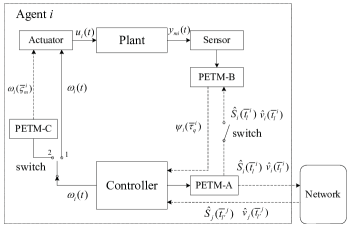
Figure 1: Control scheme.

Remark 4.

Notably the above control scheme indicates that the PET mechanism is considered not only in the communication between various agents, but also in the sensor-to-controller and controller-to-actuator transmission channels for each agent. The motivation for considering this control scheme is that in some situations the control of a single agent may require the network communication between the controller and the sensor/actuator. A number of applications may involve the formation control of unmanned automobiles where control of each automobile is based on network (Zhang, Gao, & Kaynak, 2013), the networked control of a group of UAVs based on remote controllers/ground bases (Cuenca, Antunes, Castillo, Garcia, Khashooei, & Heemels, 2019; Liu, Ma, Lewis, & Wan, 2019), the cooperative control of robot manipulators $etc$.

3.1 PET distributed observer

Let $0=t_{0}<t_{1}<\cdots<t_{k}<\cdots$ denote the sampling time instants for the multi-agent systems where $t_{k}\triangleq kT$ and $T>0$ is the sampling period. Also define set $\Omega_{T}=\{t_{0},t_{1},...,t_{k},...\}.$ On each time interval $[t_{k},t_{k+1})$, the distributed observer for agent $i(i=1,2,...,N)$ is designed as:

$$\dot{\hat{S}}_{i} =\mu_{1}\sum_{j=0}^{N}a_{ij}(\hat{S}_{j}(\overline{t}_{l^{\prime}}^{j})-\hat{S}_{i}(\overline{t}_{l}^{i})),$$ (8)

$$\dot{\hat{v}}_{i} =\hat{S}_{i}(\overline{t}_{l}^{i})\hat{v}_{i}(t)+\mu_{2}\sum_{j=0}^{N}a_{ij}(\overline{v}_{j}(t,\overline{t}_{l^{\prime}}^{j})-\overline{v}_{i}(t,\overline{t}_{l}^{i}))$$ (9)

where $\mu_{1},\mu_{2}>0$ are two positive parameters. $\hat{S}_{0}(t)\equiv S$,

$$\overline{v}_{i}(t,\overline{t}_{l}^{i})=\mathrm{e}^{\hat{S}_{i}(\overline{t}_{l}^{i})(t-\overline{t}_{l}^{i})}\hat{v}_{i}(\overline{t}_{l}^{i})(i=1,...,N)$$ (10)

and $\hat{v}_{0}(t)\triangleq v$, $\overline{v}_{0}(t,t_{l}^{0})\triangleq\mathrm{e}^{S(t-t_{l}^{0})}\hat{v}_{0}(t_{l}^{0})=v(t)$.

Note that $0=\overline{t}_{0}^{i}<\overline{t}_{1}^{i}<\cdots<\overline{t}_{l}^{i}<\cdots$ denote the event-triggered time instants. On time instant $\overline{t}_{l}^{i}$, agent $i$ will send $\hat{S}_{i}(\overline{t}_{l}^{i})$ and $\hat{v}_{i}(\overline{t}_{l}^{i})$ to its neighbors. The event-triggered time instants are determined by PETM-A in Fig. 1 which is given by:

$$\overline{t}_{l+1}^{i}=\mathrm{inf}\{\tau>\overline{t}_{l}^{i}|\tau\in\Omega_{T},f_{S}^{i}(\cdot)>0,f_{v}^{i}(\cdot)>0\}$$ (11)

where

$$f_{S}^{i}(\tau,\overline{t}_{l}^{i})=||\hat{S}_{i}(\tau)-\hat{S}_{i}(\overline{t}_{l}^{i})||_{F}-\iota_{S}\mathrm{e}^{-\gamma_{S}\tau},$$ (12)

$$f_{v}^{i}(\tau,\overline{t}_{l}^{i})=||\hat{v}_{i}(\tau)-\overline{v}_{i}(\tau,\overline{t}_{l}^{i})||-\iota_{v}\mathrm{e}^{-\gamma_{v}\tau}$$ (13)

with positive constants $\iota_{S},\iota_{v},\gamma_{S},\gamma_{v}>0$.

It can be seen that the set $\Omega_{ET}^{i}\triangleq\{\overline{t}_{0}^{i},\overline{t}_{1}^{i},...,\overline{t}_{l}^{i},...\}\subseteq\Omega_{T}.$ Meanwhile, in the observer (8) and (9), with a little abuse of notation, $\overline{t}_{l}^{i}$ and $\overline{t}_{l^{\prime}}^{j}$ denote the latest event-triggered time instants for agent $i$ and $j$ on $[t_{k},t_{k+1})$.

Then, we have the following result.

Theorem 1.

Given a multi-agent system with the leader (1), then there exists a PET distributed observer in the form of (8)-(11) such that $\tilde{S}_{i}\triangleq\hat{S}_{i}-S$ and $\tilde{v}_{i}\triangleq\hat{v}_{i}-v(i=1,2,...,N)$ converge to zero exponentially.

Proof.

The proof is presented in Appendix A. ∎

Remark 5.

(8) can be expressed as

$$\dot{\hat{S}}_{i} =\mu_{1}\sum_{j=1}^{N}a_{ij}(\hat{S}_{j}(\overline{t}_{l^{\prime}}^{j})-\hat{S}_{i}(\overline{t}_{l}^{i}))+a_{i0}(\hat{S}_{0}(\overline{t}_{l^{\prime}}^{0})-\hat{S}_{i}(\overline{t}_{l}^{i})).$$

For those followers that have access to the leader, we have $a_{i0}=1$. Then we define $\hat{S}_{0}(t)\triangleq S$. For those followers that do not have access to the leader, $a_{i0}=0$. Therefore, the term $a_{i0}(\hat{S}_{0}(\overline{t}_{l^{\prime}}^{j})-\hat{S}_{i}(\overline{t}_{l}^{i}))$ in the above equation vanishes, which means the information of the leader is not used. Therefore, only a small number of followers have access to the system matrix $S$ of the leader. A similar idea can be found for (9).

It should be noted that the followers know their own system matrices. Specifically, (2)-(4) are regarded as the system model of the followers. Therefore, each follower knows its own system matrices $E_{i},F_{i}$ and $F_{mi}$. Also note that in some situations, $E_{i},F_{i}$ and $F_{mi}$ can be regarded as the system matrices of the leader. In these situations, we can revise the distributed observer (8) to estimate $E_{i},F_{i}$ and $F_{mi}$ similarly.

Remark 6.

According to Appendix A, one possible choice of the sampling period $T$ is to satisfy

$$0<T<\frac{1}{\mu_{\max}\left(||P\mathcal{H}||+1\right)||\mathcal{H}||}$$ (14)

where $\mu_{\max}=\max\{\mu_{1},\mu_{2}\}$. $P$ is design matrix such that $P\mathcal{H}+\mathcal{H}^{T}P=2I$. Note that $P$ always exists due to $-\mathcal{H}$ is Hurwitz. It is also noted that the selection of $T$ is only dependent on the graph information not on the matrix $S$. Moreover, we can see that when $\mu_{1}$ and $\mu_{2}$ are small enough, the sampling period $T$ can be arbitrary long. This implies that by decreasing the values of $\mu_{1}$ and $\mu_{2}$, the communication burden between various agents can be reduced considerably.

Note that for PET control, the minimum inter-event time is equal to the sampling period. Hence, it can be determined explicitly by (14).

Remark 7.

Note that theoretically if $\mu_{1}$ and $\mu_{2}$ and $T$ satisfy (14), Theorem 1 will hold. However, different values of $\mu_{1},\mu_{2}$ can result in different control performance. Herein, we give some guidelines for the selection of $\mu_{1}$ and $\mu_{2}$. Basically, a larger $\mu_{1}$ and $\mu_{2}$ will result in a quicker estimation of the leader information $S$ and $v$. This may lead to a faster convergence rate for the multi-agent systems. However, $\mu_{1}$ and $\mu_{2}$ cannot be selected to be too large mainly because of two factors. First, as stated in Remark 6, small $\mu_{1}$ and $\mu_{2}$ can reduce the communication burden and energy consumption. Second, the convergence rate of the multi-agent systems will not increase too much when $\mu_{1}$ and $\mu_{2}$ are sufficiently large. Moreover, when $\mu_{1}$ and $\mu_{2}$ are large, the injection terms on the right hand side of the distributed observer (8), (9) may become large and oscillate. This implies that more energy will be needed to realize the distributed observer.

3.2 PET control law when PETM-C is not invoked

In this section, we will design an output feedback controller for each follower $i\in\{1,2,...,N\}$. We assume that the data transmission in the controller-to-actuator channel is continuous, $i.e.$, PETM-C is not invoked.

The sampling instants for the output information are denoted as $0=\tau_{0}^{i}<\tau_{1}^{i}<\cdots<\tau_{p}^{i}<\cdots$ with sampling period $\mathcal{T}^{i}=\tau_{p+1}^{i}-\tau_{p}^{i}$. Note that $\tau_{p}^{i}$ can be different with the communication sampling instants $t_{k}$. Then during time interval $[\tau_{p}^{i},\tau_{p+1}^{i})$, the output feedback controller is given by:

$$u_{i}= \omega_{i}(t)$$ (15)

$$\omega_{i}= K_{i}\hat{x}_{i}+(\hat{U}_{i}-K_{i}\hat{X}_{i})\hat{v}_{i},$$ (16)

$$\dot{\hat{x}}_{i}= A_{i}\hat{x}_{i}+B_{i}\omega_{i}+E_{i}\hat{v}_{i}$$

$$+L_{i}(C_{mi}\hat{x}_{i}(\tau_{p}^{i})+D_{mi}\omega_{i}(\tau_{p}^{i}))$$

$$+L_{i}(\rho_{i}F_{i}\overline{v}_{i}(\tau_{p}^{i},\overline{t}_{l}^{i})+(1-\sigma_{i})F_{mi}\overline{v}_{i}(\tau_{p}^{i},\overline{t}_{l}^{i}))$$

$$+L_{i}\psi_{i}(\overline{\tau}_{q}^{i})$$ (17)

where

$$\psi_{i}(t)= \sigma_{i}F_{mi}\overline{v}_{i}(t,\overline{t}_{l}^{i})-\rho_{i}F_{i}\overline{v}_{i}(t,\overline{t}_{l}^{i})-y_{mi}(t),$$ (18)

$$\overline{v}_{i}(t,\overline{t}_{l}^{i})= \mathrm{e}^{\hat{S}_{i}(\overline{t}_{l}^{i})(t-\overline{t}_{l}^{i})}\hat{v}_{i}(\overline{t}_{l}^{i}),$$ (19)

$\hat{U}_{i},\hat{X}_{i}$ are the adaptive solution for the regulator equation (5). It is determined by (6)-(7) where $\hat{S}_{i}$ is obtained by the distributed observer. $K_{i},L_{i}$ are selected such that $A_{i}+B_{i}K_{i}$ and $A_{i}+L_{i}C_{mi}$ are both Hurwitz. $\sigma_{i},\rho_{i}$ are two non-negative design parameters.

$0=\overline{\tau}_{0}^{i}<\overline{\tau}_{1}^{i}<\cdots<\overline{\tau}_{q}^{i}<\cdots$ are the PET instants for agent $i$. On time instant $\overline{\tau}_{q}^{i}$, the sensor will transmit $\psi_{i}(\overline{\tau}_{q}^{i})$ to the controller. They are determined by PETM-B in Fig. 1 which is described as:

$$\overline{\tau}_{p+1}^{i}=\mathrm{inf}\{\tau>\overline{\tau}_{q}^{i}|\tau\in\Omega_{T},f_{\psi}^{i}(\cdot)>0\}$$ (20)

where

$$f_{\psi}^{i}(\tau,\overline{\tau}_{q}^{i})=||\psi_{i}(\tau)-\psi_{i}(\overline{\tau}_{q}^{i})||-\iota_{\psi}\mathrm{e}^{-\gamma_{\psi}\tau}$$ (21)

with positive constants $\iota_{\psi},\gamma_{\psi}>0$.

Note that the designed controller (15)-(17) only uses the estimated information $\hat{S}_{i},\hat{v}_{i}$ from the distributed observer. This implies that the proposed control scheme satisfies the condition that only a small number of followers have access to the leader information.

Based on the above analysis, we have the following result.

Theorem 2.

Given a multi-agent system (1)-(3), then there exists a PET output feedback control law in the form of (15)-(20) with PET distributed observer (8)-(11) such that Problem 1 is solved with $\underset{t\rightarrow+\infty}{\lim}||e_{i}(t)||=0$.

Proof.

The proof is presented in Appendix C. ∎

Remark 8.

From Appendix C, we know one possible selection of sampling period $\mathcal{T}^{i}$ is

$$0<\frac{||Q_{i}L_{i}C_{mi}||\delta_{i3}(\mathcal{T}^{i})}{1-\delta_{i3}(\mathcal{T}^{i})}<1$$ (22)

where $\delta_{i3}(\mathcal{T}^{i})$ is a $\mathcal{K}$-class function such that $\delta_{i3}(\mathcal{T}^{i})=\mathcal{T}^{i}||A_{i}+L_{i}C_{mi}||\mathrm{e}^{||A_{i}||\mathcal{T}^{i}}$, $Q_{i}$ is a given matrix such that $Q_{i}(A_{i}+L_{i}C_{mi})+(A_{i}+L_{i}C_{mi})^{\mathrm{\mathit{T}}}Q_{i}=-2I$.

Note that since $\delta_{i3}(\mathcal{T}^{i})$ is a $\mathcal{K}$-class function, there must exist a positive $\mathcal{T}^{i}$ such that (22) holds. In fact, one can compute the Maximum Allowable Sampling Period for $\mathcal{T}^{i}$ from (22). Meanwhile, similar to Remark 6, the minimum inter-event time for PET control can be determined by solving (22) numerically.

Remark 9.

For the design parameters in the event-triggered mechanisms (12), (13) and (21), larger $\iota_{S},\iota_{v}\iota_{\psi}$ and smaller $\gamma_{S},\gamma_{v}\gamma_{\psi}$ indicate a larger threshold for the event-triggered mechanism. Hence, more communication burden could be reduced. However, for larger $\iota_{S},\iota_{v}\iota_{\psi}$ and smaller $\gamma_{S},\gamma_{v}\gamma_{\psi}$, the threshold values will take more time to converge to zero. This indicates the convergence speed for the multi-agent systems may become slower.

The selection of the design parameters $\sigma_{i}$ and $\rho_{i}$ in (17) is flexible. Basically they can be any positive real numbers. However, different values of $\sigma_{i}$ and $\rho_{i}$ can result in different control performance and communication burden. Specifically, $\sigma_{i}$ and $\rho_{i}$ should be selected such that when $t\rightarrow+\infty$, $\psi_{i}(t)$ can be as small as possible. For typical example, if $y_{mi}$ can be expressed as $y_{mi}=C_{i}x_{i}+D_{i}u_{i}+F_{mi}v$, then $\sigma_{i}=\rho_{i}=1$. In this case, by (3), we have

$$\psi_{i}(t)= F_{mi}\overline{v}_{i}(t,\overline{t}_{l}^{i})-F_{i}\overline{v}_{i}(t,\overline{t}_{l}^{i})-y_{mi}(t)$$

$$= -(C_{i}x_{i}+D_{i}u_{i}+F_{i}v)$$

$$+\left(F_{mi}-F_{i}\right)\left(\overline{v}_{i}(t,\overline{t}_{l}^{i})-v\right)$$

$$= -e_{i}+\left(F_{mi}-F_{i}\right)\left(\overline{v}_{i}(t,\overline{t}_{l}^{i})-v\right).$$

According to Theorems 1-2, we know $\left(\overline{v}_{i}(t,\overline{t}_{l}^{i})-v\right)\rightarrow 0$, $e_{i}\rightarrow 0$ as $t\rightarrow+\infty$. Therefore, we can conclude that $\psi_{i}\rightarrow 0$, as $t\rightarrow+\infty$. Hence, $\psi_{i}$ is minimized as $t\rightarrow+\infty$.

Remark 10.

From Fig. 1 and (18), we know PETM-B may need some information about the leader, $i.e.$, $\hat{v}_{i}(\overline{t}_{l}^{i})$ and $\hat{S}_{i}(\overline{t}_{l}^{i})$. This information can be transmitted by the controller. Note that the information $\hat{v}_{i}(\overline{t}_{l}^{i})$ and $\hat{S}_{i}(\overline{t}_{l}^{i})$ is not necessary for PETM-B since one can set $\sigma_{i}=\rho=0$ (the single switch in Fig. 1 is off). However, as stated in Remark 9, using this information, $i.e.,$ set $\sigma_{i}=\rho=1$, the communication burden can be reduced considerably. ,

One may wonder whether the communication burden between the controller and sensor may increase if the controller sends some information to PETM-B. As described in Remark 6, we know the communication burden for transmitting $\hat{v}_{i}(\overline{t}_{l}^{i})$ and $\hat{S}_{i}(\overline{t}_{l}^{i})$ can be very small because the sampling time $T$ can be made arbitrary long by tuning the control parameters $\mu_{1}$ and $\mu_{2}$. Therefore, the overall communication burden for the sensor-to-controller channel can still be reduced. In addition, there are several alternative ways to remove the communication from the controller to the sensor. Please see Appendix E for details.

3.3 PET control law when PETM-C is invoked

Let us consider the case when the PET mechanism is used in the controller-to-actuator channel, $i.e.$, PETM-C is invoked in Fig. 1. It is noted that since we consider a regulation problem, the tracking error may not converge to exact zero because of the discrete transmission. This is a common case for a regulation or tracking problem (see Liu, & Huang (2018); Xing, Wen, Liu, Su, & Cai (2017)). In fact, the error will be regulated to an arbitrary small neighborhood around the origin similar to Liu, & Huang (2018).

Consider the following control law

$$u_{i}(t)= \omega_{i}(\overline{\varsigma}_{m}^{i}),\thinspace t\in[\overline{\varsigma}_{m}^{i},\overline{\varsigma}_{m+1}^{i})$$ (23)

where $\omega_{i}$ is described by (16)-(20) except the triggered function $f_{\psi}^{i}(\tau,\overline{\tau}_{q}^{i})$ is modified as:

$$\overline{f}_{\psi}^{i}(\tau,\overline{\tau}_{q}^{i})=||\psi_{i}(\tau)-\psi_{i}(\overline{\tau}_{q}^{i})||-\left(\iota_{\psi}\mathrm{e}^{-\gamma_{\psi}\tau}+\overline{\iota}_{\psi}\right)$$ (24)

with constants $\iota_{\psi},\overline{\iota}_{\psi},\gamma_{\psi}\geq 0$.

$0=\overline{\varsigma}_{0}^{i}<\overline{\varsigma}_{1}^{i}<\cdots<\overline{\varsigma}_{m}^{i}<\cdots$ is the the PET instants for the controller-to-actuator channel. On time instant $\overline{\varsigma}_{m}^{i}$, the controller will transmit $\omega_{i}(\overline{\varsigma}_{m}^{i})$ to the actuator. They are described as:

$$\overline{\varsigma}_{m+1}^{i}=\mathrm{inf}\{\tau>\overline{\varsigma}_{m}^{i}|\tau\in\Omega_{\mathcal{T}^{i}},f_{\omega}^{i}(\cdot)>0\}$$ (25)

where

$$f_{\omega}^{i}(\tau,\overline{\varsigma}_{m}^{i})=||\omega_{i}(\tau)-\omega_{i}(\overline{\varsigma}_{m}^{i})||-\left(\iota_{\omega}\mathrm{e}^{-\gamma_{\omega}\tau}+\overline{\iota}_{\omega}\right)$$ (26)

with constants $\iota_{\omega},\overline{\iota}_{\omega},\gamma_{\omega}\geq 0$.

Then, we have the following result.

Theorem 3.

Given a multi-agent system (1)-(3), then there exists a PET output feedback control law in the form of (23)-(25) with PET distributed observer (8)-(11) such that Problem 1 is solved with $\underset{t\rightarrow+\infty}{\lim}||e_{i}(t)||\leq\varLambda_{i}$.

Proof.

The proof is presented in Appendix D. ∎

Remark 11.

From Appendix D, we know for agent $i\in\{1,2,...,N\}$, there exists a non-negative increasing function $\varphi_{i8}(\overline{\iota}_{\psi},\overline{\iota}_{\omega},\mathcal{T}^{i})$ with $\varphi_{i8}(0,0,0)=0$ such that $\underset{t\rightarrow+\infty}{\lim}||e_{i}(t)||\leq\varLambda_{i}\leq\varphi_{i8}(\overline{\iota}_{\psi},\overline{\iota}_{\omega},\mathcal{T}^{i}).$ Also we have $\varLambda_{i}\leq\underset{i\in\{1,2,...,N\}}{\max}\varphi_{i8}(\overline{\iota}_{\psi},\overline{\iota}_{\omega},\mathcal{T}^{i})$. This means that by decreasing the design parameters $\overline{\iota}_{\psi},\overline{\iota}_{\omega},\mathcal{T}^{i}$, the regulation error can be made arbitrary small. Meanwhile, from the event-triggered condition (25), we can see when $\overline{\iota}_{\psi},\overline{\iota}_{\omega}$ are small, the condition (25) may be easier to be triggered, thus resulting in more frequent transmissions and higher communication burden. The detailed expression of $\varphi_{i8}(\overline{\iota}_{\psi},\overline{\iota}_{\omega},\mathcal{T}^{i})$ is given by (D.29) in Appendix D. Note that this estimation may be a little conservative in some situations. This is a common phenomenon when using the Lyapunov function method (see the discussion in Menard, Moulay, Coirault, & Defoort (2019)). However, the property of $\varphi_{i8}(\overline{\iota}_{\psi},\overline{\iota}_{\omega},\mathcal{T}^{i})$ can give some insights on how the control parameters will influence the control accuracy.

In addition, from (D.29) in Appendix D, we know when $\overline{\iota}_{\psi}=0,\overline{\iota}_{\omega}=0$ and the signal $v$ is a constant, $\varphi_{i8}(\overline{\iota}_{\psi},\overline{\iota}_{\omega},\mathcal{T}^{i})=0$. This means we can make the regulation error converge to exact zero for constant $v$.

Remark 12.

According to Appendix D, the sampling period $\mathcal{T}^{i}$ should simultaneously satisfy (22) and

$$0<\frac{||R_{i}B_{i}K_{i}||\delta_{i4}(\mathcal{T}^{i})}{1-\delta_{i4}(\mathcal{T}^{i})}<1$$ (27)

where $\delta_{i4}(\mathcal{T}^{i})$ is a $\mathcal{K}$-class function such that $\delta_{i4}(\mathcal{T}^{i})=\mathcal{T}^{i}||A_{i}+B_{i}K_{i}||\mathrm{e}^{||A_{i}||\mathcal{T}^{i}}$, $R_{i}$ is a given matrix such that $R_{i}(A_{i}+B_{i}K_{i})+(A_{i}+B_{i}K_{i})^{\mathrm{\mathit{T}}}R_{i}=-2I$. Similar to Remarks 6 and 8, the minimum inter-event time can be determined by solving (22) and (27) numerically.

Remark 13.

It is noted that we have assumed the sampling time $t_{k}$ for the communication between different agents have been synchronized as in Bernuau, Moulay, Coirault, & Isfoula (2018); Garcia, Cao, & Casbeer (2017). This can be achieved by using some time synchronization methods such as Poveda, & Teel (2019); Stankovic, Stankovic, & Johansson (2018). This is a common assumption in continuous time cooperative control. It should be also emphasized that the PET transmission between various agents, in sensor-to-controller and controller-to-actuator channels are all asynchronous. Also note that the selection of the sampling period $T$ could rely on some global graph information. One can choose a small enough sampling period by considering all the possible situations of the graph, or use some methods, e.g., Franceschelli, Gasparri, Giua, & Seatzu (2013), to estimate the graph information distributedly. In addition, from the simulations, we can see that the proposed method is robust to the variations of the sampling period.

4 Simulations

Consider a linear multi-agent system described by (1)-(3) with $4$ followers. The system matrix of the leader is $S=\mathrm{col}([0\thinspace 1],[-1\thinspace 0])$. The dynamics of the followers are described as:

$$\dot{x}_{i} =\left[\begin{array}[]{cc}0&1\\ 0&\delta_{i}\end{array}\right]x_{i}+\left[\begin{array}[]{c}0\\ 1\end{array}\right]u_{i},$$

$$e_{i} =[1\thinspace 0]x_{i}+[-1\thinspace 0]v,$$

$$y_{mi} =[1\thinspace 0]x_{i},i=1,2,3,4$$

where $\delta_{1}=-0.3$, $\delta_{2}=-0.4$, $\delta_{i3}=-0.5$, $\delta_{i3}=-0.4$. The underlying communication graph is depicted in Fig. 2. The considered system can describe a class of robotic systems (Cai, Lewis, Hu, & Huang, 2017). The initial states are $v(0)=[0.9\thinspace-0.5]^{\mathrm{T}}$, $x_{1}(0)=[0.2\thinspace 0.3]^{\mathrm{T}}$, $x_{2}(0)=[0.1\thinspace 0.3]^{\mathrm{T}}$, $x_{3}(0)=[0.5\thinspace 0.6]^{\mathrm{T}}$, $x_{4}(0)=[0.8\thinspace 0.8]^{\mathrm{T}}$. The control purpose is to regulate $e_{i}$ to zero or a small neighborhood around the origin, $i.e.$, make the output $y_{mi}$ of each follower track the output $y_{0}\triangleq[-1\thinspace 0]v$ of the leader. The simulations are divided into two parts.

4.1 PETM-A and PETM-B are invoked, PETM-C is not invoked

We first consider the case when the controller-to-actuator channel is continuous.

4.1.1 Effectiveness of the proposed method

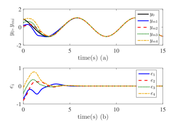
Figure 3: Control performance when PETM-C is not invoked. (a) Measurement outputs of leader and 4 followers; (b) Output regulation errors of 4 followers.

The PET distributed observer and output feedback controller are respectively given by (8)-(11) and (15)-(20) with $\mu_{1}=\mu_{2}=3$, $\iota_{S}=\iota_{v}=2$, $\gamma_{S}=\gamma_{v}=1$; $K_{i}=[-5\thinspace-5]$, $L_{i}=[-5\thinspace-5]$, $\sigma_{i}=\rho_{i}=1(i=1,2,3,4)$, $\kappa=30$, $\iota_{\psi}=2$, $\gamma_{\psi}=1$. Based on (14) and (22), the sampling period is selected as $T=\mathcal{T}^{i}=0.01s(i=1,2,3,4)$. The control performance of the multi-agent systems is shown in Fig. 3. It can be seen that the output of each follower quickly follows the output of the leader. Meanwhile, the regulation errors of the four followers all converge to zero. This indicates that cooperative output regulation has been achieved.

Fig. 4(a) and Fig. 4(b) show the event-triggered instants for the communication between each agent pair, and the sensor-to-controller transmission in each agent respectively. We observe many time intervals which do not have data communication. This implies that the communication burden has been reduced considerably. Fig. 5 shows the inter-event time for the communication from agent 2 to agent 3, and the sensor-to-controller transmission in agent 2. We can see that a minimum inter-event time has been guaranteed. Moreover, all the inter-event times are multiples of sampling period. These results highlight the advantages of the PET output regulation.

4.1.2 Discussions on the control parameters

We will give some discussions on how the control parameters will influence the control performance of the multi-agent systems.

Fig. 6 shows the control performance of the multi-agent systems for different $\mu_{1},\mu_{2}$. We can see that the convergence speed increases a lot when the values of $\mu_{1},\mu_{2}$ change from 1 to 2. However, the convergence rate for $\mu_{1}=\mu_{2}=3$ is slightly faster than that for $\mu_{1}=\mu_{2}=2$. This verifies Remark 7 and shows that when $\mu_{1},\mu_{2}$ are too large, the convergence speed does not increase considerably. Therefore, $\mu_{1},\mu_{2}$ are recommended to be set between 2 and 3 for the simulation to save energy.

Tables 1-2 respectively show the event-triggered times for different values of $\iota_{S},\iota_{v}\iota_{\psi}$ and $\gamma_{S},\gamma_{v}\gamma_{\psi}$ in PETM-A and PETM-B. It can be clearly seen that the communication load is reduced when increasing $\iota_{S},\iota_{v}\iota_{\psi}$ and decreasing $\gamma_{S},\gamma_{v}\gamma_{\psi}$. Fig. 7 demonstrates the control performance when $\iota_{S},\iota_{v}\iota_{\psi}$ and $\gamma_{S},\gamma_{v}\gamma_{\psi}$ take different values. We can see that a longer convergence time is needed for larger $\iota_{S},\iota_{v}\iota_{\psi}$ and smaller $\gamma_{S},\gamma_{v}\gamma_{\psi}$. This verifies Remark 9.

Let us see how the parameters $\sigma_{i}$ and $\rho_{i}$ in (17) influence the performance of the multi-agent systems. Fig. 8 shows the outputs of the four followers for different $\sigma_{i},\rho_{i}$. We can see that the proposed controller is robust to the variations of $\sigma_{i},\rho_{i}$. The control performance is almost the same for different $\sigma_{i},\rho_{i}$. This implies that the selection of $\sigma_{i},\rho_{i}$ can be very flexible. Table 3 demonstrates the event-triggered times for different $\sigma_{i},\rho_{i}$. We can see that as stated in Remark 9, the communication burden is reduced considerably when $\sigma_{i}=\rho_{i}=1$. This also shows the advantages of the control scheme in Fig. 1 such that the controller should send some information to PETM-B to further reduce the communication burden.

Finally, let us see how the selections of the sampling periods $T$ and $\mathcal{T}^{i}$ will influence the control performance. As stated in Section 3.2, the sampling periods can be selected independently and be different from one another. Fig. 9 shows the control performance of the multi-agent systems under different $T,\mathcal{T}^{i}$. We can see that the multi-agent systems are robust to the variations of $T,\mathcal{T}^{i}$.

4.2 PETM-A, PETM-B and PETM-C are invoked

We assume that PETM-C is invoked in Fig. 1. The PET distributed observer and output feedback controller are given by (8)-(11) and (23)-(25) with $\overline{\iota}_{\psi}=\overline{\iota}_{\omega}=0.001$, $\iota_{\omega}=2$, $\gamma_{\omega}=1$. The other control parameters are the same as before. The regulation errors and control efforts are shown in Figs. 11-10. It can be seen that the regulation error has converged to a small neighborhood around the origin. According to (92) in Appendix D, we know for $\forall i\in\{1,2,...,N\}$, $\varLambda_{i}\leq\underset{i\in\{1,2,...,N\}}{\max}\varphi_{i8}(\overline{\iota}_{\psi},\overline{\iota}_{\omega},\mathcal{T}^{i})\leq 0.43$ with $\varepsilon=0.01$, $\zeta_{1}=0.4$, $\zeta_{2}=1$, $\zeta_{3}=0.4$. This is accord with Fig. 10. Note that as stated in Remark 11 the estimation of $\varLambda$ by (92) is somewhat conservative. Nevertheless, it can provide guidelines for the selections of the control parameters.

Fig. 11 shows the control performance under different $\overline{\iota}_{\psi},\overline{\iota}_{\omega}$. We observe that the regulation errors all converge to a small neighborhood of the origin for all the cases. This verifies the robustness of the proposed method. Meanwhile, Table 4 shows the regulation errors and event-triggered times for PETM-B and PETM-C with different $\overline{\iota}_{\psi},\overline{\iota}_{\omega}$. We can see that larger $\overline{\iota}_{\psi},\overline{\iota}_{\omega}$ can result in larger regulation errors but small communication burden. This verifies Remark 11.

In addition, Fig. 12 demonstrates the control performance when $S=\overline{\iota}_{\psi}=\overline{\iota}_{\omega}=0$. In this case, $v$ is a constant signal. It can be seen that the regulation error converges to exact zero even though PETM-C is invoked. This also verifies Remark 11.

Figure 2: Communication graph.

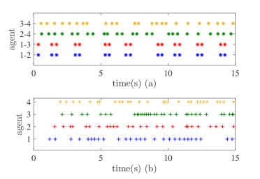
Figure 4: Event-triggered time instants. (a) Event-triggered time instants between each agent pair for PETM-A; (b) Event-triggered time instants of each agent for PETM-B.

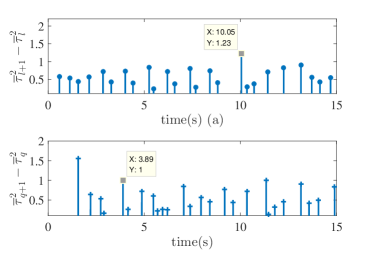
Figure 5: Inter-event time. (a) Inter-event time for the communication between agent 2 and 3; (b) Inter-event time between the sensor and controller in agent 2.

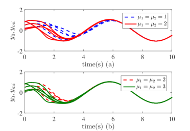
Figure 6: Control performance for different $\mu_{1},\mu_{2}$.

Table 1: Event-triggered times for PETM-A under different $\iota_{S},\iota_{v},\gamma_{S},\gamma_{v}$.

agent	1-2	1-3	2-4	3-4
$\iota_{S}=\iota_{v}=2,\gamma_{S}=\gamma_{v}=1$	18	18	26	25
$\iota_{S}=\iota_{v}=1,\gamma_{S}=\gamma_{v}=2$	30	30	37	37
$\iota_{S}=\iota_{v}=0.5,\gamma_{S}=\gamma_{v}=2.5$	79	79	120	94

Table 2: Event-triggered times for PETM-B under different $\iota_{\psi},\gamma_{\psi}$.

agent	1	2	3	4
$\iota_{\psi}=3,\gamma_{\psi}=0.5$	14	14	10	11
$\iota_{\psi}=2,\gamma_{\psi}=1$	27	26	20	24
$\iota_{\psi}=0.5,\gamma_{\psi}=1$	32	39	41	60

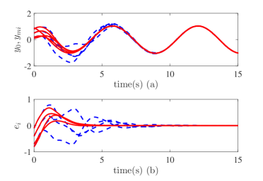
Figure 7: Control performance for different event-triggered conditions. (a) Measurement outputs of leader and 4 followers; (b) Output regulation errors of 4 followers. Blue dashed line: $\iota_{S}=\iota_{v}=2,\gamma_{S}=\gamma_{v}=1,\iota_{\psi}=3,\gamma_{\psi}=0.5$; red solid line: $\iota_{S}=\iota_{v}=0.5,\gamma_{S}=\gamma_{v}=2.5,\iota_{\psi}=0.5,\gamma_{\psi}=1$.

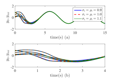
Figure 8: Control performance for different $\sigma_{i},\rho_{i}$.

Table 3: Event-triggered times for PETM-B under different $\sigma_{i},\rho_{i}$.

$\sigma_{i},\rho_{i}$	0	$0.8$	$0.9$	$1.0$	$1.1$	$1.2$
PETM-B	971	845	769	34	765	843

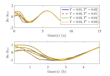
Figure 9: Control performance for different sampling periods $T,\mathcal{T}^{i}$. (a) Measurement outputs of leader and 4 followers; (b) Partial enlarged view of subfigure (a).

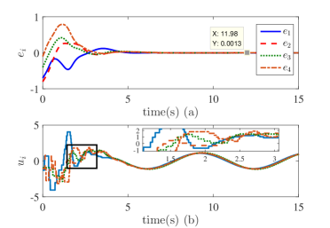
Figure 10: Control performance when PETM-C is invoked. (a) Output regulation errors of 4 followers; (b) Control efforts of 4 followers.

Figure 11: Control performance for different $\overline{\iota}_{\psi},\overline{\iota}_{\omega}$ when PETM-C is invoked. (a) Measurement outputs of leader and 4 followers; (b) Partial enlarged view of subfigure (a).

Table 4: Event-triggered times for PETM-B under different $\overline{\iota}_{\psi},\overline{\iota}_{\omega}$.

	error	PETM-B	PETM-C
$\overline{\iota}_{\psi}=\overline{\iota}_{\omega}=0$	0.0008	286	1015
$\overline{\iota}_{\psi}=\overline{\iota}_{\omega}=0.001$	0.0013	17	984
$\overline{\iota}_{\psi}=\overline{\iota}_{\omega}=0.01$	0.0070	13	597
$\overline{\iota}_{\psi}=\overline{\iota}_{\omega}=0.02$	0.0132	12	366

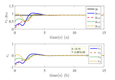
Figure 12: Control performance when PETM-C is invoked and $S=0,\overline{\iota}_{\psi}=\overline{\iota}_{\omega}=0$. (a) Measurement outputs of leader and 4 followers; (b) Output regulation errors of 4 followers.

5 Conclusions

In this paper, a new PET distributed observer and dynamic output feedback controller are proposed to solve the cooperative output regulation problem. PET mechanisms are simultaneously considered in the communication among different agents, sensor-to-controller and controller-to-actuator channels. Future works include considering fully distributed PET output regulation problem under asynchronous sampled data.

Appendix A Proof of Theorem 1

Proof.

In the following let $c_{i}(i=1,2,...,16)$ denote some proper positive constants. $\varepsilon$ represents an arbitrary small positive constant. The proof is then divided into the following steps.

Step 1. We will find the relation between $||\hat{S}_{i}(t)-\hat{S}_{i}(t_{k})||$ and $||\hat{S}_{i}(t)-S||(i=1,2,...,N)$.

Integrating (8) on time interval $[t_{k},t)\subseteq[t_{k},t_{k+1})$, we get

$$\hat{S}_{i}(t)-\hat{S}_{i}(t_{k})=(t-t_{k})\mu_{1}\sum_{j=0}^{N}a_{ij}(\hat{S}_{j}(\overline{t}_{l^{\prime}}^{j})-\hat{S}_{j}(\overline{t}_{l}^{i})).$$ (28)

It follows that

$$\hat{S}-\hat{S}(t_{k})= -\mu_{1}(t-t_{k})(\mathcal{H}\varotimes I)(\hat{S}(\overline{t}_{l})-\hat{S}(t_{k}))$$

$$-\mu_{1}(t-t_{k})(\mathcal{H}\varotimes I)(\hat{S}(t_{k})-\hat{S})$$

$$-\mu_{1}(t-t_{k})(\mathcal{H}\varotimes I)\tilde{S}$$ (29)

where $\hat{S}\triangleq\mathrm{col}(\hat{S}_{1},\hat{S}_{2},...,\hat{S}_{N})$, $\check{S}\triangleq\mathrm{col}(S,S,...,S)$, $\tilde{S}\triangleq\hat{S}-\check{S}$, $\hat{S}(\overline{t}_{l})\triangleq\mathrm{col}(\hat{S}_{1}(\overline{t}_{l^{\prime}}^{1}),\hat{S}_{2}(\overline{t}_{l^{\prime}}^{2}),...,\hat{S}_{N}(\overline{t}_{l^{\prime}}^{N}))$.

Next, we transform (29) into a vector form. Denote $\tilde{S}=[\tilde{s}_{1}\thinspace\tilde{s}_{2}\thinspace...\thinspace\tilde{s}_{n_{v}}]$, $\hat{S}(t_{k})-\hat{S}=[\Delta\hat{s}_{1}(t_{k})\thinspace\Delta\hat{s}_{2}(t_{k})\thinspace...\thinspace\Delta\hat{s}_{n_{v}}(t_{k})]$ and $\hat{S}(\overline{t}_{l})-\hat{S}(t_{k})=[\Delta\hat{s}_{1}(\overline{t}_{l})\thinspace\Delta\hat{s}_{2}(\overline{t}_{l})\thinspace...\thinspace\Delta\hat{s}_{n_{v}}(\overline{t}_{l})]$ where $\tilde{s}_{m},\Delta\hat{s}_{m}(t_{k}),\Delta\hat{s}_{m}(\overline{t}_{l})(m=1,2,...,n_{v})\in\mathbb{R}^{n_{v}N\times 1}$ are all column vectors. Then we have

$$\Delta\hat{s}_{m}(t_{k}) =-\mu_{1}(t-t_{k})(\mathcal{H}\varotimes I)(\Delta\hat{s}_{m}(\overline{t}_{l})+\Delta\hat{s}_{m}(t_{k})-\tilde{s}_{m}).$$

It follows that

$$||\Delta\hat{s}_{m}(t_{k})|| \leq\delta_{1}(T)(||\Delta\hat{s}_{m}(\overline{t}_{l})||+||\Delta\hat{s}_{m}(t_{k})||+||\tilde{s}_{m}||)$$

where $\delta_{1}(T)$ is a $\mathcal{K}$-class function such that

$$\delta_{1}(T)=\mu_{1}T||\mathcal{H}\varotimes I||.$$ (30)

Therefore, there exists a small enough $T$ such that $\delta_{1}(T)<1$. Then we obtain

$$||\Delta\hat{s}_{m}(t_{k})|| \leq\delta_{S}(T)||\tilde{s}_{m}||+\delta_{S}(T)||\Delta\hat{s}_{m}(\overline{t}_{l})||$$

where

$$\delta_{S}(T)=\frac{\delta_{1}(T)}{1-\delta_{1}(T)}.$$ (31)

Finally, according to the event-triggered condition (11), we know

$$||\Delta\hat{s}_{m}(t_{k})|| \leq\delta_{S}(T)||\tilde{s}_{m}||+c_{1}\mathrm{e}^{-\gamma_{S}t_{k}}.$$ (32)

Step 2. We will show $\tilde{S}_{i}$ converges to zero exponentially.

Note that (8) can be transformed into

$$\dot{\tilde{s}}_{m} =-\mu_{1}(\mathcal{H}\varotimes I)(\tilde{s}_{m}+\Delta\hat{s}_{m}(\overline{t}_{l})+\Delta\hat{s}_{m}(t_{k}))$$

for $m=1,2,...,n_{v}$.

Take the following Lyapunov function

$$V_{m}=\frac{1}{2}\tilde{s}_{m}^{T}(P\varotimes I)\tilde{s}_{m}$$

where $P$ is a positive matrix such that $P\mathcal{H}+\mathcal{H}^{T}P=2I$. Note that $P$ exists due to $-\mathcal{H}$ is Hurwitz from Lemma 1.

Then, we get

$$\dot{V}_{m}= -\mu_{1}||\tilde{s}_{m}||^{2}-\mu_{1}\tilde{s}_{m}^{T}(P\mathcal{H}\varotimes I)(\Delta\hat{s}_{m}(\overline{t}_{l})+\Delta\hat{s}_{m}(t_{k})).$$

Using Young’s inequality and (11), (32), we obtain

$$\dot{V}_{m}\leq -\left(\mu_{1}-\mu_{1}||P\mathcal{H}\varotimes I||\delta_{S}(T)-\varepsilon\right)||\tilde{s}_{m}||^{2}$$

$$+c_{2}\mathrm{e}^{-2\gamma_{S}t_{k}}.$$ (33)

Therefore, when $\delta_{S}(T)$ satisfies

$$\delta_{S}(T)<\frac{1}{||P\mathcal{H}\varotimes I||},$$ (34)

we have $\mu_{1}-\mu_{1}||P\mathcal{H}\varotimes I||\delta_{S}(T)-\varepsilon>0$. Then solving equation (33), we can obtain that $V_{m},\tilde{s}_{m},\tilde{S}$ will all converge to zero exponentially.

Combining (30), (31) and (34), note $||P\mathcal{H}\varotimes I||=||P\mathcal{H}||$, $||\mathcal{H}\varotimes I||=||\mathcal{H}||$, we know $T$ should satisfy

$$T<\frac{1}{\mu_{1}\left(||P\mathcal{H}||+1\right)||\mathcal{H}||}.$$ (35)

Step 3. We will show $\hat{v}$ does not exhibit finite time escape, $i.e.$, $\hat{v}$ is bounded on a finite time interval $[0,t)$.

Let $\overline{v}_{i}^{*}(t,t_{k},\overline{t}_{l}^{i})=\mathrm{e}^{\hat{S}_{i}(\overline{t}_{l}^{i})(t-t_{k})}\hat{v}_{i}(t_{k})(i=1,2,...,N)$, then (9) can be written as:

$$\dot{\hat{v}}_{i}= \hat{S}_{i}(\overline{t}_{l}^{i})\hat{v}_{i}(t)+\mu_{2}\sum_{j=0}^{N}a_{ij}(\overline{v}_{j}^{*}(t,t_{k},\overline{t}_{l^{\prime}}^{j})-\overline{v}_{i}^{*}(t,t_{k},\overline{t}_{l}^{i}))$$

$$+\mu_{2}\sum_{j=0}^{N}a_{ij}(\Delta\upsilon_{j}(t,t_{k},\overline{t}_{l^{\prime}}^{j})-\Delta\upsilon_{i}(t,t_{k},\overline{t}_{l}^{i}))$$ (36)

where $\Delta\upsilon_{i}(t,t_{k},\overline{t}_{l}^{i})=\overline{v}_{i}(t,\overline{t}_{l}^{i})-\overline{v}_{i}^{*}(t,t_{k},\overline{t}_{l}^{i}).$

Solving (36) on time interval $[t_{k},t_{k+1})$, we have

$$\hat{v}_{i}(t)= \overline{v}_{i}^{*}(t,t_{k},\overline{t}_{l}^{i})-\mu_{2}(t-t_{k})\sum_{j=0}^{N}a_{ij}\overline{v}_{i}^{*}(t,t_{k},\overline{t}_{l}^{i})$$

$$+\sum_{j=0}^{N}\mu_{2}\int_{t_{k}}^{t}a_{ij}\mathrm{e}^{-\hat{S}_{i}(\overline{t}_{l}^{i})(\tau-t)}\overline{v}_{j}^{*}(\tau,t_{k},\overline{t}_{l^{\prime}}^{j})d\tau$$ (37)

$$+\Delta\overline{\upsilon}_{i}$$

where

$$\Delta\overline{\upsilon}_{i}= \int_{t_{k}}^{t}\mathrm{e}^{-\hat{S}_{i}(\overline{t}_{l}^{i})(\tau-t)}\left(\mu_{2}\sum_{j=0}^{N}a_{ij}(\Delta\upsilon_{j}(\tau)-\Delta\upsilon_{i}(\tau))\right)d\tau.$$

For the terms in (37), we have

$$\mu_{2}\int_{t_{k}}^{t}a_{ij}\mathrm{e}^{-\hat{S}_{i}(\overline{t}_{l}^{i})(\tau-t)}\overline{v}_{j}^{*}(\tau,t_{k},\overline{t}_{l^{\prime}}^{j})d\tau$$

$$= \mu_{2}(t-t_{k})a_{ij}\overline{v}_{j}^{*}(t,t_{k},\overline{t}_{l^{\prime}}^{j})+\mu_{2}a_{ij}E_{ij}(t)\overline{v}_{j}^{*}(t,t_{k},\overline{t}_{l^{\prime}}^{j})$$ (38)

where $E_{ij}(t)$ is a time-varying matrix such that

$$E_{ij}(t)\triangleq\int_{t_{k}}^{t}(\mathrm{e}^{-\hat{S}_{i}(\overline{t}_{l}^{i})(\tau-t)}-\mathrm{e}^{-\hat{S}_{j}(\overline{t}_{l^{\prime}}^{j})(\tau-t)})\mathrm{e}^{\hat{S}_{j}(\overline{t}_{l^{\prime}}^{j})(\tau-t)}d\tau.$$ (39)

Substituting (38) into (37), we have

$$\hat{v}_{i}(t)= \overline{v}_{i}^{*}(t,t_{k},\overline{t}_{l}^{i})$$

$$+\mu_{2}(t-t_{k})\sum_{j=0}^{N}a_{ij}(\overline{v}_{j}^{*}(t,t_{k},\overline{t}_{l^{\prime}}^{j})-\overline{v}_{i}^{*}(t,t_{k},\overline{t}_{l}^{i}))$$

$$+\mu_{2}\sum_{j=0}^{N}a_{ij}E_{ij}(t)\overline{v}_{j}^{*}(t,t_{k},\overline{t}_{l^{\prime}}^{j})$$

$$+\Delta\overline{\upsilon}_{i}.$$

For $i=1,2,...,N$, we have

$$\hat{v}-\overline{v}^{*}(t,t_{k},\overline{t}_{l})$$

$$= \mu_{2}(t-t_{k})(\mathcal{H}\varotimes I)(\overline{v}^{*}(t,t_{k},\overline{t}_{l})-\check{v})+\mu_{2}\epsilon+\Delta\overline{\upsilon}$$ (40)

where $\hat{v}\triangleq\mathrm{col}(\hat{v}_{1},\hat{v}_{2},...,\hat{v}_{N})$, $\check{v}\triangleq\mathrm{col}(v,v,...,v)$,

$$\overline{v}^{*}(t,t_{k},\overline{t}_{l})\triangleq\mathrm{col}(\overline{v}_{1}^{*}(t,t_{k},\overline{t}_{l^{\prime}}^{1}),\overline{v}_{2}^{*}(t,t_{k},\overline{t}_{l^{\prime}}^{2}),...,\overline{v}_{N}^{*}(t,t_{k},\overline{t}_{l^{\prime}}^{N})),$$

$$\epsilon\triangleq\mathrm{col}\left(\epsilon_{1},\epsilon_{2}...,\epsilon_{N}\right),$$

$$\Delta\overline{\upsilon}\triangleq\mathrm{col}\left(\Delta\overline{\upsilon}_{1},\Delta\overline{\upsilon}_{2},...,\Delta\overline{\upsilon}_{N}\right)$$

with $\epsilon_{i}=\sum_{j=0}^{N}a_{ij}E_{ij}(t)\overline{v}_{j}^{*}(t,t_{k},\overline{t}_{l^{\prime}}^{j})(i=1,2,...,N)$.

Note that for the elements in $\epsilon$ and using Lemma 3,

$$||a_{ij}E_{ij}(t)\overline{v}_{j}^{*}(t,t_{k},\overline{t}_{l^{\prime}}^{j})||\leq a_{ij}||\overline{v}_{j}^{*}||\cdot||E_{ij}(t)||.$$ (41)

From (39) and Appendix B, we know $||E_{ij}(t)||$ converges to zero exponentially. Hence, using (41) for $\epsilon$, there exist positive constants $c_{3},c_{4}$ such that

$$||\epsilon||\leq c_{3}\mathrm{e}^{-c_{4}t}||\overline{v}^{*}(t,t_{k},\overline{t}_{l})||.$$ (42)

Meanwhile, according to Appendix B, we know there exist positive constants $c_{5},c_{6}$ such that

$$||\Delta\overline{\upsilon}||\leq c_{5}\mathrm{e}^{-c_{6}t}.$$ (43)

Then using (42) and (43) for (40), we obtain:

$$||\hat{v}-\overline{v}^{*}(t,t_{k},\overline{t}_{l})||\leq (\delta_{2}(T)+\mu_{2}c_{3}\mathrm{e}^{-c_{4}t})||\overline{v}^{*}(t,t_{k},\overline{t}_{l})||$$

$$+\delta_{2}(T)||\check{v}||+c_{5}\mathrm{e}^{-c_{6}t}$$ (44)

where $\delta_{2}(T)$ is a $\mathcal{K}$-class function such that

$$\delta_{2}(T)=\mu_{2}T||\mathcal{H}\varotimes I||.$$ (45)

It follows that

$$||\hat{v}|| \leq c_{7}||\overline{v}^{*}(t,t_{k},\overline{t}_{l})||+c_{8}\mathrm{e}^{-c_{9}t}+c_{10}$$

$$\mathrm{\leq\mathit{c}_{7}e}^{||\hat{S}_{i}(\overline{t}_{l}^{i})(t-t_{k})||}\hat{v}_{i}(t_{k})+c_{8}\mathrm{e}^{-c_{9}t}+c_{10}$$

It can be seen that $\hat{v}$ will not exhibit finite time escape.

Step 4. We will find the relation between $||\hat{v}-\overline{v}^{*}(t,t_{k},\overline{t}_{l})||$ and $||\tilde{v}||\triangleq||\hat{v}-\check{v}||$. Note that (40) can be expressed as:

$$\hat{v}-\overline{v}^{*}(t,t_{k},\overline{t}_{l})= \mu_{2}(t-t_{k})(\mathcal{H}\varotimes I)(\overline{v}^{*}(t,t_{k},\overline{t}_{l})-\hat{v})$$

$$+\mu_{2}(t-t_{k})(\mathcal{H}\varotimes I)\tilde{v}+\mu_{2}\epsilon+\Delta\overline{\upsilon}$$

where $\tilde{v}\triangleq\hat{v}-\check{v}$.

Using (42) and (43), we have

$$||\hat{v}-\overline{v}^{*}(t,t_{k},\overline{t}_{l})||$$

$$\leq (\delta_{2}(T)+\mu_{2}c_{3}\mathrm{e}^{-\mu_{1}c_{4}t})||\overline{v}^{*}(t,t_{k},\overline{t}_{l})-\hat{v}||$$

$$+(\delta_{2}(T)+\mu_{2}c_{3}\mathrm{e}^{-c_{4}t})||\tilde{v}||$$

$$+\mu_{2}c_{3}\mathrm{e}^{-c_{4}t}||\check{v}||+c_{5}\mathrm{e}^{-c_{6}t}.$$ (46)

Next, define a set $\Omega_{L}$ for the sampling instant $t_{k}$ which will be used in the following analysis.

By (44), we know if $T$ is small enough, $\delta_{2}(T)<1$ is true. Thus, it can be concluded that there exists a finite integer $k_{1}$ such that for $\forall t\in[t_{k},t_{k+1})$ with $k\geq k_{1}$, we have $\delta_{2}(T)+\mu_{2}c_{3}\mathrm{e}^{-c_{4}t}<1$ and $\mu_{2}c_{3}\mathrm{e}^{-c_{4}t}<\varepsilon$ where $\varepsilon$ can be an arbitrary small constant.

Also note that according to Step 2, we know $\hat{S}$ converges to $S$ exponentially. Therefore, there exist positive constants $c_{11},c_{12}$ such that $||S_{d}||\leq c_{11}\mathrm{e}^{-c_{12}t}$ where $S_{d}(\overline{t}_{l})=\mathrm{diag}(\hat{S}_{1}(\overline{t}_{l^{\prime}}^{1})-S,\hat{S}_{1}(\overline{t}_{l^{\prime}}^{2})-S,...,\hat{S}_{N}(\overline{t}_{l^{\prime}}^{N})-S)$. This means that there exists a finite integer $k_{2}$ such that for $\forall t\in[t_{k},t_{k+1})$ with $k\geq k_{2}$, we have $||S_{d}||\leq c_{11}\mathrm{e}^{-c_{12}t}<\varepsilon$ where $\varepsilon$ is an arbitrary small constant.

Then define the set $\Omega_{L}$ as

$$\Omega_{L}\triangleq\{t_{k}|k\in\mathbb{N},k\geq\mathrm{max}(k_{1},k_{2})\}.$$

Therefore, for $\forall t\in[t_{k},t_{k+1})$ with $t_{k},t_{k+1}\in\Omega_{L}$, (46) can be written as:

$$||\hat{v}-\overline{v}^{*}(t,t_{k},\overline{t}_{l})||\leq\delta_{v}(T)||\tilde{v}||+c_{13}\mathrm{e}^{-c_{14}t}$$ (47)

where

$$\delta_{v}(T)=\frac{(\delta_{2}(T)+\mu_{2}c_{3}\mathrm{e}^{-\mu_{1}c_{4}t})}{1-(\delta_{2}(T)+\mu_{2}c_{3}\mathrm{e}^{-\mu_{1}c_{4}t})}.$$ (48)

Step 5. We will show $\tilde{v}_{i}$ converges to zero exponentially.

We consider our analysis for $t\in[t_{k},t_{k+1})$ with $t_{k},t_{k+1}\in\Omega_{L}$. Note that from Step 3), we know $\hat{v}_{i}$ will not exhibit finite time escape. Hence, for any finite $k$, $\hat{v}_{i}$ is bounded on $[t_{k},t_{k+1})$ .

By (9), we have

$$\dot{\tilde{v}}= (I\varotimes S-\mu_{2}\mathcal{H}\varotimes I)\tilde{v}+S_{d}\tilde{v}+S_{d}\check{v}$$

$$-\mu_{2}(\mathcal{H}\varotimes I)(\overline{v}^{*}(t,t_{k},\overline{t}_{l})-\hat{v}).$$ (49)

Take the following Lyapunov function

$$V_{v}=\frac{1}{2}\tilde{v}^{T}(P\varotimes I)\tilde{v}$$

where $P$ is a positive matrix such that $P\mathcal{H}+\mathcal{H}^{T}P=2I$.

The derivative of $V_{v}$ is computed as:

$$\dot{V}_{v}= \tilde{v}^{T}(P\varotimes I)(I\varotimes S-\mu_{2}\mathcal{H}\varotimes I)\tilde{v}$$

$$+\tilde{v}^{T}(P\varotimes I)S_{d}\tilde{v}+\tilde{v}^{T}(D\varotimes I)S_{d}\check{v}$$

$$-\tilde{v}^{T}(P\varotimes I)\mu_{2}(\mathcal{H}\varotimes I)(\overline{v}^{*}(t,t_{k},\overline{t}_{l})-\hat{v}).$$

Using (47), we have

$$\dot{V}_{v}\leq \tilde{v}^{T}(P\varotimes S)\tilde{v}-\mu_{2}\lambda||\tilde{v}||^{2}$$

$$+||\tilde{v}||^{2}||P\varotimes I||\cdot||S_{d}||+||\tilde{v}||\cdot||(P\varotimes I)S_{d}\check{v}||$$

$$+\mu_{2}||P\mathcal{H}\varotimes I||\cdot||\tilde{v}||\left(\delta_{v}(T)||\tilde{v}||+c_{13}\mathrm{e}^{-c_{14}t}\right).$$

Note that due to $S$ is a skew-symmetric matrix, $(P\varotimes S)^{\rm T}=P\varotimes S^{\rm T}=-(P\varotimes S)$. This means that $P\varotimes S$ is also a skew-symmetric matrix. Hence, $\tilde{v}^{\rm T}(P\varotimes S)\tilde{v}=0$. Also note that $||S_{d}||\leq c_{11}\mathrm{e}^{-c_{12}t}<\varepsilon$ for $t\in[t_{k},t_{k+1})$ with $t_{k},t_{k+1}\in\Omega_{L}$. Thus, by Young’s inequality, we obtain:

$$\dot{V}_{v}\leq -\left(\mu_{2}-||P\varotimes I||\varepsilon-\mu_{2}||P\mathcal{H}\varotimes I||\delta_{v}(T)-\varepsilon\right)||\tilde{v}||^{2}$$

$$+c_{15}\mathrm{e}^{-2c_{12}t}+c_{16}\mathrm{e}^{-2c_{14}t}.$$

Hence, when

$$\delta_{v}(T)<\mu_{2}$$ (50)

we can obtain $\mu_{2}-||D\varotimes I||\varepsilon-\mu_{2}||D\mathcal{H}\varotimes I||\delta_{v}(T)-\varepsilon<0$. Then by solving the above equation, we can show $V_{v},\tilde{v}$ converge to zero exponentially. The proof is completed.

For the selection of $T$. Based on (45), (48), (50), (35) and note $\mu_{2}c_{3}\mathrm{e}^{-c_{4}t}<\varepsilon$, $c_{11}\mathrm{e}^{-c_{12}t}<\varepsilon$, we know $T$ should satisfy (14). ∎

Appendix B Proposition 1

Proposition 1.

$||E_{ij}(t)||_{F}$ in (39) and $||\Delta\overline{\upsilon}||$ in (40) both converge to zero exponentially.

Proof.

We first show $||E_{ij}(t)||_{F}$ converge to zero exponentially. Note that from Steps 1-2 in Appendix A, we know $\tilde{S}_{i}$ converges to zero exponentially for $\forall i=1,2,...,N$. Hence, $\hat{S}_{i}(t_{k}),\hat{S}_{j}(t_{k})$ are both bounded. Then by Lemma 3, we have

$$||E_{ij}(t)||$$

$$\leq \int_{t_{k}}^{t}||(\mathrm{e}^{-\hat{S}_{j}(t_{k})(\tau-t)}-\mathrm{e}^{-\hat{S}_{i}(t_{k})(\tau-t)})||\cdot||\mathrm{e}^{\hat{S}_{j}(t_{k})(\tau-t_{k})}||d\tau$$

$$\leq g_{1}\int_{t_{k}}^{t}||X(t_{k})(\tau-t)||\mathrm{e}^{||X(t_{k})(\tau-t)||+||Y(t_{k})(\tau-t)||}d\tau$$

where $X(t)=\hat{S}_{j}(t)-\hat{S}_{i}(t)$, $Y(t)=\hat{S}_{i}(t)$, $g_{1}>0$ is a positive constant.

Meanwhile, due to $||\tilde{S}||$ converge to zero exponentially, there exist constants $g_{2},g_{3}$ such that $||X||\leq g_{2}\mathrm{e}^{-g_{3}t}$. Hence, we have $||E_{ij}(t)||\leq g_{4}\mathrm{e}^{-g_{5}t}$where $g_{4},g_{5}>0$ are positive constants.

Next, we shall show $||\Delta\overline{\upsilon}||$ converge to zero exponentially. Recalling (11) and the definitions of $\overline{v}_{i}(t,\overline{t}_{l}^{i})$, $\overline{v}_{i}^{*}(t,t_{k},\overline{t}_{l}^{i})$, we have

$$||\Delta\upsilon_{i}(t,t_{k},\overline{t}_{l}^{i})|| =||\overline{v}_{i}(t,\overline{t}_{l}^{i})-\overline{v}_{i}^{*}(t,t_{k},\overline{t}_{l}^{i})||$$

$$=||\mathrm{e}^{\hat{S}_{i}(\overline{t}_{l}^{i})(t-\overline{t}_{l}^{i})}\hat{v}_{i}(\overline{t}_{l}^{i})-\mathrm{e}^{\hat{S}_{i}(\overline{t}_{l}^{i})(t-t_{k})}\hat{v}_{i}(t_{k})||$$

$$\leq||\mathrm{e}^{\hat{S}_{i}(\overline{t}_{l}^{i})(t-t_{k})}||\cdot||\mathrm{e}^{\hat{S}_{i}(\overline{t}_{l}^{i})(t_{k}-\overline{t}_{l}^{i})}-\hat{v}_{i}(t_{k})||$$

$$\leq g_{6}\mathrm{e}^{-g_{7}t}$$ (51)

where $g_{6},g_{7}>0$ are positive constants. Using the above equation for each element in $||\Delta\overline{\upsilon}||,$ the proof is completed. ∎

Appendix C Proof of Theorem 2

Proof.

The proof is divided into the following steps.

Step 1). We will find the relation between $\tilde{x}_{i}(t)$ and $\tilde{x}_{i}(\tau_{p}^{i})$ where $\tilde{x}_{i}\triangleq\hat{x}_{i}-x_{i}$.

Subtracting (3) from (17), we have

$$\dot{\tilde{x}}_{i}= A_{i}\tilde{x}_{i}+E_{i}\tilde{v}_{i}$$

$$+L_{i}(C_{mi}\hat{x}_{i}(\tau_{p}^{i})+D_{mi}u_{i}(\tau_{p}^{i}))$$

$$+L_{i}(\rho_{i}F_{i}\overline{v}_{i}(t,\overline{t}_{l}^{i})+(1-\sigma_{i})F_{mi}\overline{v}_{i}(t,\overline{t}_{l}^{i})+\psi_{i}(\tau_{p}^{i}))$$

$$+L_{i}(\psi_{i}(\overline{\tau}_{q}^{i})-\psi_{i}(\tau_{p}^{i})).$$ (52)

Then using (18) for $\psi_{i}(\tau_{p}^{i})$, we obtain

$$\dot{\tilde{x}}_{i}= A_{i}\tilde{x}_{i}+E_{i}\tilde{v}_{i}+L_{i}(C_{mi}\hat{x}_{i}(\tau_{p}^{i})+D_{mi}u_{i}(\tau_{p}^{i}))$$

$$+L_{i}(F_{mi}\overline{v}_{i}(\tau_{p}^{i},\overline{t}_{l}^{i})-y_{m}(\tau_{p}^{i}))$$

$$+L_{i}(\psi_{i}(\overline{\tau}_{q}^{i})-\psi_{i}(\tau_{p}^{i})).$$ (53)

Adopting (3) for $y_{m}(\tau_{p}^{i})$, we have

$$\dot{\tilde{x}}_{i}= (A_{i}+L_{i}C_{mi})\tilde{x}_{i}+L_{i}C_{mi}\left(\tilde{x}_{i}(\tau_{p}^{i})-\tilde{x}_{i}\right)$$

$$+E_{i}\tilde{v}_{i}+L_{i}F_{mi}\left(\overline{v}_{i}(\tau_{p}^{i},\overline{t}_{l}^{i})-v(\tau_{p}^{i})\right)$$

$$+L_{i}\left(\psi_{i}(\overline{\tau}_{q}^{i})-\psi_{i}(\tau_{p}^{i})\right).$$ (54)

Note that

$$\overline{v}_{i}(\tau_{p}^{i},\overline{t}_{l}^{i})-v(\tau_{p}^{i})= (\overline{v}_{i}(\tau_{p}^{i},\overline{t}_{l}^{i})-\hat{v}_{i}(\tau_{p}^{i})+\hat{v}_{i}(\tau_{p}^{i})-v(\tau_{p}^{i})).$$

From Theorem 1, we know $\overline{v}_{i}(\tau_{p}^{i},\overline{t}_{l}^{i})-\hat{v}_{i}(\tau_{p}^{i})$ and $\hat{v}_{i}(\tau_{p}^{i})-v(\tau_{p}^{i})$ will both converge to zero exponentially. Hence, $\overline{v}_{i}(\tau_{p}^{i},\overline{t}_{l}^{i})-v(\tau_{p}^{i})$ will converge to zero exponentially. Meanwhile, from Theorem 1 and (20) we know $\tilde{v}_{i}$ and $\psi_{i}(\overline{\tau}_{q}^{i})-\psi_{i}(\tau_{p}^{i})$ will also converge to zero exponentially. Hence, we can conclude that there exist positive constants $\mathrm{c}_{1},\mathrm{c}_{2}$ such that

$$||E_{i}\tilde{v}_{i}+L_{i}F_{mi}\left(\overline{v}_{i}(\tau_{p}^{i},\overline{t}_{l}^{i})-v(\tau_{p}^{i})\right)$$

$$+L_{i}\left(\psi_{i}(\overline{\tau}_{q}^{i})-\psi_{i}(\tau_{p}^{i})\right)|| <\mathrm{c}_{1}\mathrm{e}^{-\mathrm{c}_{2}t}.$$ (55)

Hence, integrating (54) on $[\tau_{p}^{i},\tau_{p+1}^{i})$ we get

$$\tilde{x}_{i}(t)-\tilde{x}_{i}(\tau_{p}^{i})= \int_{\tau_{p}^{i}}^{t}A_{i}\left(\tilde{x}_{i}(\tau)-\tilde{x}_{i}(\tau_{p}^{i})\right)d\tau$$

$$+(t-\tau_{p}^{i})(A_{i}+L_{i}C_{mi})\tilde{x}_{i}(\tau_{p}^{i})$$

$$+\int_{\tau_{p}^{i}}^{t}\mathrm{c}_{1}\mathrm{e}^{-\mathrm{c}_{2}\tau}d\tau.$$ (56)

It follows that

$$||\tilde{x}_{i}(t)-\tilde{x}_{i}(\tau_{p}^{i})||\leq \int_{\tau_{p}^{i}}^{t}||A_{i}||\cdot||\tilde{x}_{i}(\tau)-\tilde{x}_{i}(\tau_{p}^{i})||d\tau$$

$$+\mathcal{T}^{i}||A_{i}+L_{i}C_{mi}||\cdot||\tilde{x}_{i}(\tau_{p}^{i})||$$

$$+\mathcal{T}^{i}\mathrm{c}_{1}\mathrm{e}^{-\mathrm{c}_{2}\tau_{p}^{i}}.$$ (57)

By Gronwall’s inequality, we obtain

$$||\tilde{x}_{i}(t)-\tilde{x}_{i}(\tau_{p}^{i})||\leq \delta_{i3}(\mathcal{T}^{i})||\tilde{x}_{i}(\tau_{p}^{i})||$$

$$+\mathcal{T}^{i}\mathrm{e}^{||A_{i}||\mathcal{T}^{i}}\mathrm{c}_{1}\mathrm{e}^{-\mathrm{c}_{2}\tau_{p}^{i}}$$ (58)

where $\delta_{i3}(\mathcal{T}^{i})$ is a $\mathcal{K}$-class function such that

$$\delta_{i3}(\mathcal{T}^{i})=\mathcal{T}^{i}||A_{i}+L_{i}C_{mi}||\mathrm{e}^{||A_{i}||\mathcal{T}^{i}}.$$

When $\mathcal{T}^{i}$ is small enough such that $\delta_{i3}(\mathcal{T}^{i})<1$, then we have

$$||\tilde{x}_{i}-\tilde{x}_{i}(\tau_{p}^{i})|| \leq\delta_{\tilde{x}}(\mathcal{T}^{i})||\tilde{x}_{i}||+\mathrm{c}_{3}\mathrm{e}^{-\mathrm{c}_{2}t}$$ (59)

where $\mathrm{c}_{3}>0$ is a constant,

$$\delta_{\tilde{x}}(\mathcal{T}^{i})=\frac{\delta_{i3}(\mathcal{T}^{i})}{1-\delta_{i3}(\mathcal{T}^{i})}.$$ (60)

Step 2). We will show $\tilde{x}_{i},e_{i}$ converge to zero exponentially.

First, we demonstrate $\tilde{x}_{i}$ converge to zero exponentially. Note that $A_{i}+L_{i}C_{mi}$ is a Hurwitz matrix, then there exists a positive matrix $Q_{i}$ such that $Q_{i}(A_{i}+L_{i}C_{mi})+(A_{i}+L_{i}C_{mi})^{\mathrm{\mathit{T}}}Q_{i}=-2I$. Then consider the following Lyapunov function

$$V_{\tilde{x}}=\frac{1}{2}\tilde{x}_{i}^{T}Q_{i}\tilde{x}_{i}.$$

From (54), the derivative of $V_{\tilde{x}}$ is given by:

$$\dot{V}_{\tilde{x}}= -||\tilde{x}_{i}||^{2}+\tilde{x}_{i}^{T}Q_{i}L_{i}C_{mi}\left(\tilde{x}_{i}(\tau_{p}^{i})-\tilde{x}_{i}\right)$$

$$+\tilde{x}_{i}^{T}Q_{i}\left(E_{i}\tilde{v}_{i}+L_{i}F_{mi}\left(\overline{v}_{i}(\tau_{p}^{i},\overline{t}_{l}^{i})-v(\tau_{p}^{i})\right)\right)$$

$$+\tilde{x}_{i}^{T}Q_{i}L_{i}(\psi_{i}(\overline{\tau}_{q}^{i})-\psi_{i}(\tau_{p}^{i})).$$ (61)

Using (58) and (55), we get

$$\dot{V}_{\tilde{x}}\leq -(1-||Q_{i}L_{i}C_{mi}||\delta_{\tilde{x}}(\mathcal{T}^{i})-\varepsilon)||\tilde{x}_{i}||^{2}+\mathrm{c}_{4}\mathrm{e}^{-2\mathrm{c}_{2}t}$$

where $\varepsilon$ is an arbitrary small constant, $\mathrm{c}_{4}$ is a positive constant.

Therefore, when

$$||Q_{i}L_{i}C_{mi}||\delta_{\tilde{x}}(\mathcal{T}^{i})<1$$

then we can conclude that $\tilde{x}_{i}$ will converge to zero exponentially.

Next, we will prove $e_{i}$ converge to zero exponentially. Consider the following coordinate transformation $\overline{x}_{i}=x_{i}-X_{i}v$ and $\overline{u}_{i}=u_{i}-U_{i}v$. Then based on (5), (3) is expressed as:

$$\dot{\overline{x}}_{i}= A_{i}(\overline{x}_{i}+X_{i}v)+B_{i}(\overline{u}_{i}+U_{i}v)+E_{i}v-X_{i}Sv$$

$$= A\overline{x}_{i}+B\overline{u}_{i},$$ (62)

$$e_{i}= C_{i}(\overline{x}_{i}+X_{i}v)+D_{i}(\overline{u}_{i}+U_{i}v)+F_{i}v$$

$$= C_{i}\overline{x}_{i}+D_{i}\overline{u}_{i}.$$ (63)

By (15), $\overline{u}_{i}$ is expressed as:

$$\overline{u}_{i}= K_{i}\hat{x}_{i}+(\hat{U}_{i}-K_{i}\hat{X}_{i})\hat{v}_{i}-U_{i}v$$

$$= K_{i}\overline{x}_{i}+K_{i}\tilde{x}_{i}+(\tilde{U}_{i}-K_{i}\tilde{X}_{i})\hat{v}_{i}+(U_{i}-K_{i}X_{i})\tilde{v}_{i}.$$

Then (62) is written as:

$$\dot{\overline{x}}_{i}= (A_{i}+B_{i}K_{i})\overline{x}_{i}$$

$$+K_{i}\tilde{x}_{i}+(\tilde{U}_{i}-K_{i}\tilde{X}_{i})\hat{v}_{i}+(U_{i}-K_{i}X_{i})\tilde{v}_{i}.$$

Note that $\tilde{x}_{i},\tilde{v}_{i},\tilde{X}_{i},\tilde{U}_{i}$ all converge to zero exponentially, and $A_{i}+B_{i}K_{i}$ is a Hurwitz matrix. Thus, $\overline{x}_{i}$ will converge to zero exponentially. Then $e_{i}$ will converge to zero exponentially. The proof is completed. ∎

Appendix D Proof of Theorem 3

Proof.

In the following let $\mathrm{c}_{j}(j=1,2,...,18)$ denote some proper positive constants. $\mathrm{\varphi}_{ij}(\overline{\iota}_{\psi},\overline{\iota}_{\omega},\mathcal{T}^{i})(j=1,2,...,8)$ denote some non-negative increasing functions for agent $i$ with $\mathrm{\varphi}_{ij}(0,0,0)=0$. $\zeta_{1},\zeta_{2},\zeta_{3},\varepsilon$ are some positive design parameters. The proof is then divided into the following steps.

Step 1). We will find the relation between $\tilde{x}_{i}(t)$ and $\tilde{x}_{i}(\tau_{p}^{i})$.

Using (24) and Theorem 1, we can obtain that

$$||E_{i}\tilde{v}_{i}+L_{i}F_{mi}\left(\overline{v}_{i}(\tau_{p}^{i},\overline{t}_{l}^{i})-v(\tau_{p}^{i})\right)$$

$$+L_{i}\left(\psi_{i}(\overline{\tau}_{q}^{i})-\psi_{i}(\tau_{p}^{i})\right)|| <\mathrm{c}_{1}\mathrm{e}^{-\mathrm{c}_{2}t}+||L_{i}||\overline{\iota}_{\psi}.$$ (64)

Then by following the line of Step 1) in the proof of Theorem 2 and using the above inequality, we get

$$||\tilde{x}_{i}(t)-\tilde{x}_{i}(\tau_{p}^{i})||\leq \delta_{i3}(\mathcal{T}^{i})||\tilde{x}_{i}(\tau_{p}^{i})||+\mathcal{T}^{i}\mathrm{e}^{||A_{i}||\mathcal{T}^{i}}\mathrm{c}_{1}\mathrm{e}^{-\mathrm{c}_{2}\tau_{p}^{i}}$$

$$+\mathcal{T}^{i}||L_{i}||\overline{\iota}_{\psi}\mathrm{e}^{||A_{i}||\mathcal{T}^{i}}.$$ (65)

Then when $\mathcal{T}^{i}$ is small enough, we have

$$||\tilde{x}_{i}-\tilde{x}_{i}(\tau_{p}^{i})||\leq \delta_{\tilde{x}}(\mathcal{T}^{i})||\tilde{x}_{i}||+\mathrm{c}_{3}\mathrm{e}^{-\mathrm{c}_{2}t}+\mathrm{\varphi}_{i1}(\cdot)$$ (66)

where

$$\mathrm{\varphi}_{i1}(\overline{\iota}_{\psi},\overline{\iota}_{\omega},\mathcal{T}^{i})=\frac{\mathcal{T}^{i}||L_{i}||\overline{\iota}_{\psi}\mathrm{e}^{||A_{i}||\mathcal{T}^{i}}}{1-\delta_{i3}(\mathcal{T}^{i})}.$$ (67)

Step 2). We will show $\tilde{x}_{i}$ will converge to a small neighborhood of origin.

Consider the Lyapunov function $V_{\tilde{x}}=\frac{1}{2}\tilde{x}_{i}^{T}Q_{i}\tilde{x}_{i}.$ Based on (61), (66), (24) and Theorem 1, we obtain

$$\dot{V}_{\tilde{x}}\leq -||\tilde{x}_{i}||^{2}+||Q_{i}L_{i}C_{mi}||\delta_{\tilde{x}}(\mathcal{T}^{i})||\tilde{x}_{i}||^{2}$$

$$+||\tilde{x}_{i}||\cdot||Q_{i}L_{i}C_{mi}||\varphi_{i1}(\mathcal{T}^{i},\overline{\iota}_{\psi})+||\tilde{x}_{i}||\cdot||Q_{i}L_{i}||\overline{\iota}_{\psi}$$

$$+||\tilde{x}_{i}||\mathrm{c}_{4}\mathrm{e}^{-\mathrm{c}_{5}t}.$$

By Young’s inequality, we have

$$\dot{V}_{\tilde{x}}\leq -(1-||Q_{i}L_{i}C_{mi}||\delta_{\tilde{x}}(\mathcal{T}^{i})-\zeta_{1}-\varepsilon)||\tilde{x}_{i}||^{2}$$

$$+\mathrm{c}_{6}\mathrm{e}^{-2\mathrm{c}_{5}t}+\varphi_{i2}$$ (68)

where $\varepsilon>0$ is a small design parameter such that $||Q_{i}L_{i}C_{mi}||\delta_{\tilde{x}}(\mathcal{T}^{i})+\zeta_{1}+\varepsilon<1$,

$$\mathrm{\varphi}_{i2}(\overline{\iota}_{\psi},\overline{\iota}_{\omega},\mathcal{T}^{i})=\frac{\left(||Q_{i}L_{i}C_{mi}||\varphi_{i1}(\mathcal{T}^{i},\overline{\iota}_{\psi})+||Q_{i}L_{i}||\overline{\iota}_{\psi}\right)^{2}}{4\zeta_{1}}.$$ (69)

Note that

$$\frac{\lambda_{\min}(Q)||\tilde{x}_{i}||^{2}}{2}\leq V_{\tilde{x}}\leq\frac{\lambda_{\max}(Q)||\tilde{x}_{i}||^{2}}{2}.$$ (70)

Therefore, (68) can be expressed as:

$$\dot{V}_{\tilde{x}}\leq -(1-||Q_{i}L_{i}C_{mi}||\delta_{\tilde{x}}(\mathcal{T}^{i})-\zeta_{1}-\varepsilon)\frac{2V_{\tilde{x}}}{\lambda_{\max}(Q)}$$

$$+\mathrm{c}_{6}\mathrm{e}^{-2\mathrm{c}_{5}t}+\varphi_{i2}.$$ (71)

By solving the above inequality, we can conclude that

$$V_{\tilde{x}}\leq\mathrm{c}_{7}\mathrm{e}^{-\mathrm{c}_{8}t}+ \frac{\lambda_{\max}(Q)\varphi_{i2}}{2(1-||Q_{i}L_{i}C_{mi}||\delta_{\tilde{x}}(\mathcal{T}^{i})-\zeta_{1}-\varepsilon)}.$$ (72)

Using (70), we have

$$||\tilde{x}_{i}||\leq\frac{\mathrm{2c}_{7}\mathrm{e}^{-\mathrm{c}_{8}t}}{\lambda_{\min}(Q)}+\varphi_{i3}$$ (73)

where

$$\varphi_{i3}=\frac{\lambda_{\max}(Q)\varphi_{i2}}{\lambda_{\min}(Q)\left(1-||Q_{i}L_{i}C_{mi}||\delta_{\tilde{x}}(\mathcal{T}^{i})-\zeta_{1}-\varepsilon\right)}.$$ (74)

This shows that $\tilde{x}_{i}$ will converge to a small neighborhood of origin.

Step 3). We will find the relation between $\overline{x}_{i}$ and $\overline{x}_{i}(\tau_{p}^{i})$.

Using (23) and (16), $\overline{u}_{i}$ is expressed as:

$$\overline{u}_{i}= \omega_{i}(\tau_{p}^{i})+\omega_{i}(\overline{\varsigma}_{m}^{i})-\omega_{i}(\tau_{p}^{i})$$

$$= K_{i}\hat{x}_{i}(\tau_{p}^{i})+(\hat{U}_{i}(\tau_{p}^{i})-K_{i}\hat{X}_{i}(\tau_{p}^{i}))\hat{v}_{i}(\tau_{p}^{i})-U_{i}v$$

$$+\omega_{i}(\overline{\varsigma}_{m}^{i})-\omega_{i}(\tau_{p}^{i})$$

$$= K_{i}\overline{x}_{i}(\tau_{p}^{i})+\mathcal{U}_{i}$$ (75)

where

$$\mathcal{U}_{i}= K_{i}\tilde{x}_{i}(\tau_{p}^{i})+(\tilde{U}_{i}(\tau_{p}^{i})-K_{i}\tilde{X}_{i}(\tau_{p}^{i}))\hat{v}_{i}(\tau_{p}^{i})$$

$$+ (U_{i}-K_{i}X_{i})\tilde{v}_{i}(\tau_{p}^{i})+U_{i}(v(\tau_{p}^{i})-v(t))$$

$$+ (\omega_{i}(\overline{\varsigma}_{m}^{i})-\omega_{i}(\tau_{p}^{i})).$$

Substituting the above equation into (62), we obtain

$$\dot{\overline{x}}_{i}= A_{i}\overline{x}_{i}+B_{i}K_{i}\overline{x}_{i}(\tau_{p}^{i})+B_{i}\mathcal{U}_{i}$$ (76)

Note that there exists a non-negative constant $\zeta_{2}$ such that

$$||v(\tau_{p}^{i})-v(t)||\leq\zeta_{2}\mathcal{T}^{i}$$ (77)

where $\zeta_{2}=0$ when $v(t)$ is a constant signal.

Meanwhile, $\tilde{v}_{i},\tilde{X}_{i},\tilde{U}_{i}$ all converge to zero exponentially. Then by (73) and (25), we conclude that

$$||\mathcal{U}_{i}||\leq\mathrm{c}_{9}\mathrm{e}^{-\mathrm{c}_{10}t}+\varphi_{i4}(\overline{\iota}_{\psi},\overline{\iota}_{\omega},\mathcal{T}^{i})$$ (78)

where

$$\varphi_{i4}(\overline{\iota}_{\psi},\overline{\iota}_{\omega},\mathcal{T}^{i})=||K_{i}\varphi_{i3}||+\overline{\iota}_{\omega}+||U_{i}\zeta_{2}\mathcal{T}^{i}||.$$ (79)

Using this for (76) and by Gronwall’s inequality, we obtain

$$||\overline{x}_{i}-\overline{x}_{i}(\tau_{p}^{i})||\leq \delta_{i4}(\mathcal{T}^{i})||\overline{x}_{i}(\tau_{p}^{i})||+\mathcal{T}^{i}\mathrm{e}^{||A_{i}||\mathcal{T}^{i}}\mathrm{c}_{9}\mathrm{e}^{-\mathrm{c}_{10}\tau_{p}^{i}}$$

$$+\mathcal{T}^{i}\mathrm{e}^{||A_{i}||\mathcal{T}^{i}}\varphi_{i4}(\overline{\iota}_{\psi},\overline{\iota}_{\omega},\mathcal{T}^{i})$$ (80)

where

$$\delta_{i4}(\mathcal{T}^{i})=\mathcal{T}^{i}||A_{i}+B_{i}K_{i}||\mathrm{e}^{||A_{i}||\mathcal{T}^{i}}.$$ (81)

Then when $\mathcal{T}^{i}$ is small enough, we have

$$||\overline{x}_{i}-\overline{x}_{i}(\tau_{p}^{i})|| \leq\delta_{\overline{x}}(\mathcal{T}^{i})||\overline{x}_{i}||+\mathrm{c}_{11}\mathrm{e}^{-\mathrm{c}_{12}t}+\varphi_{i5}$$ (82)

where

$$\delta_{\overline{x}}(\mathcal{T}^{i})=\frac{\delta_{i4}(\mathcal{T}^{i})}{1-\delta_{i4}(\mathcal{T}^{i})},$$ (83)

$$\varphi_{i5}=\frac{\mathcal{T}^{i}\mathrm{e}^{||A_{i}||\mathcal{T}^{i}}\varphi_{i4}(\overline{\iota}_{\psi},\overline{\iota}_{\omega},\mathcal{T}^{i})}{1-\delta_{i4}(\mathcal{T}^{i})}.$$ (84)

Step 4). We will show $\overline{x}_{i},e_{i}$ converge to a small neighborhood of origin.

Consider

$$V_{\overline{x}}=\frac{1}{2}\overline{x}_{i}^{T}R_{i}\overline{x}_{i}$$

where $R_{i}$ is a positive matrix such that $R_{i}(A_{i}+B_{i}K_{i})+(A_{i}+B_{i}K_{i})^{\mathrm{\mathit{T}}}R_{i}=2I$.

Then using (76),

$$\dot{V}_{\overline{x}}= -||\overline{x}_{i}||^{2}+\overline{x}_{i}^{T}R_{i}B_{i}K_{i}(\overline{x}_{i}(\tau_{p}^{i})-\overline{x}_{i})+\overline{x}_{i}^{T}R_{i}\mathcal{U}_{i}.$$

By (82), (78) and Young’s inequality, we get

$$\dot{V}_{\overline{x}}\leq -(1-||R_{i}B_{i}K_{i}||\delta_{\overline{x}}(\mathcal{T}^{i})-\zeta_{3}-\varepsilon)||\overline{x}_{i}||^{2}$$

$$+\mathrm{c}_{13}\mathrm{e}^{-\mathrm{c}_{14}t}+\varphi_{i6}(\overline{\iota}_{\psi},\overline{\iota}_{\omega},\mathcal{T}^{i})$$ (85)

where $\varepsilon>0$ is a small design parameter such that $||R_{i}B_{i}K_{i}||\delta_{\overline{x}}(\mathcal{T}^{i})+\zeta_{3}+\varepsilon<1$,

$$\varphi_{i6}(\overline{\iota}_{\psi},\overline{\iota}_{\omega},\mathcal{T}^{i})=\frac{\left(||R_{i}B_{i}K_{i}\varphi_{i5}||+||R_{i}\varphi_{i4}||\right)^{2}}{4\zeta_{3}}.$$ (86)

Note that

$$\frac{\lambda_{\min}(R_{i})||\overline{x}_{i}||^{2}}{2}\leq V_{\overline{x}}\leq\frac{\lambda_{\max}(R_{i})||\overline{x}_{i}||^{2}}{2}.$$ (87)

Therefore, (85) can be expressed as:

$$\dot{V}_{\overline{x}}\leq -(1-||R_{i}B_{i}K_{i}||\delta_{\overline{x}}(\mathcal{T}^{i})-\zeta_{3}-\varepsilon)\frac{2V_{\overline{x}}}{\lambda_{\max}(R_{i})}$$

$$+\mathrm{c}_{13}\mathrm{e}^{-\mathrm{c}_{14}t}+\varphi_{i6}(\overline{\iota}_{\psi},\overline{\iota}_{\omega},\mathcal{T}^{i}).$$ (88)

By solving the above equation, we obtain

$$||\overline{x}_{i}||\leq \mathrm{c}_{15}\mathrm{e}^{-\mathrm{c}_{16}t}+\varphi_{i7}(\overline{\iota}_{\psi},\overline{\iota}_{\omega},\mathcal{T}^{i})$$ (89)

where

$$\varphi_{i7}=\sqrt{\frac{\lambda_{\max}(R_{i})\varphi_{i6}}{\lambda_{\min}(R_{i})\left(1-||R_{i}B_{i}K_{i}||\delta_{\overline{x}}(\mathcal{T}^{i})-\zeta_{3}-\varepsilon\right)}}.$$ (90)

This means that $||\overline{x}_{i}||$ will converge to a small neighborhood around origin.

Finally, noting (63), (75) and (78), we can conclude that

$$||e_{i}||\leq \mathrm{c}_{17}\mathrm{e}^{-\mathrm{c}_{18}t}+\varphi_{i8}(\overline{\iota}_{\psi},\overline{\iota}_{\omega},\mathcal{T}^{i})$$ (91)

where

$$\varphi_{i8}(\overline{\iota}_{\psi},\overline{\iota}_{\omega},\mathcal{T}^{i})=||C_{i}+D_{i}K_{i}||\varphi_{i7}+||D_{i}K_{i}||\varphi_{i3}.$$ (92)

Therefore, we know $\underset{t\rightarrow+\infty}{\lim}||e_{i}(t)||\leq\varLambda_{i}\leq\varphi_{i8}(\overline{\iota}_{\psi},\overline{\iota}_{\omega},\mathcal{T}^{i})$ where $\varphi_{i8}(\overline{\iota}_{\psi},\overline{\iota}_{\omega},\mathcal{T}^{i})$ is an increasing function with $\varphi_{i8}(0,0,0)=0$. $\varphi_{i8}(\overline{\iota}_{\psi},\overline{\iota}_{\omega},\mathcal{T}^{i})$ can be computed by using the values of $\varphi_{ij}(\overline{\iota}_{\psi},\overline{\iota}_{\omega},\mathcal{T}^{i})(j=1,2,...,7)$ in (67), (69), (74), (79), (84), (86), (90). This completes the proof. ∎

Remark 14.

Note that in order to compute $\varphi_{i7}$ and $\varphi_{i8}$ in (90) and (92), one needs to select the design parameter $\varepsilon$, which is a very small constant. A smaller $\varepsilon$ will result in smaller $\varphi_{i7}$ and $\varphi_{i8}$. This will have a tighter bound for $\varLambda_{i}$.

Remark 15.

From (77), we know $\zeta_{2}=0$ when $v(t)$ is a constant signal. Using this, we can conclude that $\varphi_{i8}(\overline{\iota}_{\psi},\overline{\iota}_{\omega},\mathcal{T}^{i})=0$ if $\overline{\iota}_{\psi}=0,\overline{\iota}_{\omega}=0$ and the signal $v$ is a constant. This implies that we can make the regulation error converge to exact zero for constant $v$ even if PETM-C is invoked.

Appendix E Additional discussions

There are several ways to remove the communication from controller to sensor. One simple way is to modify the event-triggered condition (20) into

$$\overline{\tau}_{p+1}^{i}=\mathrm{inf}\{\tau>\overline{\tau}_{q}^{i}|\tau\in\Omega_{T},f_{\psi}^{i}(\cdot)>0\}$$ (93)

where

$$f_{\psi}^{i}(\tau,\overline{\tau}_{q}^{i})=||y_{mi}(\tau)-y_{mi}(\overline{\tau}_{q}^{i})||-\iota_{\psi}\mathrm{e}^{-\gamma_{\psi}\tau}-\overline{\iota}_{\psi}$$ (94)

with positive constants $\iota_{\psi},\gamma_{\psi},\overline{\iota}_{\psi}>0$. Then, the communication burden can be reduced be increasing the constant $\overline{\iota}_{\psi}$ with a sacrifice of the control accuracy. That is the regulation error $e_{i}(t)$ converges to an arbitrary small neighborhood around origin.

Another way it to utilize the event-triggered control scheme shown in Fig. 13 instead of Fig. 1. We can see that the sensor in each agent sends/receives the information to/from its neighbors. Then the information $\hat{v}_{i}(\overline{t}_{l}^{i}),\hat{S}_{i}(\overline{t}_{l}^{i})$ can be directly used for PETM-B. Thus, the controller does not need to send information to the sensor. However, the computational burden may increase for the sensor side since the distributed observer should be implemented in the sensor side to generate $\hat{v}_{i}(\overline{t}_{l}^{i}),\hat{S}_{i}(\overline{t}_{l}^{i})$.

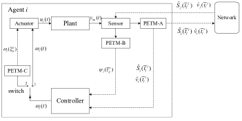
Figure 13: Modified control scheme.

References

References

- Behera, Bandyopadhyay, & Yu (2018) Behera, A., Bandyopadhyay, B., & Yu, X. (2018). Periodic event-triggered sliding mode control. Automatica, 96, 61-72.
- Bernuau, Moulay, Coirault, & Isfoula (2018) Bernuau, E., Moulay, E., Coirault, P., & Isfoula, F. (2019). Practical consensus of homogeneous sampled-data multi-agent systems. IEEE Transactions on Automatic Control, DOI: 10.1109/TAC.2019.2904442.
- Bin, Marconi, & Teel (2019) Bin, M., Marconi, L., & Teel, A. (2019). Adaptive output regulation for linear systems via discrete-time identifiers. Automatica, 105, 422-432.
- Cai, & Hu (2019) Cai, H., & Hu, G. (2019). Dynamic consensus tracking of uncertain Lagrangian systems with a switched command generator. IEEE Transactions on Automatic Control, DOI: 10.1109/TAC.2019.2893874.
- Cai, & Huang (2016) Cai, H., & Huang, J. (2016). The leader-following consensus for multiple uncertain Euler-Lagrange systems with an adaptive distributed observer. IEEE Transactions on Automatic Control, 61(10), 3152-3157.
- Cai, Lewis, Hu, & Huang (2017) Cai, H., Lewis, F., Hu, G., & Huang, J. (2017). The adaptive distributed observer approach to the cooperative output regulation of linear multi-agent systems. Automatica, 61, 299-305.
- Chen, & Chen (2017) Chen, X., & Chen, Z. (2017). Robust sampled-data output synchronization of nonlinear heterogeneous multi-agents. IEEE Transactions on Automatic Control, 62(3), 1458-1464.
- Chen, & Huang (2015) Chen, Z., & Huang, J. (2015). Stabilization and regulation of nonlinear systems: A robust and adaptive approach. Springer International Publishing Switzerland.
- Chen, & Sun (2020) Chen, C., & Sun, Z. (2020). A unified approach to finite-time stabilization of high-order nonlinear systems with an asymmetric output constraint. Automatica, 111, 108581.
- Cheng, & Ugrinovskii (2016) Cheng, Y., & Ugrinovskii, V. (2016). Event-triggered leader-following tracking control for multivariable multi-agent systems. Automatica, 70, 204-210.
- Cuenca, Antunes, Castillo, Garcia, Khashooei, & Heemels (2019) Cuenca, A., Antunes, D., Castillo, A., Garcia, P., Khashooei, B., & Heemels, W. (2019). Periodic event-triggered sampling and dual-rate control for a wireless networked control system with applications to UAVs. IEEE Transactions on Industrial Electronics, 66(4), 3157-3166.
- Deng, & Yang (2019) Deng, C., & Yang, G. (2019). Distributed adaptive fault-tolerant control approach to cooperative output regulation for linear multi-agent systems. Automatica, 103, 62-68.
- Franceschelli, Gasparri, Giua, & Seatzu (2013) Franceschelli, M., Gasparri, A., Giua, A., & Seatzu, C. (2013). Decentralized estimation of Laplacian eigenvalues in multi-agent systems. Automatica, 49(4), 1031-1036.
- Garcia, Cao, & Casbeer (2017) Garcia, E., Cao, Y., & Casbeer, D. (2017). Periodic event-triggered synchronization of linear multi-agent systems with communication delays. IEEE Transactions on Automatic Control, 62(1), 366-371.
- Hu, Liu, & Feng (2018) Hu, W., Liu, L., & Feng, G. (2018). Cooperative output regulation of linear multi-agent systems by intermittent communication: A unified framework of time and event-triggering strategies. IEEE Transactions on Automatic Control, 63(2), 548-555.
- Hu, Liu, & Feng (2019) Hu, W., Liu, L., & Feng, G. (2019). Event-triggered cooperative output regulation of linear multi-agent systems under jointly connected topologies. IEEE Transactions on Automatic Control, 64(3), 1317-1322.
- Li, Li, & Tong (2019) Li, Y., Li, K., & Tong, S. (2019). Finite-time adaptive fuzzy output feedback dynamic surface control for MIMO non-strict feedback systems. IEEE Transactions on Fuzzy Systems, vol.27, no.1, pp.96-110, 2019.
- Li, Qu, & Tong (2019) Li, Y., Qu, F., & Tong, S. (2019). Observer-based fuzzy adaptive finite time containment control of nonlinear multi-agent systems with input-delay. IEEE Transactions on Cybernetics, DOI: 10.1109/TCYB.2020.2970454.
- Li, Xing, Zhao, & Shi (2017) Li, L., Xing, W., Zhao, Y., & Shi, P. (2017). Stability analysis of multi-agent systems with multiple leaders of variable velocities based on consensus protocols. ICIC Express Letters, 11(11), 1599-1609.
- Liu, & Huang (2018) Liu, W., & Huang, J. (2018). Cooperative global robust output regulation for a class of nonlinear multi-agent systems by distributed event-triggered control. Automatica, 93, 138-148.
- Liu, & Huang (2019) Liu, W., & Huang, J. (2019). Leader-following consensus for linear multi-agent systems via asynchronous sampled-data control. IEEE Transactions on Automatic Control, DOI: 10.1109/TAC.2019.2948256.
- Liu, & Huang (2020) Liu, W., & Huang, J. (2020). Output regulation of linear systems via sampled-data control. Automatica, 113, 108684.
- Liu, & Huang (2019) Liu, T., & Huang, J. (2019). A distributed observer for a class of nonlinear systems and its application to a leader-following consensus problem. IEEE Transactions on Automatic Control, 64(3), 1221-1227.
- Liu, Ma, Lewis, & Wan (2019) Liu, H., Ma, T., Lewis, F., & Wan, Y. (2019). Robust formation trajectory tracking control for multiple quadrotors with communication delays. IEEE Transactions on Control Systems Technology, DOI: 10.1109/TCST.2019.2942277.
- Menard, Moulay, Coirault, & Defoort (2019) Menard, T., Moulay, E., Coirault, P., & Defoort, M. (2019). Observer-based consensus for second-order multi-agent systems with arbitrary asynchronous and aperiodic sampling periods. Automatica, 99, 237-245.
- Meng, Xie, & Soh (2017) Meng, X., Xie, L., & Soh Y. (2017). Asynchronous periodic event-triggered consensus for multi-agent systems. Automatica, 84, 214-220.
- Nowzari, Garcia, & Cortés (2019) Nowzari, C., Garcia E., & Cortés, J. (2019). Event-triggered communication and control of networked systems for multi-agent consensus. Automatica, 105, 1-27.
- Poveda, & Teel (2019) Poveda, J., & Teel, A. (2019). Hybrid mechanisms for robust synchronization and coordination of multi-agent networked sampled-data systems. Automatica, 99, 41-53.
- Shi, & Shen (2017) Shi, P., & Shen, Q. (2017). Observer-based leader-following consensus of uncertain nonlinear multi-agent systems. International Journal of Robust and Nonlinear Control, 27(17), 3794-3811.
- Singh, Tiwari, Garg (2018) Singh, A., Tiwari, V., & Garg, P. (2018). Anonymous decision logic for secure multi-agent computing. ICIC Express Letters Part B Applications, 9(12), 1217-1222.
- Stankovic, Stankovic, & Johansson (2018) Stankovic, M., Stankovic, S., & Johansson, K. (2018). Distributed time synchronization for networks with random delays and measurement noise. Automatica, 93, 126-137.
- Su (2019) Su, Y. (2019). Semi-global output feedback cooperative control for nonlinear multi-agent systems via internal model approach. Automatica, 103, 200-207.
- Sun, Hu, Xie, & Egerstedt (2018) Sun, C., Hu, G., Xie, L., & Egerstedt, M. (2018). Robust finite-time connectivity preserving coordination of second-order multi-agent systems. Automatica, 89, 21-27.
- Wang, Postoyan, Nesic, & Heemels (2019) Wang, W., Postoyan, R., Nesic, D., & Heemels, W. (2019). Periodic event-triggered control for nonlinear networked control systems. IEEE Transactions on Automatic Control, DOI: 10.1109/TAC.2019.2914255.
- Xing, Wen, Liu, Su, & Cai (2017) Xing, L., Wen, C, Liu, Z., Su, H., & Cai, J. (2017). Event-triggered adaptive control for a class of uncertain nonlinear systems. IEEE Transactions on Automatic Control, 62(4), 2107-2076.
- Xu, Yang, Wang, & Shu (2019) Xu, M., Yang, P., Wang, Y. & Shu, Q. (2019). Observer-based multi-agent system fault upper bound estimation and fault-tolerant consensus control. International Journal of Innovative Computing, Information and Control, 15(2), 519-534.
- Yang, & Liberzon (2018) Yang, G., & Liberzon, D. (2018). Feedback stabilization of switched linear systems with unknown disturbances under data-rate constraints. IEEE Transactions on Automatic Control, 63(7), 2107-2122.
- Yang, Sun, Zheng, & Li (2018) Yang, J., Sun, J., Zheng, W., & Li, S. (2018). Periodic event-triggered robust output feedback control for nonlinear uncertain systems with time-varying disturbance. Automatica, 94, 324-333.
- Yang, Zhang, Feng, Yan, & Wang (2019) Yang, R., Zhang, H., Feng, G., Yan, H., & Wang, Z. (2019). Robust cooperative output regulation of multi-agent systems via adaptive event-triggered control. Automatica, 102, 129-136.
- Zhang, Gao, & Kaynak (2013) Zhang, L., Gao, H., & Kaynak, O. (2013). Network-induced constraints in networked control systems-A survey. IEEE Transactions on Industrial Informatics, 9(1), 403-416.
- Zheng, Shi, Wang, & Shi (2019) Zheng, S., Shi, P., Wang, S., & Shi, Y. (2019). Event-triggered adaptive fuzzy consensus for interconnected switched multiagent systems. IEEE Transactions on Fuzzy Systems, 27(1), 144-158.
- Zhu, & Zheng (2019) Zhu, Y., & Zheng, W. (2020). Multiple Lyapunov functions analysis approach for discrete-time switched piecewise-affine systems under dwell-time constraints. IEEE Transactions on Automatic Control, 65(5), 2177-2184.
- Zhu, Zheng, & Zhou (2019) Zhu, Y., Zheng, W., & Zhou, D. (2020). Quasi-synchronization of discrete-time Lur’e-type switched systems with parameter mismatches and relaxed PDT constraints. IEEE Transactions on Cybernetics, 50(5), 2026-2037.