Adversarial Machine Learning:
Perspectives from Adversarial Risk Analysis

Abstract

Adversarial Machine Learning (AML) is emerging as a major field aimed at the protection of automated ML systems against security threats. The majority of work in this area has built upon a game-theoretic framework by modelling a conflict between an attacker and a defender. After reviewing game-theoretic approaches to AML, we discuss the benefits that a Bayesian Adversarial Risk Analysis perspective brings when defending ML based systems. A research agenda is included.

, , and

icmat]Institute of Mathematical Sciences, Spain (ICMAT-CSIC) samsi]The Statistical and Applied Mathematical Sciences Institute, NC, USA (SAMSI) duke]Department of Statistical Science, Duke University, NC, USA

1 Introduction

Over the last decade, an increasing number of processes are being automated through machine learning (ML) algorithms (Breiman,, 2001). It is essential that these algorithms are robust and reliable if we are to trust operations based on their output. State-of-the-art ML algorithms perform extraordinarily well on standard data, but have recently been shown to be vulnerable to adversarial examples, data instances targeted at fooling those algorithms (Goodfellow et al.,, 2015). The presence of adaptive adversaries has been pointed out in areas such as spam detection (Zeager et al.,, 2017); fraud detection (Kołcz and Teo,, 2009); and computer vision (Goodfellow et al.,, 2015). In those contexts, algorithms should acknowledge the presence of possible adversaries to defend against their data manipulations. Comiter, (2019) provides a review from the policy perspective showing how many AI societal systems, including content filters, military systems, law enforcement systems and autonomous driving systems (ADS), are susceptible and vulnerable to attacks. As a motivating example, consider the case of fraud detection (Bolton and Hand,, 2002). As ML algorithms are incorporated to such task, fraudsters learn how to evade them. For instance, they could find out that making a huge transaction increases the probability of being detected and start issuing several smaller transactions rather than a single large transaction.

As a fundamental underlying hypothesis, ML systems rely on using independent and identically distributed (iid) data for both training and testing. However, security aspects in ML, part of the field of adversarial machine learning (AML), question this iid hypothesis given the presence of adaptive adversaries ready to intervene in the problem to modify the data and obtain a benefit. These perturbations induce differences between the training and test distributions.

Stemming from the pioneering work in adversarial classification (AC) in Dalvi et al., (2004), the prevailing paradigm in AML to model the confrontation between learning-based systems and adversaries has been game theory (Menache and Ozdaglar,, 2011). This entails well-known common knowledge (CK) hypothesis (Hargreaves-Heap and Varoufakis,, 2004) which are doubtful in security applications as adversaries try to hide and conceal information.

As pointed out in Fan et al., (2019), there is a need for a principled framework that guarantees robustness of ML against adversarial manipulations in a principled way. In this paper we aim at formulating such framework. After providing an overview of key concepts and methods in AML emphasising the underlying game theoretic assumptions, we suggest an alternative formal Bayesian decision theoretic approach based on Adversarial Risk Analysis (ARA), illustrating it in supervised and reinforcement learning problems. We end up with a research agenda for the proposed framework.

2 Motivating examples

Two motivating examples serve us to illustrate key issues in AML.

2.1 Attacking computer vision algorithms

Vision algorithms are at the core of many AI systems such as ADS (Bojarski et al.,, 2016) and (McAllister et al.,, 2017). The simplest and most notorious attack examples to such algorithms consist of modifications of images in such a way that the alteration becomes imperceptible to the human eye, yet drives a model trained on millions of images to misclassify the modified ones, with potentially relevant security consequences.

Example.

With a relatively simple convolutional neural network model, we are able to accurately predict 99% of the handwritten digits in the MNIST data set (LeCun et al.,, 1998). However, if we attack those data with the fast gradient sign method in Szegedy et al., (2014), its accuracy is reduced to 62%. Figure 1 provides an example of an original MNIST image and a perturbed one. Although to our eyes both images look like a 2, our classifier rightly identifies a 2 in the first case (Fig. 1(a)), whereas it suggests a 7 after the perturbation (Fig. 1(b)).

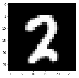
(a) Original image

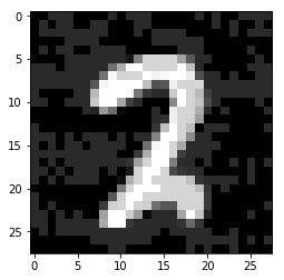
(b) Perturbed image

Figure 1: An original input and its attacked version.

$\triangle$

This type of attacks are easily built through low cost computational methods. However, they require the attacker to have precise knowledge about the architecture and weights of the corresponding predictive model. This is debatable in security settings, a main driver of this paper.

2.2 Attacking spam detection algorithms

Consider spam detection problems, an example of content filter systems. We employ the utility sensitive naive Bayes (NB) classifier, a standard spam detection approach (Song et al.,, 2009), studying its degraded performance under the 1 Good Word Insertion attacks in Naveiro et al., 2019a . In this case, the adversary just attacks spam emails adding to them a good word, that is, a word which is common in legit emails but not in spam ones.

Example.

We use the Spambase Data Set from the UCI ML repository (Lichman,, 2013). Accuracy and False Positive and Negative Rates are reported in Table 1, estimated via repeated hold-out validation over 100 repetitions (Kim,, 2009). We provide as well the standard deviation of each metric, also estimated through repeated hold-out validation.

	Accuracy	FPR	FNR
NB-Plain	$0.886\pm 0.009$	$0.680\pm 0.100$	$0.19\pm 0.02$
NB-Tainted	$0.761\pm 0.101$	$0.680\pm 0.100$	$0.500\pm 0.250$

Table 1: Performance of utility sensitive NB in clean and attacked data.

NB-Plain and NB-Tainted refer to results of NB on clean and attacked data, respectively. Observe how the presence of an adversary degrades NB accuracy: FPR coincides for NB-Plain and NB-Tainted as the adversary is not modifying innocent instances. However, false negatives undermine NB-Tainted performance, as the classifier is not able to identify a large proportion of attacked spam emails. $\triangle$

Both examples show how the performance of ML based systems may degrade under attacks. This suggests the need to take into account the presence of adversaries as done in AML.

3 Adversarial Machine Learning: a review

In this section, we present key results and concepts in AML. Further perspectives may be found in recent reviews by Vorobeychik and Kantarcioglu, (2018), Joseph et al., (2019), Biggio and Roli, (2018), Dasgupta and Collins, (2019) and Zhou et al., (2018). We focus on key ideas in the brief history of the field to motivate a reflection leading to our alternative approach in Sections 4 and 5. We remain at a conceptual level, with relevant modelling and computational ideas in Section 4.

3.1 Adversarial classification

Classification is one of the most widely used instances of supervised learning (Bishop,, 2006). Most efforts in this field have focused on obtaining more accurate algorithms which, however, have largely ignored the presence of adversaries who actively manipulate data to fool a classifier in search of a benefit. Dalvi et al., (2004) introduced adversarial classification (AC), a pioneering approach to enhance classification algorithms when an adversary is present. They view AC as a game between a classifier, also referred to as defender ($D$, she), and an adversary, ($A$, he). The classifier aims at finding an optimal classification strategy against $A$’s optimal attacks. Computing Nash equilibria (NE) in such general games quickly becomes very complex. Thus, they propose a forward myopic version in which D first assumes that the data is untainted, computing her optimal classifier; then, A deploys his optimal attack against it; subsequently, D implements the best response classifier against such attack, and so on. This approach assumes CK, or the assumption that all parameters of both players are known to each other. Although standard in game theory, this assumption is actually unrealistic in the security settings typical of AML.

Stemming from it, there has been an important literature in AC reviewed in Biggio et al., (2014) or Li and Vorobeychik, (2014). Subsequent approaches have focused on analyzing attacks over algorithms and upgrading their robustness against such attacks. To that end, strong assumptions about the adversary are typically made. For instance, Lowd and Meek, (2005) consider that the adversary can send membership queries to the classifier to issue optimal attacks, then proving the vulnerability of linear classifiers. A few methods have been proposed to robustify classification algorithms in adversarial environments, most of them focused on application-specific domains, as Kołcz and Teo, (2009) in spam detection. Vorobeychik and Li, (2014) study the impact of randomization schemes over classifiers against attacks proposing an optimal randomization defense. Other approaches have focused on improving Dalvi et al., (2004) model but, as far as we know, none got rid of the unrealistic CK assumptions. As an example, Kantarcıoğlu et al., (2011) use a Stackelberg game in which both players know each other’s payoff functions.

3.2 Adversarial prediction

An important source of AML cases are Adversarial Prediction Problems (APPs), Brückner and Scheffer, (2011).They focus on building predictive models where an adversary exercises some control over the data generation process, jeopardising standard prediction techniques. APPs model the interaction between the predictor and the adversary as a two agent game, a defender that aims at learning a parametric predictive model and an adversary trying to transform the distribution governing data at training time. The agents’ costs depend on both the predictive model and the adversarial data transformation. Both agents aim at optimizing their operational costs, which is a function of their expected losses under the perturbed data distribution. As this distribution is unknown, the agents actually optimize their regularized empirical costs, based on the training data. The specific optimization problem depends on the case considered.

First, in Stackelberg prediction games, Brückner and Scheffer, (2011) assume full information of the attacker about the predictive model used by the defender who, in addition, is assumed to have perfect information about the adversary’s costs and action space. $D$ acts first choosing her parameter; then, $A$, after observing this decision, chooses the optimal data transformation. Finding NE in these games requires solving a bi-level optimization problem, optimizing the defender’s cost function subject to the adversary optimizing his, after observing the defender’s choice. As nested optimization problems are intrinsically hard, the authors restrict to simple classes where analytical solutions can be found. On the other hand, in Nash prediction games (Brückner et al.,, 2012) both agents act simultaneously. The main concern is then seeking for NE. The authors provide conditions for their existence and uniqueness in specific classes of games.

3.3 Adversarial unsupervised learning

Much less AML work is available in relation with unsupervised learning. A relevant proposal is Kos et al., (2018) who describe adversarial attacks to generative models such as variational autoencoders (VAEs) or generative adversarial networks used in density estimation. Their focus is on slightly perturbing the input to the models so that the reconstructed output is completely different from the original input.

To the best of our knowledge, Biggio et al., (2013) first studied clustering under adversarial disturbances. They suggest a framework to create attacks during training that significantly alter cluster assignments, as well as an obfuscation attack that slightly perturbs an input to be clustered in a predefined assignment, showing that single-link hierarchical clustering is sensitive to these attacks.

Lastly, adversarial attacks on autoregressive (AR) models have started to attract interest. Alfeld et al., (2016) describe an attacker manipulating the inputs to drive the latent space of a linear AR model towards a region of interest. Papernot et al., (2016) propose adversarial perturbations over recurrent neural networks.

3.4 Adversarial reinforcement learning

The prevailing solution approach in reinforcement learning (RL) is $Q$-learning (Sutton et al.,, 1998). Deep RL has faced an incredible growth (Silver et al.,, 2017); however, the corresponding systems may be targets of attacks and robust methods are needed (Huang et al.,, 2017).

An AML related field of interest is multi-agent RL (Buşoniu et al.,, 2010). Single-agent RL methods fail in multi-agent settings, as they do not take into account the non-stationarity due to the other agents’ actions: $Q$-learning may lead to suboptimal results. Thus, we must reason about and forecast the adversaries’ behaviour. Several methods have been proposed in the AI literature (Albrecht and Stone,, 2018). A dominant approach draws on fictitious play (Brown,, 1951) and consists of assessing the other agents computing their frequencies of choosing various actions. Using explicit representations of the other agents’ beliefs about their opponents could lead to an infinite hierarchy of decision making problems, as explained in Section 5.3.

The application of these tools to $Q$-learning in multi-agent settings remains largely unexplored. Relevant extensions have rather focused on Markov games. Three well-known solutions are minimax-$Q$ learning (Littman,, 1994), which solves at each iteration a minimax problem; Nash-$Q$ learning (Hu and Wellman,, 2003), which generalizes to the non-zero sum case; or friend-or-foe-$Q$ learning (Littman,, 2001), in which the agent knows in advance whether her opponent is an adversary or a collaborator.

3.5 Adversarial examples

One of the most influential concepts triggering the recent interest in AML are adversarial examples. They were introduced by Szegedy et al., (2014) within neural network (NN) models, as perturbed data instances obtained through solving certain optimization problem. NNs are highly sensitive to such examples (Goodfellow et al.,, 2015).

The usual framework for robustifying models against these examples is adversarial training (AT) (Madry et al.,, 2018), based on solving a bi-level optimization problem whose objective function is the empirical risk of a model under worst case data perturbations. AT approximates the inner optimization through a projected gradient descent (PGD) algorithm, ensuring that the perturbed input falls within a tolerable boundary. The complexity of this attack depends on the chosen norm. However, recent pointers urge modellers to depart from using norm based approaches (Carlini et al.,, 2019) and develop more realistic attack models, as in Brown et al., (2017) adversarial patches.

3.6 The AML pipeline

The above subsections reviewed key developments in AML from a historical perspective. We summarise now the pipeline typically followed to improve security of ML systems (Biggio and Roli,, 2018).

Modelling threats.

This activity is critical to ensure ML security in adversarial environments. In general, we should assess three attacker features.

First, we should consider his goals, which vary depending on the setting, ranging from money to causing fatalities, going through damaging reputation (Couce-Vieira et al.,, 2019). Prior to deploying an ML system, it is crucial to guarantee its robustness against attackers with the most common goals. For instance, in fraud detection the attacker usually obfuscates fraudulent transactions to make the system classify them as legitimate ones in search of an economic benefit: a fraud detection system should be robust against such attacks. In general, these are classified following two criteria regarding their goals: violation type and attack specificity. For the first criterion, we distinguish between integrity violations, aimed at moving the prediction of particular instances towards the attacker’s target, e.g. have malicious samples misclassified as legitimate; availability violations, aimed at increasing the predictive error to make the system unusable; and privacy violations (a.k.a, exploratory attacks) to gain information about the ML system. In relation with the second one, we distinguish between targeted, which address just a few, even one, defenders, and indiscriminate attacks, affecting many defenders in a random manner.

Next, we consider that at the time of attacking, the adversary could have knowledge about different aspects of the ML system such as the training data used, or the features. Thus, we classify adversarial threats depending on which aspects is the attacker assumed to have knowledge about. At one end of the spectrum, we find white box or perfect knowledge attacks: the adversary knows every aspect of the ML system. This is almost never the case in actual scenarios, except perhaps for insiders. Yet they could be useful in sequential settings where the ML system moves first, training an algorithm to find its specific parameters. The adversary, who moves afterwards, has some time to observe the behaviour of the system and learn about it. At the other end, black box or zero knowledge attacks assume that the adversary has capabilities to query the system but does not have any information about the data, the feature space or the particular algorithms used. This is the most reasonable assumption in which attacking and defending decisions are eventually made simultaneously. In between attacks are called gray box or limited knowledge. This is the most common type of attacks in security settings, especially when attacking and defending decisions are made sequentially but there is private information that the intervening agents are not willing to share.

Finally, we classify the attacks depending on the capabilities of the adversary to influence on data. In some cases, he may obfuscate training data to induce errors during operation, called poisoning attacks. On the other hand, evasion attacks have no influence on training data, but perform modifications during operation, for instance when trying to evade a detection system. These data alteration or crafting activities are the typical ones in AML and we designate them as coming from a data-fiddler. But there could be attackers capable of changing the underlying structure of the problem, affecting process parameters, called structural attackers. Moreover, some adversaries could be making decisions in parallel to those of the defender with the agents’ losses depending on both decisions, which we term parallel attackers.

Simulating attacks.

The standard approach, Biggio and Roli, (2018), formalizes poisoning and evasion attacks in terms of constrained optimization problems with different assumptions about the adversary’s knowledge, goals and capabilities. In general, the objective function in such problems assesses attack effectiveness, taking into account the attacker’s goals and knowledge. The constraints frame assumptions such as the adversary wanting to avoid detection or having a maximum attacking budget.

Protecting learning algorithms.

Two types of defence methods have been proposed. Reactive defences aim to mitigate or eliminate the effects of an eventual attack. They include timely detection of attacks, e.g. Naveiro et al., 2019b ; frequent retraining of learning algorithms; or verification of algorithmic decisions by experts. Proactive defences aim to prevent attack execution. They can entail security-by-design approaches such as explicitly accounting for adversarial manipulations, e.g., Naveiro et al., 2019a , or developing provably secure algorithms against specific perturbations (e.g., Gowal et al., (2018)); or security-by-obscurity techniques such as randomization of the algorithm response, or gradient obfuscation to make attacks less likely to succeed (Athalye et al.,, 2018).

3.7 General comments

We have provided an overview of key concepts in AML. Practically all ML methodologies have been touched upon from an adversarial perspective including, to quote a few approaches not mentioned above, logistic regression (Feng et al.,, 2014); support vector machines (Biggio et al.,, 2012); or latent Dirichlet allocations (Mei and Zhu,, 2015). As mentioned, it is very relevant from an applied point of view in areas like national security and cybersecurity. Of major importance in AML is the cleverhans (Papernot et al.,, 2018) library, built on top of the tensorflow framework, aimed at accelerating research in developing new attack threats and more robust defences for deep neural models.

This is a difficult area which is rapidly evolving and leading to an arms race in which the community alternates a cycle of proposing attacks and implementing defences that deal with the previous ones (Athalye et al.,, 2018). Thus, it is important to develop sound techniques. Note though, that stemming from the pioneering Dalvi et al., (2004), most of AML research has been framed within a standard game theory approach pervaded by NE and refinements. However, these entail CK assumptions which are hard to maintain in the security contexts typical of AML applications. We could argue that CK is too commonly assumed. We propose a decision theoretic based methodology to solve AML problems, adopting an ARA perspective to model the confrontation between attackers and defenders mitigating questionable CK assumptions, Rios Insua et al., (2009) and Banks et al., (2015).

4 ARA templates for AML

ARA makes operational the Bayesian approach to games, Kadane and Larkey, (1982) and Raiffa, (1982), facilitating a procedure to predict adversarial decisions, simulating them to obtain forecasts and protecting the learning system, as we formalise in Section 4.4. We provide before a comparison of game-theoretic and ARA concepts over three template AML models associated, respectively, to white, black and gray box attacks. They constitute basic structures which may be simplified or made more complex, through removing or adding nodes, and combined to accommodate specific AML problems. In all models, there is a defender who chooses her decision $d\in\mathcal{D}$ and an attacker who chooses his attack $a\in\mathcal{A}$. In the AML jargon, the defender would be the learning system (or the organisation deploying it) and the decisions she makes could refer to the various choices required, including the data set used, the models chosen, or the algorithms employed to estimate the parameters. In turn, the attacker would be the attacking organisation (or their corresponding attacking system); his decisions refer to the data sets chosen to attack or the period at which he decides to make it, but could also refer to structural or parallel decisions as in Section 3.6. The involved agents are assumed to maximise expected utility (or minimise expected loss) (French and Rios Insua,, 2000).

We use bi-agent influence diagrams (BAIDS) (Banks et al.,, 2015) to describe the problems: they include circular nodes representing uncertainties; hexagonal utility nodes, modelling preferences over consequences; and, square nodes portraying decisions. The arrows point to decision nodes (meaning that such decisions are made knowing the values of predecessors) or chance and value nodes (the corresponding events or consequences are influenced by predecessors). Different colours suggest issues relevant to just one of the agents (white, defender; gray, attacker); striped ones are relevant to both agents.

4.1 Sequential defend-attack games

We start with sequential games. $D$ chooses her decision $d$ and, then, $A$ chooses his attack $a$, after having observed $d$. This exemplifies white-box attacks, as the attacker has full information of $D$’s action at the time of making his decision. As an example, a classifier chooses and estimates a parametric classification algorithm and an attacker, who has access to the specific algorithm, sends examples to try to fool the classifier. These games have received various names like sequential Defend-Attack (Brown et al.,, 2006) or Stackelberg (Gibbons,, 1992). Their BAID is in Figure 2. Arc $D$-$A$ reflects that $D$’s choice is observed by $A$. The consequences for both systems depend on an attack outcome $\theta\in\Theta$. Each agent has its assessment on the probability of $\theta$, which depends on $d$ and $a$, respectively called $p_{D}(\theta|d,a)$ and $p_{A}(\theta|d,a)$. Similarly, their utility functions are $u_{D}(d,\theta)$ and $u_{A}(a,\theta)$.

Figure 2: Basic two player sequential defend-attack game

The basic game theoretic solution does not require $A$ to know $D$’s judgements, as he observes her decisions. However, $D$ must know those of $A$, the CK condition in this case. For its solution, we compute both agents’ expected utilities at node $\Theta$: $\psi_{A}(a,d)=\int u_{A}(a,\theta)\,p_{A}(\theta|d,a)\,\mathop{}\!\mathrm{d}\theta$, and $\psi_{D}(a,d)=\int u_{D}(d,\theta)\,p_{D}(\theta|d,a)\,\mathop{}\!\mathrm{d}\theta$. Next, we find $a^{*}(d)=\operatorname*{\arg\max}_{a\in\mathcal{A}}\,\psi_{A}(d,a)$, $A$’s best response to $D$’s action $d$. Then, $D$’s optimal action is $d^{*}_{\text{GT}}=\operatorname*{\arg\max}_{d\in\mathcal{D}}\,\psi_{D}(d,a^{*}(d))$. The pair $\left(d^{*}_{\text{GT}},\,a^{*}(d^{*}_{\text{GT}})\right)$ is a NE and, indeed, a sub-game perfect equilibrium.

Example.

The Stackelberg game in Brückner and Scheffer, (2011), Section 3.2, modeling the confrontation in an APP is a particular instance in which costs are minimized with no uncertainty about the outcome $\theta$. $D$ chooses the parameters $d$ of a predictive model. $A$ observes $d$ and chooses the transformation, converting data ${\mathcal{T}}$ into $a({\mathcal{T}})$. Let $\widehat{c}_{i}(d,a(\mathcal{T}))$ be the (regularized) empirical cost of the $i$-th agent, $i\in\{A,D\}$. Then, they propose a pair $[d^{*},a^{*}({\mathcal{T}}(d^{*}))]$ solving

$$\operatorname*{\arg\min}_{d} \widehat{c}_{D}(d,a^{*}({\mathcal{T}}(d)))$$

s.t. $$a^{*}({\mathcal{T}}(d))\in\operatorname*{\arg\min}_{a({\mathcal{T}})}\widehat{c}_{A}(d,a({\mathcal{T}})),$$

which provides a NE. $\triangle$

Example.

Adversarial examples can be cast as well through sequential games. $A$ finds the best attack which leads to perturbed data instances obtained from solving the problem

$$\min_{\|\delta\|\leq\epsilon}\widehat{c}_{A}(h_{\theta}(a(x)),y),$$

with $a(x)=x+\delta$, a suitable perturbation of the original data instance $x$; $h_{\theta}(x)$, the output of a predictive model with parameters $\theta$; and $\widehat{c}_{A}(h_{\theta}(x),y)=-\widehat{c}_{D}(h_{\theta}(x),y)$, the cost of classifying $x$ as of being of class $h_{\theta}(x)$ when the actual label is $y$.

In turn, robustifying models against those perturbations through AT aims at solving the problem $\min_{\theta}\mathbb{E}_{(x,y)\sim\mathcal{D}}\left[\max_{\|\delta_{x}\|\leq\epsilon}\widehat{c}_{D}(h_{\theta}(a(x)),y)\right]$: we minimize the empirical risk of a model under worst case perturbations of the data $\mathcal{D}$. The inner maximization problem is solved through PGD, with iterations $x_{t+1}=\Pi_{B(x)}(x_{t}-\alpha\nabla_{x}\widehat{c}_{A}(h_{\theta}(x_{t}),y)),$ where $\Pi$ is a projection operator ensuring that the perturbed input falls within a tolerable boundary $B(x)$. After $T$ iterations, we make $a(x)=x_{T}$ and optimize with respect to $\theta$. Madry et al., (2018) argue that the PGD attack is the strongest one using only gradient information from the target model; however, there has been evidence that it is not sufficient for full defence of neural models (Gowal et al.,, 2018). The complexity of the above attack depends on the chosen norm; for instance, if we resort to small perturbations under $\ell_{\infty}$ norm, the update simplifies to $x:=x-\epsilon\,\mbox{sign}\nabla_{x}\widehat{c}_{A}(h_{\theta}(x),y),$ making it attractive because of its low computational burden. The $\ell_{2}$ norm can also be considered, leading to updates $x:=x-\epsilon\,\frac{\nabla_{x}\widehat{C}_{A}(h_{\theta}(x),y)}{\|\nabla_{x}\widehat{C}_{A}(h_{\theta}(x),y)\|_{2}}.$ $\triangle$

The above CK condition is weakened if we assume only partial information, leading to games under incomplete information (Harsanyi,, 1967), but we defer their discussion until Section 4.3. These CK conditions, and those used under incomplete information, are doubtful as we do not actually have available the attacker his judgements. Moreover, they could lack robustness to perturbations in such judgements, Ekin et al., (2019).

Alternatively, we perform a Bayesian decision theoretic approach based on ARA. We weaken the CK assumption: the defender does not know $(p_{A},u_{A})$ and faces the problem in Figure 3(a). To solve it, she needs $p_{D}(a|d)$, her assessment of the probability that $A$ will implement attack $a$ after observing $d$. Then, her expected utility would be $\psi_{D}(d)=\int\psi_{D}(a,d)\,p_{D}(a|d)\mathop{}\!\mathrm{d}a$ with optimal decision $d^{*}_{\text{ARA}}=\arg\max_{d\in\mathcal{D}}\psi_{D}(d)$. This solution does not necessarily correspond to a NE (both solutions are based on different information and assumptions).

(a) Decision problem seen by defender.

(b) Defender analysis of attacker problem.

Figure 3: Influence Diagrams for defender and attacker problems.

To elicit $p_{D}(a|d)$, $D$ benefits from modeling $A$’s problem, with his ID in Figure 3(b). For this, she would use all information available about $p_{A}$ and $u_{A}$; her uncertainty about $(p_{A},u_{A})$ is modelled through a distribution $F=(U_{A},P_{A})$ over the space of utilities and probabilities. This induces a distribution over $A$’s expected utility, where his random expected utility would be $\Psi_{A}(a,d)=\int U_{A}(a,\theta)P_{A}(\theta|a,d)\mathop{}\!\mathrm{d}\theta$. Then, $D$ would find $p_{D}(a|d)=\mathbb{P}_{F}\left[a=\operatorname*{\arg\max}_{x\in\mathcal{A}}\Psi_{A}(x,d)\right]$, in the discrete case and, similarly, in the continuous one. In general, we would use Monte Carlo (MC) simulation to approximate $p_{D}(a|d)$.

4.2 Simultaneous defend-attack games

Consider next simultaneous games: the agents decide their actions without knowing the one chosen by each other. Black-box attacks are assimilated to them. As an example, a defender fits a classification algorithm; an attacker, who has no information about it, sends tainted examples to try to outguess the classifier. Their basic template is in Fig. 4.

Figure 4: Basic two player simultaneous defend-attack game.

Suppose the judgements from both agents, $(u_{D},p_{D})$ and $(u_{A},p_{A})$ respectively, are disclosed. Then, both $A$ and $D$ know the expected utility that a pair $(d,a)$ would provide them, $\psi_{A}(d,a)$ and $\psi_{D}(d,a)$. A NE $(d^{*},a^{*})$ in this game satisfies $\psi_{D}(d^{*},a^{*})\geq\psi_{D}(d,a^{*})\,\,\,\forall\,d\in{\cal D}$ and $\psi_{A}(d^{*},a^{*})\geq\psi_{A}(d^{*},a)\,\,\,\forall\,a\in{\cal A}.$

Example.

Nash prediction games are particular instances of simultaneous defend-attack games with sure outcomes. As in an APP, agents minimize (regularized empirical) costs, $\widehat{c}_{D}(d,a({\mathcal{T}}))$ and $\widehat{c}_{A}(d,a({\mathcal{T}}))$, with $a({\mathcal{T}})$ being the attacked dataset. Under CK of both players’ cost functions, a NE $[d^{*},a^{*}({\mathcal{T}})]$ satisfies $d^{*}\in\arg\min_{d}\widehat{C}_{D}(d,a^{*}({\mathcal{T}}))$, $a^{*}({\mathcal{T}})\in\arg\min_{a({\mathcal{T}})}\widehat{C}_{A}(d^{*},a({\mathcal{T}})).$ $\triangle$

If utilities and probabilities are not CK, we may proceed modelling the game as one with incomplete information using the notion of types: each player will have a type known to him but not to the opponent, representing private information. Such type $\tau_{i}\in T_{i}$ determines the agent’s utility $u_{i}(d,\theta,\tau_{i})$ and probability $p_{i}(\theta|d,a,\tau_{i})$, $i\in\{A,D\}$. Harsanyi proposes Bayes-Nash equilibria (BNE) as their solutions, still under a strong CK assumption: the adversaries’ beliefs about types are CK through a common prior $\pi(\tau_{D},\tau_{A})$ (moreover, the players’ beliefs about other uncertainties in the problem are also CK). Define strategy functions by associating a decision with each type, $d:\tau_{D}\rightarrow d(\tau_{D})\in{\cal D},$ $a:\tau_{A}\rightarrow a(\tau_{A})\in{\cal A}$. $D$’s expected utility associated with a pair of strategies $(d,a)$, given her type $\tau_{D}\in T_{D}$, is

$$\psi_{D}(d(\tau_{D}),a,\tau_{D})=\int\int u_{D}(d(\tau_{D}),\theta,\tau_{D})p_{D}(\theta|d(\tau_{D}),a(\tau_{A}),\tau_{D})\pi(\tau_{A}|\tau_{D})\;\mathrm{d}\tau_{A}\mathrm{d}\theta.$$

Similarly, we compute the attacker’s expected utility $\psi_{A}(d,a(\tau_{A}),\tau_{A})$. Then, a BNE is a pair $(d^{*},a^{*})$ of strategy functions satisfying

$$\psi_{D}(d^{*}(\tau_{D}),a^{*},\tau_{D}) \geq\psi_{D}(d(\tau_{D}),a^{*},\tau_{D}), \forall\,\tau_{D}\,$$

$$\psi_{A}(d^{*},a^{*}(\tau_{A}),\tau_{A}) \geq\psi_{A}(d^{*},a(\tau_{A}),\tau_{A}), \forall\,\tau_{A}$$

for every $d$ and every $a$, respectively.

The common prior assumptions are still unrealistic in AML security contexts. We thus weaken them in supporting $D$. She should maximize her expected utility through

$$d^{*}=\operatorname*{arg\,max}_{d\in{\cal D}}\,\int\int u_{D}(d,\theta)p_{D}(\theta\mid d,a)\pi_{D}(a)d\theta da.$$ (1)

where $\pi_{D}(a)$ models her beliefs about the attacker’s decision $a$, which we need to assess. Suppose $D$ thinks that $A$ maximizes expected utility, $a^{*}=\operatorname*{\arg\max}_{a\in{\cal A}}\int\left[\int u_{A}(a,\theta)\right]p_{A}(\theta|d,a)\mathop{}\!\mathrm{d}\theta\pi_{A}(d)\mathop{}\!\mathrm{d}d$. In general, she will be uncertain about $A$’s $(u_{A},p_{A},\pi_{A})$ required inputs. If we model all information available to her about it through a probability distribution $F\sim(U_{A},P_{A},\Pi_{A})$, mimicking  (1), we propagate such uncertainty to compute the distribution

$$A\mid D\sim\operatorname*{\arg\max}_{a\in{\cal A}}\,\int\left[\int U_{A}(a,\theta)\;P_{A}(\theta\mid d,a)\mathop{}\!\mathrm{d}\theta\right]\,\Pi_{A}(D=d)\mathop{}\!\mathrm{d}d.$$ (2)

$(U_{A},P_{A})$ could be directly elicited from $D$. However, eliciting $\Pi_{A}$ may require further analysis leading to an upper level of recursive thinking: she would need to think about how $A$ analyzes her problem (this is why we condition in (2) by the distribution of $D$). In the above, in order for $D$ to assess (2), she would elicit $(U_{A},P_{A})$ from her viewpoint, and assess $\Pi_{A}(D)$ through the analysis of her decision problem, as thought by $A$. This reduces the assessment of $\Pi_{A}(D)$ to computing $D\mid A^{1}\sim\operatorname*{\arg\max}_{d\in{\cal D}}\,\int\int U_{D}(d,\theta)\;P_{D}(\theta\mid d,a)d\theta\,\,\Pi_{D}(A^{1}=a)\mathop{}\!\mathrm{d}a,$ assuming she is able to assess $\Pi_{D}(A^{1})$, where $A^{1}$ represents $A$’s random decision within $D$’s second level of recursive thinking. For this, $D$ needs to elicit $(U_{D},P_{D})\sim G$, representing her knowledge about how $A$ estimates $u_{D}(d,a)$ and $p_{D}(\theta|d,a)$, when she analyzes how the attacker thinks about her decision problem. Again, eliciting $\Pi_{D}(A^{1})$ might require further thinking from $D$, leading to a recursion of nested models, connected with the level-$k$ thinking concept in Stahl and Wilson, (1994), which would stop at a level in which $D$ lacks the information necessary to assess the corresponding distributions. At such point, she could assign a non-informative distribution (French and Rios Insua,, 2000). Further details may be seen in Rios and Rios Insua, (2012).

4.3 Sequential defend-attack games with private information

Our final template is the sequential Defend-Attack model with defender private information. Gray-box attacks are assimilated to them. As an example, a defender estimates the parameters of a classification algorithm and an attacker, with no access to the algorithm but knowing the data used to train it, sends examples to try to fool the classifier. Fig. 5 depicts the template, with private information represented by $V$. Arc $V-D$ reflects that $v$ is known by $D$ when she makes her decision; the lack of arc $V-A$, that $v$ is not known by $A$ when making his decision. The uncertainty about the outcome $\theta$ depends on the actions by $A$ and $D$, as well as on $V$. The utility functions are $u_{D}(d,\theta,v)$ and $u_{A}(a,\theta,v)$.

Figure 5: Basic template for sequential defend-attack game with private information.

Standard game theory solves this model as a signaling game (Aliprantis and Chakrabarti,, 2002). For a more realistic approach, we weaken the required CK assumptions. Assume for now that $D$ has assessed $p_{D}(\theta|d,a,v)$, $u_{D}(d,\theta,v)$ and $p_{D}(a|d)$. Then, she obtains her optimal defence through

• At node $\Theta$, compute for each $(d,a,v)$, $\psi_{D}(d,a,v)=\int u_{D}(d,\theta,v)\;p_{D}(\theta\mid d,a,v)\;\mathrm{d}\theta.$

• At node $A$, compute $(d,v)\rightarrow\psi_{D}(d,v)=\int\psi_{D}(d,a,v)\;p_{D}(a\mid d)\;\mathrm{d}a$

• At node $D$, solve $v\rightarrow d^{*}(v)=\operatorname*{arg\,max}_{d\in{\cal D}}\,\psi_{D}(d,v).$

To assess $p_{D}(a|d)$, $D$ could solve $A$’s problem from her perspective. As $A$ does not know $v$, his uncertainty is represented through $p_{A}(v)$, describing his (prior) beliefs about $v$. Arrow $V-D$ can be inverted to obtain $p_{A}(v|d)$. Note that we would still need to assess $p_{A}(d|v)$ for this. Should $D$ know $A$’s utility function $u_{A}(a,\theta,v)$ and probabilities $p_{A}(\theta|d,a,v)$ and $p_{A}(v|d)$, she would anticipate his attack $a^{*}(d)$ for any $d\in{\cal D}$ by

• At node $\Theta$, compute for each $(d,a,v)$, $\psi_{A}(d,a,v)=\int u_{A}(d,\theta,v)\;p_{i}(\theta\mid d,a,v)\;\mathrm{d}\theta$.

• At node $V$, compute for each $(d,a),$ $\psi_{A}(d,a)=\int\psi_{A}(d,a,v)\;p_{A}(v\mid d)\;\mathrm{d}v$.

• At node $A$, solve $d\rightarrow a^{*}(d)=\operatorname*{arg\,max}_{a\in{\cal A}}\,\psi_{A}(d,a).$

However, $D$ does not know $(p_{A},u_{A})$. She has beliefs about them, say $F\sim(P_{A},U_{A})$, which induce distributions $\Psi_{A}(d,a,v)$ and $\Psi_{A}(d,a)$ on $A$’s expected utilities through

$$\Psi_{A}(d,a,v)=\int U_{A}(a,\theta,v)\;P_{A}(\theta\mid d,a,v)\;\mathrm{d}\theta,\,\,\,\,\Psi_{A}(d,a)=\int\Psi_{A}(d,a,v)\;P_{A}(v\mid d)\;\mathrm{d}v.$$

Then, $D$’s predictive distribution about $A$’s response to her defense choice $d$ would be defined through

$$p_{D}(a|d)=P_{F}\Big{[}a=\operatorname*{\arg\max}_{x\in{\cal A}}\,\Psi_{A}(d,x)\Big{]},\;\forall a\in{\cal A}.$$

To sum up, the elicitation of $\left(P_{A}(\theta|d,a,v),P_{A}(v|d),U_{A}(a,\theta,v)\right)$ allows the defender to solve her problem of assessing $p_{D}(a|d)$. The defender may have enough information to directly assess $P_{A}(\theta|d,a,v)$ and $U_{A}(a,\theta,v)$. Yet the assessment of $P_{A}(v|d)$ requires a deeper analysis, since it has a strategic component, and would lead to a recursion as in Section 4.2, as detailed in Rios and Rios Insua, (2012).

4.4 A decision theoretic pipeline for AML

Based on the three templates, we revisit now the AML pipeline in Section 3.6 proposing an ARA based decision theoretic approach with the same steps.
1. Model system threats. This entails modelling the attacker problem from the defender perspective through an influence diagram (ID). The attacker key features are his goals, knowledge and capabilities. Assessing these require determining which are the actions that he may undertake and the utility that he perceives when performing a specific action, given a defender’s strategy. The output is the set of attacker’s decision nodes, together with the value node and arcs indicating how his utility depends on his decisions and those of the defender. Assessing the attacker knowledge entails looking for relevant information that he may have when performing the attack, and his degree of knowledge about this information, as we do not assume CK. This entails not only a modelling activity, but also a security assessment of the ML system to determine which of its elements are accessible to the attacker. The outputs are the uncertainty nodes of the attacker ID, the arcs connecting them and those ending in the decision nodes, indicating the information available to $A$ when attacking. Finally, identifying his capabilities requires determining which part of the defender problem the attacker has influence on. This provides the way the attacker ID connects with that of the defender.
2. Simulating attacks. Based on step 1, a mechanism is required to simulate reasonable attacks. The state of the art solution assumes that the attacker will be acting NE, given strong CK hypothesis. The ARA methodology relaxes such assumptions, through a procedure to simulate adversarial decisions. Starting with the adversary model (step 1), our uncertainty about his probabilities and utilities is propagated to his problem and leads to the corresponding random optimal adversarial decisions which provide the required simulation.
3. Adopting defences. In this final step, we augment the defender problem incorporating the attacker one produced in step 1. As output, we generate a BAID reflecting the confrontation big picture. Finally, we solve the defender problem maximizing her subjective expected utility, integrating out all attacker decisions, which are random from the defender perspective given the lack of CK. In general, the corresponding integrals are approximated through MC, simulating attacks consistent with our knowledge level about the attacker using the mechanism of step 2.

5 AML from an ARA perspective

We illustrate now how the previous templates can be combined and adapted through the proposed pipeline to provide support to AML models.

5.1 Adversarial supervised learning

Almost every supervised ML problem entails the tasks reflected in Figure 6: an inference (learning) stage, in which relevant information is extracted from training data $\mathcal{T}$, and a decision (operational) stage, in which a decision $y_{D}$ is made based on the gathered information.

Figure 6: Influence diagram for a supervised learning problem

In a general supervised learning problem under a Bayesian perspective, the first stage requires computing the posterior $p(\beta|\mathcal{T})\propto p(\beta)p(\mathcal{T}|\beta)$, where $p(\beta)$ is the prior on the model parameters; ${\mathcal{T}}$, the data; and $p(\mathcal{T}|\beta)$ the likelihood. Based on it, the predictive distribution is $p(y|x,\mathcal{T})=\int p(y|x,\beta)p(\beta|\mathcal{T})\mathop{}\!\mathrm{d}\beta.$ At the second stage, given an input $x$, the response $y_{D}$ has to be decided. If the actual value is $y$, the attained utility is $u_{D}(y,y_{D})$ and, globally, the expected utility is

$$\psi(y_{D}|x,\mathcal{T})=\int_{y}u_{D}(y,y_{D})p(y|x,\mathcal{T})\mathop{}\!\mathrm{d}y=\int_{y}u_{D}(y,y_{D})\left[\int p(y|x,\beta)p(\beta|\mathcal{T})\mathop{}\!\mathrm{d}\beta\right]\mathop{}\!\mathrm{d}y.$$

We aim at finding $\operatorname*{\arg\max}_{y_{D}}\psi(y_{D}|x,\mathcal{T})$.

An attacker might be interested in modifying the inference stage, through poisoning attacks, and/or the decision stage, through evasion attacks. Figure 7 represents both possibilities (step 3). In it, $\mathcal{T}^{\prime}$ denotes the poisoned data and $a_{T}$, the poisoning attack; $a_{O}$ denotes the evasion attack decision and $x^{\prime}$, the attacked feature vector actually observed by the defender. Finally, $u_{A}$ designates the attacker’s utility function.

Figure 7: Influence diagram for a generic adversarial supervised learning problem

If we just consider evasion attacks, $a_{T}$ is the identity, $\mathcal{T}^{\prime}=\mathcal{T}$, and inference will be as in Figure 6; when considering only poisoning attacks, $a_{O}$ would be the identity, the observed instance $x^{\prime}$ will coincide with $x$, and the decision stage is that in Figure 6. Assume that attacks are deterministic transformations of data: applying an attack to a given input will always lead to the same output.

Suppose the defender is not aware of the presence of the adversary. Then, she would receive the training data $\mathcal{T}^{\prime}$, use the posterior $p(\beta|\mathcal{T}^{\prime})$, compute the predictive $p(y|x,\mathcal{T^{\prime}})$, receive the data $x^{\prime}$ at operation time and solve $\operatorname*{\arg\max}_{y_{D}}\psi_{D}(y_{D}|x^{\prime},{\cal T}^{\prime})$. This will typically differ from $\operatorname*{\arg\max}_{y_{D}}\psi_{D}(y_{D}|x,{\cal\mathcal{T}})$, leading to an undesired performance degradation as shown in Section 2. Should the defender know how she has been attacked, and assuming that attacks are invertible, she would know $a_{O}^{-1}(x^{\prime})$ and $a_{T}^{-1}({\cal T}^{\prime})$ and maximise $\psi_{D}(y_{D}|a^{-1}_{O}(x^{\prime}),a_{T}^{-1}({\cal T}^{\prime}))$. However, she will not typically know neither the attacks, nor the original data. Thus, upon becoming adversary aware, she would deal with the problem in Figure 8, where now $A$’s decisions appear as random.

Figure 8: Supervised learning from the defender’s perspective

In such case, if her uncertainty is modelled through $p(a_{T}|{\cal T^{\prime}})$ and $p(a_{O}|x^{\prime})$, the defender would optimise

$$\int\left[\int\psi_{D}(y_{D}|a^{-1}_{O}(x^{\prime}),a_{T}^{-1}({\cal T}^{\prime}))p(a_{T}|{\cal T^{\prime}})da_{T}\right]p(a_{O}|x^{\prime})da_{O}.$$ (3)

We describe a procedure to assess the required distributions following the methodology in Section 4.4. To that end, (step 1) considers the problem that the attacker would be solving; (step 2) assesses our uncertainty about his problem to simulate from it; then, (step 3) the optimal defence (3) is proposed.

The attacker aims at modifying data to maximize his utility $u_{A}(y_{D},y,a_{T},a_{O})$, that depends on $y_{D}$, $y$, and the attacks $a_{T}$ and $a_{O}$, as these may have implementation costs. The form of his utility function depends on his goals, 3.6. Given that the adversary observes $(\mathcal{T},x,y)$, if we assume that he aims at maximising expected utility when trying to confuse the defender, he would find his best attacks through

$$\max_{a_{T},a_{O}}\int u_{A}(y_{D},y,a_{T},a_{O})p_{A}(y_{D}|a_{O}(x),a_{T}(\mathcal{T}))\mathop{}\!\mathrm{d}y,$$ (4)

where $p_{A}(y_{D}|a_{O}(x),a_{T}(\mathcal{T}))$ describes the probability that the defender says $y_{D}$ if she observes the training data $a_{T}(\mathcal{T})$ and features $a_{O}(x)$, from the adversary’s perspective. At this point, $D$ must model her uncertainty about $A$’s utilities and probabilities. She will use random utilities $U_{A}$ and probabilities $P_{A}$ and look for the random optimal adversarial transformations

$$(A_{T},A_{O})^{*}(\mathcal{T},x,y)=\arg\max_{a_{T},a_{O}}\int U_{A}(y_{D},y,a_{T},a_{O})P_{A}(y_{D}|a_{O}(x),a_{T}(\mathcal{T}))\mathop{}\!\mathrm{d}y.$$ (5)

Finally, she computes the probability of the attacker choosing attacks $a_{T}$ and $a_{O}$ when observing $\mathcal{T},x,y$ as

$$p(a_{T},a_{O}|\mathcal{T},x,y)=\mathbb{P}\left[(A_{T},A_{O})^{*}(\mathcal{T},x,y)=(a_{T},a_{O})\right].$$ (6)

Using this, she would compute the required quantities $p(a_{T}|{\cal T^{\prime}})$ and $p(a_{O}|x^{\prime})$.

This last step is problem dependent. We illustrate some specificities through an application to AC under evasion attacks.

5.2 Adversarial classification. An ARA perspective

Naveiro et al., 2019a introduce ACRA, an approach to AC from an ARA perspective. This is an application of the sketched framework to binary classification problems with malicious ($+$) and benign ($-$) labels. ACRA considers only evasion attacks ($a_{T}=id$) that are integrity violations, thus exclusively affecting malicious examples. To unclutter notation, we remove the dependence on training data $\mathcal{T}$, clean by assumption. In addition, we eliminate the subscript in evasion attacks and refer to them as $a$.

Figure 9(a) represents the problem faced by the defender. This BAID is the same as in Figure 8, removing the inference phase, standard by assumption.

(a) Classifier problem

(b) Adversary problem

Figure 9:

$D$ aims at choosing the class $y_{D}$ with maximum posterior expected utility based on the observed instance $x^{\prime}$: she must find $c(x^{\prime})=\operatorname*{\arg\max}_{y_{D}}\sum_{y\in\{+,-\}}u_{D}(y_{D},y)p_{D}(y|x^{\prime})$. Under the assumed type of attacks, this problem is equivalent to

$$c(x^{\prime})=\operatorname*{\arg\max}_{y_{D}}\bigg{[}u_{D}(y_{D},+)p_{D}(+)\sum_{x\in\mathcal{X}^{\prime}}p_{D}(a_{x\rightarrow x^{\prime}}|x,+)p_{D}(x|+)+u_{D}(y_{D},-)p_{D}(x^{\prime}|-)p_{D}(-)\bigg{]},$$ (7)

where $\mathcal{X}^{\prime}$ is the set of potentially originating instances $x$ leading to $x^{\prime}$ and $p_{D}(a_{x\rightarrow x^{\prime}}|x,+)$ designates the probability that $A$ will launch an attack that transforms $x$ into $x^{\prime}$, when he receives $(x,y=+)$, according to $D$. All required elements are standard except for $p_{D}(a_{x\rightarrow x^{\prime}}|x,y)$, which demands strategic thinking from $D$.

To make the approach operational, consider $A$’s decision making, Figure 9(b). Let $u_{A}(y_{D},y,a)$ be $A$’s utility when $D$ says $y_{D}$, the actual label is $y$ and the attack is $a$; and $p=p_{A}(c(a(x))=+|a(x))$, the probability that $A$ concedes to $D$ saying the instance is malicious, given that she observes $x^{\prime}=a(x)$. He will have uncertainty about it; denote its density $f_{A}(p|a(x))$ with expectation $p_{a(x)}^{A}$. Among all attacks, $A$ would choose

$$a^{*}(x,y)=\operatorname*{\arg\max}_{a}\int\bigg{[}u_{A}(c(a(x))=+,y,a)\cdot p\\ +u_{A}(c(a(x))=-,y,a)\cdot(1-p)\,\bigg{]}f_{A}(p|a(x))dp.$$

Under integrity violation attacks, we only consider the case $y=+$. $A$’s expected utility, when he adopts attack $a$ and the instance is $(x,y=+)$, is $[u_{A}(+,+,a)-u_{A}(-,+,a)]p_{a(x)}^{A}+u_{A}(-,+,a)$. However, $D$ does not know the ingredients $u_{A}$ and $p_{a(x)}^{A}$. If her uncertainty is modelled through a random utility function $U_{A}$ and a random expectation $P_{a(x)}^{A}$, the random optimal attack is

$$A^{*}(x,+)=\operatorname*{\arg\max}_{a}\bigg{(}\left[U_{A}(+,+,a)-U_{A}(-,+,a)\right]P_{a(x)}^{A}+U_{A}(-,+,a)\bigg{)},$$

and $p_{D}(a_{x\rightarrow x^{\prime}}|x,+)=Pr(A^{*}(x,+)=a_{x\rightarrow x^{\prime}})$, which may be estimated using MC. This would then feed problem (7).

Example.

Applying the ACRA framework to the spam detection example in Section 2.2, leads to the results in Table 2. Observe that ACRA is robust to attacks and identifies most of the spam. Its overall accuracy is above $0.9$, identifying most non-spam emails as well. ACRA presents smaller FNR than NB-Tainted and significantly lower FPR than NB, causing the overall performance to raise up.

	Accuracy	FPR	FNR
ACRA	$0.919\pm 0.010$	$0.019\pm 0.008$	$0.177\pm 0.022$
NB-Plain	$0.886\pm 0.009$	$0.680\pm 0.100$	$0.19\pm 0.02$
NB-Tainted	$0.761\pm 0.101$	$0.680\pm 0.100$	$0.500\pm 0.250$

Table 2: Performance comparison of ACRA and utility sensitive Naive Bayes.

$\triangle$

Interestingly, ACRA beats NB-Untainted in accuracy. This effect was observed in Dalvi et al., (2004) and Goodfellow et al., (2015) in different settings. The latter argues that taking into account the presence of an adversary has a regularizing effect improving the original accuracy of the underlying algorithm, making it more robust.

5.3 Adversarial reinforcement learning. An ARA perspective

Section 3.4 described how the presence of other agents may make non-stationary the environment in RL, rendering $Q$-learning ineffective. To properly deal with the problem, consider the extension of the simultaneous game in Section 4.2 to multiple stages, Figure 10. Figure 11 represents the problem from the perspective of just the defender.

Figure 10: Multi-agent RL problem.

Figure 11: Defender view on multi-agent RL.

To deal with this problem, the Markov Decision Process framework (Howard,, 1960) has to be augmented to account for the presence of adversaries. Consider the case of one agent (DM, $D$) facing just one opponent ($A$). A Threatened Markov Decision Process (TMDP) (Gallego et al., 2019a, ; Gallego et al., 2019b, ) is a tuple $\left(\Theta,\mathcal{D},\mathcal{A},\mathcal{P},u_{D},p_{D}\right)$ such that $\Theta$ designates the state space; $\mathcal{D}$ denotes the set of actions $d$ available to the supported agent; $\mathcal{A}$ designates the set of actions $a$ available to the adversary; $\mathcal{P}:\Theta\times\mathcal{D}\times\mathcal{A}\rightarrow\Delta(\Theta)$ is the transition distribution; $u_{D}:\Theta\times\mathcal{D}\times\mathcal{A}\rightarrow\Delta(\mathbb{R})$ is $D$’s utility distribution (denoted reward in the RL literature); and $p_{D}(a|\theta)$ models $D$’s beliefs about his opponent moves given the state $\theta\in\Theta$.

The effect of averaging over opponent actions is translated to the sequential setting, extending the $Q$-learning iteration to

$$Q(\theta,d,a):=(1-\alpha)Q(\theta,d,a)+\alpha\left(u_{D}(\theta,d,a)+\gamma\max_{d}\mathbb{E}_{p_{D}(a|\theta^{\prime})}\left[Q(\theta^{\prime},d,a)\right]\right)$$ (8)

and its expectation, $Q(\theta,d):=\mathbb{E}_{p_{D}(a|\theta)}\left[Q(\theta,d,a)\right]$. This is used to compute an $\epsilon-$greedy policy for the DM, i.e., choosing with probability $(1-\epsilon)$ an action $d^{*}=\operatorname*{\arg\max}_{d}\left[Q(\theta,d)\right]$, or, with probability $\epsilon$, a uniformly random action. The previous rule provides a fixed point of a contraction mapping, leading to a defender’s optimal policy, assuming her opponent behaviour is described by $p_{D}(a|\theta)$. Thus, it is key to model the uncertainty regarding the adversary’s policy through this distribution. In Gallego et al., 2019a we use a level-$k$ scheme, Section 4.2, to learn the opponent model: both agents maximize their respective expected cumulative utilities, though we start with a case in which the adversary is considered non-strategic. Then, we also consider the adversary being a level-1 agent and the DM a level-2 one. Gallego et al., 2019b goes up in the level-$k$ hierarchy considering also mixtures of opponents whose beliefs can be dynamically adapted by the DM. In most situations, $D$ will not know which type of opponent she is facing. For this, she can place a prior $p_{D}(M_{i})$ modeling her beliefs about her opponent using model $M_{i}$, $i=1,\ldots,m$, with $\sum_{i=1}^{m}p_{D}(M_{i})=1,p_{D}(M_{i})\geq 0$. As an example, she might place a Dirichlet prior. At each iteration, after having observed $a$, she updates her beliefs $p(M_{i})$ increasing the count of the model causing that action, as in a standard Dirichlet-Categorical model. For this, the defender maintains an estimate $p_{M_{i}}(a|s)$ of the opponent’s policy for each model $M_{i}$.

Example.

Consider the benefits of opponent modelling in a repeated matrix game, specifically the iterated variant of the Chicken game (IC), with payoff matrix in Table 3. For example, if the row agent plays $C$ and the column one plays $E$, the agents respectively obtain utilities of $-2$ and $1$. This game has two pure NE $(C,E)$ and $(E,C)$.

	$C$	$E$
$C$	(0, 0)	(-2, 1)
$E$	(1, -2)	(-4, -4)

Table 3: Payoff Matrix of Chicken

Fig. 12(a) depicts the utilities obtained over time by players, when both agents are modelled as independent $Q$-learners (they use the standard $Q$-function from RL as learning rule). Observe the ill convergence due to lack of opponent awareness. As mentioned in Section 3.4, when other agents interfere with a DM’s rewards, the environment can become non-stationary and $Q$-learning leads to suboptimal results (Buşoniu et al.,, 2010).

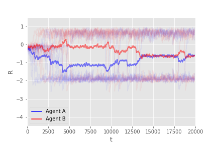
(a) Q-learner vs Q-learner

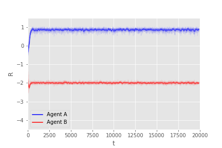
(b) L1 Q-learner (blue) vs Q-learner (red)

Figure 12: Rewards in IC game.

Alternatively (Fig. 12(b)), the DM with opponent modelling, based on (8) to estimate the opponent’s actions with historical frequencies, has an advantage and converges to her optimal Nash equilibrium $(E,C)$. $\triangle$

6 Conclusions: A research agenda

We have provided a review of key approaches, models and concepts in AML. This area is of major importance in security and cybersecurity to protect systems increasingly based on ML algorithms, Comiter, (2019). The pioneering AC work by Dalvi et al., (2004) has framed most of this research within the game-theoretic realm, with entailed CK conditions which actually hardly hold in the security contexts typical of AML. Our ARA alternative framework does not entail such conditions, being therefore much more realistic. As a byproduct, we obtain more robust algorithms. We illustrated their application in adversarial supervised learning, AC and RL problems. We end up providing several lines for further research.

6.1 Robustifying ML algorithms through Bayesian ideas

We argued how Bayesian methods provide enhanced robustness in AML. Ekin et al., (2019) shows how game theory solutions based on point estimates of preferences and beliefs, potentially lead to unstable solutions, while ARA solutions tend to be more robust acknowledging uncertainties in such judgements. Here are some additional ideas.
Bayesian methods and AML. It has been empirically shown that model ensembling is an effective mechanism for designing powerful attack models (Tramèr et al.,, 2018). The Bayesian treatment of ML models offers a way of combining the predictions of different models via the predictive distribution. Gal and Smith, (2018) show how certain idealized Bayesian NNs properly trained lack adversarial examples. Thus, a promising research line consists of developing efficient algorithms for approximate Bayesian inference with robustness guarantees.

Indeed, there are several ways in which the Bayesian approach may increase security of ML systems. Regarding opponent modelling, in sequential decision making, an agent has uncertainty over her opponent type initially; as information is gathered, she might be less uncertain about her model via Bayesian updating (Gallego et al., 2019b, ). Uncertainty over attacks in supervised models can also be considered to obtain a more robust version of AT, as in Ye and Zhu, (2018) who sample attacks using a SG-MCMC method. Combining their approach with ARA opponent modelling may further increase robustness. Lastly, there are alternative approaches to achieve robustness in presence of outliers and perturbed observations, as through the robust divergences for variational inference (Futami et al.,, 2018).
Robust Bayesian methods. The robust Bayesian literature burgeoned in the period 1980-2000 (Berger,, 1982; Rios Insua and Ruggeri,, 2000). In particular, there has been relevant work in Bayesian likelihood robustness (Shyamalkumar,, 2000) referring to likelihood imprecision, reminiscent of the impact of attacks over the data received. Note that Bayesian likelihood robustness focuses around random or imprecise perturbations and contaminations in contrast to the purposeful perturbations in AML. Not taking into account the presence of an adversary affecting data generation is an example of model mispecification; robustness of Bayesian inference to such issue has been revisited recently in Miller and Dunson, (2019). Their ideas could be used to robustify ML algorithms in adversarial contexts.

6.2 Modelling and computational enhancements

We discuss modelling and computational enhancements aimed at improving operational aspects of the proposed framework.
Characterizing attacks. A core element in the AML pipeline is the choice of the attacker perturbation domain. This is highly dependent on the nature of the data attacked. In computer vision, a common choice is an $\ell_{p}$ ball of radius $\delta$ centered at the original input. For instance, an $\ell_{\infty}$ norm implies that an attacker may modify any pixel by at most $\delta$. These perturbations, imperceptible to the human eye, may not be representative of threats actually deployed. As an example, Brown et al., (2017) designed a circular sticker that may be printed and deployed to fool state of the art classifiers. Thus, it is important to develop threat models that go beyond $\ell_{p}$ norm assumptions. Moreover, we discussed only problems with two agents. It is relevant to deal with multiple agents in several variants (one defender vs. several attackers, several defenders vs. several attackers) including cases in which agents on one of the sides somehow cooperate.
New algorithmic approaches. Exploring gradient-based techniques for bi-level optimization problems arising in AML is a fruitful line of research (Naveiro and Insua,, 2019). However the focus has been on white box attacks. It would be interesting to extend those results to the framework here proposed. On the other hand, Bayesian methods are also hard to scale to high dimensional problems or large datasets. Recent advances in accelerating SG-MCMC samplers, e.g., Gallego and Insua, (2019, 2018), are crucial to leverage the benefits of a Bayesian treatment.
Single stage computations. The framework proposed in Sections 4 and 5 essentially goes through simulating from the attacker problem to forecast attacks and then optimize for the defender to find her optimal decision. This may be computationally demanding and we could explore single stage approaches to alleviate computations. Initial ideas based on augmented probability simulation are in Ekin et al., (2019).

6.3 Adversarial machine learning methods

As mentioned in Section 4, our approach could be used to study adversarial versions of ML problems (classification, regression, unsupervised learning and RL). We are particularly interested in the following.
Adversarial classification. A main limitation of ACRA, Section 5.2, is the requirement of computing the conditional probabilities $p(x|y)$: this is only compatible with explicit generative models, such as Naive Bayes. This model can be weak as it does not account for feature correlations. A straightforward extension can be using a deep Bayes classifier with a VAE. Likewise, extensions to discriminative models and multi-class problems is on-going.
Unsupervised learning. Further research is required. As for non-hierarchical methods such as $k$-means clustering, we could treat $f(x)=\operatorname*{\arg\max}_{y}\|x-\mu_{y}\|^{-1}$ as a score function, so standard evasion techniques (Section 3) could straightforwardly be applied. Security of AR models (Alfeld et al.,, 2016) and natural language models (Wang et al.,, 2019) are attracting attention, so custom defences tailored to these models are in need.

6.4 Applications

As presented in Comiter, (2019), applications abound. We mention five of interest to us.
Fake news. The rise in computer power used in deep learning is leading to quasi-realistic automatic text generation (Radford et al.,, 2019), which can be used for malicious purposes such as fake reviews generation (Juuti et al.,, 2018). At present, state of the art defences consist mostly of statistical analyses of token distributions (Gehrmann et al.,, 2019). These are attacker-agnostic. An ARA treatment may be beneficial to inform the model of which are the most likely attack patterns.
Autonomous driving systems. ADS directly benefit from developments in computer vision and RL. However, accidents still occur because of lack of guarantees in verifying the correctness of deep NNs. Alternative solutions include the use of Bayesian NNs, as there is evidence that uncertainty measures can predict crashes up to five seconds in advance (Michelmore et al.,, 2018). McAllister et al., (2017) propose propagating the uncertainty over the network to achieve a safer driving style. As mentioned, adversaries may interact with the visual system through adversarial examples. Thus, developing stronger defences are of major importance.
Forecasting time series. Industrial and business settings are pervaded by data with strong temporal dependencies, with structured data generating processes. An attacker might be interested in intruding a defender network without alerting a monitoring system, extending the framework in Naveiro et al., 2019b , based on dynamic linear models (West and Harrison,, 1989). Thus, an adversarial framework for these models would be of great interest.
Malware detection. Its methods are traditionally classified in three categories (Nath and Mehtre,, 2014): static, dynamic and hybrid approaches. Shabtai et al., (2009) describe how ML algorithms may accomplish accurate classification to detect new malware. Note though that no ARA based AML methods have been used yet in this domain.
Causal inference. The problem of causal inference in observational studies is inevitably confronted with sample selection bias, which arises when units choose whether they are exposed to treatment (Heckman,, 1979). In ML terminology, such bias occurs when the test set of counterfactual data is drawn from a true distribution and the training set of factual data is drawn from a biased distribution, where the support of biased distribution is included in that of the true distribution (Cortes et al.,, 2008). AML can be used to learn balanced representations of factual and counterfactual data, thereby minimizing the risk of selection bias. Bica et al., (2020), for instance, use domain-adversarial training (Ganin et al.,, 2015) to trade-off between building balanced representations and estimating counterfactual outcomes in a longitudinal data setting.

Glossary

AC: Adversarial Classification

ACRA: AC based on adversarial risk analysis

ADS: Autonomous Driving System

AI: Artificial Intelligence

AML: Adversarial Machine Learning

APP: Adversarial Prediction Problem

AR: Autoregressive

ARA: Adversarial Risk Analysis

AT: Adversarial Training

BAID: Bi-agent Influence Diagram

BNE: Bayes Nash equilibrium

CK: Common Knowledge

DM: Decision Maker

FNR: False Negative Rate

FPR: False Positive Rate

ID: Influence Diagram

ML: Machine Learning

MC: Monte Carlo

NB: Naive Bayes

NE: Nash Equilibrium

NN: Neural Network

PGD: Projected Gradient Descent

RL: Reinforcement Learning

SG-MCMC: Stochastic Gradient Markov Chain Monte Carlo

TMDP: Threatened Markov Decision Process

VAE: Variational Autoencoder

References

- Albrecht and Stone, (2018) Albrecht, S. V. and Stone, P. (2018). Autonomous agents modelling other agents: A comprehensive survey and open problems. Artif. Intell., 258:66–95.
- Alfeld et al., (2016) Alfeld, S., Zhu, X., and Barford, P. (2016). Data poisoning attacks against autoregressive models. In Proceedings of the Thirtieth AAAI Conference on Artificial Intelligence, pages 1452–1458.
- Aliprantis and Chakrabarti, (2002) Aliprantis, C. D. and Chakrabarti, S. K. (2002). Games and Decision Making. Oxford University Press.
- Athalye et al., (2018) Athalye, A., Carlini, N., and Wagner, D. (2018). Obfuscated gradients give a false sense of security: Circumventing defenses to adversarial examples. In International Conference on Machine Learning, pages 274–283.
- Banks et al., (2015) Banks, D. L., Aliaga, J. M. R., and Insua, D. R. (2015). Adversarial Risk Analysis. Chapman and Hall/CRC.
- Berger, (1982) Berger, J. (1982). The robust bayesian point of view. In Robustness. Springer Verlag.
- Bica et al., (2020) Bica, I., Alaa, A. M., Jordon, J., and van der Schaar, M. (2020). Estimating Counterfactual Treatment Outcomes over Time Through Adversarially Balanced Representations. arXiv e-prints, page arXiv:2002.04083.
- Biggio et al., (2014) Biggio, B., Fumera, G., and Roli, F. (2014). Security evaluation of pattern classifiers under attack. IEEE Transactions on Knowledge and Data Engineering, 26:984–996.
- Biggio et al., (2012) Biggio, B., Nelson, B., and Laskov, P. (2012). Poisoning attacks against support vector machines. In 29th International Conference on Machine Learning, pages 1807–1814.
- Biggio et al., (2013) Biggio, B., Pillai, I., Rota Bulò, S., Ariu, D., Pelillo, M., and Roli, F. (2013). Is data clustering in adversarial settings secure? In Proceedings of the 2013 ACM workshop on Artificial intelligence and security, pages 87–98. ACM.
- Biggio and Roli, (2018) Biggio, B. and Roli, F. (2018). Wild patterns: Ten years after the rise of adversarial machine learning. Pattern Recognition, 84:317 – 331.
- Bishop, (2006) Bishop, C. (2006). Pattern Recognition and Machine Learning. Springer.
- Bojarski et al., (2016) Bojarski, M., Del Testa, D., Dworakowski, D., Firner, B., Flepp, B., Goyal, P., Jackel, L. D., Monfort, M., Muller, U., Zhang, J., et al. (2016). End to end learning for self-driving cars. arXiv preprint arXiv:1604.07316.
- Bolton and Hand, (2002) Bolton, R. J. and Hand, D. J. (2002). Statistical fraud detection: A review. Statistical science, pages 235–249.
- Breiman, (2001) Breiman, L. (2001). Statistical modeling, the two cultures. Statistical Science, 16:199–231.
- Brown et al., (2006) Brown, G., Carlyle, M., Salmerón, J., and Wood, K. (2006). Defending critical infrastructure. Interfaces, 36(6):530–544.
- Brown, (1951) Brown, G. W. (1951). Iterative solution of games by fictitious play. Activity Analysis of Production and Allocation, pages 374–376.
- Brown et al., (2017) Brown, T. B., Mané, D., Roy, A., Abadi, M., and Gilmer, J. (2017). Adversarial patch. arXiv preprint arXiv:1712.09665.
- Brückner et al., (2012) Brückner, M., Kanzow, C., and Scheffer, T. (2012). Static prediction games for adversarial learning problems. Journal of Machine Learning Research, 13(Sep):2617–2654.
- Brückner and Scheffer, (2011) Brückner, M. and Scheffer, T. (2011). Stackelberg games for adversarial prediction problems. In Proceedings of the 17th ACM SIGKDD international conference on Knowledge discovery and data mining, pages 547–555. ACM.
- Buşoniu et al., (2010) Buşoniu, L., Babuška, R., and De Schutter, B. (2010). Multi-agent reinforcement learning: An overview. In Innovations in multi-agent systems and applications-1, pages 183–221. Springer.
- Carlini et al., (2019) Carlini, N., Athalye, A., Papernot, N., Brendel, W., Rauber, J., Tsipras, D., Goodfellow, I., and Madry, A. (2019). On evaluating adversarial robustness. arXiv preprint arXiv:1902.06705.
- Comiter, (2019) Comiter, M. (2019). Attacking Artificial Intelligence. Belfer Center Paper.
- Cortes et al., (2008) Cortes, C., Mohri, M., Riley, M., and Rostamizadeh, A. (2008). Sample selection bias correction theory. In International Conference on Algorithmic Learning Theory, pages 38–53. Springer.
- Couce-Vieira et al., (2019) Couce-Vieira, A., Rios Insua, D., and Kosgodagan, A. (2019). Assessing and forecasting cybersecurity impacts. Technical Report.
- Dalvi et al., (2004) Dalvi, N., Domingos, P., Mausam, Sumit, S., and Verma, D. (2004). Adversarial classification. In Proceedings of the Tenth ACM SIGKDD International Conference on Knowledge Discovery and Data Mining, KDD ’04, pages 99–108.
- Dasgupta and Collins, (2019) Dasgupta, P. and Collins, J. B. (2019). A survey of game theoretic approaches for adversarial machine learning in cybersecurity tasks. AI Magazine, 40(2).
- Ekin et al., (2019) Ekin, T., Naveiro, R., Torres-Barrán, A., and Ríos-Insua, D. (2019). Augmented probability simulation methods for non-cooperative games. arXiv preprint arXiv:1910.04574.
- Fan et al., (2019) Fan, J., Ma, C., and Zhong, Y. (2019). A selective overview of deep learning. arXiv preprint arXiv:1904.05526.
- Feng et al., (2014) Feng, J., Xu, H., Mannor, S., and Yan, S. (2014). Robust logistic regression and classification. In Proceedings of the 27th International Conference on Neural Information Processing Systems-Volume 1, pages 253–261. MIT Press.
- French and Rios Insua, (2000) French, S. and Rios Insua, D. (2000). Statistical Decision Theory. Wiley.
- Futami et al., (2018) Futami, F., Sato, I., and Sugiyama, M. (2018). Variational inference based on robust divergences. In International Conference on Artificial Intelligence and Statistics, pages 813–822.
- Gal and Smith, (2018) Gal, Y. and Smith, L. (2018). Sufficient conditions for idealised models to have no adversarial examples: a theoretical and empirical study with bayesian neural networks. arXiv preprint arXiv:1806.00667.
- Gallego and Insua, (2018) Gallego, V. and Insua, D. R. (2018). Stochastic gradient MCMC with repulsive forces. In Bayesian Deep Learning Workshop, Neural Information and Processing Systems (NIPS).
- Gallego and Insua, (2019) Gallego, V. and Insua, D. R. (2019). Variationally inferred sampling through a refined bound. In Advances in Approximate Bayesian Inference (AABI).
- (36) Gallego, V., Naveiro, R., and Insua, D. R. (2019a). Reinforcement learning under threats. In Proceedings of the AAAI Conference on Artificial Intelligence, volume 33, pages 9939–9940.
- (37) Gallego, V., Naveiro, R., Insua, D. R., and Oteiza, D. G.-U. (2019b). Opponent aware reinforcement learning. arXiv preprint arXiv:1908.08773.
- Ganin et al., (2015) Ganin, Y., Ustinova, E., Ajakan, H., Germain, P., Larochelle, H., Laviolette, F., Marchand, M., and Lempitsky, V. (2015). Domain-Adversarial Training of Neural Networks. arXiv e-prints, page arXiv:1505.07818.
- Gehrmann et al., (2019) Gehrmann, S., Strobelt, H., and Rush, A. (2019). GLTR: Statistical detection and visualization of generated text. In Proceedings of the 57th Annual Meeting of the Association for Computational Linguistics: System Demonstrations, pages 111–116, Florence, Italy. Association for Computational Linguistics.
- Gibbons, (1992) Gibbons, R. (1992). A Primer in Game Theory. Harvester Wheatsheaf.
- Goodfellow et al., (2015) Goodfellow, I., Shlens, J., and Szegedy, C. (2015). Explaining and harnessing adversarial examples. In International Conference on Learning Representations.
- Gowal et al., (2018) Gowal, S., Dvijotham, K., Stanforth, R., Bunel, R., Qin, C., Uesato, J., Arandjelovic, R., Mann, T. A., and Kohli, P. (2018). On the effectiveness of interval bound propagation for training verifiably robust models. CoRR, abs/1810.12715.
- Hargreaves-Heap and Varoufakis, (2004) Hargreaves-Heap, S. and Varoufakis, Y. (2004). Game Theory: A Critical Introduction. Taylor & Francis.
- Harsanyi, (1967) Harsanyi, J. C. (1967). Games with incomplete information played by “Bayesian” players, I–III Part I. The basic model. Management Science, 14(3):159–182.
- Heckman, (1979) Heckman, J. J. (1979). Sample selection bias as a specification error. Econometrica: Journal of the Econometric Society, pages 153–161.
- Howard, (1960) Howard, R. A. (1960). Dynamic Programming and Markov Processes. MIT Press, Cambridge, MA.
- Hu and Wellman, (2003) Hu, J. and Wellman, M. P. (2003). Nash Q-learning for general-sum stochastic games. Journal of Machine Learning Research, 4(Nov):1039–1069.
- Huang et al., (2017) Huang, S., Papernot, N., Goodfellow, I., Duan, Y., and Abbeel, P. (2017). Adversarial attacks on neural network policies. arXiv preprint arXiv:1702.02284.
- Joseph et al., (2019) Joseph, A., Nelson, B., Rubinstein, B., and Tygar, J. (2019). Adversarial Machine Learning. Cambridge University Press.
- Juuti et al., (2018) Juuti, M., Sun, B., Mori, T., and Asokan, N. (2018). Stay on-topic: Generating context-specific fake restaurant reviews. In European Symposium on Research in Computer Security, pages 132–151. Springer.
- Kadane and Larkey, (1982) Kadane, J. B. and Larkey, P. D. (1982). Subjective probability and the theory of games. Management Science, 28:113–120.
- Kantarcıoğlu et al., (2011) Kantarcıoğlu, M., Xi, B., and Clifton, C. (2011). Classifier evaluation and attribute selection against active adversaries. Data Mining and Knowledge Discovery, 22:291–335.
- Kim, (2009) Kim, J.-H. (2009). Estimating classification error rate: Repeated cross-validation, repeated hold-out and bootstrap. Computational Statistics and Data Analysis, 53(11):3735–3745.
- Kołcz and Teo, (2009) Kołcz, A. and Teo, C. H. (2009). Feature Weighting for Improved Classifier Robustness. In CEAS’09: Sixth Conference on Email and Anti-Spam.
- Kolter and Madry, (2018) Kolter, Z. and Madry, A. (2018). Adversarial Robustness - Theory and Practice. https://adversarial-ml-tutorial.org/adversarial_examples/.
- Kos et al., (2018) Kos, J., Fischer, I., and Song, D. (2018). Adversarial examples for generative models. In 2018 IEEE Security and Privacy Workshops (SPW), pages 36–42. IEEE.
- LeCun et al., (1998) LeCun, Y., Cortes, C., and Burges, C. (1998). THE MNIST DATABASE of handwritten digits. http://yann.lecun.com/exdb/mnist/.
- Li and Vorobeychik, (2014) Li, B. and Vorobeychik, Y. (2014). Feature cross-substitution in adversarial classification. In Proceedings of the 27th International Conference on Neural Information Processing Systems-Volume 2, pages 2087–2095.
- Lichman, (2013) Lichman, M. (2013). UCI Machine Learning Repository. http://archive.ics.uci.edu/ml.
- Littman, (1994) Littman, M. L. (1994). Markov games as a framework for multi-agent reinforcement learning. In Machine Learning Proceedings 1994, pages 157–163. Elsevier.
- Littman, (2001) Littman, M. L. (2001). Friend-or-Foe Q-learning in General-Sum Games. In Proceedings of the Eighteenth International Conference on Machine Learning, pages 322–328. Morgan Kaufmann Publishers Inc.
- Lowd and Meek, (2005) Lowd, D. and Meek, C. (2005). Adversarial learning. In Proceedings of the Eleventh ACM SIGKDD International Conference on Knowledge Discovery in Data Mining, KDD ’05, pages 641–647.
- Madry et al., (2018) Madry, A., Makelov, A., Schmidt, L., Tsipras, D., and Vladu, A. (2018). Towards deep learning models resistant to adversarial attacks. In International Conference on Learning Representations.
- McAllister et al., (2017) McAllister, R., Gal, Y., Kendall, A., Van Der Wilk, M., Shah, A., Cipolla, R., and Weller, A. V. (2017). Concrete problems for autonomous vehicle safety: Advantages of bayesian deep learning. In International Joint Conferences on Artificial Intelligence, Inc.
- Mei and Zhu, (2015) Mei, S. and Zhu, X. (2015). The security of latent dirichlet allocation. In Artificial Intelligence and Statistics, pages 681–689.
- Menache and Ozdaglar, (2011) Menache, I. and Ozdaglar, A. (2011). Network games: Theory, models, and dynamics. Synthesis Lectures on Communication Networks, 4(1):1–159.
- Michelmore et al., (2018) Michelmore, R., Kwiatkowska, M., and Gal, Y. (2018). Evaluating uncertainty quantification in end-to-end autonomous driving control. arXiv preprint arXiv:1811.06817.
- Miller and Dunson, (2019) Miller, J. W. and Dunson, D. B. (2019). Robust bayesian inference via coarsening. Journal of the American Statistical Association, 114(527):1113–1125.
- Nath and Mehtre, (2014) Nath, H. V. and Mehtre, B. M. (2014). Static malware analysis using machine learning methods. In International Conference on Security in Computer Networks and Distributed Systems, pages 440–450. Springer.
- Naveiro and Insua, (2019) Naveiro, R. and Insua, D. R. (2019). Gradient methods for solving stackelberg games. In International Conference on Algorithmic DecisionTheory, pages 126–140. Springer.
- (71) Naveiro, R., Redondo, A., Insua, D. R., and Ruggeri, F. (2019a). Adversarial classification: An adversarial risk analysis approach. International Journal of Approximate Reasoning, 113:133–148.
- (72) Naveiro, R., Rodríguez, S., and Ríos Insua, D. (2019b). Large-scale automated forecasting for network safety and security monitoring. Applied Stochastic Models in Business and Industry, 35(3):431–447.
- Papernot et al., (2018) Papernot, N., Faghri, F., Carlini, N., Goodfellow, I., Feinman, R., Kurakin, A., Xie, C., Sharma, Y., Brown, T., Roy, A., Matyasko, A., Behzadan, V., Hambardzumyan, K., Zhang, Z., Juang, Y.-L., Li, Z., Sheatsley, R., Garg, A., Uesato, J., Gierke, W., Dong, Y., Berthelot, D., Hendricks, P., Rauber, J., and Long, R. (2018). Technical report on the cleverhans v2.1.0 adversarial examples library. arXiv preprint arXiv:1610.00768.
- Papernot et al., (2016) Papernot, N., McDaniel, P., Swami, A., and Harang, R. (2016). Crafting adversarial input sequences for recurrent neural networks. In MILCOM 2016-2016 IEEE Military Communications Conference, pages 49–54. IEEE.
- Radford et al., (2019) Radford, A., Wu, J., Child, R., Luan, D., Amodei, D., and Sutskever, I. (2019). Language models are unsupervised multitask learners. OpenAI Blog, 1(8).
- Raiffa, (1982) Raiffa, H. (1982). The Art and Science of Negotiation. Harvard University Press.
- Rios and Rios Insua, (2012) Rios, J. and Rios Insua, D. (2012). Adevrsarial risk analysis for counterterrorism modeling. Risk Analysis, 32(5):894–915.
- Rios Insua et al., (2019) Rios Insua, D., Couce-Vieira, A., Rubio, J. A., Pieters, W., Labunets, K., and G. Rasines, D. (2019). An adversarial risk analysis framework for cybersecurity. Risk Analysis.
- Rios Insua et al., (2009) Rios Insua, D., Rios, J., and Banks, D. (2009). Adversarial risk analysis. Journal of the American Statistical Association, 104(486):841–854.
- Rios Insua and Ruggeri, (2000) Rios Insua, D. and Ruggeri, F. (2000). Robust bayesian analysis. Lecture Notes in Statistics, 152.
- Shabtai et al., (2009) Shabtai, A., Moskovitch, R., Elovici, Y., and Glezer, C. (2009). Detection of malicious code by applying machine learning classifiers on static features: A state-of-the-art survey. information security technical report, 14(1):16–29.
- Shyamalkumar, (2000) Shyamalkumar, N. (2000). Likelihood robustness. In Robust Bayesian Analysis.
- Silver et al., (2017) Silver, D., Schrittwieser, J., Simonyan, K., Antonoglou, I., Huang, A., Guez, A., Hubert, T., Baker, L., Lai, M., Bolton, A., et al. (2017). Mastering the game of go without human knowledge. Nature, 550(7676):354.
- Song et al., (2009) Song, Y., Kołcz, A., and Giles, C. L. (2009). Better naive bayes classification for high-precision spam detection. Software: Practice and Experience, 39:1003–1024.
- Stahl and Wilson, (1994) Stahl, D. O. and Wilson, P. W. (1994). Experimental evidence on players’ models of other players. Journal of Economic Behavior & Organization, 25(3):309–327.
- Sutton et al., (1998) Sutton, R. S., Barto, A. G., et al. (1998). Introduction to reinforcement learning, volume 2. MIT Press Cambridge.
- Szegedy et al., (2014) Szegedy, C., Zaremba, W., Sutskever, I., Bruna, J., Erhan, D., Goodfellow, I., and Fergus, R. (2014). Intriguing properties of neural networks. In International Conference on Learning Representations.
- Tramèr et al., (2018) Tramèr, F., Kurakin, A., Papernot, N., Goodfellow, I., Boneh, D., and McDaniel, P. (2018). Ensemble adversarial training: Attacks and defenses. In International Conference on Learning Representations.
- Vorobeychik and Kantarcioglu, (2018) Vorobeychik, Y. and Kantarcioglu, M. (2018). Adversarial machine learning. Synthesis Lectures on Artificial Intelligence and Machine Learning, 12(3):1–169.
- Vorobeychik and Li, (2014) Vorobeychik, Y. and Li, B. (2014). Optimal randomized classification in adversarial settings. In Proceedings of the 2014 International Conference on Autonomous Agents and Multi-agent Systems, AAMAS ’14, pages 485–492.
- Wang et al., (2019) Wang, C., Bunel, R., Dvijotham, K., Huang, P.-S., Grefenstette, E., and Kohli, P. (2019). Knowing when to stop: Evaluation and verification of conformity to output-size specifications. In Proceedings of the IEEE Conference on Computer Vision and Pattern Recognition, pages 12260–12269.
- West and Harrison, (1989) West, M. and Harrison, J. (1989). Bayesian forecasting and dynamic models. Springer Series in Statistics. Springer.
- Ye and Zhu, (2018) Ye, N. and Zhu, Z. (2018). Bayesian adversarial learning. In Proceedings of the 32nd International Conference on Neural Information Processing Systems, pages 6892–6901. Curran Associates Inc.
- Zeager et al., (2017) Zeager, M. F., Sridhar, A., Fogal, N., Adams, S., Brown, D. E., and Beling, P. A. (2017). Adversarial learning in credit card fraud detection. In Systems and Information Engineering Design Symposium (SIEDS), 2017, pages 112–116. IEEE.
- Zhou et al., (2018) Zhou, Y., Kantarcioglu, M., and Xi, B. (2018). A survey of game theoretic approach for adversarial machine learning. Wiley Interdisciplinary Reviews: Data Mining and Knowledge Discovery, 0(0):e1259.