Stochastic Modified Equations for Continuous Limit of Stochastic ADMM

Abstract

Stochastic version of alternating direction method of multiplier (ADMM) and its variants (linearized ADMM, gradient-based ADMM) plays key role for modern large scale machine learning problems. One example is regularized empirical risk minimization problem. In this work, we put different variants of stochastic ADMM into a unified form, which includes standard, linearized and gradient-based ADMM with relaxation, and study their dynamics via a continuous-time model approach. We adapt the mathematical framework of stochastic modified equation (SME), and show that the dynamics of stochastic ADMM is approximated by a class of stochastic differential equations with small noise parameters in the sense of weak approximation. The continuous-time analysis would uncover important analytical insights into the behaviors of the discrete-time algorithm, which are non-trivial to gain otherwise. For example, we could characterize the fluctuation of the solution paths precisely, and decide optimal stopping time to minimize variance of solution paths.

1 Introduction

For modern industrial scale machine learning problems with massive amount of data, stochastic first-order methods almost become the default choice. Additionally, the datasets are not only extremely large, but often stored or even collected in a distributed manner. Stochastic version oflternating direction method of multiplier(ADMM) algorithms are popular approachs to handle this distributed setting, especially for the regularized empirical risk minimization problems.

Consider the following stochastic optimization problem:

$$\underset{x\in\mathbb{R}^{d}}{\text{minimize}}\ V(x):=f(x)+g(Ax),$$ (1)

where $f(x)=\operatorname{\mathbb{E}}_{\xi}\ell(x,\xi)$ with $\ell$ as the loss incurred on a sample $\xi$, $f:\mathbb{R}^{d}\rightarrow\mathbb{R}\cup\{+\infty\}$, $g:\mathbb{R}^{m}\rightarrow\mathbb{R}\cup\{+\infty\}$, $A\in\mathbb{R}^{m\times d}$, and both $f$ and $g$ are convex and differentiable. The stochastic version of alternating direction method of multiplier (ADMM) (Boyd et al., 2011) is to rewrite (1) as a constrained optimization problem

$$\underset{x\in\mathbb{R}^{d},z\in\mathbb{R}^{m}}{\text{minimize}} \ \operatorname{\mathbb{E}}_{\xi}f(x,\xi)+g(z)$$ (2)

subject to $$\ Ax-z=0.$$

Here and through the rest of the paper, we start to use the same $f$ for both the stochastic instance and the expectation to ease the notation. In the batch learning setting, $f(x)$ is approximated by the empirical risk function $f_{emp}=\frac{1}{N}\sum_{i=1}^{N}f(x,\xi_{i})$. However, to minimize $f_{emp}$ with a large amount of samples, the computation is less efficient under time and resource constraints. In the stochastic setting, in each iteration $x$ is updated based on one noisy sample $\xi$ instead of a full training set.

Note that the classical setting of linear constraint $Ax+Bz=c$ can be reformulated as $z=Ax$ by a simple linear transformation operation when $B$ is invertible.

One of the main ideas in the stochastic ADMM is in parallel to the stochastic gradient descent (SGD). At iteration $k$, an iid sample $\xi_{k+1}$ is drawn from the distribution of $\xi$. A straightforward application of this SGD idea to the ADMM for solving (2) leads to the following stochastic ADMM (sADMM)

$$x_{k+1} =\mathop{\mathrm{argmin}}_{x}\left\{f(x,\xi_{k+1})+\frac{\rho}{2}\|Ax-z_{k}+u_{k}\|_{2}^{2}\right\},$$ (3a)

$$z_{k+1} =\mathop{\mathrm{argmin}}_{z}\bigg{\{}g(z)+\frac{\rho}{2}\left\|\alpha Ax_{k+1}+(1-\alpha)z_{k}-z+u_{k}\right\|_{2}^{2}\bigg{\}},$$ (3b)

$$u_{k+1} =u_{k}+(\alpha Ax_{k+1}+(1-\alpha)z_{k}-z_{k+1}).$$ (3c)

Here $\alpha\in(0,2)$ is introduced as a relaxation parameter (Eckstein & Bertsekas, 1992; Boyd et al., 2011). When $\alpha=1$, the relaxation scheme becomes the standard ADMM. The over-relaxation case is that $\alpha>1$ and it can accelerate the convergence toward to the optimal solution (Yuan et al., 2019).

1.1 Variants of ADMM and Stochastic ADMM

Many variants of the classical ADMM have been recently developed. These are two types of common modifications in many variants of ADMM in order to cater for requirements of different applications.

1. In the linearized ADMM(Goldfarb et al., 2013), the augmented Lagrangian function is approximated by the linearization of quadratic term of $x$ in (3a) and the addition of a proximal term $\frac{\tau}{2}\left\|x-x_{k}\right\|^{2}_{2}$:

   $$\begin{split}&x_{k+1}:=\mathop{\mathrm{argmin}}_{x}\bigg{\{}f(x,\xi_{k+1})+\\ &\frac{\tau}{2}\left\|x-\left(x_{k}-\frac{\rho}{\tau}A^{\top}(Ax_{k}-y_{k}+u_{k})\right)\right\|^{2}_{2}\bigg{\}}.\end{split}$$ (4)

2. The gradient-based ADMM is to solve (3a) inexactly by applying only one step gradient descent for all $x$-nonlinear terms in $\mathcal{L}_{\rho}$ with the step size $1/\tau$:

   $$x_{k+1}:=x_{k}-\frac{1}{\tau}\left(f^{\prime}(x_{k},\xi_{k+1})+\rho A^{\top}(Ax_{k}-z_{k}+u_{k})\right).$$

To accommodate these variants all into one stochastic setting, we formulate a very general scheme to unify all above cases in the form of stochastic version of ADMM:

General stochastic ADMM (G-sADMM)

$$x_{k+1} :=\mathop{\mathrm{argmin}}_{x}\hat{\mathcal{L}}_{k+1}(x,z_{k},u_{k}),$$ (5a)

$$\begin{split}z_{k+1}&=\mathop{\mathrm{argmin}}_{y}\bigg{\{}g(z)+\\ &~{}\quad\frac{\rho}{2}\left\|\alpha Ax_{k+1}+(1-\alpha)z_{k}-z+u_{k}\right\|_{2}^{2}\bigg{\}},\end{split}$$ (5b)

$$u_{k+1} =u_{k}+(\alpha Ax_{k+1}+(1-\alpha)z_{k}-z_{k+1}).$$ (5c)

where the approximate objective function for $x$-subproblem is

$$\begin{split}\hat{\mathcal{L}}_{k+1}=&(1-\omega_{1})f(x,\xi_{k+1})+\omega_{1}f^{\prime}(x_{k},\xi_{k+1})(x-x_{k})\\ &+(1-\omega)\frac{\rho}{2}\|Ax-z_{k}+u_{k}\|^{2}_{2}\\ &+\omega\big{(}\rho A^{\top}(Ax_{k}-z_{k}+u_{k})(x-x_{k})\big{)}\\ &+\frac{\tau}{2}\left\|x-x_{k}\right\|_{2}^{2}.\end{split}$$ (6)

The explicitness parameters $\omega_{1},\omega\in[0,1]$ and the proximal parameter $\tau\geq 0$. This scheme (5) is very general and includes existing variants as follows.

1. $f(x,\xi)\equiv f(x)$: deterministic version of ADMM:

2. $\omega_{1}=\omega=\tau=0$: the standard stochastic ADMM (sADMM);

3. $\omega_{1}=0$ and $\omega=1$: this scheme is the stochastic version of the linearized ADMM;

4. $\omega_{1}=1$ and $\omega=1$: this scheme is the stochastic version of the gradient-based ADMM.

5. $\alpha=1$, $\omega_{1}=1$, $\omega=0$ and $\tau=\tau_{k}\propto\sqrt{k}$: the stochastic ADMM considered in (Ouyang et al., 2013).

1.2 Main Results

Define $V(x)=f(x)+g(Ax)$. Let $\alpha\in(0,2)$, $\omega_{1},\omega\in\{0,1\}$ and $c=\tau/\rho\geq 0$. Let $\epsilon=\rho^{-1}\in(0,1)$. $\{x_{k}\}$ denote the sequence of stochastic ADMM (5) with the initial choice $z_{0}=Ax_{0}$. Define $X_{t}$ as a stochastic process satisfying the SDE

$$\widehat{M}dX_{t}=-\nabla V(X_{t})dt+\sqrt{\epsilon}\sigma(X_{t})dW_{t}$$

where the matrix

$$\widehat{M}:=c+\left(\frac{1}{\alpha}-\omega\right)A^{\top}A.$$

and $\sigma$ satisfies

$$\sigma(x)\sigma(x)^{\top}=\operatorname{\mathbb{E}}_{\xi}\left[\left(f^{\prime}(x,\xi)-f^{\prime}(x)\right)\left(f^{\prime}(x,\xi)-f^{\prime}(x)\right)^{\top}\right].$$

Then we have $x_{k}\to X_{k\epsilon}$ with a weak convergence of order one.

1.3 Review and Related Work

Stochastic and online ADMM

The use of stochastic and online techniques for ADMM have recently drawn a lot of interest. (Wang & Banerjee, 2012) first proposed the online ADMM in the standard form, which learns from only one sample (or a small mini-batch) at a time. (Ouyang et al., 2013; Suzuki, 2013) proposed the variants of stochastic ADMM to attack the difficult nonlinear optimization problem inherent in $f(x,\xi)$ by linearization. Very recent, further accelerated algorithms for the stochastic ADMM have been developed in (Zhong & Kwok, 2014; Huang et al., 2019)

Continuous models for optimization algorithms

In our work, we focus on the limit of the stochastic sequence $\{x_{k}\}$ defined by (3) and (5) as $\rho\to\infty$. Define

$$\epsilon=\rho^{-1}.$$

Assume the proximal parameter $\tau$ is linked to $\rho$ by $\tau=c\rho$ with a constant $c>0$. Our interest here is not about the numerical convergence of $x_{k}$ from the ADMM towards the optimal point $x_{*}$ of the objective function as $k\to\infty$ for a fixed $\rho$, but the proposal of an appropriate continuous model whose (continuous-time) solution $X_{t}$ is a good approximation to the sequence $x_{k}$ as $\rho\to\infty$.

The work in (Su et al., 2016) is one seminal work based on this perspective of using continuous-time dynamical system tools to analyze various existing discrete algorithms for optimzation problems to mode Nesterov’s accelerated gradient method. For the applications to the ADMM, the recent works in (França et al., 2018) establishes the first deterministic continuous-time models in the form of ordinary differential equation (ODE) for the smooth ADMM and (Yuan et al., 2019) extends to the non-smooth case via the differential inclusion model.

In this setting of continuous limit theory, a time duration $T>0$ is fixed first so that the continuous-time model is mainly considered in this time interval $[0,T]$. Usually a small parameter (such as step size) $\epsilon$ is identified with a correct scaling from the discrete algorithm, and used to partition the interval into $K=T/\epsilon$ windows. The iteration index $k$ in the discrete algorithm is labelled from $0$ to $K$. The convergence of the discrete scheme to the continuous model means that, with the same initial $X_{0}=x_{0}$, for any $T>0$, as $\epsilon\to 0$, then the error between $x_{k}$ and $X_{k\epsilon}$ measured in certain sense converges to zero for any $1\leq k\leq K$.

This continuous viewpoint and formulation has been successful for both deterministic and stochastic optimzation algorithms in machine learning (E et al., 2019). The works in (Li et al., 2017, 2019) rigorously present the mathematical connection of Ito stochastic differential equation (SDE) with stochastic gradient descent (SGD) with a step size $\eta$. More precisely, for any small but finite $\eta>0$, the corresponding stochastic differential equation carries a small parameter $\sqrt{\eta}$ in its diffusion terms and is called stochastic modified equation (SME) due to the historical reason in numerical analysis for differential equations. The convergence between $x_{k}$ and $X_{t}$ is then formulated in the weak sense. This SME technique, originally arising from the numerical analysis of SDE (Kloeden & Platen, 2011), is the major mathematical tool for most stochastic or online algorithms.

1.4 Contributions

• We demonstrate how to use mathematical tools like stochastic modified equation(SME) and asymptotic expansion to study the dynamics of stochastic ADMM in the small step-size (step-size for ADMM is $\epsilon=1/\rho$) regime.

• We present an unified framework for variants of stochastic version of ADMM, linearized ADMM, gradient-based ADMM, and present a unified stochastic differential equation as their continuous-time limit under weak convergence.

• We are first to show that the drift term of the stochastic differential equation is the same as the previous ordinary differential equation models.

• We are first to show that the standard deviation of the solution paths has the scaling $\sqrt{\epsilon}$. Moreover, we can even accurately compute the continuous limit of the time evolution of $\epsilon^{-1/2}\operatorname{std}(x_{k})$, $\epsilon^{-1/2}\operatorname{std}(z_{k})$ and $\epsilon^{-1/2}\operatorname{std}(r_{k})$ for the residual $r_{k}=Ax_{k}-z_{k}$. The joint fluctuations of $x,z,r$ is a new phenomenon that has not been studied in previous works on continuous-time analysis of stochastic gradient descent type algorithms.

• From our stochastic differential equation analysis, we could derive useful insights for practical improvements that are not clear without the continuous-time model. For example, we are able to precisely compute the diffusion-fluctuation trade-off, which would enable us to decide when to decrease step-size and increase batch size to accelerate convergence of stochastic ADMM.

1.5 Notations and Assumptions

We use $\left\|\cdot\right\|$ to denote the Euclidean two norm if the subscript is not specified. and all vectors are referred as column vectors. $f^{\prime}(x,\xi)$, $g^{\prime}(z)$ and $f^{\prime\prime}(x,\xi)$, $g^{\prime\prime}(z)$ refer to the first (gradient) and second (Hessian) derivatives w.r.t. $x$.

The first assumptions is Assumption I: $f(x)$, $g$ and for each $\xi$, , $f(x,\xi)$, are closed proper convex functions; $A$ has full column rank.

Let $\mathcal{F}$ as the set of functions of at most polynomial growth, $\varphi\in\mathcal{F}$ if there exists constants $C_{1}$, $\kappa$ > 0 such that

$$|\varphi(x)|<C_{1}(1+\left\|x\right\|^{\kappa})$$ (7)

To apply the SME theory, we need the following assumptions (Li et al., 2017, 2019) Assumptions II:

1. $f(x)$, $f(x,\xi)$ and $g(z)$ are differentiable and the second order derivative $f^{\prime\prime},g^{\prime\prime}$ are uniformly bounded in $x$, and almost surely in $\xi$ for $f(x,\xi)$. $\operatorname{\mathbb{E}}\left\|f^{\prime}(x,\xi)\right\|_{2}^{2}$ is uniformly bounded in $x$.

2. $f(x)$, $f(x,\xi)$, $g(x)$ and the partial derivatives up to order $5$ belong to $\mathcal{F}$ and for $f(x,\xi)$, it means the almost surely in $\xi$, i.e. , the constants $C_{1}$, $\kappa$ in (7) do not depend on $\xi$.

3. $f^{\prime}(x)$ and $f^{\prime}(x,\xi)$ satisfy a uniform growth condition: $\left\|f^{\prime}(x)\right\|+\left\|f^{\prime}(x,\xi)\right\|\leq C_{2}(1+\left\|x\right\|)$ for a constant $C_{2}$ independent of $\xi$.

The conditions (ii) and (iii) are inherited from (Li et al., 2017; Milstein, 1986) , which might be relaxed in certain cases. Refer to remarks in Appendix C of (Li et al., 2017).

2 Weak Approximation to Stochastic ADMM

In this section, we show the weak approximation to the stochastic ADMM (3) and the general family of stochastic ADMM variant (5). Appendix A is a summary of the background of the weak approximation and the stochastic modified equation for interested readers.

Given the noisy gradient $f^{\prime}(x,\xi)$ and its expectation $f^{\prime}(x)=\operatorname{\mathbb{E}}f(x,\xi)$, we define the following matrix $\sigma(x)\in\mathbb{R}^{d\times d}$ by

$$\begin{split}\Sigma(x)&=\sigma(x)\sigma(x)^{\top}\\ &=\operatorname{\mathbb{E}}_{\xi}\left[\left(f^{\prime}(x,\xi)-f^{\prime}(x)\right)\left(f^{\prime}(x,\xi)-f^{\prime}(x)\right)^{\top}\right].\end{split}$$ (8)

Theorem 1 (SME for sADMM).

Consider the standard stochastic ADMM without relaxation (3) with $\alpha=1$. Let $\epsilon=\rho^{-1}\in(0,1)$. $\{x_{k}\}$ denote the sequence of stochastic ADMM with the initial choice $z_{0}=Ax_{0}$.

Define $X_{t}$ as a stochastic process satisfying the SDE

$$(A^{\top}A)\,dX_{t}=-\nabla V(X_{t})dt+\sqrt{\epsilon}\sigma(X_{t})dW_{t}$$ (9)

where $V(x)=\operatorname{\mathbb{E}}_{\xi}V(x,\xi)=\operatorname{\mathbb{E}}_{\xi}f(x,\xi)+g(Ax)$ and the diffusion matrix $\sigma$ is defined by (8), Then we have $x_{k}\to X_{k\epsilon}$ with the weak convergence of order $1$.

Sketch of proof.

The ADMM scheme is in a form of the iteration of the triplet $(x,z,\lambda)$ where $\lambda=\epsilon u$. But by the first order optimality condition for $z$-subproblem and $u$-subproblem, we have $\lambda_{k+1}=g^{\prime}(z_{k+1})$ for whatever input triplet $(x_{k},z_{k},\lambda_{k})$. Thus, the variable $\lambda$ is faithfully replaced by $g^{\prime}(z)$. The remaining goal is to further replace the $z$ variable by the $x$ variable that the ADMM iteration is approximately reduced to the iteration only for $x$ variable. This is indeed true because of the critical observation (Proposition 7) that the residual $r_{k}=Ax_{k}-z_{k}$ is has a second order smallness, belonging to $\mathcal{O}(\epsilon^{2})$, if $r_{0}=Ax_{0}-z_{0}=0$. Thus, ADMM is transformed into the one-step iteration form (20) only in $x$ variable with $\mathcal{A}(\epsilon,x,\xi)=f^{\prime}(x,\xi)+A^{\top}g^{\prime}(Ax)+\mathcal{O}(\epsilon)$. The conclusion then follows by directly checking the conditions (23) in Theorem 5. ∎

Our main theorem is for the G-sADMM scheme which contains the relaxation parameter $\alpha$, the proximal parameter $c$ and the implicitness parameters $\omega,\omega_{1}$.

Theorem 2 (SME for G-sADMM).

Let $\alpha\in(0,2)$, $\omega_{1},\omega\in\{0,1\}$ and $c=\tau/\rho\geq 0$. Let $\epsilon=\rho^{-1}\in(0,1)$. $\{x_{k}\}$ denote the sequence of stochastic ADMM (5) with the initial choice $z_{0}=Ax_{0}$.

Define $X_{t}$ as a stochastic process satisfying the SDE

$$\widehat{M}dX_{t}=-\nabla V(X_{t})dt+\sqrt{\epsilon}\sigma(X_{t})dW_{t}$$ (10)

where the matrix

$$\widehat{M}:=c+\left(\frac{1}{\alpha}-\omega\right)A^{\top}A.$$ (11)

Then we have $x_{k}\to X_{k\epsilon}$ in weak convergence of order $1$, with the following precise meaning.

For any time interval $T>0$ and for any test function $\varphi$ such that $\phi$ and its partial derivatives up to order $4$ belong to $\mathcal{F}$, there exists a constant $C$ such that

$$\left|\operatorname{\mathbb{E}}\varphi(X_{k\epsilon})-\operatorname{\mathbb{E}}\varphi(x_{k})\right|\leq C\epsilon,~{}~{}k\leq\lfloor T/\epsilon\rfloor$$ (12)

Sketch of proof.

The idea of this proof is similar to that in Theorem 1 even with the introduction of $c,\omega,\omega_{1}$ parameters. But for the relaxation parameter when $\alpha\neq 1$, we need to overcome a substantial challenge. If $\alpha\neq 1$, then the residual $r_{k}=Ax_{k}-z_{k}$ is now only at order $\mathcal{O}(\epsilon)$, not $\mathcal{O}(\epsilon^{2})$. In the proof, we propose a new $\alpha$-residual $\widehat{r}^{\alpha}_{k+1}:=\alpha r_{k}+(\alpha-1)(z_{k+1}-z_{k})$ and show that it is indeed as small as $\mathcal{O}(\epsilon^{2})$ (Proposition 9) to solve this challenge. The difference between $r_{k}$ and the $\alpha$-residual thus induces the extra $\alpha$-term in the new coefficient matrix $\widehat{M}$ in (11). ∎

The rigorous proof is in Appendix B.

Remark 1.

We do not present a simple form of SME as the the second order weak approximation as for the SGD scheme, due to the complicated issue of the residuals. In addition, the proof requires a regularity condition for the functions $f$ and $g$; at least $g$ needs to have the third order derivatives of $g$. So, our theoretic theorems can not cover the non-smooth function $g$. Our numerical tests suggest that the conclusion holds too for $\ell_{1}$ regularization function $g(z)=\left\|z\right\|_{1}$.

Remark 2.

In general applications, it is very difficulty to get the expression of the variance matrix $\Sigma(x)$ as a function of $x$, except in very few simplified cases. In applications of empirical risk minization, the function $f$ is the empirical average of the loss on each sample $f_{i}$: $f(x)=\frac{1}{N}\sum_{i=1}^{N}f_{i}(x)$. The diffusion matrix $\Sigma(x)$ in (8) becomes the following form

$$\Sigma_{N}(x)=\frac{1}{N}\sum_{i=1}^{N}(f^{\prime}(x)-f^{\prime}_{i}(x))f^{\prime}(x)-f^{\prime}_{i}(x)^{\top}.$$ (13)

It is clear that if $f_{i}(x)=f(x,\xi_{i})$ with $N$ iid samples $\xi_{i}$, then $\Sigma_{N}(x)\to\Sigma(x)$ as $N\to\infty$.

Remark 3.

The stochastic scheme (5) is the simplest form of using only one instance of the gradient $f^{\prime}(x,\xi_{k+1})$ in each iteration. If a batch size larger than one is used, then the one instance gradient $f^{\prime}(x,\xi_{k+1})$ is replaced by the average $\frac{1}{B_{k+1}}\sum_{i=1}^{B_{k+1}}f^{\prime}(x,\xi_{k+1}^{i})$ where $B_{k+1}>1$ is the batch size and $(\xi_{k+1}^{i})$ are $B_{k+1}$ iid samples. Under these settings, $\Sigma$ should be multiplied by a fact $\frac{1}{B_{t}}$ where the continuous-time function $B_{t}$ is the linear interpolation of $B_{k}$ at times $t_{k}=k\epsilon$. The stochastic modified equation (10) is then in the following form $\widehat{M}dX_{t}=-\nabla V(X_{t})dt+\sqrt{\frac{\epsilon}{B_{t}}}\sigma(X_{t})dW_{t}.$

Based on the SME above, we can find the stochastic asymptotic expansion of $X^{\epsilon}_{t}$

$$X^{\epsilon}_{t}\approx X^{0}_{t}+\sqrt{\epsilon}X^{(1/2)}_{t}+\epsilon X^{(1)}_{t}+\ldots.$$ (14)

See Chapter 2 in (Freidlin & Wentzell, 2012) for rigorous justification. $X^{0}_{t}$ is deterministic as the gradient flow of the deterministic problem: $\dot{X}^{0}_{t}=-V^{\prime}(X^{0}_{t})$, $X^{(1/2)}_{t}$ and $X^{(1)}_{t}$ are stochastic and satisfy certain SDEs independent of $\epsilon$. The useful conclusion is that the standard deviation of $X^{\epsilon}_{t}$, mainly coming from the term $\sqrt{\epsilon}X^{(1)}_{t}$, is $\mathcal{O}(\sqrt{\epsilon})$. Hence, the standard deviation of the stochastic ADMM $x_{k}$ is $\mathcal{O}(\sqrt{\epsilon})$ and more importantly, the rescaled two standard deviations $\epsilon^{-1/2}\operatorname{std}(x_{k})$ and $\epsilon^{-1/2}\operatorname{std}(X_{k\epsilon})$ are close as the function of the time $t_{k}=k\epsilon$.

We can investigate the fluctuation of the $z_{k}$ sequence generated by the stochastic ADMM. The approach is to study the modified equation of its continuous version $Z_{t}$ first. Since the residual $r=Ax-z$ is on the order $\mathcal{O}(\epsilon)$ shown in the appendix (Proposition 6 and 7), we have the following result.

Theorem 3.

1. There exists a deterministic function $h(x,z)$ such that

   $$\dot{Z}^{\epsilon}_{t}=A\dot{X}^{\epsilon}_{t}+\epsilon h(X^{\epsilon}_{t},Z^{\epsilon}_{t})$$ (15)

   where $X^{\epsilon}_{t}$ is the solution to the SME in Theorem (2) and $\{z_{k}\}$ is a weak approximation to $\{Z^{\epsilon}_{t}\}$ with the order 1.

2. In addition, we have the following asymptotic for $Z^{\epsilon}_{t}$:

   $$Z^{\epsilon}_{t}\approx AX^{0}_{t}+\sqrt{\epsilon}AX^{(1/2)}_{t}+\epsilon Z^{(1)}_{t}$$ (16)

   where ${Z}^{(1)}_{t}$ satisfies $\dot{Z}^{(1)}_{t}=h(X^{0}_{t},AX^{0}_{t})$.

3. The standard deviation of $z_{k}$ is on the order $\sqrt{\epsilon}$.

Recall the residual $r_{k}=Ax_{k}-y_{k}$ and in view of Corollary 10 in the appendix, we have the following result that there exists a function $h_{1}$ such that

$$\begin{split}\alpha R^{\epsilon}_{t}=(1-\alpha)({Z}^{\epsilon}_{t}-Z^{\epsilon}_{t-\epsilon})+\epsilon^{2}h_{1}(X^{\epsilon}_{t},Z^{\epsilon}_{t})\end{split}$$ (17)

and the residual $\{r_{k}\}$ is a weak approximation to $\{R^{\epsilon}_{t}\}$ with the order 1. If $\alpha=1$ in the G-sADMM (5), then the expectation and standard deviation of $R_{t}$ and $r_{k}$ are both at order $\mathcal{O}(\epsilon^{2})$. If $\alpha\neq 1$ in the G-sADMM (5), then the expectation and standard deviation of $R_{t}$ and $r_{k}$ are only at order $\mathcal{O}(\epsilon)$.

3 Numerical Examples

Example 1: one dimensional example In this simple example, the dimension $d=1$. Consider $f(x,\xi)=(\xi+1)x^{4}+(2+\xi)x^{2}-(1+\xi)x$, where $\xi$ is a Bernoulli random variable taking values $-1$ or $+1$ with equal probability. We test $g(z)=z^{2}$ and $g(z)=\left|z\right|$. The matrix $A=I$. These settings satisfy the assumptions in our main theorem. We choose $c=\omega$ such that $\widehat{M}=\frac{1}{\alpha}$. The SME when $g(z)=z^{2}$ is $\frac{1}{\alpha}dX_{t}=-(4x^{3}+6x-1)dt+\sqrt{\epsilon}\left|4x^{3}+2x-1\right|dW_{t}$. The choice of the initial guess is $x_{0}=z_{0}=1.0$ and $\lambda_{0}=g^{\prime}(z_{0})$. The terminal time $T=0.5$ is fixed.

Figure 2 shows the match of the expectation and the standard deviation of the sequence $x_{k}$ of stochastic ADMM and $X_{t_{k}}$ of the SME with $t_{k}=k\epsilon$. Furthermore, we plot Figure $400$ random trajectories from both models in Figure 3. and it shows the fluctuation in the sADMM can be well capturedd by the SME model.

The acceleration effect of $\alpha$ for the deterministic ADMM has been shown in (Yuan et al., 2019). Figure 1 confirms the same effect both for smooth and non-smooth $g$ for the expectation of the solution sequence $x_{k}$.

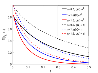
Figure 1: The expectation of $x_{k}-x_{*}$ w.r.t. $\alpha$. $x_{*}$ is the true minimizer. The result is based on the average of 10000 runs.

The SME does not only provide the expectation of the solution, but also provides the fluctuation of the numerical solution $x_{k}$ for any given $\epsilon$. Figure 2 compares the mean and standard deviation (“std”) between $x_{k}$ and $X_{k\epsilon}$ at $\eta=2^{-7}$. The right vertical axis is the value of standard deviation and the two $\operatorname{std}$ curves are very close. In addition, with the same setting, a few hundreds of trajectory samples $x$ are shown together in Figure 3, which illustrate the match both in the mean and in the std between the stochastic ADMM and the SME.

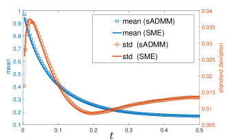
Figure 2: The expectation (left axis) and standard deviation (right axis) of $x_{k}$ (from stochastic ADMM) and $X_{t}$ (from stochastic modified equation) . $\epsilon=2^{-7}$. The results are based on the average of $10000$ independent runs. The over-relaxation parameter $\alpha=1.5$ is used.

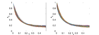
Figure 3: The $400$ sample trajectories from stochastic ADMM (left) and SME (right).

To verify our theorem on the convergence order, a test function $\varphi(x)=x+x^{2}$ is used for the test of the weak convergence error:

$$err:=\max_{1\leq k\leq\lfloor T/\epsilon\rfloor}\left|\operatorname{\mathbb{E}}\varphi(x_{k})-\operatorname{\mathbb{E}}\varphi(X_{k\epsilon})\right|.$$

For each $m=4,5,\ldots,11$, set $\rho=2^{m}/T$, so $\epsilon=T2^{-m}$ and $k=1,2\ldots,2^{m}$. Figure 4 shows the error $err_{m}$ versus $m$ in the semi-log plot for three values of relaxation parameter $\alpha$. The first order convergence rate $err_{m}\propto\epsilon$ is verified.

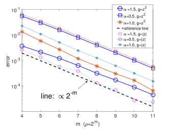
Figure 4: (Verification of the first order approximation )The weak convergence error $err_{m}$ versus $m$ for various $\alpha$ and $\ell_{2}$, $\ell_{1}$ regularization $g$. The step size $\epsilon=1/\rho=2^{-m}T$. $T=0.5$. The result is based on the average of $10^{5}$ independent runs.

We also numerically investigated the convergence rate for the non-smooth penalty $g(z)=|z|$, even though this $\ell_{1}$ regularization function does not satisfy our assumptions. The diffusion term $\Sigma(x)$ is still the same as in the $\ell_{2}$ case since $g(z)$ is deterministic. For the corresponding SDE, at least formally, we can write $\frac{1}{\alpha}dX_{t}=-(4x^{3}+4x-1+\mbox{sign}(x))dt+\sqrt{\epsilon}\left|4x^{3}+2x-1\right|dW_{t}$, by using the sign function as $g^{\prime}(z)$. The rigorous meaning needs the concept of stochastic differential inclusion, which is out of the scope of this work. The numerical results in Figure 4 shows that the weak convergence order $1$ is also true for this $\ell_{1}$ case.

Finally, we test the orders for the standard deviation of $x_{k}$ and $z_{k}$. Th consistence of $\operatorname{std}(x_{k})$ with the SME’s $\operatorname{std}(X_{k\epsilon})$ has been shown in Figure 2. The theoretic prediction is that both are at order $\sqrt{\epsilon}$. We plot the sequences of $\epsilon^{-1/2}\operatorname{std}(x_{k})$ and $\epsilon^{-1/2}\operatorname{std}(z_{k})$ for various $\epsilon$. These two quantities should be the same regardless of $\eta$, and only depends on $\alpha$. which is confirmed by Figure 5.

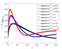
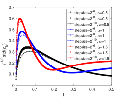
Figure 5: std of $x_{k}$ and $z_{k}$

For the residual, the theoretic prediction is that both $\operatorname{\mathbb{E}}r_{k}$ and $\operatorname{std}r_{k}$ are on the order $\epsilon^{-1}$ if $\alpha\neq 1$. We plot $\epsilon^{-1}\operatorname{\mathbb{E}}(r_{k})$, $\epsilon^{-1}\operatorname{std}(r_{k})$, against the time $t_{k}=k\epsilon$ in Figure 6 and Figure 8, respectively. For the stochastic ADMM scheme with $\alpha=1$, the numerical test shows that $\operatorname{\mathbb{E}}r_{k}$ and $\operatorname{std}r_{k}$ are on the order $\epsilon^{-2}$.

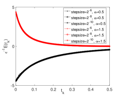
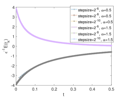
Figure 6: The verification of the mean residual $r_{k}=\mathcal{O}(\epsilon^{-1})$ for $\alpha\neq 1$. $g(z)=z^{2}$ (top) and $g(z)=|z|$(bottom)

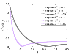
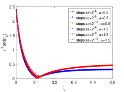
Figure 7: The verification of the std of the residual $r_{k}\sim\epsilon^{-1}$ for $\alpha\neq 1$. $g(z)=z^{2}$ (top) and $g(z)=|z|$(bottom).

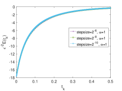
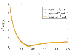
Figure 8: The mean (top) and std (bottom) of the residual $r_{k}\sim\epsilon^{-2}$ for the scheme without relaxation $\alpha=1$. $g(z)=z^{2}$.

Example 2: generalized ridge and lasso regression We perform experiments on the generalized ridge regression.

$$\underset{x\in\mathbb{R}^{d},z\in\mathbb{R}^{m}}{\text{minimize}} \frac{1}{2}\operatorname{\mathbb{E}}_{\boldsymbol{\xi}}\left(\xi_{in}^{\top}x-\xi_{obs}\right)^{2}+g(z)$$ (18)

subject to $$\ Ax-z=0.$$

where $g(z)=\frac{1}{2}\beta\left\|z\right\|^{2}_{2}$ (ridge regression) or $g(z)=\beta\left\|z\right\|_{1}$ (lasso regression), with a constant $\beta>0$. $A$ is a penalty matrix specifying the desired structured pattern of $x$. Among the random $\boldsymbol{\xi}=(\xi_{in},\xi_{obs})\in\mathbb{R}^{n+1}$, $\xi_{in}$ is the zero-mean random (column) vector with uniformly distribution in the hypercube $(-0.5,0.5)^{d}$ with independent components. The labelled data $\xi_{obs}:=\xi_{in}^{\top}v+\zeta$, where $v\in\mathbb{R}^{n}$ is a given vector and $\zeta=\mathcal{N}(0,\sigma_{\zeta}^{2})$ is the zero-mean measurement noise, independent of $\xi_{in}$. The analytic expression of the matrix-valued function $\Sigma(x)$ is available based on the four-order momentums of $\xi_{in}$.

We use a batch size $B$ for the stochastic ADMM ($B=9$ is used in experiments). Then the corresponding SME for the ridge regression problem is

$$\widehat{M}dX_{t}=-\Omega(X_{t}-v)dt-\beta A^{\top}AX_{t}\,dt+\sqrt{\epsilon/B}\Sigma^{1/2}(X_{t})dW_{t}$$

The SME for the lasso regression (formally) is

$$\widehat{M}dX_{t}\in-\Omega(x-v)dt-\frac{1}{2}\beta A^{\top}\mbox{sign}(Ax)dt+\sqrt{\epsilon/B}\Sigma^{1/2}dW_{t}$$

The direct simulation of these stochastic equations has a high computational burden because of the complexity of matrix square root for $\Sigma(x)$. So, our tests are only restricted to the dimension $d=3$.

Set $A$ is the Hilbert matrix multiplied by $0.5$. $\sigma_{\zeta}^{2}=0.1$. $\beta=0.2$. The vector $v$ is set as $\mbox{linspace}(1,2,d)$. The initial $X_{0}=x_{0}$ is the zero vector. $z_{0}=Ax_{0}$.

In algorithms, set $c=1$. We choose the test function $\varphi(x)=\sum_{i=1}^{d}x_{(i)}$. Denote $\varphi_{k}=\varphi(x_{k})$ where $x_{k}$ are the sequence computed from the (unified) stochastic ADMM with the batch size $B$ . Denote $\Phi_{k\epsilon}=\varphi(X_{k\epsilon})$ where $X_{t}$ is the solution of the SME.

Let $\alpha=1.5$, $\omega=1$, $\omega_{1}=1$. $T=40$. We first show in Figure 9 the mean of $\phi_{k}$ and $\Phi_{k\epsilon}$ versus the time $t_{k}=k\epsilon$, for a fixed $\eta=2^{8}$. To test the match of the fluctuation, we plot in Figure 10 the sequence $\epsilon^{-1/2}\operatorname{std}(\varphi_{k})$ and $\epsilon^{-1/2}\operatorname{std}(\Phi_{k})$ for three different values of $\epsilon=2^{-m}T$ with $m=6,7,8$.

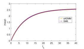
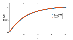
Figure 9: The mean of $\varphi(x_{k})$ from sADMM and $\varphi(X_{k\epsilon})$ from the SME. top: $g(z)=\frac{1}{2}\beta\left\|z\right\|^{2}_{2}$. bottom: $g(z)=\beta\left\|z\right\|_{1}$. The results are based on 100 independent runs.

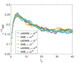
Figure 10: The rescaled std of $\varphi(x_{k})$ from sADMM and $\varphi(X_{k\epsilon})$ from the SME. $g(z)=\frac{1}{2}\beta\left\|z\right\|^{2}_{2}$. The results are based on 400 independent runs.

4 Conclusion

In this paper, we have use the stochastic modified equation(SME) to analyze the dynamics of stochastic ADMM in the large $\rho$ limit (i.e., small step-size $\epsilon$ limit). It is a first order weak approximation to a general family of stochastic ADMM algorithms, including the standard, linearized and gradient-based ADMM with relaxation $\alpha\neq 1$.

Our new continuous-time analysis is the first analysis of stochastic version of ADMM. It faithfully captures the fluctuation of the stochastic ADMM solution and provides a mathematical clear and insightful way to understand the dynamics of stochastic ADMM algorithms.

It is a substantial complementary to the existing ODE-based continuous-time analysis (França et al., 2018; Yuan et al., 2019) for the deterministic ADMM. It is also an important mile-stone for understanding continuous time limit of stochastic algorithms other than stochastic gradient descent (SGD), as we observed new phenonmons like the joint fluctuation of $x$, $z$ and $r$. We provide solid numerical experiments verifying our theory on several examples, including smooth function like quadratic functions and non-smooth function like $\ell_{1}$ norm.

5 Future Work

There are a few natural directions to further explore in future.

First, in the theoretic analysis aspect, for simplicity of analysis, we derive our mathematical proof based on smoothness of $f$ and $g$. As we observed empirically, for non-smooth function like $\ell_{1}$ norm, our continuous-time limit framework would derive a stochastic differential inclusion. A natural follow-up of this work would be develop formal mathematical tools of stochastic differential inclusion to extend our proof to non-smooth functions.

Second, from our stochastic differential equation, we could develop practical rules to choose adaptive step-size $\epsilon$ and batch size by precisely computing the optimal diffusion-fluctuation trade-off to accelerate convergence of stochastic ADMM.

Appendix A Weak Approximation and Stochastic Modified Equations

We introduce and review the concepts for the weak approximation and the stochastic modified equation.

Definition 4 (weak convergence).

We say the family (parametrized by $\epsilon$) of the stochastic sequence $\{x^{\epsilon}_{k}:k\geq 1\}$, $\epsilon>0$, weakly converges to (or is a weak approximation to), a family of continuous-time Ito processes $\{X^{\epsilon}_{t}:t\in\mathbb{R}^{+}\}$ with the order $p$ if they satisfy the following conditions: For any time interval $T>0$ and for any test function $\varphi$ such that $\varphi$ and its partial derivatives up to order $2p+2$ belong to $\mathcal{F}$, there exists a constant $C>0$ and $\epsilon_{0}>0$ such that for any $\epsilon<\epsilon_{0}$,

$$\max_{1\leq k\leq\lfloor T/\epsilon\rfloor}\left|\operatorname{\mathbb{E}}\varphi(X^{\epsilon}_{k\epsilon})-\operatorname{\mathbb{E}}\varphi(x^{\epsilon}_{k})\right|\leq C\epsilon^{p},$$ (19)

The constant $C$ in the above inequality and $\epsilon_{0}$, independent of $\epsilon$, may depend on $T$ and $\varphi$. For the conventional applications to numerical method for SDE (Milstein, 1995), $X^{\epsilon}$ may not depended on $\epsilon$; for the stochastic modified equation in our problem, $X^{\epsilon}$ does depend on $\epsilon$. We drop the subscript $\epsilon$ in $x^{\epsilon}_{k}$ and $X^{\epsilon}_{t}$ for notational ease whenever there is no ambiguity.

The idea of using the weak approximation and the stochastic modified equation was originally proposed by (Li et al., 2017), which is based on an important theorem due to (Milstein, 1986). In brief, this Milstein’s theorem links the one step difference, which has been detailed above, to the global approximation in weak sense, by checking three conditions on the momentums of one step difference. Since we only consider the first order weak approximation, the Milstein’s theorem is introduced in a simplified form below for only $p=1$. The more general situations can be found in Theorem 5 in (Milstein, 1986), Theorem 9.1 in (Milstein, 1995) and Theorem 14.5.2 in (Kloeden & Platen, 2011).

Let the stochastic sequence $\{x_{k}\}$ be recursively defined by the iteration written in the form associated with a function $\mathcal{A}(\cdot,\cdot,\cdot)$:

$$x_{k+1}=x_{k}-\epsilon\mathcal{A}(\epsilon,x_{k},\xi_{k+1}),~{}~{}k\geq 0$$ (20)

where $\{\xi_{k}:k\geq 1\}$ are iid random variables. $x_{0}=x\in\mathbb{R}^{d}$. Define the one step difference $\bar{\Delta}=x_{1}-x$. We use the parenthetical subscript to denote the dimensional components of a vector like $\bar{\Delta}=(\bar{\Delta}_{(i)},1\leq i\leq d)$.

Assume that there exists a function $K_{1}(x)\in\mathcal{F}$ such that $\bar{\Delta}$ satisfies the bounds of the fourth momentum

$$\left|\operatorname{\mathbb{E}}(\bar{\Delta}_{(i)}\bar{\Delta}_{(j)}\bar{\Delta}_{(m)}\bar{\Delta}_{(l)})\right|\leq K_{1}(x)\epsilon^{3}$$ (21)

for any component indices $i,j,m,l\in\{1,2,\ldots,d\}$ and any $x\in\mathbb{R}^{d}$,

For any arbitrary $\epsilon>0$, consider the family of the Ito processes $X^{\epsilon}_{t}$ defined by a stochastic differential equation whose noise depends on the parameter $\epsilon$,

$$dX_{t}=b(X_{t})dt+\sqrt{\epsilon}\sigma(X_{t})dW_{t},$$ (22)

$W_{t}$ is the standard Wiener process in $\mathbb{R}^{d}$. The initial is $X_{0}=x_{0}=x$. The coefficient functions $b$ and $\sigma$ satisfy certain standard conditions; see (Milstein, 1995). Define the one step difference ${\Delta}=X_{\epsilon}-x$ for the SDE (22).

Theorem 5 (Milstein’s weak convergence theorem).

If there exist a constant $K_{0}$ and a function $K_{2}(x)\in\mathcal{F}$ , such that the following conditions of the first three moments on the error $\Delta-\bar{\Delta}$:

$$\left|\operatorname{\mathbb{E}}(X_{\epsilon}-X_{1})\right|\leq K_{0}\epsilon^{2}$$ (23a)

$$\left|\operatorname{\mathbb{E}}(\Delta_{(i)}\Delta_{(j)})-\operatorname{\mathbb{E}}(\bar{\Delta}_{(i)}\bar{\Delta}_{(j)})\right|\leq K_{1}(x)\epsilon^{2}$$ (23b)

$$\left|\operatorname{\mathbb{E}}(\Delta_{(i)}\Delta_{(j)}\Delta_{(l)})-\operatorname{\mathbb{E}}(\bar{\Delta}_{(i)}\bar{\Delta}_{(j)}\bar{\Delta}_{(l)})\right|\leq K_{1}(x)\epsilon^{2}$$ (23c)

hold for any $i,j,l\in\{12,\ldots,d\}$ and any $x\in\mathbb{R}^{d}$, then $\{x_{k}\}$ weakly converges to $\{X_{t}\}$ with the order 1.

In light of the above theorem, we will now call equation (22) the stochastic modified equation (SME) of the iterative scheme (20).

For the SDE (22) at the small noise $\epsilon$, by the Ito-Taylor expansion, it is well-known that $\operatorname{\mathbb{E}}{\Delta}=b(x)\epsilon+\mathcal{O}(\epsilon^{2})$ and $\operatorname{\mathbb{E}}[{\Delta}{\Delta}^{\top}]=\left(b(x)b(x)^{\top}+\sigma(x)\sigma(x)^{\top}\right)\epsilon^{2}+\mathcal{O}(\epsilon^{3})$ and $\operatorname{\mathbb{E}}(\Pi_{m=1}^{s}{\Delta}_{(i_{m})})=\mathcal{O}(\epsilon^{3})$ for all integer $s\geq 3$ and the component index $i_{m}=1,\ldots,d$. Refer to (Kloeden & Platen, 2011) and Lemma 1 in (Li et al., 2017). So, the main receipt to apply the Milstein’s theorem is to examine the conditions of the momentums for the discrete sequence $\bar{\Delta}=x_{1}-x_{0}$.

One prominent work (Li et al., 2017) is to use the SME as a weak approximation to understand the dynamical behaviour of the stochastic gradient descent (SGD). The prominent advantage of this technique is that the fluctuation in the SGD iteration can be well captured by the fluctuation in the SME. Here is the brief result. For the composite minimization problem

$$\min_{x\in\mathbb{R}}f(x)=\operatorname{\mathbb{E}}_{\xi}f(x,\xi),$$

the SGD iteration is $x_{k+1}=x_{k}-\epsilon f^{\prime}(x_{k},\xi_{k+1})$ with the step size $\epsilon$, then by Theorem 5, the corresponding SME of first order approximation is

$$dX_{t}=-f^{\prime}(x)dt+\sqrt{\epsilon}\sigma(x)dW_{t}$$ (24)

with $\sigma(x)=\mbox{std}_{\xi}(f^{\prime}(x,\xi))=(\operatorname{\mathbb{E}}[(f^{\prime}(x)-f^{\prime}(x,\xi))^{2}])^{1/2}$. Details can be found in (Li et al., 2017). The SGD here is analogous to the forward-time Euler-Maruyama approximation since $\mathcal{A}(\epsilon,x,\xi)=f^{\prime}(x,\xi)$.

Appendix B Proof of main theorems

The one step difference is important to consider the weak convergence of the discrete scheme (5). The question is that for one single iteration, from step $k$ to step $k+1$, what is the order of the change of the states $(x,z,u)$. Since For notational ease, we drop the random variable $\xi_{k+1}$ in the scheme (5); the readers bear in mind that $f$ and its derivatives involve $\xi$.

We work on the general ADMM scheme (5). The optimality conditions for the scheme (5) are

$$\omega_{1}\epsilon f^{\prime}(x_{k})+(1-\omega_{1})\epsilon f^{\prime}(x_{k+1})+\epsilon A^{\top}\lambda_{k}$$

$$\qquad+A^{\top}\left(\omega Ax_{k}+(1-\omega)Ax_{k+1}-z_{k}\right)+c(x_{k+1}-x_{k})=0$$ (25a)

$$\epsilon g^{\prime}(z_{k+1})=\epsilon\lambda_{k}+\alpha Ax_{k+1}+(1-\alpha)z_{k}-z_{k+1}$$ (25b)

$$\epsilon\lambda_{k+1}=\epsilon\lambda_{k}+\alpha Ax_{k+1}+(1-\alpha)z_{k}{}-z_{k+1}$$ (25c)

Note that due to (25b) and (25c), the last condition (25c) can be replaced by $\lambda_{k+1}=g^{\prime}(z_{k+1}).$ So, without loss of generality, one can assume that

$$\lambda_{k^{\prime}}\equiv g^{\prime}(z_{k^{\prime}})$$ (26)

for any integer $k^{\prime}\geq 1$. The optimality conditions (25) now can be written only in the variables $(x,z)$:

$$\omega_{1}\epsilon f^{\prime}(x_{k})+(1-\omega_{1})\epsilon f^{\prime}(x_{k+1})+\epsilon A^{\top}g^{\prime}(y_{k})$$

$$\qquad+A^{\top}\left(\omega Ax_{k}+(1-\omega)Ax_{k+1}-z_{k}\right)+c(x_{k+1}-x_{k})=0$$ (27a)

$$\epsilon g^{\prime}(z_{k+1})-\epsilon g^{\prime}(z_{k})=\alpha Ax_{k+1}+(1-\alpha)z_{k}-z_{k+1}$$ (27b)

As $\epsilon\to 0$, we seek the asymptotic expansion of $x_{k+1}-x_{k}$ from (27a) and the asymptotic expansion of $z_{k+1}-z_{k}$ from (27b). The first result is that

$$x_{k+1}-x_{k} =-M^{-1}A^{\top}r_{k}+c_{k}\epsilon,$$ (28a)

$$z_{k+1}-z_{k} =\alpha(I-AM^{-1}A^{\top})r_{k}+c^{\prime}_{k}\epsilon,$$ (28b)

where $r_{k}$ is the residual

$$r_{k}:=Ax_{k}-z_{k}$$ (29)

and the matrix $M$ is

$$M=M_{c,\omega}:=c+(1-\omega)A^{\top}A.$$ (30)

The constant $c_{k}$ and $c^{\prime}_{k}$ are independent of $\epsilon$ but related to $f^{\prime}$, $g^{\prime}$ and other parameters $\alpha,\omega,\omega_{1}$. Throughout the rest of the paper, we shall use the notation $\mathcal{O}(\epsilon^{p})$ to denote the terms $c_{k}\epsilon^{p}$, for $p=1,2,\ldots$. Given any input $(x_{k},z_{k})$, since $r_{k}=Ax_{k}-z_{k}$ may not be zero, then as the step size $\epsilon\to 0$, (28a) and (28a) show that $(x_{k+1},z_{k+1})$ does not converge to $(x_{k},z_{k})$. However we can show that the residual after one step iteration $r_{k+1}$ is always a small number on the order $\mathcal{O}(\epsilon)$, so that the consist condition that as $\epsilon\to 0$, $(x_{k+1},z_{k+1})$ tends to $(x_{k},z_{k})$ holds.

Proposition 6.

We have the following property for the propagation of the residual:

$$r_{k+1}=\left(1-\alpha\right)(I-AM^{-1}A^{\top})r_{k}+\mathcal{O}(\epsilon).$$ (31)

Proof.

By using (27b) and (28b),

$$\begin{split}r_{k+1}&=Ax_{k+1}-z_{k+1}=\left(\frac{1}{\alpha}-1\right)(z_{k+1}-z_{k})+\frac{\epsilon}{\alpha}(g^{\prime}(z_{k+1})-g^{\prime}(z_{k}))\\ &=\left(1-\alpha\right)(I-AM^{-1}A^{\top})r_{k}+\mathcal{O}(\epsilon).\end{split}$$

∎

Remark 4.

If $\alpha=1$, the leading term $\left(1-\alpha\right)(I-AM^{-1}A^{\top})$ vanishes. There are some special cases where the matrix $I-AM^{-1}A^{\top}$ is zero: (1) $A$ is an invertible square matrix and $M=M_{0,1}=A^{\top}A$. (2) $A$ is an orthogonal matrix ($AA^{\top}=A^{\top}A=I$) and the constants satisfy $\omega=c$ such that that $M=I$.

The above proposition is for an arbitrary residual $r_{k}$ as the input in one step iteration. If we choose $r_{0}=0$ at the initial step by setting $z_{0}=Ax_{0}$, then Proposition 6 shows that $r_{1}=Ax_{1}-y_{1}$ become $\mathcal{O}(\epsilon)$ after one iteration. In fact, with assumption $\alpha=1$, we can show $r_{k^{\prime}},\forall k^{\prime}\geq 0$, can be reduced to the order $\epsilon^{2}$ by mathematical induction.

Proposition 7.

If $r_{k}=\mathcal{O}(\epsilon)$, then

$$r_{k+1}=(1-\alpha+\epsilon\alpha g^{\prime\prime}(z_{k}))(r_{k}+A(x_{k+1}-x_{k}))+\mathcal{O}(\epsilon^{3}).$$ (32)

If $\alpha=1$, equation (32) reduces to the second order smallness:

$$r_{k+1}=\epsilon\alpha g^{\prime\prime}(z_{k})(r_{k}+A(x_{k+1}-x_{k}))+\mathcal{O}(\epsilon^{3})=\mathcal{O}(\epsilon^{2}).$$ (33)

Proof.

Since that $r_{k}=Ax_{k}-z_{k}=\mathcal{O}(\epsilon)$, then the one step difference $x_{k+1}-x_{k}$ and $z_{k+1}-z_{k}$ are both at order $\mathcal{O}(\epsilon)$ because of (28a) and (28b). We solve $\delta z:=z_{k+1}-z_{k}$ from (27b) by linearizing the implicit term $g^{\prime}(z_{k+1})$ with the assumption that the third order derivative of $g$ exits:

$$\epsilon g^{\prime\prime}(z_{k})\delta z+\epsilon\mathcal{O}((\delta z)^{2})+\delta z=\alpha(r_{k}+A\delta x).$$

where $\delta x:=x_{k+1}-x_{k}$. Then since $\mathcal{O}((\delta z)^{2})=\mathcal{O}(\epsilon^{2})$, the expansion of $\delta z=z_{k+1}-z_{k}$ in $\epsilon$ is

$$z_{k+1}-z_{k}=\delta z=\alpha(1-\epsilon g^{\prime\prime}(z_{k}))(r_{k}+A\delta x)+\mathcal{O}(\epsilon^{3})$$ (34)

Then

$$\begin{split}r_{k+1}&=r_{k}+A(x_{k+1}-x_{k})-(z_{k+1}-z_{k})\\ &=\Big{(}1-\alpha+\epsilon\alpha g^{\prime\prime}(z_{k})\Big{)}(r_{k}+A(x_{k+1}-x_{k}))+\mathcal{O}(\epsilon^{3})\\ &=(1-\alpha)(r_{k}+(x_{k+1}-x_{k}))+\epsilon\alpha g^{\prime\prime}(z_{k})(r_{k}+A(x_{k+1}-x_{k}))+\mathcal{O}(\epsilon^{3})\end{split}$$

∎

Remark 5.

(32) suggests that $r_{k+1}=(1-\alpha)r_{k}+\mathcal{O}(\epsilon)$. So the condition for the convergence $r_{k}\to 0$ as $k\to\infty$ is $\left|1-\alpha\right|<1$, which matches the range $\alpha\in(0,2)$ used in the relaxation scheme.

Now with the assumption $y_{0}=Ax_{0}$ at initial time, the above analysis shows that $r_{k}$ is $\mathcal{O}(\epsilon)$ and the one step difference $x_{k+1}-x_{k}$ and $z_{k+1}-z_{k}$ are on the order $\mathcal{O}(\epsilon)$ by (28). We shall pursue a more accurate expansion of the one step difference $x_{k+1}-x_{k}$ than (28). Write $f^{\prime}(x_{k+1})=f^{\prime}(x_{k})+f^{\prime\prime}(x_{k})(x_{k+1}-x_{k})+\mathcal{O}((x_{k+1}-x_{k})^{2})$ in equations (27). The asymptotic analysis shows the result below.

Proposition 8.

As $\epsilon\to 0$, the expansion of the one step difference $x_{k+1}-x_{k}$ is

$$\begin{split}M(x_{k+1}-x_{k})&=-A^{\top}r_{k}-\epsilon\left(f^{\prime}(x_{k})+A^{\top}g^{\prime}(y_{k})\right)\\ &+\epsilon^{2}(1-\omega_{1})f^{\prime\prime}(x_{k})M^{-1}\bigg{(}f^{\prime}(x_{k})+A^{\top}g^{\prime}(y_{k})+\frac{1}{\epsilon}A^{\top}r_{k}\bigg{)}+\mathcal{O}(\epsilon^{3}).\end{split}$$ (35)

This expression does not contain the parameter $\alpha$ explicitly, but the residual $r_{k}=Ax_{k}-y_{k}$ significantly depends on $\alpha$ (see Proposition 7). If $\alpha=1$, then $r_{k}$ is on the order of $\epsilon^{2}$, which hints there is no contribution from $r_{k}$ toward the weak approximation of $x_{k}$ at the order 1. But for the relaxation case where $\alpha\neq 1$, $r_{k}$ contains the first order term coming from $z_{k+1}-z_{k}$.

To obtain a second order smallness for some “residual” for the relaxes scheme where $\alpha\neq 1$, we need a new definition, $\alpha$-residual, to account for the gap induced by $\alpha$. Motivated by (25b), we first define

$$r^{\alpha}_{k+1}:=\alpha Ax_{k+1}+(1-\alpha)z_{k}-z_{k+1}.$$ (36)

It is connected to the original residual $r_{k+1}$ and $r_{k}$ since it is easy to check that

$$\begin{split}r^{\alpha}_{k+1}&=\alpha r_{k+1}+(\alpha-1)(z_{k+1}-z_{k})=\alpha r_{k}+\alpha A(x_{k+1}-x_{k})-(z_{k+1}-z_{k})\end{split}$$ (37)

But $r^{\alpha}_{k+1}$ in fact involves information at two successive steps. Obviously, when $\alpha=1$, this $\alpha$-residual $r^{\alpha}$ is the original residual $r=Ax-y$. In our proof, we need a modified $\alpha$-residual, denoted by

$$\widehat{r}^{\alpha}_{k+1}:=\alpha r_{k}+(\alpha-1)(z_{k+1}-z_{k})$$ (38)

We can show that both $r^{\alpha}_{k+1}$ and $\widehat{r}^{\alpha}_{k+1}$ are as small as $\mathcal{O}(\epsilon^{2})$ as $\epsilon$ tends to zero.

Proposition 9.

$r^{\alpha}_{k+1}=\mathcal{O}(\epsilon^{2})$ and $\widehat{r}^{\alpha}_{k+1}=\mathcal{O}(\epsilon^{2})$.

Proof.

In fact, (34) is $z_{k+1}-z_{k}=\alpha(1-\epsilon g^{\prime\prime}(z_{k}))(r_{k}+A(x_{k+1}-x_{k}))+\mathcal{O}(\epsilon^{3})$. By the second equality of (37), (34) becomes $z_{k+1}-z_{k}=(1-\epsilon g^{\prime\prime}(z_{k}))(r^{\alpha}_{k+1}+z_{k+1}-z_{k})+\mathcal{O}(\epsilon^{3})$, i.e.,

$$\begin{split}r^{\alpha}_{k+1}&=\epsilon(1+\epsilon g^{\prime\prime}(z_{k}))g^{\prime\prime}(z_{k})(z_{k+1}-z_{k})+\mathcal{O}(\epsilon^{3})\\ &=\epsilon g^{\prime\prime}(z_{k})(z_{k+1}-z_{k})+\mathcal{O}(\epsilon^{3})\end{split}$$

which is $\mathcal{O}(\epsilon^{2})$ since $z_{k+1}-z_{k}=\mathcal{O}(\epsilon)$.

The difference between $(z_{k+1}-z_{k})$ and $(z_{k+2}-z_{k+1})$, is at the order $\epsilon^{2}$ due to truncation error of the central difference scheme, Then we have the conclusion $\alpha r_{k+1}+(\alpha-1)(z_{k+2}-z_{k+1})$, i.e,

$$\widehat{r}^{\alpha}_{k+1}=\alpha r_{k}+(\alpha-1)(z_{k+1}-z_{k})=\mathcal{O}(\epsilon^{2})$$ (39)

by shifting the subscript $k$ by one.

∎

Corollary 10.

$$r_{k}=\left(\frac{1}{\alpha}-1\right)(z_{k+1}-z_{k})+\mathcal{O}(\epsilon^{2})=\left(\frac{1}{\alpha}-1\right)A(x_{k+1}-x_{k})+\mathcal{O}(\epsilon^{2})$$ (40)

and it follows $z_{k+1}-z_{k}=A(x_{k+1}-x_{k})+\mathcal{O}(\epsilon^{2})$.

Proof.

By (38) and the above proposition, we have $r_{k}=(\frac{1}{\alpha}-1)(z_{k+1}-z_{k})+\mathcal{O}(\epsilon^{2})$. Furthermore, due to (34), $r_{k}=(\frac{1}{\alpha}-1)(z_{k+1}-z_{k})+\mathcal{O}(\epsilon^{2})=(1-{\alpha})(r_{k}+A(x_{k+1}-x_{k}))+\mathcal{O}(\epsilon^{2})$ which gives

$$r_{k}=\left(\frac{1}{\alpha}-1\right)A(x_{k+1}-x_{k})+\mathcal{O}(\epsilon^{2})$$

∎

Proof of Theorem 2.

Combining Proposition 8 and Corollary 10, and noting the Taylor expansion of $g^{\prime}(z_{k})$: $g^{\prime}(y_{k})=g^{\prime}(Ax_{k}-r_{k})=g^{\prime}(Ax_{k})+\mathcal{O}(\epsilon)$ since $r_{k}=\mathcal{O}(\epsilon)$ and putting back random $\xi$ into $f^{\prime}$, we have

$$\begin{split}M(x_{k+1}-x_{k})=&-\epsilon\left(f^{\prime}(x_{k},\xi_{k+1})+A^{\top}g^{\prime}(Ax_{k})\right)\\ &-\left(\frac{1}{\alpha}-1\right)A^{\top}A(x_{k+1}-x_{k})+\mathcal{O}(\epsilon^{2})\end{split}$$ (41)

For convenience, introduce the matrix

$$\widehat{M}:=M+\frac{1-\alpha}{\alpha}A^{\top}A=c+\left(\frac{1}{\alpha}-\omega\right)A^{\top}A.$$ (42)

and let

$$\widehat{x}_{k}:=\widehat{M}x_{k},~{}~{}\text{ and }~{}~{}\delta\widehat{x}_{k+1}=\widehat{M}(x_{k+1}-x_{k})$$

Then

$$\delta\widehat{x}=-\epsilon V^{\prime}(x,\xi)+\epsilon^{2}\left((1-\omega_{1})f^{\prime\prime}M^{-1}V^{\prime}(x)-A^{\top}\theta\right)+\mathcal{O}(\epsilon^{3})$$

The final step is to compute the momentums in the Milstein’s theorem Theorem 5 as follows

1. $$\operatorname{\mathbb{E}}[\delta\widehat{x}]=-\epsilon\operatorname{\mathbb{E}}V^{\prime}(x,\xi)+\mathcal{O}(\epsilon^{2})=-\epsilon V^{\prime}(x)+\mathcal{O}(\epsilon^{2})$$ (43)

2. $$\operatorname{\mathbb{E}}[\delta\widehat{x}\,\delta\widehat{x}^{\top}] =\epsilon^{2}\operatorname{\mathbb{E}}\left(\left[f^{\prime}(x,\xi)+A^{\top}g^{\prime}(x)\right]\left[f^{\prime}(x,\xi)^{\top}+g^{\prime}(x)^{\top}A\right]\right)+\mathcal{O}(\epsilon^{3})$$

   $$=\epsilon^{2}\left(V^{\prime}(x)V^{\prime}(x)^{\top}\right)-\epsilon^{2}\left(f^{\prime}(x)+A^{\top}g^{\prime}(x))(f^{\prime}(x)^{\top}+g^{\prime}(x)^{\top}A)\right)$$

   $$\qquad+\epsilon^{2}\operatorname{\mathbb{E}}\left(\left[f^{\prime}(x,\xi)+A^{\top}g^{\prime}(x)\right]\left[f^{\prime}(x,\xi)^{\top}+g^{\prime}(x)^{\top}A\right]\right)+\mathcal{O}(\epsilon^{3})$$

   $$=\epsilon^{2}\left(V^{\prime}(x)V^{\prime}(x)^{\top}\right)+\epsilon^{2}\operatorname{\mathbb{E}}\left[\left(f^{\prime}(x,\xi)-f^{\prime}(x)\right)\left(f^{\prime}(x,\xi)-f^{\prime}(x)\right)^{\top}\right]+\mathcal{O}(\epsilon^{3})$$

3. It is trivial that $\operatorname{\mathbb{E}}[\Pi_{j=1}^{s}\delta x_{i_{j}}]=\mathcal{O}(\epsilon^{3})$ for $s\geq 3$ and $i_{j}=1,\ldots,d$.

So, Theorem 2 is proved. ∎

Proof of Theorem 1.

Theorem 1 is a special case of Theorem 2. Let $\alpha=1$, $\omega=0$, $c=0$, then $\widehat{M}=A^{\top}A$. ∎

References

Boyd et al. (2011)
Boyd, S., Parikh, N., Chu, E., Peleato, B., Eckstein, J., et al.
Distributed optimization and statistical learning via the alternating
direction method of multipliers.
Foundations and Trends® in Machine learning,
3(1):1–122, 2011.
E et al. (2019)
E, W., Ma, C., and Wu, L.
Machine learning from a continuous viewpoint.
2019.
Eckstein & Bertsekas (1992)
Eckstein, J. and Bertsekas, D. P.
On the Douglas–Rachford splitting method and the proximal point
algorithm for maximal monotone operators.
Mathematical Programming, 55(1-3):293–318, 1992.
França et al. (2018)
França, G., Robinson, D. P., and Vidal, R.
ADMM and accelerated ADMM as continuous dynamical systems.
In Proceedings of the 35th International Conference on Machine
Learning, pp. 1559–1567, 2018.
Freidlin & Wentzell (2012)
Freidlin, M. I. and Wentzell, A. D.
Random Perturbations of Dynamical Systems.
Grundlehren der mathematischen Wissenschaften. Springer-Verlag, New
York, 3 edition, 2012.
Goldfarb et al. (2013)
Goldfarb, D., Ma, S., and Scheinberg, K.
Fast alternating linearization methods for minimizing the sum of two
convex functions.
Mathematical Programming, 141(1-2):349–382, 2013.
Huang et al. (2019)
Huang, F., Chen, S., and Huang, H.
Faster stochastic alternating direction method of multipliers for
nonconvex optimization.
In Chaudhuri, K. and Salakhutdinov, R. (eds.), Proceedings of
the 36th International Conference on Machine Learning, volume 97 of
Proceedings of Machine Learning Research, pp. 2839–2848, Long
Beach, California, USA, 09–15 Jun 2019. PMLR.
URL http://proceedings.mlr.press/v97/huang19a.html.
Kloeden & Platen (2011)
Kloeden, P. and Platen, E.
Numerical Solution of Stochastic Differential Equations.
Stochastic Modelling and Applied Probability. Springer, New York,
corrected edition, 2011.
ISBN 9783662126165.
URL https://books.google.com.hk/books?id=r9r6CAAAQBAJ.
Li et al. (2017)
Li, Q., Tai, C., and E, W.
Stochastic modified equations and adaptive stochastic gradient
algorithms.
In 34th International Conference on Machine Learning, ICML
2017, 34th International Conference on Machine Learning, ICML 2017, pp. 3306–3340. International Machine Learning Society (IMLS), 1 2017.
Li et al. (2019)
Li, Q., Tai, C., and E, W.
Stochastic modified equations and dynamics of stochastic gradient
algorithms I: Mathematical foundations.
Journal of Machine Learning Research, 20(40):1–47, 2019.
Milstein (1995)
Milstein, G.
Numerical Integration of Stochastic Differential Equations,
volume 313 of Mathematics and Its Applications.
Springer, 1995.
ISBN 9780792332138.
URL https://books.google.com.hk/books?id=o2y8Or_a4W0C.
Milstein (1986)
Milstein, G. N.
Weak approximation of solutions of systems of stochastic differential
equations.
Theory of Probability & Its Applications, 30(4):750–766, 1986.
doi: 10.1137/1130095.
URL https://doi.org/10.1137/1130095.
Ouyang et al. (2013)
Ouyang, H., He, N., Tran, L., and Gray, A.
Stochastic alternating direction method of multipliers.
In Dasgupta, S. and McAllester, D. (eds.), Proceedings of the
30th International Conference on Machine Learning, volume 28 of
Proceedings of Machine Learning Research, pp. 80–88, Atlanta,
Georgia, USA, 17–19 Jun 2013. PMLR.
URL http://proceedings.mlr.press/v28/ouyang13.html.
Su et al. (2016)
Su, W., Boyd, S., and Candes, E. J.
A differential equation for modeling Nesterov’s accelerated
gradient method: theory and insights.
Journal of Machine Learning Research, 17(153):1–43, 2016.
Suzuki (2013)
Suzuki, T.
Dual averaging and proximal gradient descent for online alternating
direction multiplier method.
In International Conference on Machine Learning, pp. 392–400, 2013.
Wang & Banerjee (2012)
Wang, H. and Banerjee, A.
Online alternating direction method.
In Proceedings of the 29th International Conference on Machine
Learning, ICML 2012, Proceedings of the 29th International Conference on
Machine Learning, ICML 2012, pp. 1699–1706, 10 2012.
ISBN 9781450312851.
Yuan et al. (2019)
Yuan, H., Zhou, Y., Li, C. J., and Sun, Q.
Differential inclusions for modeling nonsmooth ADMM variants: A
continuous limit theory.
In Chaudhuri, K. and Salakhutdinov, R. (eds.), Proceedings of
the 36th International Conference on Machine Learning, volume 97 of
Proceedings of Machine Learning Research, pp. 7232–7241, Long
Beach, California, USA, 09–15 Jun 2019. PMLR.
URL http://proceedings.mlr.press/v97/yuan19c.html.
Zhong & Kwok (2014)
Zhong, W. and Kwok, J.
Fast stochastic alternating direction method of multipliers.
In International Conference on Machine Learning, pp. 46–54,
2014.
Appendix: Stochastic Modified Equations for Continuous Limit of Stochastic ADMM