[F. Jon Kull, Ph.D.] Dartmouth CollegeHanover, New Hampshire Doctor of Philosophy Computer Science Computer Science Doctor of Philosophy Lorenzo Torresani, Ph.D.Qiang Liu, Ph.D.Bo Zhu, Ph.D.Martin Renqiang Min, Ph.D.

SCALABLE APPROXIMATE INFERENCE AND SOME APPLICATIONS

Abstract

Approximate inference in probability models is a fundamental task in machine learning. Approximate inference provides powerful tools to Bayesian reasoning, decision making, and Bayesian deep learning. The main goal is to estimate the expectation of interested functions w.r.t. a target distribution. When it comes to high dimensional probability models and large datasets, efficient approximate inference becomes critically important.

There are three main traditional frameworks to perform approximate inference. Firstly, adaptive importance sampling methods (IS) draws samples from the adaptively improved importance proposal and correct the bias with importance weights. IS provides an unbiased estimation but is difficult to adaptively optimize the importance proposal because of the large variance from Monte Carlo estimation of the objective. Secondly, Markov chain Monte Carlo (MCMC) runs a long Markov chain to approximate the target. MCMC is theoretically sound and asymptotically consistent but is often slow to converge in practice. Thirdly, variational inference (VI) uses samples from the approximate distribution. VI is practically faster but has been known to lack theoretical consistency guarantees. In this thesis, we propose a new framework for approximate inference, which combines the advantages of these three frameworks and overcomes their limitations. Our proposed four algorithms are motivated by the recent computational progress of Stein’s method. Our proposed algorithms are applied to continuous and discrete distributions under the setting when the gradient information of the target distribution is available or unavailable. Theoretical analysis is provided to prove the convergence of our proposed algorithms. Our adaptive IS algorithm iteratively improves the importance proposal by functionally decreasing the $\mathrm{KL}$ divergence between the updated proposal and the target. When the gradient of the target is unavailable, our proposed sampling algorithm leverages the gradient of a surrogate model and corrects induced bias with importance weights, which significantly outperforms other gradient-free sampling algorithms. In addition, our theoretical results enable us to perform the goodness-of-fit test on discrete distributions.

At the end of the thesis, we propose an importance-weighted method to efficiently aggregate local models in distributed learning with one-shot communication. Results on simulated and real datasets indicate the statistical efficiency and wide applicability of our algorithm.

Declaration

I, Jun Han, confirm that the works presented in this thesis, except as referenced herein, are done by me and have not been submitted in whole or in part for consideration for any other degree or qualification in this, or any other university. Where the information has been derived from other sources, I confirm that this has been indicated in the thesis.

Introduction to Approximate Inference

Background

Probabilistic models provide a powerful framework to capture complex phenomenons and patterns of the data. In discriminative supervised learning, given the input variable ${\boldsymbol{x}}$ and response variable ${\boldsymbol{y}},$ one would define a conditional distribution $p({\boldsymbol{y}}|{\boldsymbol{x}},{\boldsymbol{\theta}}).$ where ${\boldsymbol{\theta}}$ is the parameter of the probability model to be learned. When observations $\mathcal{D}=\{{\boldsymbol{x}}^{i},{\boldsymbol{y}}^{i}\}_{i=1}^{N}$ are available, the task is to learn the parameter ${\boldsymbol{\theta}}$. One popular way to learn ${\boldsymbol{\theta}}$ in discriminative supervised learning is to maximize the log likelihood,

$${\boldsymbol{\theta}}^{*}=\operatorname*{arg\,max}_{{\boldsymbol{\theta}}}\sum_{i=1}^{N}\log p({\boldsymbol{y}}^{i}\mid{\boldsymbol{x}}^{i},{\boldsymbol{\theta}}).$$ (0.1)

Formally, ${\boldsymbol{\theta}}^{*}$ gives the most probable interpretation of the model given the data $\mathcal{D}.$

In Bayesian setting, instead of a deterministic variable ${\boldsymbol{\theta}}$, ${\boldsymbol{\theta}}$ is a random variable. Suppose we have a prior belief distribution on ${\boldsymbol{\theta}}$, $p_{0}({\boldsymbol{\theta}}).$ By Bayesian’s rule, the posterior distribution of ${\boldsymbol{\theta}}$ is

$$p({\boldsymbol{\theta}}\mid\mathcal{D})=\frac{p(\mathcal{D}\mid{\boldsymbol{\theta}})p_{0}({\boldsymbol{\theta}})}{p(\mathcal{D})},$$ (0.2)

where $p(\mathcal{D}\mid{\boldsymbol{\theta}})=\prod_{i}p({\boldsymbol{y}}^{i}\mid{\boldsymbol{x}}^{i},{\boldsymbol{\theta}})$. Here $p(\mathcal{D})$ is the normalization constant,

$$p(\mathcal{D})=\int p(\mathcal{D}\mid{\boldsymbol{\theta}})p_{0}({\boldsymbol{\theta}})d{\boldsymbol{\theta}},$$ (0.3)

which is difficult to compute when the dimension of ${\boldsymbol{\theta}}$ is high and typically intractable in practice. $P(\mathcal{D})$ has wide applications on Bayesian model selections and Bayesian analysis (Murphy, 2012). In this proposal, we will develop an efficient method to effectively estimate $P(\mathcal{D}).$

To predict the response variable ${\boldsymbol{y}}$ on test data ${\boldsymbol{x}}$ from Bayesian perspective, the task is to compute the predictive probability,

$$p({\boldsymbol{y}}\mid{\boldsymbol{x}},\mathcal{D})=\int p({\boldsymbol{y}}\mid{\boldsymbol{x}},{\boldsymbol{\theta}})p({\boldsymbol{\theta}}\mid\mathcal{D})d{\boldsymbol{\theta}},$$ (0.4)

where a challenging integral over ${\boldsymbol{\theta}}$ needs to be solved. In practice, the integration (0.4) is usually intractable. One efficient way is to draw samples $\{{\boldsymbol{\theta}}^{i}\}_{i=1}^{n}$ from $p({\boldsymbol{\theta}}\mid\mathcal{D}),$ and estimate the integration (0.4) using Monte Carlo method,

$$p({\boldsymbol{y}}\mid{\boldsymbol{x}},\mathcal{D})=\frac{1}{n}\sum_{i=1}^{n}p({\boldsymbol{y}}\mid{\boldsymbol{x}},{\boldsymbol{\theta}}^{i}).$$ (0.5)

The key challenging reduces to sample from the posterior distribution $p({\boldsymbol{\theta}}\mid\mathcal{D}).$ The difficulties come from two parts: the distribution of the data is highly complex when the dimension of the data is high; the dataset $\mathcal{D}$ is huge in modern machine learning setting. In the next section, we will introduce two main stream algorithms to tackle such approximate inference problem.

Approximate Inference

In this section, we will introduce two popular algorithms to perform approximate inference, Markov Chain Monte Carlo(MCMC) (Hastings, 1970; Metropolis et al., 1953; Hastings, 1970; Metropolis et al., 1953), and variational inference (Blei et al., 2017). MCMC runs a Markov chain to evolve a set of samples to approximate the target distributions. MCMC is theoretically sound and asymptotically consistent, but is often slow to converge in practice. Variational inference seeks an approximate distributional family and optimizes the approximate distribution whose sample is easy to draw to match the target distribution under some divergence metrics. Variational inference algorithms are practically faster but has been known to lack theoretical consistency guarantees. Finally, we introduce a recently proposed approximate inference algorithm, Stein variational gradient descent (SVGD, Liu & Wang (2016)), which combines advantages of both MCMC and variational inference.

Markov Chain Monte Carlo

Markov chain Monte Carlo (MCMC) methods comprise a class of algorithms for sampling from the distribution of interest. The Metropolis-Hastings (MH) algorithm is the most popular MCMC method Hastings (1970); Metropolis et al. (1953). Let $p({\boldsymbol{\theta}})$ be the target distribution. MH algorithm proposes a transition distribution $q({\boldsymbol{\theta}}^{\prime}|{\boldsymbol{\theta}})$ to sample a candidate value ${\boldsymbol{\theta}}^{\prime}$ given the current value ${\boldsymbol{\theta}}$ according to the transition distribution $q({\boldsymbol{\theta}}^{\prime}|{\boldsymbol{\theta}}).$ At each step, the Markov Chain moves torwards ${\boldsymbol{\theta}}^{\prime}$ with probability

$$\mathcal{A}({\boldsymbol{\theta}},{\boldsymbol{\theta}}^{\prime})=\min(1,\frac{p({\boldsymbol{\theta}}^{\prime})q({\boldsymbol{\theta}}|{\boldsymbol{\theta}}^{\prime})}{p({\boldsymbol{\theta}})q({\boldsymbol{\theta}}^{\prime}|{\boldsymbol{\theta}})}),$$ (0.6)

otherwise it remains to stay at ${\boldsymbol{\theta}}.$

Algorithm 1 Metropolis-Hasting (MH) Algorithm (Hastings, 1970; Metropolis et al., 1953)

  Input: initial distribution $p_{0}({\boldsymbol{\theta}})$ and proposal distribution $q({\boldsymbol{\theta}}^{\prime}|{\boldsymbol{\theta}}).$

  Initialize ${\boldsymbol{\theta}}^{0}$ from $p_{0}({\boldsymbol{\theta}})$.

  for $i=0$ to $M-1$ do

     -sample $u$ from uniform distribution $\mathcal{U}[0,1]$.

     -sample ${\boldsymbol{\theta}}^{\prime}$ from $q({\boldsymbol{\theta}}^{\prime}|{\boldsymbol{\theta}})$.

     -if $u<\mathcal{A}({\boldsymbol{\theta}}^{i},{\boldsymbol{\theta}}^{\prime})=\min(1,\frac{p({\boldsymbol{\theta}}^{\prime})q({\boldsymbol{\theta}}^{i}|{\boldsymbol{\theta}}^{\prime})}{p({\boldsymbol{\theta}}^{i})q({\boldsymbol{\theta}}^{\prime}|{\boldsymbol{\theta}}^{i})}),$ let ${\boldsymbol{\theta}}^{i+1}={\boldsymbol{\theta}}^{\prime}$; else ${\boldsymbol{\theta}}^{i+1}={\boldsymbol{\theta}}^{i}.$

  end for

  Remark: $M$ is number of Markov Chain iteration.

The transition kernel for MH algorithm is

$$K_{\mathrm{MH}}({\boldsymbol{\theta}}^{i+1}|{\boldsymbol{\theta}}^{i})=q({\boldsymbol{\theta}}^{i+1}|{\boldsymbol{\theta}}^{i})\mathcal{A}({\boldsymbol{\theta}}^{i},{\boldsymbol{\theta}}^{\prime})+\delta_{{\boldsymbol{\theta}}^{i}}({\boldsymbol{\theta}}^{i+1})r({\boldsymbol{\theta}}^{i})$$ (0.7)

where $\delta_{x}(y)=1$ iff $x=y$ and $r({\boldsymbol{\theta}}^{i})$ is the term associated with rejection,

$$r({\boldsymbol{\theta}}^{i})=\int_{\mathcal{X}}q({\boldsymbol{\theta}}^{\prime}|{\boldsymbol{\theta}})(1-\mathcal{A}({\boldsymbol{\theta}}^{i},{\boldsymbol{\theta}}^{\prime}))d{\boldsymbol{\theta}}^{\prime}.$$

It is straightforward to verify that $K_{\mathrm{MH}}$ satisfies the detailed balance condition,

$$p({\boldsymbol{\theta}}^{i})K_{\mathrm{MH}}({\boldsymbol{\theta}}^{i+1}|{\boldsymbol{\theta}}^{i})=p({\boldsymbol{\theta}}^{i+1})K_{\mathrm{MH}}({\boldsymbol{\theta}}^{i}|{\boldsymbol{\theta}}^{i+1}),$$

which is the sufficient and necessary condition for the Markov chain to converge to the stationary distribution $p({\boldsymbol{\theta}}).$

Most practical MCMC algorithms, such as Monte Carlo expectation-maximization (MCEM) Wei & Tanner (1990) and Hybrid Monte Carlo Duane et al. (1987); Neal (2012), can be interpreted as special cases or extensions of the MH algorithm.

Hybrid Monte Carlo (HMC) Duane et al. (1987); Neal (2012)

HMC introduces a set of auxiliary ”momentum” $\boldsymbol{v}$ and defines the extended target density

$$p({\boldsymbol{\theta}},\boldsymbol{v})=p({\boldsymbol{\theta}})\mathcal{N}(\boldsymbol{v};\boldsymbol{0},\mathbf{I}),$$ (0.8)

where $\mathcal{N}(\boldsymbol{v};\boldsymbol{0},\mathbf{I})$ is the standard Gaussian distribution. Let $\Delta({\boldsymbol{\theta}})=\partial\log p({\boldsymbol{\theta}})/\partial{\boldsymbol{\theta}}$ and $\epsilon$ be the fixed step size.

Algorithm 2 Hamiltonian Monte Carlo (HMC) Algorithm (Duane et al., 1987; Neal, 2012)

  Input: initial distribution $p_{0}({\boldsymbol{\theta}}).$

  Initialize ${\boldsymbol{\theta}}^{0}$ from $p_{0}({\boldsymbol{\theta}})$

  for $i=0$ to $M-1$ do

     -sample $u$ from uniform distribution $\mathcal{U}[0,1]$ and $\boldsymbol{v}^{\prime}\sim\mathcal{N}(\boldsymbol{v};\boldsymbol{0},\mathbf{I}).$

     -Let ${\boldsymbol{\theta}}_{0}={\boldsymbol{\theta}}^{i}$ and $\boldsymbol{v}_{0}=\boldsymbol{v}^{\prime}+\epsilon\Delta({\boldsymbol{\theta}}_{0}).$

     for $\ell=1,\cdots,L$ do

        -${\boldsymbol{\theta}}_{\ell}={\boldsymbol{\theta}}_{\ell-1}+\epsilon\boldsymbol{v}_{\ell-1}.$

        -$\boldsymbol{v}_{\ell}=\boldsymbol{v}_{\ell-1}+\epsilon_{\ell}\Delta({\boldsymbol{\theta}}_{\ell}),$ where $\epsilon_{\ell}=\epsilon$ for $\ell<L$ and $\epsilon_{L}=\epsilon/2.$

     end for

     -if $u<\mathcal{A}=\min(1,\frac{p({\boldsymbol{\theta}}_{L})}{p({\boldsymbol{\theta}}^{i})})\exp(-\frac{1}{2}(\boldsymbol{v}_{L}^{\top}\boldsymbol{v}_{L})-\boldsymbol{v}^{\prime\top}\boldsymbol{v}^{\prime}),$ then $({\boldsymbol{\theta}}^{i+1},\boldsymbol{v}^{i+1})=({\boldsymbol{\theta}}_{L},\boldsymbol{v}_{L});$

     -else $({\boldsymbol{\theta}}^{i+1},\boldsymbol{v}^{i+1})=({\boldsymbol{\theta}}^{i},\boldsymbol{v}^{\prime}).$

  end for

  Remark: $L$ is the number of leap-frog steps.

When $L=1$ in HMC Algorithm 2, it reduces to well-known Langevin algorithm. Two major drawbacks of MCMC algorithms limit their applications to approximate inference. The first limitation is that it takes a long time for the Markov chains to converge. The second limitation is that it is difficult to measure whether the Markov chains have converged or not. Lastly, widely used MCMC algorithms such as Langevin algorithm and HMC algorithm require the availability of the gradient information of the target distributions, which is impractical in some applications. In some real settings, the gradient of the target distribution is too expensive to calculate or intractable. The major drawbacks of MCMC algorithms motivate us to design better approximate inference algorithms.

Variational Inference

In MCMC methods, our goal is to draw a set of samples $\{{\boldsymbol{\theta}}_{i}\}_{i=1}^{n}$ to approximate $p({\boldsymbol{\theta}}|\mathcal{D})$. Although there is theoretical guarantee that the Markov chains will converge to the target distribution, it is too expensive to draw samples to approximate $p({\boldsymbol{\theta}}|\mathcal{D})$ in some applications. In this case, Wainwright et al. (2008); Blei et al. (2017) use a variational distribution $q({\boldsymbol{\theta}})$ from a distribution family $\mathcal{Q}$, which is easy to sample from, to approximate $p({\boldsymbol{\theta}}|\mathcal{D}).$ To simplify the notation without confusion, we abbreviate $p({\boldsymbol{\theta}}|\mathcal{D})$ as $p({\boldsymbol{\theta}}).$ Before introducing variational methods, let us first introduce the divergence between distributions.

Definition 1.

The $f$-divergence between two probability distributions $q({\boldsymbol{\theta}})$ and $p({\boldsymbol{\theta}})$ is

$$\mathbb{D}_{f}(q({\boldsymbol{\theta}})||p({\boldsymbol{\theta}}))=\mathbb{E}_{q}[f(\frac{p({\boldsymbol{\theta}})}{q({\boldsymbol{\theta}})})-f(1)],$$ (0.9)

where $f:\mathbb{R}_{+}\rightarrow\mathbb{R}$ is any convex function.

Variational inference by $f$-divergence

: As it is intractable to draw samples from the distribution $p({\boldsymbol{\theta}})$ of interest, variational inference uses a simpler distribution $q_{\boldsymbol{\phi}}({\boldsymbol{\theta}})$, parametrized by ${\boldsymbol{\phi}}$, to approximate $p({\boldsymbol{\theta}})$ and draw samples from $q_{\boldsymbol{\phi}}({\boldsymbol{\theta}})$ instead to perform approximate inference. The problem is how to ensure $q_{\boldsymbol{\phi}}({\boldsymbol{\theta}})$ to approximate the distribution $p({\boldsymbol{\theta}})$ of interest. In variational inference, we optimize the parameter ${\boldsymbol{\phi}}$ to

$$\min_{\phi}\mathbb{D}_{f}(q_{{\boldsymbol{\phi}}}({\boldsymbol{\theta}})||p({\boldsymbol{\theta}}))=\min_{\phi}\mathbb{E}_{q}[f(\frac{p({\boldsymbol{\theta}})}{q_{{\boldsymbol{\phi}}}({\boldsymbol{\theta}})})-f(1)].$$ (0.10)

For details, see Blei et al. (2017); Wang et al. (2018).

Choices of function $f$

One nature choice of $f$ is $f(x)=-\log(x).$ We have the $\mathrm{KL}$ divergence between $q_{\boldsymbol{\phi}}({\boldsymbol{\theta}})$ and $p({\boldsymbol{\theta}}),$

$$\min_{\phi}\mathcal{L}(\phi)=\min_{\phi}\mathrm{KL}(q_{{\boldsymbol{\phi}}}({\boldsymbol{\theta}})||p({\boldsymbol{\theta}}))=\min_{\phi}\mathbb{E}_{q}[\log q_{{\boldsymbol{\phi}}}({\boldsymbol{\theta}})-\log p({\boldsymbol{\theta}})].$$ (0.11)

Another widely used choice of $f$ is $f(x)=t^{\alpha}/(\alpha(\alpha-1))$, $\alpha\in\mathbb{R}/\{0,1\},$ which is called $\alpha$-divergence (Hernández-Lobato et al., 2016). Variational inference algorithms typically converge faster than MCMC algorithms. While one major drawback of variational inference algorithms is that it restrict the approximate distribution from the predefined family $\{q_{\phi}({\boldsymbol{\theta}})\},$ which gives poor approximation when the predefined distribution family $\{q_{\phi}({\boldsymbol{\theta}})\}$ deviates from the complex target distribution $p({\boldsymbol{\theta}}).$ In most cases, the expectation (0.11) doesn’t have a closed form, which casts a challenging optimization problem. In practice, to optimize the parameter $\phi$, VI algorithms typically draw a set of samples $\{{\boldsymbol{\theta}}_{i}\}_{i=1}^{n}$ and do Monte Carlo estimation of the objective (0.11),

$$\nabla_{\phi}\mathcal{L}(\phi)\approx\frac{1}{n}\sum_{i=1}^{n}[\nabla_{\phi}\log q_{\phi}({\boldsymbol{\theta}}_{i})(\log p({\boldsymbol{\theta}}_{i})-\log q_{\phi}({\boldsymbol{\theta}}_{i}))].$$ (0.12)

However, the Monte Carlo estimation (0.12) has large variance. We will discuss techniques to reduce the variance of such Monte Carlo estimation.

Black-Box Variational Inference

(BBVI, Ranganath et al. (2014)) In some applications, the gradient of the target distribution $p({\boldsymbol{\theta}})$ w.r.t. ${\boldsymbol{\theta}}$ is unavailable. Based on the fact that $\mathbb{E}_{q_{\phi}({\boldsymbol{\theta}})}[\nabla_{\phi}\log q_{\phi}({\boldsymbol{\theta}})]=0,$ we can construct a simple form of control variates to reduce the variance,

$$\nabla_{\phi}\mathcal{L}(\phi)\approx\frac{1}{n}\sum_{i=1}^{n}[\nabla_{\phi}\log q_{\phi}({\boldsymbol{\theta}}_{i})(\log q_{\phi}({\boldsymbol{\theta}}_{i})-\log p({\boldsymbol{\theta}}_{i}))]+\lambda\frac{1}{n}\sum_{i=1}^{n}\nabla_{\phi}\log q_{\phi}({\boldsymbol{\theta}}_{i})],$$ (0.13)

where $\lambda$ is the coefficient and has the optimal form

$$\lambda=-\mathrm{Var}(\nabla_{\phi}\log q_{\phi}({\boldsymbol{\theta}}))^{-1}\mathrm{Cov}[\nabla_{\phi}\log q_{\phi}({\boldsymbol{\theta}})(\log q_{\phi}({\boldsymbol{\theta}})-\log p({\boldsymbol{\theta}}),\nabla_{\phi}\log q_{\phi}({\boldsymbol{\theta}})],$$ (0.14)

and the variance, covariance matrix can be estimated empirically. In some cases, (0.13) still has relatively large variance. In order to have a smaller variance, large sample size $\{{\boldsymbol{\theta}}_{i}\}_{i=1}^{n}$ is required, which might be impractical when the evaluation of the target distribution $\log p({\boldsymbol{\theta}})$ is expensive. At the end of the thesis, we will adopt a more efficient method to reduce the variance.

Discussions on implicit and semi-implicit choice of $q_{\boldsymbol{\phi}}({\boldsymbol{\theta}})$

To remove the restriction of choosing the surrogate distribution $q_{\phi}({\boldsymbol{\theta}})$ from the predefined family $\{q_{\phi}({\boldsymbol{\theta}})\},$ the implicit choice and semi-implicit choice of the distribution $\{q_{\phi}({\boldsymbol{\theta}})\}$ have recently been proposed (Wang & Liu, 2016; Mescheder et al., 2017; Tran et al., 2017; Yin & Zhou, 2018). Basically, they construct a powerful variable transform parametrized by a deep neural network as follows,

$${\boldsymbol{\theta}}=f_{\phi}(\epsilon),~{}q_{\boldsymbol{\phi}}({\boldsymbol{\theta}})=q_{0}(f_{\phi}^{-1}({\boldsymbol{\theta}}))|\frac{\partial f_{\phi}^{-1}({\boldsymbol{\theta}})}{\partial{\boldsymbol{\theta}}}|,~{}\mathrm{where}~{}\epsilon\sim q_{0}(\epsilon),$$ (0.15)

and optimizes a certain divergence between the transformed distribution $q_{\boldsymbol{\phi}}({\boldsymbol{\theta}})$ and the target distribution $p({\boldsymbol{\theta}}).$ As long as the transform is expressive enough, the transformed distribution $q_{\boldsymbol{\phi}}({\boldsymbol{\theta}})$ can arbitrarily approximate the target distribution $p({\boldsymbol{\theta}}).$ Implicit probability can be applied to applications when the samples from $q_{\boldsymbol{\phi}}({\boldsymbol{\theta}})$ is needed. However, as shown in (0.32), it is challenging to calculate the density realization of $q_{\boldsymbol{\phi}}({\boldsymbol{\theta}})$ as the inverse of $f_{\phi}$ is typically unavailable and cumbersome to compute the determinant of the Jacobian matrix $\frac{\partial f_{\phi}^{-1}({\boldsymbol{\theta}})}{\partial{\boldsymbol{\theta}}}$, which limits its application. Most importantly, it is also difficult to stably train such a transform using standard optimization methods, which is the main reason limiting its real applications. Semi-implicit $q_{\boldsymbol{\phi}}({\boldsymbol{\theta}})$ (Yin & Zhou, 2018) has been proposed to alleviate the problem in implicit model $q_{\boldsymbol{\phi}}({\boldsymbol{\theta}})$. But the unstable problem still exists.

Stein Variational Gradient Descent

Stein variational gradient descent (SVGD) (Liu & Wang, 2016) is a nonparametric variational inference algorithm that iteratively transports a set of particles to approximate a given target distribution by performing a type of functional gradient descent on the KL divergence. We give a quick overview of its main idea in this section. To make notations easy to read, we use the notation $p({\boldsymbol{x}})$ to be the target distribution instead of $p({\boldsymbol{\theta}})$ in the following.

Preliminary Notations

Before introducing SVGD, let us define some notations, which will be used in the whole thesis. We always assume ${\boldsymbol{x}}=[x_{1},\cdots,x_{d}]^{\top}\in\mathbb{R}^{d}$. Given a positive definite kernel $k({\boldsymbol{x}},{\boldsymbol{x}}^{\prime})$, there exists an unique reproducing kernel Hilbert space (RKHS) $\mathcal{H}_{0}$, formed by the closure of functions of form $f({\boldsymbol{x}})=\sum_{i}a_{i}k({\boldsymbol{x}},{\boldsymbol{x}}_{i})$ where $a_{i}\in\mathbb{R}$, equipped with inner product $\langle f,~{}g\rangle_{\mathcal{H}_{0}}=\sum_{ij}a_{i}k({\boldsymbol{x}}_{i},{\boldsymbol{x}}_{j})b_{j}$ for $g({\boldsymbol{x}})=\sum_{j}b_{j}k({\boldsymbol{x}},{\boldsymbol{x}}_{j})$. Denote by $\mathcal{H}=\mathcal{H}_{0}^{d}=\mathcal{H}_{0}\times\cdots\times\mathcal{H}_{0}$ the vector-valued function space formed by $\boldsymbol{f}=[f_{1},\ldots,f_{d}]^{\top}$, where $f_{i}\in\mathcal{H}_{0}$, $i=1,\ldots,d$, equipped with inner product $\langle\boldsymbol{f},~{}\boldsymbol{g}\rangle_{\mathcal{H}}=\sum_{l=1}^{d}\langle f_{l},~{}g_{l}\rangle_{\mathcal{H}_{0}},$ for $\boldsymbol{g}=[g_{1},\ldots,g_{d}]^{\top}.$ Equivalently, $\mathcal{H}$ is the closure of functions of form $\boldsymbol{f}({\boldsymbol{x}})=\sum_{i}\boldsymbol{a}_{i}k({\boldsymbol{x}},{\boldsymbol{x}}_{i})$ where $\boldsymbol{a}_{i}\in\mathbb{R}^{d}$ with inner product $\langle\boldsymbol{f},~{}\boldsymbol{g}\rangle_{\mathcal{H}}=\sum_{ij}\boldsymbol{a}_{i}^{\top}\boldsymbol{b}_{j}k({\boldsymbol{x}}_{i},{\boldsymbol{x}}_{j})$ for $\boldsymbol{g}({\boldsymbol{x}})=\sum_{i}\boldsymbol{b}_{i}k({\boldsymbol{x}},{\boldsymbol{x}}_{i})$. See e.g., Berlinet & Thomas-Agnan (2011) for more background on RKHS.

Let $p({\boldsymbol{x}})$ be a continuous-valued positive density function on $\mathbb{R}^{d}$ which we want to approximate with a set of particles $\{{\boldsymbol{x}}_{i}\}_{i=1}^{n}$. SVGD starts with a set of initial particles $\{{\boldsymbol{x}}_{i}\}_{i=1}^{n}$, and updates the particles iteratively by

$${\boldsymbol{x}}_{i}\leftarrow{\boldsymbol{x}}_{i}+\epsilon{\boldsymbol{\phi}}({\boldsymbol{x}}_{i}),~{}~{}~{}~{}\forall i=1,\ldots,n,$$ (0.16)

where $\epsilon$ is a step size, and ${\boldsymbol{\phi}}\colon\mathbb{R}^{d}\to\mathbb{R}^{d}$ is a velocity field which should be chosen to drive the particle distribution closer to the target. Assume the distribution of the particles at the current iteration is $q$, and $q_{[\epsilon{\boldsymbol{\phi}}]}$ is the distribution of the updated particles ${\boldsymbol{x}}^{\prime}={\boldsymbol{x}}+\epsilon{\boldsymbol{\phi}}({\boldsymbol{x}})$. The optimal choice of ${\boldsymbol{\phi}}$ can be framed into the following optimization problem:

$${\boldsymbol{\phi}}^{*}=\operatorname*{arg\,max}_{{\boldsymbol{\phi}}\in\mathcal{F}}\bigg{\{}-\frac{d}{d\epsilon}\mathrm{KL}(q_{[\epsilon{\boldsymbol{\phi}}]}~{}||~{}p)\big{|}_{\epsilon=0}\bigg{\}},$$ (0.17)

where $\mathcal{F}$ is the set of candidate velocity fields, and ${\boldsymbol{\phi}}$ is chosen in $\mathcal{F}$ to maximize the decreasing rate on the KL divergence between the particle distribution and the target.

In SVGD, $\mathcal{F}$ is chosen to be the unit ball of a vector-valued reproducing kernel Hilbert space (RKHS) $\mathcal{H}=\mathcal{H}_{0}\times\cdots\times\mathcal{H}_{0}$, where $\mathcal{H}_{0}$ is a RKHS formed by scalar-valued functions associated with a positive definite kernel $k({\boldsymbol{x}},{\boldsymbol{x}}^{\prime})$, that is, $\mathcal{F}=\{{\boldsymbol{\phi}}\in\mathcal{H}\colon||{\boldsymbol{\phi}}||_{\mathcal{H}}\leq 1\}.$ This choice of $\mathcal{F}$ allows us to consider velocity fields in infinite dimensional function spaces while still obtaining computationally tractable solution.

A key step towards solving (0.17) is to observe that the objective function in (0.17) is a simple linear functional of ${\boldsymbol{\phi}}$ that connects to Stein operator (Oates et al., 2017; Gorham & Mackey, 2015; Liu & Wang, 2016; Gorham & Mackey, 2017; Chen et al., 2018),

$$~{}-\frac{d}{d\epsilon}\mathrm{KL}(q_{[\epsilon{\boldsymbol{\phi}}]}~{}||~{}p)\big{|}_{\epsilon=0}=\mathbb{E}_{x\sim q}[{\mathcal{A}^{\top}_{p}}{\boldsymbol{\phi}}({\boldsymbol{x}})],$$ (0.18)

$$\!\!\!\!\!\!\!\text{with}~{}~{}~{}{\mathcal{A}^{\top}_{p}}{\boldsymbol{\phi}}({\boldsymbol{x}})=\nabla_{\boldsymbol{x}}\log p({\boldsymbol{x}})^{\top}{\boldsymbol{\phi}}({\boldsymbol{x}})+\nabla_{{\boldsymbol{x}}}^{\top}{\boldsymbol{\phi}}({\boldsymbol{x}}),$$ (0.19)

where ${\mathcal{A}_{p}}$ is a linear operator called Stein operator and is formally viewed as a column vector similar to the gradient operator $\nabla_{{\boldsymbol{x}}}$. The Stein operator ${\mathcal{A}_{p}}$ is connected to Stein’s identity which shows that the RHS of (0.106) is zero if $p=q$:

$$\mathbb{E}_{{\boldsymbol{x}}\sim p}[{\mathcal{A}^{\top}_{p}}{\boldsymbol{\phi}}({\boldsymbol{x}})]=0.$$ (0.20)

This corresponds to $\frac{d}{d\epsilon}\mathrm{KL}(q_{[\epsilon{\boldsymbol{\phi}}]}~{}||~{}p)\big{|}_{\epsilon=0}=0$ since there is no way to further decease the KL divergence when $p=q$. Eq. (0.20) is a simple result of integration by parts assuming the value of $p({\boldsymbol{x}}){\boldsymbol{\phi}}({\boldsymbol{x}})$ vanishes on the boundary of the integration domain.

Therefore, the optimization in (0.17) reduces to

$$\!\!\!\!\mathcal{D}_{\mathcal{F}}(q||p)\overset{def}{=}\max_{{\boldsymbol{\phi}}\in\mathcal{F}}\left\{\mathbb{E}_{{\boldsymbol{x}}\sim q}\left[{\mathcal{A}^{\top}_{p}}{\boldsymbol{\phi}}({\boldsymbol{x}})\right]\right\},$$ (0.21)

where $\mathbb{D}_{\mathcal{F}}(q~{}||~{}p)$ is the kernelized Stein discrepancy (KSD) defined in Liu et al. (2016); Chwialkowski et al. (2016).

Observing that (0.21) is “simple” in that it is a linear functional optimization on a unit ball of a Hilbert space, Liu & Wang (2016) showed that (0.17) has a simple closed-form solution:

$${\boldsymbol{\phi}}^{*}({\boldsymbol{x}}^{\prime})\propto\mathbb{E}_{{\boldsymbol{x}}\sim q}[{\mathcal{A}_{p}}k({\boldsymbol{x}},{\boldsymbol{x}}^{\prime})],$$ (0.22)

where ${\mathcal{A}_{p}}$ is applied to variable ${\boldsymbol{x}}$, and

$$\mathbb{D}^{2}_{\mathcal{F}}(q\mid\mid p)=\mathbb{E}_{{\boldsymbol{x}},{\boldsymbol{x}}^{\prime}\sim q}[\kappa_{p}(\boldsymbol{x},\boldsymbol{x}^{\prime})],$$ (0.23)

where $\kappa_{p}(\boldsymbol{x},\boldsymbol{x}^{\prime}):=({\mathcal{A}}_{p}^{\prime})^{\top}({\mathcal{A}_{p}}k({\boldsymbol{x}},{\boldsymbol{x}}^{\prime}))$ and ${\mathcal{A}^{\prime}_{p}}$ denotes the Stein operator applied on variable ${\boldsymbol{x}}^{\prime}$. Here $\kappa_{p}(\boldsymbol{x},\boldsymbol{x}^{\prime})$ can be calculated explicitly in Theorem 3.6 of Liu et al. (2016),

$$\kappa_{p}(\boldsymbol{x},\boldsymbol{y})= \boldsymbol{s}_{p}(\boldsymbol{x})^{\top}k(\boldsymbol{x},\boldsymbol{y})\boldsymbol{s}_{p}(\boldsymbol{y})+\boldsymbol{s}_{p}(\boldsymbol{x})^{\top}\nabla_{\boldsymbol{y}}k(\boldsymbol{x},\boldsymbol{y})$$ (0.24)

$$+\boldsymbol{s}_{p}(\boldsymbol{y})^{\top}\nabla_{\boldsymbol{x}}k(\boldsymbol{x},\boldsymbol{y})+\nabla_{\boldsymbol{x}}\cdot(\nabla_{\boldsymbol{y}}k(\boldsymbol{x},\boldsymbol{y})).$$

The Stein variational gradient direction ${\boldsymbol{\phi}}^{*}$ provides a theoretically optimal direction that drives the particles towards the target $p({\boldsymbol{x}})$ as fast as possible. In practice, SVGD approximates $q({\boldsymbol{x}})$ using a set of particles, $\{{\boldsymbol{x}}_{i}\}_{i=1}^{n}$ iteratively updated by

$$\!\!{\boldsymbol{x}}_{i}\leftarrow{\boldsymbol{x}}_{i}+\frac{\epsilon}{n}\Delta{\boldsymbol{x}}_{i},\text{~{}where~{}}\Delta{\boldsymbol{x}}_{i}=\sum_{j=1}^{n}[\nabla\log p({\boldsymbol{x}}_{j})k({\boldsymbol{x}}_{j},{\boldsymbol{x}}_{i})+\nabla_{{\boldsymbol{x}}_{j}}k({\boldsymbol{x}}_{j},{\boldsymbol{x}}_{i})],$$ (0.25)

where $k({\boldsymbol{x}},{\boldsymbol{x}}^{\prime})$ is any positive definite kernel; the term with the gradient $\nabla\log p({\boldsymbol{x}})$ drives the particles to the high probability regions of $p({\boldsymbol{x}})$, and the term with $\nabla k({\boldsymbol{x}},{\boldsymbol{x}}^{\prime})$ acts as a repulsive force to keep the particles away from each other to quantify the uncertainty.

Thesis Outline and Contributions

In this section, we will first provide the outline flow and dependence of different chapters in the thesis. Then we will briefly summarize the contributions of our thesis in each chapter.

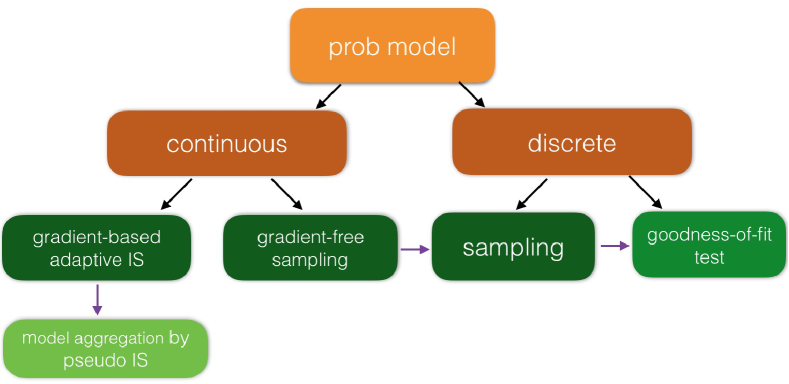
Figure 1: The flow and dependence of the thesis. A gradient-based adaptive importance sampling on continuous-valued distribution is proposed in Chapter Adaptive Importance Sampling. A gradient-free sampling on continuous-valued distribution is proposed in Chapter Gradient-Free Sampling on Continuous Distributions. A sampling algorithm on discrete-valued distribution is proposed in Chapter Sampling from Discrete Distributions, which is motivated from gradient-free sampling method. A goodness-of-fit test algorithm is proposed in Chapter Goodness-of-fit testing on Discrete Distributions, which is motivated by results of Chapter Sampling from Discrete Distributions. Distributed model aggregation algorithm by pseudo importance sampling is proposed in Chapter Distributed Model Aggregation by Pseudo Importance Sampling, which is closely related to the importance sampling trick used in Chapter Adaptive Importance Sampling.

Thesis Flow and Dependence

Firstly, we propose a gradient-based adaptive importance sampling on continuous-valued distribution in Chapter Adaptive Importance Sampling. Secondly, we propose a gradient-free sampling on continuous-valued distribution in Chapter Gradient-Free Sampling on Continuous Distributions. Thirdly, we propose a sampling algorithm on discrete-valued distribution in Chapter Sampling from Discrete Distributions, which is motivated from gradient-free sampling method. Fourthly, based on results of Chapter Sampling from Discrete Distributions, we propose a goodness-of-fit test algorithm in Chapter Goodness-of-fit testing on Discrete Distributions. Finally, we propose importance-weighted method to distributed model aggregation, which is motivated by a form of by importance sampling and is termed as pseudo importance sampling in Chapter Distributed Model Aggregation by Pseudo Importance Sampling.

Thesis Contributions

The contributions of the thesis can be summarized in three main parts. Firstly, we propose three new approximate inference algorithms which can be applied to continuous-valued distributions. Secondly, we propose one sampling algorithm on discrete-valued distributions and one goodness-of-fit testing algorithm, which test whether a set of data $\{{\boldsymbol{z}}_{i}\}_{i=1}^{n}$ is the candidate distribution, on discrete-valued distributions. Finally, we present one effective method, which is motivated from the widely-used tool in approximate inference, to efficiently aggregate distributed models in the one-shot communication setting. Theoretical analysis is provided to analyze the convergence or other properties of our algorithms. Extensive experiments are conducted to demonstrate the effectiveness and wide applicability of all our proposed algorithms.

In the following, we first emphasize our contributions of approximate inference algorithms on continuous-valued distributions. Specifically, we propose a nonparametric adaptive importance sampling algorithm by decoupling the iteratively updated particles of SVGD $\{{\boldsymbol{x}}_{i}^{\ell}\}_{i=1}^{n}$ into two sets: leader particles ${\boldsymbol{x}}_{A}^{\ell}=\{{\boldsymbol{x}}_{i}^{\ell}\colon i\in A\}$ and follower particles ${\boldsymbol{x}}_{B}^{\ell}=\{{\boldsymbol{x}}_{i}^{\ell}\colon i\in B\}$, with $B=\{1,\ldots,n\}\setminus A$. The leader particles is applied to construct the transform and the follower particles are updated by the constructed transform, $\boldsymbol{x}_{i}^{\ell+1}\leftarrow\boldsymbol{x}_{i}^{\ell}+\epsilon{\boldsymbol{\phi}}_{\ell+1}(\boldsymbol{x}_{i}^{\ell}),~{}\forall i\in A\cup B,$ where ${\boldsymbol{\phi}}_{\ell+1}(\cdot)$ is constructed by only using particles in set $A,$

$$\!\!\!\!\!\!\!\!{\boldsymbol{\phi}}_{\ell+1}(\cdot)=\frac{1}{|A|}\sum_{j\in A}[\nabla\log p(\boldsymbol{x}_{j}^{\ell})k(\boldsymbol{x}_{j}^{\ell},\cdot)+\nabla_{\boldsymbol{x}_{j}^{\ell}}k(\boldsymbol{x}_{j}^{\ell},\cdot)].$$

With such a transform, the distribution of the updated particles in ${\boldsymbol{x}}_{B}$ satisfies

$$q_{\ell}=({\boldsymbol{T}}_{\ell}\circ\cdots\circ{\boldsymbol{T}}_{1})\sharp q_{0},\quad\ell=1,\ldots,K,$$ (0.26)

where the importance proposal $q_{\ell}$ forms increasingly better approximation of the target $p$ as $\ell$ increases. Conditional on ${\boldsymbol{x}}_{A}^{\ell},$ particles in ${\boldsymbol{x}}_{B}^{\ell}$ are i.i.d. and hence can provide an unbiased estimation of the integral $\mathbb{E}_{{\boldsymbol{x}}\sim q_{\ell}}[\frac{p({\boldsymbol{x}})}{q_{\ell}({\boldsymbol{x}})}h({\boldsymbol{x}})]$ for any function $h({\boldsymbol{x}}).$ Our importance proposal is not restricted to the predefined distributional family as traditional adaptive importance sampling methods do. The $\mathrm{KL}$ divergence between the updated proposal $q_{\ell}$ and the target distribution is also maximally decreased in a functional space, which inherits from the theory of SVGD (Liu, 2017). We apply our proposed algorithm to evaluate the normalization constant of various probability models including restricted Boltzmann machine and deep generative model to demonstrate the effectiveness of our proposed algorithm, where the original SVGD cannot be applied in such tasks. We propose a novel sampling algorithm for continuous-valued target distribution when the gradient information of the target distribution is unavailable. iteratively updated by ${\boldsymbol{x}}_{i}\leftarrow{\boldsymbol{x}}_{i}+\frac{\epsilon}{n}\Delta{\boldsymbol{x}}_{i}$, where

$$\Delta{\boldsymbol{x}}_{i}\propto\sum_{j=1}^{n}\!w({\boldsymbol{x}}_{j})\big{[}\nabla\log\rho({\boldsymbol{x}}_{j})k({\boldsymbol{x}}_{j},{\boldsymbol{x}}_{i})+\nabla_{{\boldsymbol{x}}_{j}}k({\boldsymbol{x}}_{j},{\boldsymbol{x}}_{i})\big{]},$$ (0.27)

which replaces the true gradient $\nabla\log p({\boldsymbol{x}})$ with a surrogate gradient $\nabla\log\rho({\boldsymbol{x}})$ of an arbitrary auxiliary distribution $\rho({\boldsymbol{x}})$, and then uses an importance weight $w({\boldsymbol{x}}_{j}):=\rho({\boldsymbol{x}}_{j})/p({\boldsymbol{x}}_{j})$ to correct the bias introduced by the surrogate $\rho({\boldsymbol{x}})$. Perhaps surprisingly, we show that the new update can be derived as a standard SVGD update by using an importance weighted kernel $w({\boldsymbol{x}})w({\boldsymbol{x}}^{\prime})k({\boldsymbol{x}},{\boldsymbol{x}}^{\prime})$, and hence immediately inherits the theoretical proprieties of SVGD; for example, particles updated by (0.143) can be viewed as a gradient flow of KL divergence similar to the original SVGD (Liu, 2017). Empirical experiments demonstrate that our proposed gradient-free SVGD significantly outperforms gradient-free Markov Chain Monte Carlo sampling baselines on various probability models with intractable normalization constant and unavailable gradient information of the target distribution.

We propose a gradient-free black-box importance sampling algorithm, which equips any given set of particles $\{{\boldsymbol{x}}_{i}\}_{i=1}^{n}$ with a set of importance weights $\{u_{i}\}_{i=1}^{n}$ such that

$$\sum_{i=1}^{n}u_{i}h(\boldsymbol{x}_{i})\approx\mathbb{E}_{{\boldsymbol{x}}\sim p}[h(\boldsymbol{x})],$$ (0.28)

for general test function $h(\boldsymbol{x}).$ To achieve this goal, we will leverage our result from gradient-free KSD defined as follows,

$$\widetilde{\mathbb{S}}(q,p)=\mathbb{E}_{\boldsymbol{x},\boldsymbol{y}\sim q}[w(\boldsymbol{x})\kappa_{\rho}(\boldsymbol{x},\boldsymbol{y})w(\boldsymbol{y})]\geq 0,$$ (0.29)

where $\kappa_{\rho}(\boldsymbol{x},\boldsymbol{y})$ can be evaluated by the formula (0.24) and does not require the gradient of the target distribution $p({\boldsymbol{x}}).$ (0.29) provides a metric to measure the closeness between $q({\boldsymbol{x}})$ and $p({\boldsymbol{x}})$ when the samples $\{{\boldsymbol{x}}_{i}\}_{i=1}^{n}$ and the evaluation of the target $p({\boldsymbol{x}})$ are available. Motivated from (Liu & Lee, 2017), we propose a gradient-free black-box importance sampling algorithm by optimizing a set of importance weights $\{u_{i}\}_{i=1}^{n}$ for any given set of particles $\{{\boldsymbol{x}}_{i}\}_{i=1}^{n}$ through the following quadratic optmization

$$\begin{split}\hat{\boldsymbol{u}}=\operatorname*{arg\,min}_{\boldsymbol{u}}\bigg{\{}\boldsymbol{u}^{\top}\widetilde{\boldsymbol{K}}_{p}\boldsymbol{u},~{}~{}s.t.~{}~{}\sum_{i=1}^{n}u_{i}=1,~{}~{}~{}u_{i}\geq 0\bigg{\}},\end{split}$$ (0.30)

where $\widetilde{\boldsymbol{K}}_{p}=\{w({\boldsymbol{x}}_{i})\kappa_{\rho}(\boldsymbol{x}_{i},\boldsymbol{x}_{j})w({\boldsymbol{x}}_{j})\}_{i,j=1}^{n}$ and $\boldsymbol{u}=\{u_{i}\}_{i=1}^{n}.$ For more details of the idea and the approximation error, please refer to Chapter Gradient-Free Sampling on Continuous Distributions.

In the second part of the thesis, we propose two approximate inference algorithms on discrete-valued distributions. We propose a new algorithm to sample from the discrete-valued distributions. Our proposed algorithm is based on the fact that the discrete-valued distributions can be bijectively mapped to the piecewise continuous-valued distributions. Since the piecewise continuous-valued distributions are non-differentiable, gradient-based sampling algorithms cannot be applied in this setting. Our proposed sample-efficient GF-SVGD is a natural choice. To construct effective surrogate distributions $\rho({\boldsymbol{x}})$ in GF-SVGD, we propose a simple transformation, the inverse of dimension-wise Gaussian c.d.f. $F({\boldsymbol{x}})$ (its p.d.f. $p_{0}({\boldsymbol{x}})$, $F^{\prime}({\boldsymbol{x}})=p_{0}({\boldsymbol{x}})$), to transform the piecewise continuous-valued distributions to a simple form of continuous distributions. With such a straightforward transform, the effective surrogate distribution $\rho({\boldsymbol{x}})$ in GF-SVGD is natural to construct. The detail of our sampling algorithm is provided in Chapter Sampling from Discrete Distributions. Empirical experiments on large-scale discrete graphical models demonstrate the effectiveness of our proposed algorithm.

As a direct application, we propose a principled ensemble method to train the binarized neural networks (BNN). We train an ensemble of $n$ neural networks (NN) with the same architecture ($n\geq 2$). Let $\boldsymbol{W}_{i}^{b}$ be the binary weight of model $i$, for $i=1,\cdots,n$, and $p_{*}(\boldsymbol{W}_{i}^{b};D)$ be the target probability model with softmax layer as last layer given the data $D$. Learning the target probability model is framed as drawing $n$ samples $\{\boldsymbol{W}_{i}^{b}\}_{i=1}^{n}$ to approximate the posterior distribution $p_{*}(\boldsymbol{W}^{b};D)$. We apply multi-dimensional transform $F$ to transform the original discrete-valued target to the target distribution of real-valued $\boldsymbol{W}\in\mathbb{R}^{d}$. Let $p_{0}(w)$ be the base function, which is the product of the p.d.f. of the standard Gaussian distribution over the dimension $d.$ Based on the derivation in Section 3, the distribution of $\boldsymbol{W}$ has the form $p_{c}(\boldsymbol{W};D)\propto p_{*}(\mathrm{sign}(\boldsymbol{W});D)p_{0}(\boldsymbol{W})$ with weight $\boldsymbol{W}$ and the $\mathrm{sign}$ function is applied to each dimension of $\boldsymbol{W}$. To backpropagate the gradient to the non-differentiable target, we construct a surrogate probability model $\rho(\boldsymbol{W};D)$ which approximates $\mathrm{sign}(\boldsymbol{W})$ in the transformed target $\widetilde{p}(\sigma(\boldsymbol{W});D)p_{0}(\boldsymbol{W})$ by $\sigma({\boldsymbol{x}})$ and relax the binary activation function $\{-1,1\}$ by $\sigma$, where $\sigma$ is defined as $\sigma({\boldsymbol{x}})=\frac{2}{1+\exp(-{\boldsymbol{x}})}-1.$ Here $\widetilde{p}(\sigma(\boldsymbol{W});D)$ is a differentiable approximation of $p_{*}(\mathrm{sign}(\boldsymbol{W});D).$ Then we apply GF-SVGD to update $\{\boldsymbol{W}_{i}\}$ to approximate the transformed target distribution of $p_{c}(\boldsymbol{W};D)$ of $\boldsymbol{W}$ as follows, $\boldsymbol{W}_{i}\leftarrow\boldsymbol{W}_{i}+\frac{\epsilon_{i}}{\Omega}\Delta\boldsymbol{W}_{i}$, $\forall i=1,\cdots,n,$

$$\Delta\boldsymbol{W}_{i}\!\!\leftarrow\!\!\!\sum_{j=1}^{n}\!\gamma_{j}[\nabla_{\boldsymbol{W}}\log\rho(\boldsymbol{W}_{j};\!D_{i})k(\boldsymbol{W}_{j}\!,\!\boldsymbol{W}_{i})+\!\nabla_{\boldsymbol{W}_{j}}k(\boldsymbol{W}_{j}\!,\!\boldsymbol{W}_{i})]$$ (0.31)

where $D_{i}$ is batch data $i$ and $\mu_{j}=\rho(\boldsymbol{W}_{j};D_{i})/p_{c}(\boldsymbol{W}_{j};D_{i})$, $H(t)\overset{\mathrm{def}}{=}\sum_{j=1}^{n}\mathbb{I}(\mu_{j}\geq t)/n$, $\gamma_{j}=(H(\boldsymbol{W}_{j}))^{-1}$ and $\Omega=\sum_{j=1}^{n}\gamma_{j}$. Empirical results on CIFAR-10 dataset shows that our method, which is applied to a popular network architecture, AlexNet, outperforms various baselines of ensemble learning BNN such as Adaboost and bagging.

We propose a new goodness-of-fit testing method on discrete distributions, which evaluates whether a set of data $\{{\boldsymbol{z}}_{i}\}_{i=1}^{n}$ match the proposed distribution $p_{*}({\boldsymbol{z}})$. Our algorithm is motivated from the goodness-of-fit test method for continuous-valued distributions (Liu et al., 2016). To leverage the gradient-free KSD to perform the goodness-of-fit test, we first transform the data $\{{\boldsymbol{z}}_{i}\}_{i=1}^{n}$ and the candidate distribution $p_{*}({\boldsymbol{z}})$ to the corresponding continuous-valued data and distributions using the transformation constructed in discrete distributional sampling aforementioned. Our method performs better and more robust than maximum mean discrepancy and discrete KSD methods under different setting on various discrete models.

At the end of the thesis, we leverage some powerful tools from approximate inference to perform some applications on distributed model aggregation. In distributed, or privacy-preserving learning, a large dataset $\{{\boldsymbol{x}}_{i}\}_{i=1}^{N}$ is distributed in $d$ local machines. We consider the setting where the data are evenly partitioned in each local machine to ease the notation, which can be easily generalized to uneven partition. We learn a $\{p(\boldsymbol{x}|\boldsymbol{\hat{\theta}}_{k})\}_{k=1}^{d}$ in each local machine, where $\boldsymbol{\hat{\theta}}_{k}$ is the parameter of the probabilistic model. Our goal is to combine local models into a single model $p(\boldsymbol{x}|\boldsymbol{\hat{\theta}})$ that gives efficient statistical estimation. We focuses on a one-shot approach for distributed learning, in which the learned local models $\{p(\boldsymbol{x}|\boldsymbol{\hat{\theta}}_{k})\}_{k=1}^{d}$ are sent to a fusion center to form a single model that integrates all the information in the local models. A simple method is to linearly average the parameters of the local models, $\boldsymbol{\hat{\theta}}=\frac{1}{d}\sum_{j=1}^{d}\boldsymbol{\hat{\theta}}_{j}$, which tends to degenerate in practical scenarios for models with non-convex log-likelihood or non-identifiable parameters (such as latent variable models and neural models), and is not applicable at all for models with non-additive parameters (e.g., when the parameters have discrete or categorical values, the number of parameters in local models are different, or the parameter dimensions of the local models are different). Instead of linearly averaging the parameters, it is more meaningful way to geometrically average these local models in distribution space. To find such a geometrical mean model, our goal now is to find a model $p(\boldsymbol{x}|\boldsymbol{\hat{\theta}})$ such that the sum of the $\mathrm{KL}$ divergence between $p(\boldsymbol{x}|\boldsymbol{\hat{\theta}})$ and $p(\boldsymbol{x}\mid\boldsymbol{\hat{\theta}}_{k})$ is minimized, $\boldsymbol{\hat{\theta}}=\operatorname*{arg\,max}_{{\boldsymbol{\theta}}}\sum_{j=1}^{d}\mathrm{KL}(p(\boldsymbol{x}\mid\boldsymbol{\hat{\theta}}_{k})||p({\boldsymbol{x}}|{\boldsymbol{\theta}})),$ which is called the KL-averaging framework. To minimize this objective, it is equivalent to solve the following optimization problem, $\boldsymbol{\hat{\theta}}=\operatorname*{arg\,max}_{{\boldsymbol{\theta}}}\sum_{k=1}^{d}\int p(\boldsymbol{x}\mid\boldsymbol{\hat{\theta}}_{k})\log p(\boldsymbol{x}\mid\boldsymbol{\theta})d\boldsymbol{x},$ where the integration cannot be evaluated in most cases. It casts a challenging optimization problem. To solve such an optimization, one more practical strategy is to generate bootstrap samples $\{\boldsymbol{\widetilde{x}}_{j}^{k}\}_{j=1}^{n}$ from each local model $p(\boldsymbol{x}\mid\boldsymbol{\hat{\theta}}_{k})$, where $n$ is the number of the bootstrapped samples drawn from each local model $p(\boldsymbol{x}\mid\boldsymbol{\hat{\theta}}_{k})$, and use the typical Monte Carlo method to estimate the integration Liu & Ihler (2014),

$$\boldsymbol{\hat{{\boldsymbol{\theta}}}}_{\mathrm{KL}}=\operatorname*{arg\,max}_{{\boldsymbol{\theta}}}\sum_{k=1}^{d}\frac{1}{n}\sum_{j=1}^{n}\log p(\boldsymbol{\widetilde{x}}_{j}^{k}\mid\boldsymbol{\theta}).$$

Typical gradient descent method can be applied to solve this optimization to obtain a joint model. Unfortunately, the bootstrap procedure introduces additional noise and can significantly deteriorate the performance of the learned joint model. We prove that the mean square error (MSE) between $\boldsymbol{\hat{{\boldsymbol{\theta}}}}_{\mathrm{KL}}$ and the ground truth ${\boldsymbol{\theta}}^{*}$ has rate $O(N^{-1}+(nd)^{-1}).$ In order to has error rate $O(N^{-1})$, the total number of bootstrapped samples $nd$ should be proportional to $N,$ which is undesirable. To reduce the induced variance, we introduce two variance-reduced techniques to more efficiently combine the local models, including a weighted M-estimator that is both statistically efficient and practically powerful. The weighted M-estimator method is motivated from Henmi et al. (2007) to reduce the asymptotic variance in importance sampling,

$${\boldsymbol{\hat{\theta}}}_{\mathrm{KL}-W}=\operatorname*{arg\,max}_{\boldsymbol{\theta}\in\Theta}\bigg{\{}\widetilde{\eta}(\boldsymbol{\theta})\equiv\sum_{k=1}^{d}\frac{1}{n}\sum_{j=1}^{n}\frac{p(\boldsymbol{\widetilde{x}}_{j}^{k}|\boldsymbol{\hat{\theta}}_{k})}{p(\boldsymbol{\widetilde{x}}_{j}^{k}|\boldsymbol{\widetilde{\theta}}_{k})}\log p(\boldsymbol{\widetilde{x}}_{j}^{k}|\boldsymbol{\theta})\bigg{\}},$$

which can be viewed as a form of importance sampling as $\{\boldsymbol{\widetilde{x}}_{j}^{k}\}_{j=1}^{n}$ is more likely drawn from $p(\boldsymbol{x}\mid\boldsymbol{\hat{\theta}}_{k}).$ In Chapter Distributed Model Aggregation by Pseudo Importance Sampling, we prove that the MSE between ${\boldsymbol{\hat{\theta}}}_{\mathrm{KL}-W}$ and the ground truth ${\boldsymbol{\theta}}^{*}$ has smaller rate than that of the naive estimator $\boldsymbol{\hat{{\boldsymbol{\theta}}}}_{\mathrm{KL}}.$ Typically, ${\boldsymbol{\hat{\theta}}}_{\mathrm{KL}-W}$ has MSE rate $O(N^{-1}+d^{-1}n^{-2}).$ The experimental results on simulated data have verified the correctness of our theoretical analysis. The experimental results on real data demonstrate the wide applicability of our proposed methods.

Adaptive Importance Sampling

Probabilistic modeling provides a fundamental framework for reasoning under uncertainty and modeling complex relations in machine learning. A critical challenge, however, is to develop efficient computational techniques for approximating complex distributions. Specifically, given a complex distribution $p(\boldsymbol{x})$, often known only up to a normalization constant, we are interested in estimating integral quantities $\mathbb{E}_{p}[f({\boldsymbol{x}})]$ for test functions $f({\boldsymbol{x}}).$ Popular approximation algorithms include particle-based methods, such as Monte Carlo, which construct a set of independent particles $\{\boldsymbol{x}_{i}\}_{i=1}^{n}$ whose empirical averaging $\frac{1}{n}\sum_{i=1}^{n}f(\boldsymbol{x}_{i})$ forms unbiased estimates of $\mathbb{E}_{p}[f({\boldsymbol{x}})]$. However, in real world applications, it is typically intractable to directly draw samples from $p(\boldsymbol{x})$. Markov Chain Monte Carlo (MCMC), which has been introduced in previous chapter, is introduced to draw a set of samples $\{\boldsymbol{x}_{i}\}_{i=1}^{n}$ to approximate the target $p(\boldsymbol{x})$. In practice, it is difficult to examine when the Markov chains will converge to the stationary distribution $p(\boldsymbol{x})$ and the samples $\{\boldsymbol{x}_{i}\}_{i=1}^{n}$ provides a good approximation of the target distribution $p(\boldsymbol{x}).$ Therefore, MCMC usually gives a biased estimation of the integral $\mathbb{E}_{p}[f({\boldsymbol{x}})]$. Variational inference which approximates $p$ with a simpler surrogate distribution $q({\boldsymbol{x}})$ by minimizing a certain divergence between the target $p(\boldsymbol{x})$ and the surrogate distribution $q({\boldsymbol{x}})$ within a predefined parametric family of distributions. Modern variational inference methods have found successful applications in highly complex learning systems (e.g., Hoffman et al., 2013; Kingma & Welling, 2013). However, variational inference critically depends on the choice of parametric families. When the target distribution is not from the predefined parametric family of distributions, variational inference algorithms will definitely give a bias estimation of the integral $\mathbb{E}_{p}[f({\boldsymbol{x}})].$ In practice, it is impossible to ensure the complex target distributions are within the predefined distribution family.

Stein variational gradient descent (SVGD, (Liu & Wang, 2016)) is an alternative framework that integrates both the advantages of particle-based methods and variational inference algorithms. It starts with a set of initial particles $\{\boldsymbol{x}_{i}^{0}\}_{i=1}^{n}$, and iteratively updates the particles using adaptively constructed deterministic variable transforms: $\boldsymbol{x}_{i}^{\ell}\leftarrow{\boldsymbol{T}}_{\ell}(\boldsymbol{x}_{i}^{\ell-1}),~{}~{}~{}~{}\forall i=1,\ldots,n,$ where ${\boldsymbol{T}}_{\ell}$ is a variable transformation at the $\ell$-th iteration that maps current particles to new ones, constructed adaptively at each iteration based on the most recent particles $\{\boldsymbol{x}_{i}^{\ell-1}\}_{i=1}^{n}$ that guarantee to push the particles “closer” to the target distribution $p$, in the sense that the KL divergence between the distribution of the particles and the target distribution $p$ can be iteratively decreased. More details on the construction of ${\boldsymbol{T}}_{\ell}$ can be found in this chapter. In practice, SVGD stops the iteration in finite iteration and use $\{\boldsymbol{x}_{i}^{\ell}\}_{i=1}^{n}$ to estimate the integral $\mathbb{E}_{p}[f({\boldsymbol{x}})].$ However, the distribution $q_{\ell}({\boldsymbol{x}})$ of the final particles $\{\boldsymbol{x}_{i}^{\ell}\}_{i=1}^{n}$ are different from $p({\boldsymbol{x}}).$ Therefore, SVGD cannot give a unbiased estimation of the integral $\mathbb{E}_{p}[f({\boldsymbol{x}})].$

To address the problem of the bias estimations in MCMC, variational inference and SVGD, we introduce a family of algorithms in this chapter, importance sampling, which can give unbiased estimation of the integral $\mathbb{E}_{p}[f({\boldsymbol{x}})].$ Importance sampling is a simple yet widely used technique in machine learning (Bishop, 2006), deep learning (importance weighted autoencoders(Burda et al., 2015), etc.) and reinforcement learning (proximal policy optimization algorithm(Schulman et al., 2017), etc.). Basically, importance sampling estimates the following expectation of the function $f({\boldsymbol{x}})$ w.r.t. probability model $p({\boldsymbol{x}})$ with a different distribution $q({\boldsymbol{x}})$, which is easy to sample, and corrects the induced bias with importance weights,

$$\mathbb{E}_{p}[f({\boldsymbol{x}})]=\mathbb{E}_{q}[\frac{p({\boldsymbol{x}})}{q({\boldsymbol{x}})}f({\boldsymbol{x}})]\approx\sum_{i=1}^{n}w({\boldsymbol{x}}_{i})f({\boldsymbol{x}}_{i})/(\sum_{i=1}^{n}w({\boldsymbol{x}}_{i})),$$ (0.32)

where i.i.d. sample $\{{\boldsymbol{x}}_{i}\}$ is drawn from $q$ and the weight is defined as $w({\boldsymbol{x}}_{i})=p({\boldsymbol{x}}_{i})/q({\boldsymbol{x}}_{i}).$ Importance sampling (0.32) gives a unbiased estimation of the integral $\mathbb{E}_{p}[f({\boldsymbol{x}})].$ However, in practice, when the surrogate distribution $q({\boldsymbol{x}})$ is different from the target distribution $p({\boldsymbol{x}})$, the importance weights $\{w({\boldsymbol{x}}_{i})\}$ in (0.32) usually have large variance. When the dimension of the input ${\boldsymbol{x}}$ is high, it is typically challenging to construct the surrogate distribution $q({\boldsymbol{x}})$ to ensure the variance of $\{w({\boldsymbol{x}}_{i})\}$ is small. This will give a poor estimation for the expectation (0.32). A family of adaptive importance sampling algorithms have been proposed to adaptively improve the approximation of the surrogate distribution $q({\boldsymbol{x}})$ to the target distribution $p({\boldsymbol{x}}).$

In the following, we will first discuss existing adaptive parametric importance sampling algorithms. Then we propose our main algorithm in this chapter, a novel non-parametric importance sampling algorithm. Finally, we will introduce a stochastic version of a widely used robust importance sampling algorithm, annealed importance sampling, when the posterior distribution (the target distribution) is defined over a large amount of data.

Parametric Adaptive Importance Sampling

In order to improve the approximation of the surrogate distribution $q({\boldsymbol{x}})$ to the target distribution $p({\boldsymbol{x}}),$ it is straightforward to come up with using a parametric form of the surrogate distribution $q({\boldsymbol{x}})$ and optimizing $q({\boldsymbol{x}})$ within the distribution family to find the best $q({\boldsymbol{x}})$ to fit the target $p({\boldsymbol{x}}).$ In practice, the parametric distribution family $\{q_{\phi}({\boldsymbol{x}})\}$ is typically chosen as exponential family or Gaussian mixture family (Cappé et al., 2008; Ryu & Boyd, 2014; Cotter et al., 2015). Ryu & Boyd (2014) optimizes $q_{\phi}({\boldsymbol{x}})$ within the exponential family by minimizing the variance of the estimation (0.32),

$$\mathcal{L}(\phi)=\mathrm{Var}(\frac{p({\boldsymbol{x}})}{q_{\phi}({\boldsymbol{x}})}f({\boldsymbol{x}}))=\int_{{\boldsymbol{x}}}\frac{p^{2}({\boldsymbol{x}})}{q_{\phi}({\boldsymbol{x}})}f^{2}({\boldsymbol{x}})d{\boldsymbol{x}}-\mathrm{Constant}.$$ (0.33)

The optimal $q_{\phi}({\boldsymbol{x}})$ is proportional to $p({\boldsymbol{x}})|f({\boldsymbol{x}})|,$ which induces zero variance. But it is intractable to draw samples from such $q_{\phi}({\boldsymbol{x}})\sim p({\boldsymbol{x}})|f({\boldsymbol{x}})|.$ In practice, we optimize (0.33) by using the gradient descent,

$$\nabla_{\phi}\mathcal{L}(\phi)=-\mathbb{E}_{q_{\phi}}[\frac{p^{2}({\boldsymbol{x}})}{q_{\phi}^{2}({\boldsymbol{x}})}f^{2}({\boldsymbol{x}})\nabla_{\phi}\log q_{\phi}({\boldsymbol{x}})].$$ (0.34)

The optimization objective in (0.33) itself has large variance and it is challenging to optimize such an objective to ensure $q_{\phi}({\boldsymbol{x}})$ to approximate the target distribution $p({\boldsymbol{x}})$ in high dimensional setting. In order to reduce the variance from the Monte Carlo estimation of (0.151), one simple way is to introduce the score function method, $\mathbb{E}_{{\boldsymbol{x}}\sim q_{\phi}({\boldsymbol{x}})}[\nabla_{\phi}\log q_{\phi}({\boldsymbol{x}})]=0,$

$$\nabla_{\phi}\mathcal{L}(\phi)=-\mathbb{E}_{q_{\phi}}[\frac{p^{2}({\boldsymbol{x}})}{q_{\phi}^{2}({\boldsymbol{x}})}f^{2}({\boldsymbol{x}})\nabla_{\phi}\log q_{\phi}({\boldsymbol{x}})]+\lambda\mathbb{E}_{q_{\phi}}[\nabla_{\phi}\log q_{\phi}({\boldsymbol{x}})],$$ (0.35)

where the optimal $\lambda$ has closed form,

$$\lambda=\mathrm{Var}(\nabla_{\phi}\log q_{\phi}({\boldsymbol{x}}))^{-1}\mathrm{Cov}[\frac{p^{2}({\boldsymbol{x}})}{q_{\phi}^{2}({\boldsymbol{x}})}f^{2}({\boldsymbol{x}})\nabla_{\phi}\log q_{\phi}({\boldsymbol{x}}),\nabla_{\phi}\log q_{\phi}({\boldsymbol{x}})],$$ (0.36)

and can be empirically estimated by samples $\{{\boldsymbol{x}}_{i}\}_{i=1}^{n}$ from $q_{\phi}({\boldsymbol{x}}).$

In addition, the parametric assumptions restrict the choice of the proposal distributions and may give poor results when the assumption is inconsistent with the target distribution $p({\boldsymbol{x}})$. These limitations motivate us to develop more effective adaptive importance sampling algorithms.

Non-Parametric Adaptive Importance Sampling

In this section, we introduce a novel non-parametric adaptive importance sampling algorithm, which is motivated from SVGD (Liu & Wang, 2016). Before introducing our adaptive importance sampling algorithm, let us review SVGD (Liu & Wang, 2016) from a slightly different perspective, the optimal variable transform viewpoint.

SVGD starts with a set of initial particles $\{\boldsymbol{x}_{i}^{0}\}_{i=1}^{n}$, and iteratively updates the particles using adaptively constructed deterministic variable transforms:

$$\boldsymbol{x}_{i}^{\ell}\leftarrow{\boldsymbol{T}}_{\ell}(\boldsymbol{x}_{i}^{\ell-1}),~{}~{}~{}~{}\forall i=1,\ldots,n,$$ (0.37)

where ${\boldsymbol{T}}_{\ell}$ is a variable transformation at the $\ell$-th iteration that updates the current particles to new ones. The transform is constructed adaptively at each iteration based on the most recent particles $\{\boldsymbol{x}_{i}^{\ell-1}\}_{i=1}^{n}$ that guarantee to push the particles “closer” to the target distribution $p$, in the sense that the KL divergence between the distribution of the particles and the target distribution $p({\boldsymbol{x}})$ can be iteratively decreased. Let us see one example in Fig. 2. The density functions of updated particles are getting closer and closer to the target distribution(red).

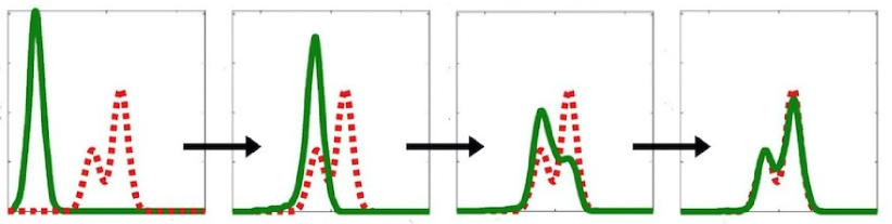
$\boldsymbol{{\color[rgb]{1,0,0}p}}$: target distribution;        $\boldsymbol{\color[rgb]{0,0.5,0}{q_{\ell}}}$: approximate distribution.

Figure 2: Evolution of the transformed density functions in SVGD. The target distribution in red dash line is an GMM with two modals. The initial distribution $q_{0}$ is transported by the transformation constructed by SVGD.

In the view of measure transport, SVGD iteratively transports the initial probability mass of the particles to the target distribution. SVGD constructs a path of distributions that bridges the initial distribution $q_{0}$ to the target distribution $p$ as follows,

$$q_{\ell}=({\boldsymbol{T}}_{\ell}\circ\cdots\circ{\boldsymbol{T}}_{1})\sharp q_{0},\quad\ell=1,\ldots,K.$$ (0.38)

where ${\boldsymbol{T}}\sharp q$ denotes the push-forward measure of $q$ through the transform ${\boldsymbol{T}}$, that is the distribution of $\boldsymbol{z}={\boldsymbol{T}}(\boldsymbol{x})$ when $\boldsymbol{x}\sim q$.

The story, however, is complicated by the fact that the transform ${\boldsymbol{T}}_{\ell}$ is practically constructed on the fly depending on the recent particles $\{{\boldsymbol{x}}_{i}^{\ell-1}\}_{i=1}^{n}$, which introduces complex dependency between the particles at the next iteration, whose theoretical understanding requires mathematical tools in interacting particle systems (e.g., Braun & Hepp, 1977; Spohn, 2012; Del Moral, 2013) and propagation of chaos (e.g., Sznitman, 1991). As a result, $\{\boldsymbol{x}_{i}^{\ell}\}_{i=1}^{n}$ can not be viewed as i.i.d. samples from $q_{\ell}$.

This makes it difficult to analyze the results of SVGD and quantify their bias and variance. In this paper, we propose a simple modification of SVGD that “decouples” the particle interaction and returns particles i.i.d. drawn from $q_{\ell}$; we also develop a method to iteratively keep track of the importance weights of these particles, which makes it possible to give consistent, or unbiased estimators within finite number of iterations of SVGD.

Our method integrates SVGD with importance sampling (IS) and combines their advantages: it leverages the SVGD dynamics to obtain high quality proposals $q_{\ell}$ for IS and also turns SVGD into a standard IS algorithm, inheriting the interpretability and theoretical properties of IS. Another advantage of our proposed method is that it provides an SVGD-based approach for estimating intractable normalization constants, an inference problem that the original SVGD does not offer to solve.

The proposals $q_{\ell}$ in our method, however, are obtained by recursive variable transforms constructed in a nonparametric fashion and become more complex as more transforms ${\boldsymbol{T}}_{\ell}$ are applied. In fact, one can view $q_{\ell}$ as the result of pushing $q_{0}$ through a neural network with $\ell$-layers, constructed in a non-parametric, layer-by-layer fashion, which provides a much more flexible distribution family than typical parametric families such as mixtures or exponential families.

There has been a collection of recent works, (such as Rezende & Mohamed, 2015; Kingma et al., 2016; Marzouk et al., 2016; Spantini et al., 2017), that approximate the target distributions with complex proposals obtained by iterative variable transforms in a similar way to our proposals $q_{\ell}$ in (0.38). The key difference, however, is that these methods explicitly parameterize the transforms ${\boldsymbol{T}}_{\ell}$ and optimize the parameters by back-propagation, while our method, by leveraging the nonparametric nature of SVGD, constructs the transforms ${\boldsymbol{T}}_{\ell}$ sequentially in closed forms, requiring no back-propagation. We introduce the basic idea of Stein variational gradient descent (SVGD) and Stein discrepancy. The readers are referred to Liu & Wang (2016) and Liu et al. (2016) for more detailed introduction.

Stein Discrepancy as Gradient of KL Divergence

Let $p({\boldsymbol{x}})$ be a density function on $\mathbb{R}^{d}$ which we want to approximate. We assume that we know $p({\boldsymbol{x}})$ only up to a normalization constant, that is,

$$p({\boldsymbol{x}})=\frac{1}{Z}\bar{p}({\boldsymbol{x}}),~{}~{}~{}~{}~{}Z=\int\bar{p}({\boldsymbol{x}})d{\boldsymbol{x}},$$ (0.39)

where we assume we can only calculate $\bar{p}({\boldsymbol{x}})$ and $Z$ is a normalization constant (known as the partition function) that is intractable to calculate exactly. We assume that $\log p({\boldsymbol{x}})$ is differentiable w.r.t. ${\boldsymbol{x}}$, and we have access to $\nabla\log p({\boldsymbol{x}})=\nabla\log\bar{p}({\boldsymbol{x}})$ which does not depend on $Z$.

The main idea of SVGD is to use a set of sequential deterministic transforms to iteratively push a set of particles $\{{\boldsymbol{x}}_{i}\}_{i=1}^{n}$ towards the target distribution:

$$\begin{split}&{\boldsymbol{x}}_{i}\leftarrow{\boldsymbol{T}}({\boldsymbol{x}}_{i}),~{}~{}~{}~{}\quad\forall i=1,2,\cdots,n\\ &{\boldsymbol{T}}({\boldsymbol{x}})=\boldsymbol{x}+\epsilon\boldsymbol{\phi}(\boldsymbol{x}),\end{split}$$ (0.40)

where we choose the transform ${\boldsymbol{T}}$ to be an additive perturbation by a velocity field ${\boldsymbol{\phi}}$, with a magnitude controlled by a step size $\epsilon$ that is assumed to be small.

The key question is the choice of the velocity field ${\boldsymbol{\phi}}$; this is done by choosing ${\boldsymbol{\phi}}$ to maximally decrease the $\mathrm{KL}$ divergence between the distribution of particles and the target distribution. Assume the current particles are drawn from $q$, and ${\boldsymbol{T}}\sharp q$ is the distribution of the updated particles, that is, ${\boldsymbol{T}}\sharp q$ is the distribution of $\boldsymbol{{\boldsymbol{x}}}^{\prime}={\boldsymbol{T}}({\boldsymbol{x}})=\boldsymbol{{\boldsymbol{x}}}+\epsilon\boldsymbol{\phi}(\boldsymbol{{\boldsymbol{x}}})$ when ${\boldsymbol{x}}\sim q$. The optimal ${\boldsymbol{\phi}}$ should solve the following functional optimization:

$$\begin{split}\mathbb{D}(q~{}||~{}p)\overset{def}{=}\max_{\boldsymbol{\phi}\in\mathcal{\mathcal{F}}\colon||{\boldsymbol{\phi}}||_{\mathcal{F}}\leq 1}\bigg{\{}-\frac{d}{d\epsilon}\mathrm{KL}({\boldsymbol{T}}\sharp q\mid\mid p)~{}\big{|}_{\epsilon=0}\bigg{\}},\end{split}$$ (0.41)

where $\mathcal{F}$ is a vector-valued normed function space that contains the set of candidate velocity fields ${\boldsymbol{\phi}}$.

The maximum negative gradient value $\mathbb{D}(q~{}||~{}p)$ in (0.41) provides a discrepancy measure between two distributions $q$ and $p$ and is known as Stein discrepancy (Gorham & Mackey, 2015; Liu et al., 2016; Chwialkowski et al., 2016): if $\mathcal{F}$ is taken to be large enough, we have $\mathbb{D}(q~{}||~{}p)=0$ iff there exists no transform to further improve the KL divergence between $p$ and $q$, namely $p=q$.

It is necessary to use an infinite dimensional function space $\mathcal{F}$ to obtain good transforms, which then casts a challenging functional optimization problem. Fortunately, it turns out that a simple closed form solution can be obtained by taking $\mathcal{F}$ to be an RKHS $\mathcal{H}=\mathcal{H}_{0}\times\cdots\mathcal{H}_{0}$, where $\mathcal{H}_{0}$ is a RKHS of scalar-valued functions, associated with a positive definite kernel $k(x,x^{\prime})$. In this case, Liu et al. (2016) showed that the optimal solution of (0.41) is ${\boldsymbol{\phi}}^{*}/||{\boldsymbol{\phi}}^{*}||_{\mathcal{H}}$, where

$$\boldsymbol{\phi}^{*}(\cdot)=\mathbb{E}_{\boldsymbol{x}\sim{q}}[\nabla_{\boldsymbol{x}}\log p(\boldsymbol{x})k(\boldsymbol{x},\cdot)+\nabla_{\boldsymbol{x}}k(\boldsymbol{x},\cdot)].$$ (0.42)

In addition, the corresponding Stein discrepancy, known as kernelized Stein discrepancy (KSD) (Liu et al., 2016; Chwialkowski et al., 2016; Gretton et al., 2009; Oates et al., 2016), can be shown to have the following closed form

$$\mathbb{D}(q~{}||~{}p)=||{\boldsymbol{\phi}}^{*}||_{\mathcal{H}}=\big{(}\mathbb{E}_{x,x^{\prime}\sim q}[\kappa_{p}({\boldsymbol{x}},{\boldsymbol{x}}^{\prime})]\big{)}^{1/2},$$ (0.43)

where $\kappa_{p}(x,x^{\prime})$ is a positive definite kernel defined by

$$\kappa_{p} (\boldsymbol{x},\boldsymbol{x}^{\prime})=\boldsymbol{s}_{p}(\boldsymbol{x})^{\top}k(\boldsymbol{x},\boldsymbol{x}^{\prime})\boldsymbol{s}_{p}(\boldsymbol{x}^{\prime})+\boldsymbol{s}_{p}(\boldsymbol{x})^{\top}\nabla_{\boldsymbol{x}^{\prime}}k(\boldsymbol{x},\boldsymbol{x}^{\prime})$$

$$+\boldsymbol{s}_{p}(\boldsymbol{x}^{\prime})^{\top}\nabla_{\boldsymbol{x}}k(\boldsymbol{x},\boldsymbol{x}^{\prime})+\nabla_{\boldsymbol{x}}\cdot(\nabla_{\boldsymbol{x}^{\prime}}k(\boldsymbol{x},\boldsymbol{x}^{\prime})).$$ (0.44)

where $\boldsymbol{s}_{p}({\boldsymbol{x}})\overset{def}{=}\nabla\log p({\boldsymbol{x}})$. We refer to Liu et al. (2016) for the derivation of (0.44), and further treatment of KSD in Chwialkowski et al. (2016); Oates et al. (2016); Gorham & Mackey (2017).

Complex Dependence of Particles in SVGD

In order to apply the derived optimal transform in the practical SVGD algorithm, we approximate the expectation $\mathbb{E}_{{\boldsymbol{x}}\sim q}[\cdot]$ in (0.42) using the empirical averaging of the current particles, that is, given particles $\{{\boldsymbol{x}}_{i}^{\ell}\}_{i=1}^{n}$ at the $\ell$-th iteration, we construct the following velocity field:

$$\!\!\!\!{\boldsymbol{\phi}}_{\ell+1}(\cdot)=\frac{1}{n}\sum_{j=1}^{n}[\nabla\log p(\boldsymbol{x}_{j}^{\ell})k(\boldsymbol{x}_{j}^{\ell},\cdot)+\nabla_{\boldsymbol{x}_{j}^{\ell}}k(\boldsymbol{x}_{j}^{\ell},\cdot)].$$ (0.45)

The SVGD update at the $\ell$-th iteration is then given by

$$\begin{split}&{\boldsymbol{x}}_{i}^{\ell+1}\leftarrow{\boldsymbol{T}}_{\ell+1}({\boldsymbol{x}}_{i}^{\ell}),\\ &{\boldsymbol{T}}_{\ell+1}({\boldsymbol{x}})={\boldsymbol{x}}+\epsilon{\boldsymbol{\phi}}_{\ell+1}({\boldsymbol{x}}).\end{split}$$ (0.46)

Here transform ${\boldsymbol{T}}_{\ell+1}$ is adaptively constructed based on the most recent particles $\{{\boldsymbol{x}}_{i}^{\ell}\}_{i=1}^{n}$. Assume the initial particles $\{{\boldsymbol{x}}_{i}^{0}\}_{i=1}^{n}$ are i.i.d. drawn from some distribution $q_{0}$, then the pushforward maps of ${\boldsymbol{T}}_{\ell}$ define a sequence of distributions that bridges between $q_{0}$ and $p$:

$$q_{\ell}=({\boldsymbol{T}}_{\ell}\circ\cdots\circ{\boldsymbol{T}}_{1})\sharp q_{0},\quad\ell=1,\ldots,K,$$ (0.47)

where $q_{\ell}$ forms increasingly better approximation of the target $p$ as $\ell$ increases. Because $\{{\boldsymbol{T}}_{\ell}\}$ are nonlinear transforms, $q_{\ell}$ can represent highly complex distributions even when the original $q_{0}$ is simple. In fact, one can view $q_{\ell}$ as a deep residual network (He et al., 2016) constructed layer-by-layer in a fast, nonparametric fashion.

However, because the transform ${\boldsymbol{T}}_{\ell}$ depends on the previous particles $\{{\boldsymbol{x}}_{i}^{\ell-1}\}_{i=1}^{n}$ as shown in (0.45), the particles $\{{\boldsymbol{x}}_{i}^{\ell}\}_{i=1}^{n}$, after the zero-th iteration, depend on each other in a complex fashion, and do not, in fact, straightforwardly follow distribution $q_{\ell}$ in (0.47). Principled approaches for analyzing such interacting particle systems can be found in Braun & Hepp (e.g., 1977); Spohn (e.g., 2012); Del Moral (e.g., 2013); Sznitman (e.g., 1991). The goal of this work, however, is to provide a simple method to “decouple” the SVGD dynamics, transforming it into a standard importance sampling method that is amendable to easier analysis and interpretability, and also applicable to more general inference tasks such as estimating partition function of unnormalized distribution where SVGD cannot be applied.

Stein Variational Adaptive Importance Sampling

In this section, we introduce our main Stein variational importance sampling (SteinIS) algorithm. Our idea is simple. We initialize the particles $\{{\boldsymbol{x}}_{i}^{0}\}_{i=1}^{n}$ by i.i.d. draws from an initial distribution $q_{0}$ and partition them into two sets, including a set of leader particles ${\boldsymbol{x}}_{A}^{\ell}=\{{\boldsymbol{x}}_{i}^{\ell}\colon i\in A\}$ and follower particles ${\boldsymbol{x}}_{B}^{\ell}=\{{\boldsymbol{x}}_{i}^{\ell}\colon i\in B\}$, with $B=\{1,\ldots,n\}\setminus A$, where the leader particles ${\boldsymbol{x}}_{A}^{\ell}$ are responsible for constructing the transforms, using the standard SVGD update (0.46), while the follower particles ${\boldsymbol{x}}_{B}^{\ell}$ simply follow the transform maps constructed by ${\boldsymbol{x}}_{A}^{\ell}$ and do not contribute to the construction of the transforms. In this way, the follower particles ${\boldsymbol{x}}_{B}^{\ell}$ are independent conditional on the leader particles ${\boldsymbol{x}}_{A}^{\ell}$.

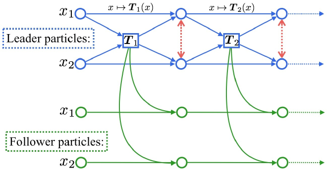
Figure 3: Illustrating the decoupled particles and their update in SteinIS. The leader particles set ${\boldsymbol{x}}_{A}^{\ell}$ is used to construct the transform $T_{\ell}$ and the follower particles ${\boldsymbol{x}}_{B}^{\ell}$ is updated by the constructed transform. The leader particles ${\boldsymbol{x}}_{A}^{\ell}$ are interactive and dependent on each other. The follower particles ${\boldsymbol{x}}_{B}^{\ell}$ can be viewed as i.i.d. draws from $q_{\ell}$, given fixed leader particles ${\boldsymbol{x}}_{A}^{\ell}$.

Conceptually, we can think that we first construct all the maps ${\boldsymbol{T}}_{\ell}$ by evolving the leader particles ${\boldsymbol{x}}_{A}^{\ell}$, and then push the follower particles through ${\boldsymbol{T}}_{\ell}$ in order to draw exact, i.i.d. samples from $q_{\ell}$ in (0.47). Note that this is under the assumption the leader particles ${\boldsymbol{x}}_{A}^{\ell}$ has been observed and fixed, which is necessary because the transform ${\boldsymbol{T}}_{\ell}$ and distribution $q_{\ell}$ depend on ${\boldsymbol{x}}_{A}^{\ell}$.

In practice, however, we can simultaneously update both the leader and follower particles, by a simple modification of the original SVGD (0.46),

$$\boldsymbol{x}_{i}^{\ell+1}\leftarrow\boldsymbol{x}_{i}^{\ell}+\epsilon{\boldsymbol{\phi}}_{\ell+1}(\boldsymbol{x}_{i}^{\ell}),~{}\forall i\in A\cup B,$$

$${\boldsymbol{\phi}}_{\ell+1}(\cdot)=\frac{1}{|A|}\sum_{j\in A}[\nabla\log p(\boldsymbol{x}_{j}^{\ell})k(\boldsymbol{x}_{j}^{\ell},\cdot)+\nabla_{\boldsymbol{x}_{j}^{\ell}}k(\boldsymbol{x}_{j}^{\ell},\cdot)].$$ (0.48)

where the only difference is that we restrict the empirical averaging in (0.45) to the set of the leader particles ${\boldsymbol{x}}_{A}^{\ell}$. The whole procedure is summarized in Algorithm 3. The relationship between the particles in set $A$ and $B$ can be more easily understood in Figure 3.

Algorithm 3 Stein Variational Importance Sampling

  Goal: Obtain i.i.d. importance sample $\{{\boldsymbol{x}}_{i}^{K},~{}w_{i}^{K}\}$ for $p$.

  Initialize ${\boldsymbol{x}}_{A}^{0}$ and ${\boldsymbol{x}}_{B}^{0}$ by i.i.d. draws from $q_{0}$.

  Calculate $\{q_{0}({\boldsymbol{x}}_{i}^{0})\},\forall i\in B.$

  for iteration $\ell=0,\ldots,K-1$ do

     1. Construct the map using the leader particles ${\boldsymbol{x}}_{A}^{\ell}$

$$\!\!\!\!\!\!\!\!{\boldsymbol{\phi}}_{\ell+1}(\cdot)=\frac{1}{|A|}\sum_{j\in A}[\nabla\log p(\boldsymbol{x}_{j}^{\ell})k(\boldsymbol{x}_{j}^{\ell},\cdot)+\nabla_{\boldsymbol{x}_{j}^{\ell}}k(\boldsymbol{x}_{j}^{\ell},\cdot)].$$

2. Update both the leader and follower particles

$$\boldsymbol{x}_{i}^{\ell+1}\leftarrow\boldsymbol{x}_{i}^{\ell}+\epsilon{\boldsymbol{\phi}}_{\ell+1}(\boldsymbol{x}_{i}^{\ell}),~{}~{}~{}~{}\forall i\in A\cup B.$$

3. Update the density values (for $i\in B$) by

$$q_{\ell+1}({\boldsymbol{x}}_{i}^{\ell+1})=q_{\ell}({\boldsymbol{x}}_{i}^{\ell})\cdot|\mathrm{det}(I~{}+~{}\epsilon\nabla_{\boldsymbol{x}}\boldsymbol{{\boldsymbol{\phi}}}_{\ell+1}(\boldsymbol{x}^{\ell}_{i}))|^{-1}$$

  end for

  Calcuate $w_{i}^{K}=p(\boldsymbol{x}_{i}^{K})/q_{K}(\boldsymbol{x}_{i}^{K}),\forall i\in B.$

  Outputs: i.i.d. importance sample $\{{\boldsymbol{x}}_{i}^{K},~{}w_{i}^{K}\}$ for $i\in B.$

Calculating the Importance Weights

Because $q_{\ell}$ is still different from $p$ when we only apply finite number of iterations $\ell$, which introduces deterministic biases if we directly use ${\boldsymbol{x}}_{B}^{\ell}$ to approximate $p$.

We address this problem by further turning the algorithm into an importance sampling algorithm with importance proposal $q_{\ell}$. Specifically, we calculate the importance weights of the particles $\{{\boldsymbol{x}}_{i}^{\ell}\}$:

$$w_{i}^{\ell}=\frac{\bar{p}({\boldsymbol{x}}_{i}^{\ell})}{q_{\ell}({\boldsymbol{x}}_{i}^{\ell})},$$ (0.49)

where $\bar{p}$ is the unnormalized density of $p$, that is, $p({\boldsymbol{x}})=\bar{p}({\boldsymbol{x}})/Z$ as in (0.39). In addition, the importance weights in (0.49) can be calculated based on the following formula:

$$q_{\ell}(\boldsymbol{x}^{\ell})=q_{0}(\boldsymbol{x}^{0})\prod_{\jmath=1}^{\ell}|\mathrm{det}(\nabla_{\boldsymbol{x}}\boldsymbol{T}_{\jmath}(\boldsymbol{x}^{\jmath-1}))|^{-1},$$ (0.50)

where $\boldsymbol{T}_{\ell}$ is defined in (0.46) and we assume that the step size $\epsilon$ is small enough so that each ${\boldsymbol{T}}_{\ell}$ is an one-to-one map. As shown in Algorithm 3 (step 3), (0.50) can be calculated recursively as we update the particles.

With the importance weights calculated, we turn SVGD into a standard importance sampling algorithm. For example, we can now estimate expectations of form $\mathbb{E}_{p}f$ by

$$\hat{\mathbb{E}}_{p}[f]=\frac{\sum_{i\in B}w_{i}^{\ell}f({\boldsymbol{x}}_{i}^{\ell})}{\sum_{i\in B}w_{i}^{\ell}},$$

which provides a consistent estimator of $\mathbb{E}_{p}f$ when we use finite number $\ell$ of transformations. Here we use the self normalized weights because $\bar{p}({\boldsymbol{x}})$ is unnormalized. Further, the sum of the unnormalized weights provides an unbiased estimation for the normalization constant $Z$:

$$\hat{Z}=\frac{1}{|B|}\sum_{i\in B}w_{i}^{\ell},$$

which satisfies the unbiasedness property $\mathbb{E}[\hat{Z}]=Z$. Note that the original SVGD does not provide a method for estimating normalization constants, although, as a side result of this work, Section 4 will discuss another method for estimating $Z$ that is more directly motivated by SVGD.

We now analyze the time complexity of our algorithm. Let $\alpha(d)$ be the cost of computing $\boldsymbol{s}_{p}(\boldsymbol{x})$ and $\beta(d)$ be the cost of evaluating kernel $k({\boldsymbol{x}},{\boldsymbol{x}}^{\prime})$ and its gradient $\nabla k({\boldsymbol{x}},{\boldsymbol{x}}^{\prime})$. Typically, both $\alpha(d)$ and $\beta(d)$ grow linearly with the dimension $d.$ In most cases, $\alpha(d)$ is much larger than $\beta(d)$. The complexity of the original SVGD with $|A|$ particles is $O(|A|\alpha(d)+|A|^{2}\beta(d))$, and the complexity of Algorithm 3 is $O(|A|\alpha(d)+|A|^{2}\beta(d)+|B||A|\beta(d)+|B|d^{3}),$ where the $O(|B|d^{3})$ complexity comes from calculating the determinant of the Jacobian matrix, which is expensive when dimension $d$ is high, but is the cost to pay for having a consistent importance sampling estimator in finite iterations and for being able to estimate the normalization constant $Z$. Also, by calculating the effective sample size based on the importance weights, we can assess the accuracy of the estimator, and early stop the algorithm when a confidence threshold is reached.

One way to speed up our algorithm in empirical experiments is to parallelize the computation of Jacobian matrices for all follower particles in GPU. It is possible, however, to develop efficient approximation for the determinants by leveraging the special structure of the Jacobean matrix; note that

$$\nabla_{\boldsymbol{y}}\boldsymbol{T}(\boldsymbol{y})=I+\epsilon A,$$

$$A=\frac{1}{n}\sum_{j=1}^{n}[\nabla_{\boldsymbol{x}}\log p(\boldsymbol{x}_{j})^{\top}\nabla_{\boldsymbol{y}}k(\boldsymbol{x}_{j},\boldsymbol{y})+\nabla_{\boldsymbol{x}}\nabla_{\boldsymbol{y}}k(\boldsymbol{x}_{j},\boldsymbol{y})].$$

Therefore, $\nabla_{\boldsymbol{y}}\boldsymbol{T}(\boldsymbol{y})$ is close to the identity matrix $I$ when the step size is small. This allows us to use Taylor expansion for approximation:

Proposition 2.

Assume $\epsilon<1/\rho(A)$, where $\rho(A)$ is the spectral radius of $A$, that is, $\rho(A)=\max_{j}|\lambda_{j}(A)|$ and $\{\lambda_{j}\}$ are the eigenvalues of $A$. We have

$$\mathrm{det}(I+\epsilon A)=\prod_{k=1}^{d}(1+\epsilon a_{kk})+O(\epsilon^{2}),$$ (0.51)

where $\{a_{kk}\}$ are the diagonal elements of $A$.

Proof.

Use the Taylor expansion of $\mathrm{det}(I+\epsilon A)$. Note that $\mathrm{det}(I+\epsilon A)=\exp(\mathrm{trace}(\log(I+\epsilon A))),$ and $\log(I+\epsilon A)=1+\epsilon A+O(\epsilon^{2}).$ and $\log(I+\epsilon A)=\sum_{n=1}^{\infty}\frac{(-1)^{n-1}}{n}\epsilon^{n}A^{n},$ where $A^{n}=A^{n-1}A.$ T $\mathrm{det}(I+\epsilon A)=\prod_{k}^{d}(1+\epsilon a_{kk})+O(\epsilon^{2}).$ ∎

Therefore, one can approximate the determinant with approximation error $O(\epsilon^{2})$ using linear time $O(d)$ w.r.t. the dimension. Often the step size is decreasing with iterations, and a way to trade-off the accuracy with computational cost is to use the exact calculation in the beginning when the step size is large, and switch to the approximation when the step size is small.

The idea of constructing a path of distributions $\{q_{\ell}\}$ to bridge the target distribution $p$ with a simpler distribution $q_{0}$ invites connection to ideas such as annealed importance sampling (AIS) (Neal, 2001) and path sampling (PS) (Gelman & Meng, 1998). These methods typically construct an annealing path using geometric averaging of the initial and target densities instead of variable transforms, which does not build in a notion of variational optimization as the SVGD path. In addition, it is often intractable to directly sample distributions on the geometry averaging path, and hence AIS and PS need additional mechanisms in order to construct proper estimators.

Monotone Decreasing of KL divergence

One nice property of algorithm 3 is that the KL divergence between the iterative distribution $q_{\ell}$ and $p$ is monotonically decreasing. This property can be more easily understood by considering our iterative system in continuous evolution time as shown in Liu (2017). Take the step size $\epsilon$ of the transformation defined in (0.40) to be infinitesimal, and define the continuos time $t=\epsilon\ell$. Then the evolution equation of random variable ${\boldsymbol{x}}^{t}$ is governed by the following nonlinear partial differential equation (PDE),

$$\frac{d\boldsymbol{x}^{t}}{dt}=\mathbb{E}_{\boldsymbol{x}\sim{q_{t}}}[\boldsymbol{s}_{p}(\boldsymbol{x})k(\boldsymbol{x},\boldsymbol{x}^{t})+\nabla_{\boldsymbol{x}}k(\boldsymbol{x},\boldsymbol{x}^{t})],$$ (0.52)

where $t$ is the current evolution time and $q_{t}$ is the density function of ${\boldsymbol{x}}^{t}.$ The current evolution time $t=\epsilon\ell$ when $\epsilon$ is small and $\ell$ is the current iteration. We have the following proposition (see also Liu (2017)):

Proposition 3.

Suppose random variable $\boldsymbol{x}^{t}$ is governed by PDE (0.182), then its density $q_{t}$ is characterized by

$$\frac{\partial q_{t}}{\partial t}=-\mathrm{div}(q_{t}\mathbb{E}_{\boldsymbol{x}\sim{q_{t}}}[\boldsymbol{s}_{p}(\boldsymbol{x})k(\boldsymbol{x},\boldsymbol{x}^{t})+\nabla_{\boldsymbol{x}}k(\boldsymbol{x},\boldsymbol{x}^{t})]),$$ (0.53)

where $\mathrm{div}(\boldsymbol{f})=\mathrm{trace}(\nabla\boldsymbol{f})=\sum_{i=0}^{d}\partial f_{i}(\boldsymbol{x})/\partial x_{i}$, and $\boldsymbol{f}=[f_{1},\ldots,f_{d}]^{\top}.$

The proof of proposition 3 is similar to the proofs of proposition 1.1 in Jourdain & Méléard (1998) and lemma 1 in dai2019opaque. Proposition 3 characterizes the evolution of the density function $q_{t}(\boldsymbol{x}^{t})$ when the random variable $\boldsymbol{x}^{t}$ is evolved by  (0.182). The continuous system captured by (0.182) and  (0.157) is a type of Vlasov process which has wide applications in physics, biology and many other areas (e.g., Braun & Hepp, 1977). As a consequence of proposition 3, one can show the following nice property:

$$\frac{d\mathrm{KL}(q_{t}\mid\mid p)}{dt}=-\mathbb{D}(q_{t}~{}||~{}p)^{2}<0,$$ (0.54)

which is proved by theorem 4.4 in Liu (2017). Equation  (0.166) indicates that the KL divergence between the iterative distribution $q_{t}$ and $p$ is monotonically decreasing with a rate of $\mathbb{D}(q_{t}~{}||~{}p)^{2}$.

A Path Integration Method

Algorithm 4 SVGD with Path Integration for estimating $\mathrm{KL}(q_{0}~{}||~{}p)$ and $\log Z$

1:  Input: Target distribution $p(x)=\bar{p}(x)/Z$; an initial distribution $q_{0}$.

2:  Goal: Estimating $\mathrm{KL}(q_{0}\mid\mid p)$ and the normalization constant $\log Z.$

3:   Initialize $\hat{K}=0.$ Initialize particles $\{{\boldsymbol{x}}_{i}^{0}\}_{i=1}^{n}\sim q_{0}(\boldsymbol{x}).$

4:  Compute $\hat{\mathbb{E}}_{q_{0}}[\log(q_{0}({\boldsymbol{x}})/\overline{p}({\boldsymbol{x}}))]$ via sampling from $q_{0}.$

5:  while iteration $\ell$ do

6:     

$$\hat{K}\leftarrow\hat{K}+\epsilon\hat{\mathbb{D}}({q}_{\ell}~{}||~{}p)^{2},$$

$${\boldsymbol{x}}_{i}^{\ell+1}\leftarrow{\boldsymbol{x}}_{i}^{\ell}+\boldsymbol{\phi}_{\ell+1}({\boldsymbol{x}}_{i}^{\ell}),$$

where $\hat{\mathbb{D}}({q}_{\ell}~{}||~{}p)$ is defined in (0.57).

7:  end while

8:  Estimate $\mathrm{KL}(q_{0}~{}||~{}p)$ by $\hat{K}$ and $\log Z$ by $\hat{\mathbb{D}}-\hat{\mathbb{E}}_{q_{0}}[\log(q_{0}({\boldsymbol{x}})/\overline{p}({\boldsymbol{x}}))].$

We mentioned that the original SVGD does not have the ability to estimate the partition function. Section 3 addressed this problem by turning SVGD into a standard importance sampling algorithm in Section 3. Here we introduce another method for estimating KL divergence and normalization constants that is more directly motivated by the original SVGD, by leveraging the fact that the Stein discrepancy is a type of gradient of KL divergence. This method does not need to estimate the importance weights but has to run SVGD to converge to diminish the Stein discrepancy between intermediate distribution $q_{\ell}$ and $p$. In addition, this method does not perform as well as Algorithm 1 as we find empirically. Nevertheless, we find this idea is conceptually interesting and useful to discuss it.

Recalling equation (0.41) in Section 2.1, we know that if we perform transform ${\boldsymbol{T}}({\boldsymbol{x}})={\boldsymbol{x}}+\epsilon{\boldsymbol{\phi}}^{*}({\boldsymbol{x}})$ with ${\boldsymbol{\phi}}^{*}$ defined in (0.42), the corresponding decrease of KL divergence would be

$$\begin{split}\mathrm{KL}(q~{}||~{}p)-\mathrm{KL}({\boldsymbol{T}}\sharp q~{}||~{}p)&\approx\epsilon\cdot||{\boldsymbol{\phi}}^{*}||_{\mathcal{H}}\cdot\mathbb{D}(q~{}||~{}p)\\ &\approx\epsilon\cdot\mathbb{D}(q~{}||~{}p)^{2},\end{split}$$ (0.55)

where we used the fact that $\mathbb{D}(q~{}||~{}p)=||{\boldsymbol{\phi}}^{*}||_{\mathcal{H}}$, shown in (0.43). Applying this recursively on $q_{\ell}$ in (0.55), we get

$$\mathrm{KL}(q_{0}~{}||~{}p)-\mathrm{KL}(q_{\ell+1}~{}||~{}p)\approx\sum_{\jmath=0}^{\ell}\epsilon\cdot\mathbb{D}(q_{\jmath}~{}||~{}p)^{2}.$$

Assuming $\mathrm{KL}(q_{\ell}~{}||~{}p)\to 0$ when $\ell\to\infty$, we get

$$\mathrm{KL}(q_{0}~{}||~{}p)\approx\sum_{\ell=0}^{\infty}\epsilon\cdot\mathbb{D}(q_{\ell}~{}||~{}p)^{2}.$$ (0.56)

By (0.43), the square of the KSD can be empirically estimated via V-statistics, which is given as

$$\hat{\mathbb{D}}(q_{\ell}~{}||~{}p)^{2}=\frac{1}{n^{2}}\sum_{i=1}^{n}\sum_{j=1}^{n}\kappa({\boldsymbol{x}}_{i}^{\ell},{\boldsymbol{x}}_{j}^{\ell}).$$ (0.57)

Overall, equation (0.56) and (0.57) give an estimator of the KL divergence between $q_{0}$ and $p=\bar{p}(\boldsymbol{x})/Z.$ This can be transformed into an estimator of the log normalization constant $\log Z$ of $p$, by noting that

$$\log Z=\mathrm{KL}(q_{0}\mid\mid p)-\mathbb{E}_{q_{0}}[\log(q_{0}({\boldsymbol{x}})/\overline{p}({\boldsymbol{x}}))],$$ (0.58)

where the second term can be estimated by drawing a lot of samples to diminish its variance since the samples from $q_{0}$ is easy to draw. The whole procedure is summarized in Algorithm 4.

Empirical Experiments of SteinIS

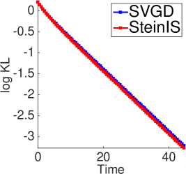
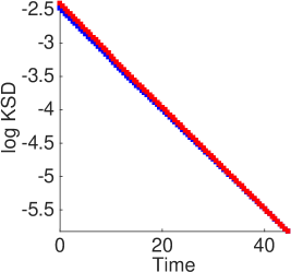
(a) KL	(b) KSD

Figure 4: Verifying the monotone deceasing of $\mathrm{KL}$ divergence in SteinIS on GMM with 10 mixture components. $d=1.$ In SVGD, 500 particles are evolved. In SteinIS, $|A|=200$ and $|B|=500$. For SVGD and SteinIS, all particles are drawn from the same Gaussian distribution $q_{0}(\boldsymbol{x}).$

We study the empirical performance of our proposed algorithms on both simulated and real world datasets. We start with toy examples to numerically investigate some theoretical properties of our algorithms, and compare it with traditional adaptive IS on non-Gaussian, multi-modal distributions. We also employ our algorithm to estimate the partition function of Gaussian-Bernoulli Restricted Boltzmann Machine(RBM), a graphical model widely used in deep learning (Welling et al., 2004; Hinton & Salakhutdinov, 2006), and to evaluate the log likelihood of decoder models in variational autoencoder (Kingma & Welling, 2013).

We summarize some hyperparameters used in our experiments. We use RBF kernel $k(\boldsymbol{x},\boldsymbol{x}^{\prime})=\exp(-\|\boldsymbol{x}-\boldsymbol{x}^{\prime}\|^{2}/h),$ where $h$ is the bandwidth. In most experiments, we let $h{=}\mathrm{med^{2}}/(2\log(|A|+1))$, where $\mathrm{med}$ is the median of the pairwise distance of the current leader particles ${\boldsymbol{x}}_{A}^{\ell}$, and $|A|$ is the number of leader particles. The step sizes in our algorithms are chosen to be $\epsilon=\alpha/(1+\ell)^{\beta},$ where $\alpha$ and $\beta$ are hyperparameters chosen from a validation set to achieve best performance. When $\epsilon\leq 0.1$, we use first-order approximation to calculate the determinants of Jacobian matrices as illustrated in proposition 2.

In what follows, we use “AIS” to refer to the annealing importance sampling with Langevin dynamics as its Markov transitions, and use “HAIS” to denote the annealing importance sampling whose Markov transition is Hamiltonian Monte Carlo (HMC). We use ”transitions” to denote the number of intermediate distributions constructed in the paths of both SteinIS and AIS. A transition of HAIS may include $L$ leapfrog steps, as implemented by  Wu et al. (2016).

Verification of Monotone Decreasing of KL Divergence in SteinIS

We start with testing our methods on simple 2 dimensional Gaussian mixture models with 10 randomly generated mixture components. The dimension of ${\boldsymbol{x}}$ in $p({\boldsymbol{x}})$ is one. In SVGD, 500 particles are evolved. In SteinIS, the leader particle set size $|A|=200$ and the follower particle set size $|B|=500$. For SVGD and SteinIS, all particles are drawn from the same Gaussian distribution $q_{0}(\boldsymbol{x}).$ First, we numerically investigate the convergence of KL divergence between the particle distribution $q_{t}$ (in continuous time) and $p.$ Sufficient particles are drawn and infinitesimal step $\epsilon$ is taken to closely simulate the continuous time system, as defined by (0.182), (0.157) and (0.166). Figure 4(a)-(b) show that the KL divergence $\mathrm{KL}(q_{t},p)$, as well as the squared Stein discrepancy $\mathbb{D}(q_{t},p)^{2}$, seem to decay exponentially in both SteinIS and the original SVGD. This suggests that the quality of our importance proposal $q_{t}$ improves quickly as we apply sufficient transformations. However, it is still an open question to establish the exponential decay theoretically; see Liu (2017) for a related discussion.

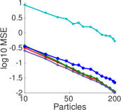
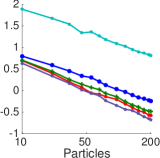
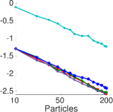
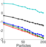
(a) $\mathbb{E}[x]$	(b) $\mathbb{E}[x^{2}]$	(c) $\mathbb{E}[\cos(wx+b)]$	(d) Partition Function

Figure 5: Verification of the convergence rate of SteinIS w.r.t. the sample size on 2D GMM with 10 randomly generated mixture components. $d=2.$ (a)-(c) shows mean square error(MSE) for estimating $\mathbb{E}_{p}[h(x)],$ where $h(\boldsymbol{x})=x_{j},~{}x_{j}^{2},~{}\cos(wx_{j}+b),$ for $j=1,2.$ 800 transitions are used in SteinIS, HAIS and AIS. L=1 in HAIS. The size of leader particles $|A|$ is fixed as 100 and let the size of follower particles $|B|$ vary in SteinIS. The initial proposal $q_{0}(\boldsymbol{x})$ is Gaussian. ”Direct” means that samples are directly drawn from $p(\boldsymbol{x})$ and is not applicable in (d). ”IS” means we directly draw samples from $q_{0}.$ ”Path” denotes the proposed algorithm 4 and is only applicable to estimate (d). The MSE is averaged on each coordinate over 500 independent experiments for SteinIS, HAIS, AIS and Direct, and over 2000 independent experiments for IS. SVGD has similar resluts as our SteinIS on (a), (b), (c) and is not provided in this figure for clarity. SVGD cannot be applied to task (d). The logarithm base is 10.

Verification of Convergence Property of SteinIS

We also empirically verify the convergence of our SteinIS as the follower particle size $|B|$ increases (as the leader particle size $|A|$ is fixed) in Fig. 5. We apply SteinIS to estimate $\mathbb{E}_{p}[h(x)],$ where $h(\boldsymbol{x})=x_{j},~{}x_{j}^{2}~{}\textit{or}~{}\cos(wx_{j}+b)$ with $w\sim\mathcal{N}(0,1)$ and $b\sim\mathrm{Uniform}([0,1])$ for $j=1,2$, and the partition function (which is trivially $1$ in this case). In Fig. 5(a)-(c) shows mean square error(MSE) for estimating $\mathbb{E}_{p}[h(x)],$ where $h(\boldsymbol{x})=x_{j},~{}x_{j}^{2},~{}\cos(wx_{j}+b)$ with $w\sim\mathcal{N}(0,1)$ and $b\in\mathrm{Uniform}([0,1])$ for $j=1,2$, and the normalization constant (which is $1$ in this case). From Fig. 5, we can see that the mean square error(MSE) of our algorithms follow the typical convergence rate of IS, which is $O(1/\sqrt{|B|}),$ where $|B|$ is the number of samples for performing IS. Figure 5 indicates that SteinIS can achieve almost the same performance as the exact Monte Carlo (which directly draws samples from the target $p({\boldsymbol{x}})$), indicating the proposal $q_{\ell}({\boldsymbol{x}})$ closely matches the target $p({\boldsymbol{x}})$.

We used 800 transitions in SteinIS, HAIS and AIS, and take $L=1$ in HAIS. We fixed the size of the leader particles $|A|$ to be $100$ and vary the size of follower particles $|B|$ in SteinIS. The initial proposal $q_{0}$ is the standard Gaussian. ”Direct” means that samples are directly drawn from $p$ and is not applicable in (d). ”IS” means we directly draw samples from $q_{0}$ and apply standard importance sampling. ”Path” denotes path integration method in Algorithm 4 and is only applicable to estimate the partition function in (d). The MSE is averaged on each coordinate over 500 independent experiments for SteinIS, HAIS, AIS and Direct, and over 2000 independent experiments for IS. SVGD has similar results (not shown for clarity) as our SteinIS on (a), (b), (c), but can not be applied to estimate the partition function in task (d). The logarithm base is 10.

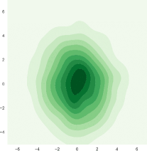
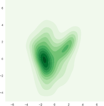
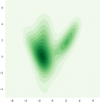
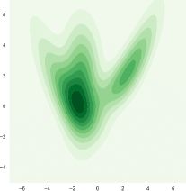
(a) SteinIS, $\ell=0$	(b) SteinIS, $\ell=50$	(c) SteinIS, $\ell=200$	(d) SteinIS, $\ell=2000$
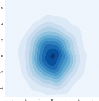
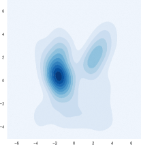
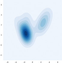
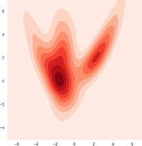
(e)Adap IS, $\ell=0$	(f)Adap IS, $\ell=1000$	(g)Adap IS, $\ell=10000$	(h) Exact

Figure 6: Evolution of the contour of density functions for SteinIS and Adaptive IS. The top line shows the contours of the evolved density functions in SteinIS, i.e., (a, b, c, d). (e, f, g) are the evolved contours of the traditional adaptive IS. (h) is the contour of the target density $p(\boldsymbol{x})$. The number of mixture components for adaptive IS is 200 and the number of leader particles for approximating the map in SteinIS is 200.

Comparison between SteinIS and Adaptive IS

In the following, we compare SteinIS with traditional adaptive IS (Ryu & Boyd, 2014) on a probability model $p(\boldsymbol{x})$, obtained by applying nonlinear transform on a three-component Gaussian mixture model.

Specifically, let $\widetilde{q}$ be a 2D Gaussian mixture model, and $\boldsymbol{T}$ is a nonlinear transform defined by $\boldsymbol{T}(\boldsymbol{z})=[a_{1}z_{1}+b_{1},a_{2}z_{1}^{2}+a_{3}z_{2}+b_{2}]^{\top}$, where $\boldsymbol{z}=[z_{1},z_{2}]^{\top}.$ We define the target $p$ to be the distribution of ${\boldsymbol{x}}=\boldsymbol{T}(\boldsymbol{z})$ when $\boldsymbol{z}\sim\widetilde{q}$.

The contour of the target density $p$ we constructed is shown in Figure 6(h). We test our SteinIS and visualize in Figure 6(a)-(d) the density of the evolved distribution $q_{\ell}$ using kernel density estimation, by drawing a large number of follower particles at iteration equaling $0$, $50$, $200$, $1000$ respectively. We compare our method with the adaptive IS by (Ryu & Boyd, 2014) using a proposal family formed by Gaussian mixture with $200$ components. The densities of the proposals obtained by adaptive IS at different iterations are shown in Figure 6(e)-(g) at iteration equaling $0$, $1000$, $10000$ respectively. The number of the mixture components for adaptive IS is $200$ and the number of leader particles for approximating the map in SteinIS is also $200$.

We can see that the evolved proposals of SteinIS converge to the target density $p(\boldsymbol{x})$ and approximately match $p(\boldsymbol{x})$ at 2000 iterations, but the optimal proposal of adaptive IS with 200 mixture components (at the convergence) can not fit $p(\boldsymbol{x})$ well, as indicated by Figure 6(g). This is because the Gaussian mixture proposal family (even with upto 200 components) can not closely approximate the non-Gaussian target distribution we constructed. We should remark that SteinIS can be applied to refine the optimal proposal given by adaptive IS to get better importance proposal by implementing a set of successive transforms on the given IS proposal.

Qualitatively, we find that the KL divergence (calculated via kernel density estimation) between our evolved proposal $q_{\ell}$ and $p$ decreases to $\leq 0.003$ after 2000 iterations, while the KL divergence between the optimal adaptive IS proposal and the target $p$ can be only decreased to $0.42$ even after sufficient optimization.

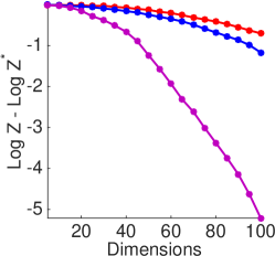
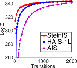
(a) Vary dimensions	(b) 100 dimensions

Figure 7: Gauss-Bernoulli RBM with $d^{\prime}=10$. The initial distribution $q_{0}(\boldsymbol{x})$ for SteinIS, HAIS and AIS is multivariate Gaussian. We let $|A|=100$ in SteinIS and use 100 samples for implementing IS in SteinIS, HAIS and AIS. In (a), we use 1500 transitions for HAIS, SteinIS and AIS. ”HAIS-1L” means $L=1$ in each Markov transition of HAIS. SVGD is not applicable. $\log Z^{*}$ denotes the logarithm of the exact normalizing constant. All experiments are averaged over 500 independent trails.

Gauss-Bernoulli Restricted Boltzmann Machine

We apply our method to estimate the partition function of Gauss-Bernoulli Restricted Boltzmann Machine (RBM), which is a multi-modal, hidden variable graphical model. Effective estimation of the partition function is a fundamental task on the application of probabilistic graphical model (Liu et al., 2015b). It consists of a continuous observable variable $\boldsymbol{x}\in\mathbb{R}^{d}$ and a binary hidden variable $\boldsymbol{h}\in\{\pm 1\}^{d^{\prime}},$ with a joint probability density function of form

$$p(\boldsymbol{x},\boldsymbol{h})=\frac{1}{Z}\exp(\boldsymbol{x}^{\mathrm{T}}B\boldsymbol{h}+b^{\mathrm{T}}\boldsymbol{x}+c^{\mathrm{T}}\boldsymbol{h}-\frac{1}{2}\|\boldsymbol{x}\|_{2}^{2}),$$ (0.59)

where $p(\boldsymbol{x})=\frac{1}{Z}\sum_{\boldsymbol{h}}p(\boldsymbol{x},\boldsymbol{h})$ and $Z$ is the normalization constant. By marginalzing the hidden variable $h$, we can show that $p(\boldsymbol{x})$ is

$$p(\boldsymbol{x})=\frac{1}{Z}\exp(b^{\mathrm{T}}\boldsymbol{x}-\frac{1}{2}\|\boldsymbol{x}\|_{2}^{2})\prod_{i=1}^{d^{\prime}}[\exp(\varphi_{i})+\exp(-\varphi_{i})],$$

where $\varphi=B^{\mathrm{T}}\boldsymbol{x}+c$, and its score function $\boldsymbol{s}_{p}$ is easily derived as

$$\boldsymbol{s}_{p}(\boldsymbol{x})=\nabla_{\boldsymbol{x}}\log p(\boldsymbol{x})=b-\boldsymbol{x}+B\frac{\exp(2\varphi)-1}{\exp(2\varphi)+1}.$$

In our experiments, we simulate a true model $p(\boldsymbol{x})$ by drawing $b$ and $c$ from the standard Gaussian distribution and select $B$ uniformly random from $\{0.5,-0.5\}$ with probability 0.5. The dimension of the latent variable $\boldsymbol{h}$ is 10 so that the probability model $p(\boldsymbol{x})$ is the mixture of $2^{10}$ multivariate Gaussian distribution. The exact normalization constant $Z$ can be feasibly calculated using the brute-force algorithm in this case. The initial distribution $q_{0}(\boldsymbol{x})$ for all the methods is a same multivariate Gaussian. We let $|A|=100$ in SteinIS and use $(B=)$100 importance samples in SteinIS, HAIS and AIS. In (a), we use 1500 transitions for HAIS, SteinIS and AIS. ”HAIS-1L” means we use $L=1$ leapfrog in each Markov transition of HAIS. $\log Z^{*}$ denotes the logarithm of the exact normalizing constant. All experiments are averaged over 500 independent trails. Figure 7(a) and Figure 7(b) shows the performance of SteinIS on Gauss-Bernoulli RBM when we vary the dimensions of the observed variables and the number of transitions in SteinIS, respectively. We can see that SteinIS converges slightly faster than HAIS which uses one leapfrog step in each of its Markov transition. Even with the same number of Markov transitions, AIS with Langevin dynamics converges much slower than both SteinIS and HAIS. The better performance of HAIS comparing to AIS was also observed by  Sohl-Dickstein & Culpepper (2012) when they first proposed Hamiltonian annealed importance sampling.

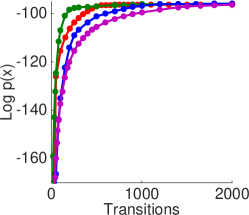
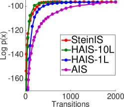
(a) 20 hidden variables	(b) 50 hidden variables

Figure 8: Evaluation of the testing log-likelihood $\log p(x)$ for the decoder-based generative models generative model on MNIST dataset. The initial distribution $q_{0}(\boldsymbol{z})$ for SteinIS, HAIS and AIS is multivariate Gaussian. We let $|A|=60$ in SteinIS and use 60 samples for each image to implement IS in SteinIS, HAIS and AIS. ”HAIS-10L” and ”HAIS-1L” denote $L=10$ and $L=1$ in each Markov transition of HAIS respectively. The log-likelihood is calculated over 1000 images randomly chosen from MNIST. The dimensions in (a) and (b) are the dimensions of latent space $\boldsymbol{z}$ in our setting.

Deep Generative Models

Finally, we implement our SteinIS to evaluate the $\log$-likelihoods of the decoder models in variational autoencoder (VAE) (Kingma & Welling, 2013). VAE is a directed probabilistic graphical model. The decoder-based generative model is defined by a joint distribution over a set of latent random variables $\boldsymbol{z}$ and the observed variables $\boldsymbol{x}:p(\boldsymbol{x},\boldsymbol{z})=p(\boldsymbol{x}\mid\boldsymbol{z})p(\boldsymbol{z}).$ We use the same network structure as that in Kingma & Welling (2013). The prior $p(\boldsymbol{z})$ is chosen to be a multivariate Gaussian distribution. The log-likelihood is defined as $p(\boldsymbol{x})=\int p(\boldsymbol{x}\mid\boldsymbol{z})p(\boldsymbol{z})d\boldsymbol{z},$ where $p(\boldsymbol{x}\mid\boldsymbol{z})$ is the Bernoulli MLP as the decoder model given in Kingma & Welling (2013). In our experiment, we use a two-layer network for $p(\boldsymbol{x}\mid\boldsymbol{z}),$ whose parameters are estimated using a standard VAE based on the MNIST training set. For a given observed test image ${\boldsymbol{x}}$, we use our method to sample the posterior distribution $p(\boldsymbol{z}|{\boldsymbol{x}})=\frac{1}{p({\boldsymbol{x}})}p(\boldsymbol{x}|\boldsymbol{z})p(\boldsymbol{z})$, and estimate the partition function $p(x)$, which is the testing likelihood of image ${\boldsymbol{x}}$.

Figure 8 also indicates that our SteinIS converges slightly faster than HAIS-1L which uses one leapfrog step in each of its Markov transitions, denoted by HAIS-1L. The initial distribution $q_{0}$ used in SteinIS, HAIS and AIS is a same multivariate Gaussian. We let $|A|=60$ in SteinIS and use 60 samples for each image to implement IS in HAIS and AIS. ”HAIS-10L” and ”HAIS-1L” denote using $L=10$ and $L=1$ in each Markov transition of HAIS, respectively. The log-likelihood $\log p(x)$ is averaged over 1000 images randomly chosen from MNIST. Figure (a) and (b) show the results when using $20$ and $50$ hidden variables, respectively. Note that the dimension of the observable variable ${\boldsymbol{x}}$ is fixed, and is the size of the MNIS images. Meanwhile, the running time of SteinIS and HAIS-1L is also comparable as provided by Table 1. Although HAIS-10L, which use 10 leapfrog steps in each of its Markov transition, converges faster than our SteinIS, it takes much more time than our SteinIS in our implementation since the leapfrog steps in the Markov transitions of HAIS are sequential and can not be parallelized. See Table 1. Compared with HAIS and AIS, our SteinIS has another advantage: if we want to increase the transitions from 1000 to 2000 for better accuracy, SteinIS can build on the result from 1000 transitions and just need to run another 1000 iterations, while HAIS cannot take advantage of the result from 1000 transitions and have to independently run another 2000 transitions.

Table 1: Running time (in seconds) on MNIST dataset using 1000 transitions in all methods to test the running time.

Dimensions of $\boldsymbol{z}$	10	20	50
SteinIS	224.40	226.17	261.76
HAIS-10L	600.15	691.86	755.44
HAIS-1L	157.76	223.30	256.23
AIS	146.75	206.89	230.14

Stochastic Annealed Importance Sampling

In the main part of this chapter, we propose an adaptive importance sampling algorithm, which has interesting connections with annealed importance sampling (AIS). Extensive experimental results show that AIS has competitive performance as our SteinIS and is a robust importance sampling algorithm. In practice, AIS has been widely used in various scenario such as Bayesian model selection and quantitative analysis of deep generative models. However, in Bayesian inference, it is intractable to AIS to estimate the normalization constant of the posterior when the dataset is very large as AIS often needs to run a long chain. In this section, we propose a new algorithm to estimate the normalization constant in such setting.

Suppose we are interested in estimating the normalization constant of the posterior distribution in Bayesian inference. Let the data set be $X=\{{\boldsymbol{x}}_{i}\}_{i=1}^{N},$ where $N$ is the number of data and is assumed to be huge. The posterior distribution is proportional to,

$$p({\boldsymbol{\theta}}\mid X)\propto\prod_{i=1}^{N}p({\boldsymbol{x}}_{i}\mid{\boldsymbol{\theta}})p_{0}({\boldsymbol{\theta}})$$ (0.60)

where $p_{0}({\boldsymbol{\theta}})$ is the prior distribution. Suppose we are interested in estimating the expectation of some interested function $f({\boldsymbol{\theta}})$, i.e., $\int f({\boldsymbol{\theta}})p({\boldsymbol{\theta}}|X)d{\boldsymbol{\theta}}.$ AIS can provide an unbiased estimation but is impractical when the dataset size $N$ is large since AIS typically requires a long iteration of Markov chains and it is cumbersome to calculate the posterior $p({\boldsymbol{\theta}}\mid X)$ at each iteration. To alleviate the computation cost at each iteration, we randomly sample a subset $\{{\boldsymbol{x}}_{i}\}_{i=1}^{M}$ from the whole dataset $X$ and provides an unbiased estimation of the posterior $p({\boldsymbol{\theta}}\mid X)$ as follows,

$$p({\boldsymbol{\theta}}\mid X)\approx\hat{p}({\boldsymbol{\theta}}\mid X),~{}\mathrm{where}~{}\hat{p}({\boldsymbol{\theta}}\mid X)=\exp(\frac{N}{M}\sum_{i=1}^{M}\log p({\boldsymbol{x}}_{i}|{\boldsymbol{\theta}})).$$ (0.61)

Let $q({\boldsymbol{\theta}})$ be any initial distribution where AIS starts from. As AIS will bridge a distribution path between $p({\boldsymbol{\theta}}\mid X)$ and $q({\boldsymbol{\theta}}).$ In stochastic version of AIS, we can define the intermediate distribution as $\hat{p}_{j}({\boldsymbol{\theta}})\propto\hat{p}(\theta\mid X)^{\alpha_{j}}q({\boldsymbol{\theta}})^{1-\alpha_{j}},$ where $0=\alpha_{T}<\alpha_{T-1}<\cdots<\alpha_{1}<\alpha_{0}=1$, $\{\alpha_{j}\}$ is a set of temperatures. $\hat{p}_{j}$ is a stochastic approximation of $p_{j}({\boldsymbol{\theta}})\propto p(\theta\mid X)^{\alpha_{j}}q({\boldsymbol{\theta}})^{1-\alpha_{j}}.$ The intermediate distribution $\{p_{j}\}$ can be chosen in arbitrary way as long as $p_{j}$ and $p_{j-1}$ are close to each other to calculate IS weight.

Let $T_{j}({\boldsymbol{z}}|{\boldsymbol{z}}_{j})$ is implemented by Metropolis-Hastings Algorithm (Metropolis et al., 1953; Hastings, 1970) with the stationary distribution $\hat{p}_{j}$. The whole procedure of Stochastic AIS can be illustrated as follows. Initialize the importance weight $w^{i}=1$, for $i=1,\cdots,K$.

1. sample ${\boldsymbol{\theta}}_{T-1}^{i}$ from $q({\boldsymbol{\theta}})$, $\hat{p}_{T}=q({\boldsymbol{\theta}})$, draw batched data $\{{\boldsymbol{x}}_{i}\}_{i=1}^{M}$ to estimate $\hat{p}_{T-1}$, calculate $w^{i}=w^{i}\frac{\hat{p}_{T-1}({\boldsymbol{\theta}}_{T-1}^{i})}{\hat{p}_{T}({\boldsymbol{\theta}}_{T-1}^{i})}$

2. sample ${\boldsymbol{\theta}}_{T-2}^{i}$ using $T_{T-1}({\boldsymbol{\theta}}|{\boldsymbol{\theta}}_{T-1}^{i}),$ draw batched data $\{{\boldsymbol{x}}_{i}\}_{i=1}^{M}$ to estimate $\hat{p}_{T-2}$, calculate $w^{i}=w^{i}\frac{\hat{p}_{T-2}(\theta_{T-2}^{i})}{\hat{p}_{T-1}({\boldsymbol{\theta}}_{T-2}^{i})}$

3. Continuous the same procedure up to ${\boldsymbol{\theta}}_{2}^{i}$

4. sample ${\boldsymbol{\theta}}_{1}^{i}$ using $T_{2}({\boldsymbol{\theta}}|{\boldsymbol{\theta}}_{2}^{i}),$ draw batched data $\{{\boldsymbol{x}}_{i}\}_{i=1}^{M}$ to estimate $\hat{p}_{0}$, calculate $w^{i}=w^{i}\frac{\hat{p}_{1}({\boldsymbol{\theta}}_{1}^{i})}{\hat{p}_{2}({\boldsymbol{\theta}}_{1}^{i})}$

5. sample ${\boldsymbol{\theta}}_{0}^{i}$ using $T_{1}({\boldsymbol{\theta}}|{\boldsymbol{\theta}}_{1}^{i}).$ calculate $w^{i}=w^{i}\frac{\hat{p}_{0}({\boldsymbol{\theta}}_{0}^{i})}{\hat{p}_{1}({\boldsymbol{\theta}}_{0}^{i})}$.

Hence we can apply normalized $\{w^{i}\}$ to do Bayesian Inference

$$\int f({\boldsymbol{\theta}})p({\boldsymbol{\theta}}|X)d{\boldsymbol{\theta}}\approx\sum_{i=1}^{K}w^{i}f({\boldsymbol{\theta}}_{0}^{i})/(\sum_{i=1}^{K}w^{i}).$$ (0.62)

In the following, we will demonstrate that the stochastic AIS provides an unbiased estimation of $\int f({\boldsymbol{\theta}})p({\boldsymbol{\theta}}|X)d{\boldsymbol{\theta}}.$ From the procedure of stochastic AIS, the target distribution is

$$p({\boldsymbol{\theta}}_{0},{\boldsymbol{\theta}}_{1},\cdots,{\boldsymbol{\theta}}_{T-1}) \propto\hat{p}_{0}({\boldsymbol{\theta}}_{0})\frac{\hat{p}_{1}({\boldsymbol{\theta}}_{0})}{\hat{p}_{1}({\boldsymbol{\theta}}_{0})}\widetilde{T}_{1}({\boldsymbol{\theta}}_{0},{\boldsymbol{\theta}}_{1})\cdots\frac{\hat{p}_{T-1}({\boldsymbol{\theta}}_{T-2})}{\hat{p}_{T-1}({\boldsymbol{\theta}}_{T-2})}\widetilde{T}_{T-1}({\boldsymbol{\theta}}_{T-2},{\boldsymbol{\theta}}_{T-1})$$ (0.63)

$$=\frac{\hat{p}_{0}({\boldsymbol{\theta}}_{0})}{\hat{p}_{1}({\boldsymbol{\theta}}_{0})}T_{1}({\boldsymbol{\theta}}_{1},{\boldsymbol{\theta}}_{0})\cdots\frac{\hat{p}_{T-2}({\boldsymbol{\theta}}_{T-2})}{\hat{p}_{T-1}({\boldsymbol{\theta}}_{T-2})}T_{T-1}({\boldsymbol{\theta}}_{T-1},{\boldsymbol{\theta}}_{T-2})\hat{p}_{T-1}({\boldsymbol{\theta}}_{T-1}).$$

The importance proposal $q$ is

$$q({\boldsymbol{\theta}}_{0},{\boldsymbol{\theta}}_{1},\cdots,{\boldsymbol{\theta}}_{T-1})=\hat{p}_{T}({\boldsymbol{\theta}}_{T-1})T_{T-1}({\boldsymbol{\theta}}_{T-1},{\boldsymbol{\theta}}_{T-2})\cdots T_{1}({\boldsymbol{\theta}}_{1},{\boldsymbol{\theta}}_{0}).$$ (0.64)

Therefore, the importance weight $w^{i}$ is

$$w^{i}=w({\boldsymbol{\theta}}_{0}^{i},{\boldsymbol{\theta}}_{1}^{i},\cdots,{\boldsymbol{\theta}}_{T-1}^{i})=\frac{\hat{p}_{0}({\boldsymbol{\theta}}_{0}^{i})}{\hat{p}_{1}({\boldsymbol{\theta}}_{0}^{i})}\frac{\hat{p}_{1}({\boldsymbol{\theta}}_{1}^{i})}{p_{2}({\boldsymbol{\theta}}_{1}^{i})}\cdots\frac{\hat{p}_{T-1}({\boldsymbol{\theta}}_{T-1}^{i})}{\hat{p}_{T}({\boldsymbol{\theta}}_{T-1}^{i})},$$ (0.65)

where $\hat{p}_{T}=q$ is the prior where $\{{\boldsymbol{\theta}}_{T-1}^{i}\}$ are drawn from. (0.65) is a stochastic approximation of the following importance weight in AIS,

$$w({\boldsymbol{\theta}}_{0},{\boldsymbol{\theta}}_{1},\cdots,{\boldsymbol{\theta}}_{T-1}^{i})=\frac{p_{0}({\boldsymbol{\theta}}_{0}^{i})}{p_{1}({\boldsymbol{\theta}}_{0}^{i})}\frac{p_{1}({\boldsymbol{\theta}}_{1}^{i})}{p_{2}({\boldsymbol{\theta}}_{1}^{i})}\cdots\frac{p_{T-1}({\boldsymbol{\theta}}_{T-1}^{i})}{p_{T}({\boldsymbol{\theta}}_{T-1}^{i})}.$$ (0.66)

As $T$ is large, (0.62) can give a good approximation of the expectation $\int f({\boldsymbol{\theta}})p({\boldsymbol{\theta}}|X)d{\boldsymbol{\theta}}.$ To better understand the algorithm, it will be interesting to see the concentration bound of the approximation.

Summary

In this chapter, we propose a nonparametric adaptive importance sampling algorithm which leverages the nonparametric transforms of SVGD to iteratively improve the importance proposal $q_{\ell}({\boldsymbol{x}}).$ The $\mathrm{KL}$ divergence between the distribution $q_{\ell}({\boldsymbol{x}})$ of the updated particles $\{{\boldsymbol{x}}_{i}\}_{i=1}^{\ell}$ and the target distribution $p({\boldsymbol{x}})$ is maximally decreased. Our algorithm turns SVGD into a typical adaptive IS for more general inference tasks. Compared with traditional adaptive IS, our importance proposal is not restricted to the predefined specific distributional family, which might give poor approximation of the importance proposal to the target distribution. This is in contrast with our SteinIS. Our SteinIS can adaptively increase the approximation quality by increasing the number of particles. The $\mathrm{KL}$ divergence between our importance proposal and the target distribution can be decreased to be arbitrarily small. Empirical experiments on a target distribution which is not from any predefined specific distribution family demonstrates the better approximation of our importance proposal compared with the optimal importance proposal of traditional adaptive IS. Conditional on the particles in the leader particle sett, the particles in the follower particle set are independent. When the iteration is stopped at finite steps, our SteinIS can provide an unbiased estimation of the integreation $\mathbb{E}_{p}[f({\boldsymbol{x}})]$; however, the original SVGD doesn’t have such a unbiased estimation guarantee. Our SteinIS offers to estimate the partition function of the probability model where the original SVGD cannot be applied. Numerical experiments demonstrate that our SteinIS works efficiently on the applications such as estimating the partition functions of graphical models such as Bernoulli restricted Boltzmann machine and evaluating the log-likelihood of deep generative models. At the end of the chapter, we discuss one new importance sampling algorithm motivated from annealed importance sampling to ensure its applicability to the Bayesian setting when the target is the Bayesian posterior of a large dataset. Future research includes improving the computational and statistical efficiency in high dimensional cases and incorporating Hamiltonian Monte Carlo into our SteinIS to derive more efficient algorithms.

Our SteinIS is inherited from SVGD and leverages the gradient information of the target distribution to construct the variable transform to steepest descent the $\mathrm{KL}$ divergence between the importance proposal and the target distribution. However, the gradient information of the target distribution $p({\boldsymbol{x}})$ is not always available. In the next chapter, we will introduce one efficient approximate inference algorithm under the setting where the gradient information of the target distribution $p({\boldsymbol{x}})$ is unavailable. We will develop a novel gradient-free sampling algorithm which only requires the availability of the evaluation of the target distribution $p({\boldsymbol{x}}).$

Gradient-Free Sampling on Continuous Distributions

Sampling from high-dimensional complex probability distributions is a long-standing fundamental computational task in machine learning and statistics. We have introduced a sample-efficient adaptive importance sampling algorithm (SteinIS) in previous chapter, which is based on Stein variational gradient descent (SVGD) and provides an unbiased estimation of $\mathbb{E}_{{\boldsymbol{x}}\sim p}[f({\boldsymbol{x}})]$. Like most approximate inference algorithms in Markov chain Monte Carlo (MCMC) (Neal et al., 2011; Hoffman & Gelman, 2014), or variational inference (Blei et al., 2017; Zhang et al., 2017), SVGD and SteinIS require the gradient information of the target distributions. Starting from particles $\{{\boldsymbol{x}}_{i}\}_{i=1}^{n}$ drawn from any distribution, SVGD iteratively updates the particles

$$\!\!{\boldsymbol{x}}_{i}\leftarrow{\boldsymbol{x}}_{i}+\frac{\epsilon}{n}\Delta{\boldsymbol{x}}_{i},\text{~{}where~{}}\Delta{\boldsymbol{x}}_{i}=\sum_{j=1}^{n}[\nabla\log p({\boldsymbol{x}}_{j})k({\boldsymbol{x}}_{j},{\boldsymbol{x}}_{i})+\nabla_{{\boldsymbol{x}}_{j}}k({\boldsymbol{x}}_{j},{\boldsymbol{x}}_{i})],$$ (0.67)

where the $\mathrm{KL}$ divergence between the distribution of the updated particles and the target distribution is maximally Unfortunately, gradient information of the target distribution is not always available in practice. In some cases, the distribution of interest is only available as a black-box density function and the gradient cannot be calculated analytically; in other cases, it may be computationally too expensive to calculate the gradient (Beaumont, 2003; Andrieu & Roberts, 2009; Filippone & Girolami, 2014).

In this chapter, we are going to extend SVGD to the gradient-free setting, where the gradient of the target distribution is unavailable or intractable. Basically, we leverage the gradient of a surrogate distribution $\rho({\boldsymbol{x}})$ and corrects the bias in the SVGD update with a form of importance weighting. The gradient-free update, motivated from the gradient-based update (0.67), is given as follows,

$$\!\!{\boldsymbol{x}}_{i}\leftarrow{\boldsymbol{x}}_{i}+\frac{\epsilon}{n}\Delta{\boldsymbol{x}}_{i},\!~{}\text{where}~{}\Delta{\boldsymbol{x}}_{i}\propto\!\!\!\sum_{j=1}^{n}\!\!w({\boldsymbol{x}}_{j})\big{[}\nabla\log\rho({\boldsymbol{x}}_{j})k({\boldsymbol{x}}_{j},{\boldsymbol{x}}_{i})+\nabla_{{\boldsymbol{x}}_{j}}k({\boldsymbol{x}}_{j},{\boldsymbol{x}}_{i})\big{]},$$ (0.68)

which replaces the true gradient $\nabla\log p({\boldsymbol{x}})$ with a surrogate gradient $\nabla\log\rho({\boldsymbol{x}})$ of an arbitrary auxiliary distribution $\rho({\boldsymbol{x}})$, and then uses an importance weight $w({\boldsymbol{x}}_{j}):=\rho({\boldsymbol{x}}_{j})/p({\boldsymbol{x}}_{j})$ to correct the bias introduced by the surrogate distribution. In this chapter, we will provide theoretical analysis to justify the effectiveness of such gradient-free update. It is interesting to observe that replacing the kernel $k({\boldsymbol{x}},{\boldsymbol{x}}^{\prime})$ in original SVGD with a new kernel, $\widetilde{k}({\boldsymbol{x}},{\boldsymbol{x}}^{\prime})=\frac{\rho({\boldsymbol{x}})}{p({\boldsymbol{x}})}k({\boldsymbol{x}},{\boldsymbol{x}}^{\prime})\frac{\rho({\boldsymbol{x}}^{\prime})}{p({\boldsymbol{x}}^{\prime})}$, we exactly get the gradient-free update (0.68). Therefore, our gradient-free update (0.68) inherits all nice properties of the gradient-based SVGD  Liu (2017).

However, the performance of the gradient-free update (0.68) critically depends on the choice of the surrogate distributions. We provide some empirical guidance about how to choose a reasonable surrogate by conducting enough empirical experiments. We further propose a robust method to overcome the difficulty of choosing the surrogate distribution, which is motivated from annealed importance sampling and will be discussed in the main section of this chapter. The idea is that we apply gradient-free update to the intermediate distribution $p_{\ell}(\boldsymbol{x})$ that interpolate between the initial distribution $p_{0}({\boldsymbol{x}})$ and the target distribution $p({\boldsymbol{x}})$: $p_{\ell}(\boldsymbol{x})\propto p_{0}(\boldsymbol{x})^{1-\beta_{\ell}}p(\boldsymbol{x})^{\beta_{\ell}}$, where $0=\beta_{0}<\beta_{1}<\cdots<\beta_{T}=1$ is a set of temperatures. The initial particles can be drawn from $p_{0}({\boldsymbol{x}})$. Instead of applying gradient-free update to $p({\boldsymbol{x}}),$ we set the intermediate distribution $p_{\ell}(\boldsymbol{x})$ as the target target and the surrogate distribution is constructed on the fly based on the current particles $\{{\boldsymbol{x}}_{i}^{\ell}\}_{i=1}^{n},$ which approximates $p_{\ell-1}(\boldsymbol{x})$ by our update. Therefore, the importance ratio $\rho({\boldsymbol{x}})/p_{\ell}({\boldsymbol{x}})$ is evaluated between two close distributions, which approximates $p_{\ell-1}({\boldsymbol{x}})/p_{\ell}({\boldsymbol{x}}).$ Empirical experiments demonstrate the improved gradient-free update is robust and can be widely applied to perform gradient-free sampling and significantly outperform gradient-free MCMC algorithms.

Outline We will first develop a gradient-free form of Stein’s identity and gradient-free kernelized Stein discrepancy in Section 1. Based on this key observation, we develop our main gradient-free sampling algorithm which leverages the gradient information of the surrogate distribution and corrects the bias with a form of importance weighting in Section 2. We empirically investigate the optimal choice of the surrogate distributions and propose an annealed form of gradient-free SVGD in Section 3. We conduct experiments in Section 4 to verify the effectiveness of our proposed algorithms. We propose a gradient-free black-box importance sampling algorithm in Section 5.

Gradient-Free Stein’s Identity and Stein Discrepancy

The standard SVGD integrates the advantages of both MCMC and variational inference to perform fast and sample-efficient approximate inference. But SVGD requires the gradient of the target $p({\boldsymbol{x}})$ and cannot be applied when the gradient of the target distributions is unavailable. In this section, we propose a gradient-free variant of SVGD which replaces the true gradient with a surrogate gradient and corrects the bias introduced using an importance weight. We start with introducing a gradient-free variant of Stein’s identity and Stein discrepancy.

We can generalize Stein’s identity to make it depend on a surrogate gradient $\nabla_{\boldsymbol{x}}\log\rho({\boldsymbol{x}})$ of an arbitrary auxiliary distribution $\rho({\boldsymbol{x}})$, instead of the true gradient $\nabla_{\boldsymbol{x}}\log p({\boldsymbol{x}})$. The idea is to use importance weights to transform Stein’s identity of $\rho({\boldsymbol{x}})$ into an identity regarding $p({\boldsymbol{x}})$. Recall that the Stein’s identity of $\rho({\boldsymbol{x}})$:

$$\mathbb{E}_{{\boldsymbol{x}}\sim\rho}[{\mathcal{A}^{\top}_{\rho}}{\boldsymbol{\phi}}({\boldsymbol{x}})]=0.$$

It can be easily seen that it is equivalent to the following importance weighted Stein’s identity:

$$\mathbb{E}_{{\boldsymbol{x}}\sim p}\bigg{[}\frac{\rho({\boldsymbol{x}})}{p({\boldsymbol{x}})}{\mathcal{A}^{\top}_{\rho}}{\boldsymbol{\phi}}({\boldsymbol{x}})\bigg{]}=0,$$ (0.69)

which is already gradient free since it depends on $p({\boldsymbol{x}})$ only through the value of $p({\boldsymbol{x}})$, not the gradient. (0.69) holds for an arbitrary auxiliary distribution $\rho({\boldsymbol{x}})$ which satisfies $\rho({\boldsymbol{x}})/p({\boldsymbol{x}})<\infty$ for any ${\boldsymbol{x}}$.

Based on identity (0.69), it is straightforward to define an importance weighted Stein discrepancy

$$\mathcal{D}_{\mathcal{F},\rho}(q~{}||~{}p)=\max_{{\boldsymbol{\phi}}\in\mathcal{F}}\bigg{\{}\mathbb{E}_{x\sim q}\bigg{[}\frac{\rho({\boldsymbol{x}})}{p({\boldsymbol{x}})}{\mathcal{A}^{\top}_{\rho}}{\boldsymbol{\phi}}({\boldsymbol{x}})\bigg{]}\bigg{\}},$$ (0.70)

which is gradient-free if $\rho$ does not depend on the gradient of $p$. Obviously, this includes the standard Stein discrepancy in Section LABEL:sec:svgd as special cases: if $\rho=p$, then $\mathcal{D}_{\mathcal{F},\rho}(q~{}||~{}p)=\mathcal{D}_{\mathcal{F}}(q~{}||~{}p)$, reducing to the original definition in (0.21), while if $\rho=q$, then $\mathcal{D}_{\mathcal{F},\rho}(q~{}||~{}p)=\mathcal{D}_{\mathcal{F}}(p~{}||~{}q)$, which switches the order of $p$ and $q$.

It may appear that $\mathcal{D}_{\mathcal{F},\rho}(q~{}||~{}p)$ strictly generalizes the definition (0.21) of Stein discrepancy. One of our key observations, however, shows that this is not the case. Instead, $\mathcal{D}_{\mathcal{F},\rho}(q~{}||~{}p)$ can also be viewed as a special case of $\mathcal{D}_{\mathcal{F}}(q~{}||~{}p)$, by replacing $\mathcal{F}$ in (0.21) with

$$w\mathcal{F}:=\{w({\boldsymbol{x}}){\boldsymbol{\phi}}({\boldsymbol{x}})\colon{\boldsymbol{\phi}}\in\mathcal{F}\},$$

where $w({\boldsymbol{x}})={\rho({\boldsymbol{x}})}/{p({\boldsymbol{x}})}$.

Theorem 4.

Let $p({\boldsymbol{x}})$, $\rho({\boldsymbol{x}})$ be positive differentiable densities and $w({\boldsymbol{x}})={\rho({\boldsymbol{x}})}/{p({\boldsymbol{x}})}$. We have

$$w({\boldsymbol{x}}){\mathcal{A}^{\top}_{\rho}}{\boldsymbol{\phi}}({\boldsymbol{x}})={\mathcal{A}^{\top}_{p}}\big{(}w({\boldsymbol{x}}){\boldsymbol{\phi}}({\boldsymbol{x}})\big{)}.$$ (0.71)

Therefore, $\mathbb{D}_{\mathcal{F},\rho}(q~{}||~{}p)$ in (0.70) is equivalent to

$$\mathbb{D}_{\mathcal{F},\rho}(q~{}||~{}p) =\max_{{\boldsymbol{\phi}}\in\mathcal{F}}\big{\{}\mathbb{E}_{{\boldsymbol{x}}\sim q}[{\mathcal{A}^{\top}_{p}}\big{(}w({\boldsymbol{x}}){\boldsymbol{\phi}}({\boldsymbol{x}})\big{)}]\big{\}}$$ (0.72)

$$=\max_{{\boldsymbol{\phi}}\in w\mathcal{F}}\big{\{}\mathbb{E}_{{\boldsymbol{x}}\sim q}[{\mathcal{A}^{\top}_{p}}{\boldsymbol{\phi}}({\boldsymbol{x}})]\big{\}}$$ (0.73)

$$=\mathbb{D}_{w\mathcal{F}}(q~{}||~{}p).$$

Proof: The proof can be found in the appendix A. $\square$

Identity (0.168) is interesting because it is gradient-free (in terms of $\nabla_{\boldsymbol{x}}\log p({\boldsymbol{x}})$) from the left hand side, but gradient-dependent from the right hand side; this is because the $\nabla_{\boldsymbol{x}}\log p$ term in ${\mathcal{A}_{p}}$ is cancelled out when applying ${\mathcal{A}_{p}}$ on the density ratio $w({\boldsymbol{x}})=\rho({\boldsymbol{x}})/p({\boldsymbol{x}})$.

It is possible to further extend our method to take $\rho({\boldsymbol{x}})$ and $w({\boldsymbol{x}})$ to be general matrix-valued functions, in which case the operator ${\mathcal{A}^{\top}_{p}}(w({\boldsymbol{x}})\phi({\boldsymbol{x}}))$ is called diffusion Stein operator in Gorham et al. (2016), corresponding to various forms of Langevin diffusion when taking special values of $w({\boldsymbol{x}})$. We leave it as future work to explore $\rho({\boldsymbol{x}}).$

Gradient-Free Sampling on Continuous Distributions

Theorem 4 suggests that by simply multiplying ${\boldsymbol{\phi}}$ with an importance weight $w({\boldsymbol{x}})$ (or replacing $\mathcal{F}$ with $w\mathcal{F}$), one can transform Stein operator ${\mathcal{A}_{p}}$ to operator ${\mathcal{A}_{\rho}}$, which depends on $\nabla\log\rho({\boldsymbol{x}})$ instead of $\nabla\log p({\boldsymbol{x}})$ (gradient-free).

Algorithm 5 Gradient-Free SVGD (GF-SVGD)

  Input: Target distribution $p(\boldsymbol{x})$; surrogate $\rho(\boldsymbol{x})$ and its score function $\boldsymbol{s}_{\rho}({\boldsymbol{x}}):=\nabla_{\boldsymbol{x}}\log\rho({\boldsymbol{x}}).$

  Goal: Find particles $\{\boldsymbol{x}_{i}\}_{i=1}^{n}$ to approximate $p.$

  Initialize particles $\{{\boldsymbol{x}}^{0}_{i}\}_{i=1}^{n}$ from any distribution $q$.

  for iteration $\ell$ do

     

$$\boldsymbol{x}_{i}^{\ell+1}~{}\leftarrow~{}\boldsymbol{x}_{i}^{\ell}~{}+~{}\Delta{\boldsymbol{x}}_{i}^{\ell},~{}~{}~{}\forall i=1,\ldots,n,~{}~{}\text{where}~{}$$

$$\!\!\!\!\!\!\!\!\!\!\!\Delta{\boldsymbol{x}}_{i}^{\ell}=\frac{\epsilon_{\ell,i}}{Z_{\ell}}\sum_{j=1}^{n}w({\boldsymbol{x}}_{j}^{\ell})\big{[}\boldsymbol{s}_{\rho}({\boldsymbol{x}}_{j}^{\ell})k({\boldsymbol{x}}_{j}^{\ell},{\boldsymbol{x}}_{i}^{\ell})+\nabla_{{\boldsymbol{x}}_{j}}k({\boldsymbol{x}}_{j}^{\ell},{\boldsymbol{x}}_{i}^{\ell})\big{]},$$

where $w({\boldsymbol{x}}):=\rho({\boldsymbol{x}})/p({\boldsymbol{x}})$, $Z_{\ell}=\sum_{j=1}^{n}w({\boldsymbol{x}}_{j}^{\ell})$, and $\epsilon_{t,i}$ is a step size.

  end for

This idea can be directly applied to derive a gradient-free extension of SVGD, by updating the particles using velocity fields of form $w({\boldsymbol{x}}){\boldsymbol{\phi}}({\boldsymbol{x}})$ from space $w\mathcal{F}$:

$${\boldsymbol{x}}\leftarrow{\boldsymbol{x}}+\epsilon w({\boldsymbol{x}}){\boldsymbol{\phi}}^{*}({\boldsymbol{x}}),$$ (0.74)

where ${\boldsymbol{\phi}}^{*}$ maximzies the decrease rate of KL divergence,

$$\!\!\!\!{\boldsymbol{\phi}}^{*} \!=\!\operatorname*{arg\,max}_{{\boldsymbol{\phi}}\in\mathcal{H}}\!\!\left\{\mathbb{E}_{q}[{\mathcal{A}^{\top}_{p}}(w({\boldsymbol{x}}){\boldsymbol{\phi}}({\boldsymbol{x}}))],\mathrm{s.t.}~{}||{\boldsymbol{\phi}}||_{\mathcal{H}}\leq 1\!\right\}\!.$$ (0.75)

Similar to (0.21), we can derive a closed-form solution for (0.107) when $\mathcal{H}$ is RKHS. To do this, it is sufficient to recall that if $\mathcal{H}$ is an RKHS with kernel $k({\boldsymbol{x}},{\boldsymbol{x}}^{\prime})$, then $w\mathcal{H}$ is also an RKHS, with an “importance weighted kernel” (Berlinet & Thomas-Agnan, 2011)

$$\tilde{k}({\boldsymbol{x}},{\boldsymbol{x}}^{\prime})=w({\boldsymbol{x}})w({\boldsymbol{x}}^{\prime})k({\boldsymbol{x}},{\boldsymbol{x}}^{\prime}).$$ (0.76)

Theorem 5.

When $\mathcal{H}$ is an RKHS with kernel $k({\boldsymbol{x}},{\boldsymbol{x}}^{\prime})$, the optimal solution of (0.169) is ${{\boldsymbol{\phi}}}^{*}/||{{\boldsymbol{\phi}}}^{*}||_{\mathcal{H}},$ where

$${{\boldsymbol{\phi}}}^{*}(\cdot) =\mathbb{E}_{{\boldsymbol{x}}\sim q}[{\mathcal{A}_{p}}(w({\boldsymbol{x}})k({\boldsymbol{x}},\cdot))]$$ (0.77)

$$=\mathbb{E}_{{\boldsymbol{x}}\sim q}[w({\boldsymbol{x}}){\mathcal{A}_{\rho}}k({\boldsymbol{x}},\cdot)],$$ (0.78)

where the Stein operator ${\mathcal{A}_{\rho}}$ is applied to variable ${\boldsymbol{x}}$, ${\mathcal{A}_{\rho}}k({\boldsymbol{x}},\cdot)=\nabla_{\boldsymbol{x}}\log\rho({\boldsymbol{x}})k({\boldsymbol{x}},\cdot)+\nabla_{{\boldsymbol{x}}}k({\boldsymbol{x}},\cdot).$ Correspondingly, the optimal decrease rate of KL divergence in (0.107) equals the square of $\mathbb{D}_{\mathcal{F},\rho}(q~{}||~{}p)$, which equals

$$\mathbb{D}_{\mathcal{F},\rho}(q~{}||~{}p)=(\mathbb{E}_{{\boldsymbol{x}},{\boldsymbol{x}}^{\prime}\sim q}[w({\boldsymbol{x}})w({\boldsymbol{x}}^{\prime})\kappa_{\rho}({\boldsymbol{x}},{\boldsymbol{x}}^{\prime})])^{\frac{1}{2}},$$ (0.79)

where the positive definite kernel $\kappa_{\rho}({\boldsymbol{x}},{\boldsymbol{x}}^{\prime})=({\mathcal{A}^{\prime}_{\rho}})^{\top}({\mathcal{A}_{\rho}}k({\boldsymbol{x}},{\boldsymbol{x}}^{\prime}))$ and ${\mathcal{A}^{\prime}_{\rho}}$ is the Stein operator applied to the surrogate distribution $\rho({\boldsymbol{x}}^{\prime})$.

Proof: The proof can be found in the appendix B. $\square$

The form in (0.175) allows us to estimate $\mathbb{D}_{\mathcal{F},\rho}(q~{}||~{}p)$ empirically either using U-statistics or V-statistics when $q({\boldsymbol{x}})$ is observed through an i.i.d. sample, with the advantage of being gradient-free. Therefore, it can be directly applied to construct gradient-free methods for goodness-of-fit tests (Liu et al., 2016; Chwialkowski et al., 2016) and black-box importance sampling (Liu & Lee, 2017) when the gradient of $p({\boldsymbol{x}})$ is unavailable. We will discuss it in the following chapter.

Theorem 5 provides a novel way to iteratively update a set of particles $\{{\boldsymbol{x}}_{i}\}_{i=1}^{n}$, which are drawn from any simple initial distribution,

$${\boldsymbol{x}}_{i}\leftarrow{\boldsymbol{x}}_{i}+\frac{\epsilon}{n}\Delta{\boldsymbol{x}}_{i},~{}\text{where}~{}\Delta{\boldsymbol{x}}_{i}\propto\sum_{j=1}^{n}\!w({\boldsymbol{x}}_{j})\big{[}\nabla\log\rho({\boldsymbol{x}}_{j})k({\boldsymbol{x}}_{j},{\boldsymbol{x}}_{i})+\nabla_{{\boldsymbol{x}}_{j}}k({\boldsymbol{x}}_{j},{\boldsymbol{x}}_{i})\big{]},$$

which replaces the true gradient $\nabla\log p({\boldsymbol{x}})$ with a surrogate gradient $\nabla\log\rho({\boldsymbol{x}})$ of an arbitrary auxiliary distribution $\rho({\boldsymbol{x}})$, and then uses an importance weight $w({\boldsymbol{x}}_{j}):=\rho({\boldsymbol{x}}_{j})/p({\boldsymbol{x}}_{j})$ to correct the bias introduced by the surrogate distribution.

Comparison with SVGD Update

SVGD starts with a set of particles and iteratively updates the particles $\{{\boldsymbol{x}}_{i}\}_{i=1}^{n}$ by

$$\!\!{\boldsymbol{x}}_{i}\leftarrow{\boldsymbol{x}}_{i}+\frac{\epsilon}{n}\Delta{\boldsymbol{x}}_{i},\text{~{}where~{}}\Delta{\boldsymbol{x}}_{i}=\sum_{j=1}^{n}[\nabla\log p({\boldsymbol{x}}_{j})k({\boldsymbol{x}}_{j},{\boldsymbol{x}}_{i})+\nabla_{{\boldsymbol{x}}_{j}}k({\boldsymbol{x}}_{j},{\boldsymbol{x}}_{i})],$$ (0.80)

where $k({\boldsymbol{x}},{\boldsymbol{x}}^{\prime})$ is any positive definite kernel; the term with the gradient $\nabla\log p({\boldsymbol{x}})$ drives the particles to the high probability regions of $p({\boldsymbol{x}})$, and the term with $\nabla k({\boldsymbol{x}},{\boldsymbol{x}}^{\prime})$ acts as a repulsive force to keep the particles away from each other to quantify the uncertainty.

Monotone Decreasing of KL divergence

One nice property of the gradient-free SVGD is that the KL divergence between the updated distribution $q_{\ell}({\boldsymbol{x}})$ and the target distribution $p({\boldsymbol{x}})$ is monotonically decreasing. This property can be more easily understood by considering our iterative system in continuous evolution time as shown in Liu (2017). Take the step size $\epsilon$ of the transformation defined in (0.40) to be infinitesimal, and define the continuous time $t=\epsilon\ell$. Then the evolution equation of random variable ${\boldsymbol{x}}^{t}$ is governed by the following nonlinear partial differential equation (PDE),

$$\frac{d\boldsymbol{x}^{t}}{dt}=\mathbb{E}_{\boldsymbol{x}\sim{q_{t}}}[w({\boldsymbol{x}})(\boldsymbol{s}_{\rho}(\boldsymbol{x})k(\boldsymbol{x},\boldsymbol{x}^{t})+\nabla_{\boldsymbol{x}}k(\boldsymbol{x},\boldsymbol{x}^{t}))],$$ (0.81)

where $t$ is the current evolution time and $q_{t}$ is the density function of ${\boldsymbol{x}}^{t}.$ The current evolution time $t=\epsilon\ell$ when $\epsilon$ is small and $\ell$ is the current iteration. We have the following proposition:

Proposition 6.

Suppose random variable $\boldsymbol{x}^{t}$ is governed by PDE (0.182), then its density $q_{t}(\boldsymbol{x})$ is characterized by

$$\frac{\partial q_{t}}{\partial t}=-\mathrm{div}(q_{t}\mathbb{E}_{\boldsymbol{x}\sim{q_{t}}}[w({\boldsymbol{x}})(\boldsymbol{s}_{\rho}(\boldsymbol{x})k(\boldsymbol{x},\boldsymbol{x}^{t})+\nabla_{\boldsymbol{x}}k(\boldsymbol{x},\boldsymbol{x}^{t}))]),$$ (0.82)

where $\mathrm{div}(\boldsymbol{f})=\mathrm{trace}(\nabla\boldsymbol{f})=\sum_{i=0}^{d}\partial f_{i}(\boldsymbol{x})/\partial x_{i}$, and $\boldsymbol{f}=[f_{1},\ldots,f_{d}]^{\top}.$ And the derivative of the $\mathrm{KL}$ divergence between the iterative distribution $q_{t}({\boldsymbol{x}})$ and the target $p({\boldsymbol{x}})$ satisfies that

$$\frac{d\mathrm{KL}(q_{t},p)}{dt}=-\mathbb{E}_{{\boldsymbol{x}},{\boldsymbol{x}}^{\prime}\sim q}[w({\boldsymbol{x}})w({\boldsymbol{x}}^{\prime})\kappa_{\rho}({\boldsymbol{x}},{\boldsymbol{x}}^{\prime})]\leq 0,$$ (0.83)

where $\kappa_{\rho}({\boldsymbol{x}},{\boldsymbol{x}}^{\prime})$ can be derived as

$$\kappa_{\rho}(\boldsymbol{x},\boldsymbol{y})= ({\mathcal{A}^{\prime}_{\rho}})^{\top}({\mathcal{A}_{\rho}}k({\boldsymbol{x}},{\boldsymbol{x}}^{\prime}))=\boldsymbol{s}_{\rho}(\boldsymbol{x})^{\top}k(\boldsymbol{x},\boldsymbol{y})\boldsymbol{s}_{\rho}(\boldsymbol{y})$$ (0.84)

$$+\boldsymbol{s}_{\rho}(\boldsymbol{x})^{\top}\nabla_{\boldsymbol{y}}k(\boldsymbol{x},\boldsymbol{y})+\boldsymbol{s}_{\rho}(\boldsymbol{y})^{\top}\nabla_{\boldsymbol{x}}k(\boldsymbol{x},\boldsymbol{y})+\nabla_{\boldsymbol{x}}\cdot(\nabla_{\boldsymbol{y}}k(\boldsymbol{x},\boldsymbol{y})).$$

It is interesting to observe that replacing the kernel $k({\boldsymbol{x}},{\boldsymbol{x}}^{\prime})$ in original SVGD with a new kernel,

$$\widetilde{k}({\boldsymbol{x}},{\boldsymbol{x}}^{\prime})=\frac{\rho({\boldsymbol{x}})}{p({\boldsymbol{x}})}k({\boldsymbol{x}},{\boldsymbol{x}}^{\prime})\frac{\rho({\boldsymbol{x}}^{\prime})}{p({\boldsymbol{x}}^{\prime})},$$ (0.85)

Proposition 28 is straightforward to derive from the derviation in SVGD (Liu, 2017).

Using the gradient-free form of ${\boldsymbol{\phi}}^{*}$ in (0.174), we can readily derive a gradient-free SVGD update ${\boldsymbol{x}}_{i}\leftarrow{\boldsymbol{x}}_{i}+\Delta{\boldsymbol{x}}_{i}$, with

$$\Delta{\boldsymbol{x}}_{i}=\frac{\epsilon_{i}}{Z}\sum_{j=1}^{n}w({\boldsymbol{x}}_{j}){\mathcal{A}_{\rho}}k({\boldsymbol{x}}_{j},{\boldsymbol{x}}_{i}),$$ (0.86)

where the operator ${\mathcal{A}_{\rho}}k({\boldsymbol{x}}_{j},{\boldsymbol{x}}_{i})$ is applied on variable ${\boldsymbol{x}}_{j}$,

$${\mathcal{A}_{\rho}}k({\boldsymbol{x}}_{j},{\boldsymbol{x}}_{i})=\nabla\log\rho({\boldsymbol{x}}_{j})k({\boldsymbol{x}}_{j},{\boldsymbol{x}}_{i})+\nabla_{{\boldsymbol{x}}_{j}}k({\boldsymbol{x}}_{j},{\boldsymbol{x}}_{i}),$$

and we set $Z=n$, viewed as a normalization constant, and $\epsilon_{i}=\epsilon w({\boldsymbol{x}}_{i})$, viewed as the step size of particle ${\boldsymbol{x}}_{i}$ .

Since $\epsilon_{i}/Z$ is a scalar, we can change it in practice without altering the set of fixed points of the update. In practice, because the variability of the importance weight $w({\boldsymbol{x}}_{i})$ can be very large, making the updating speed of different particles significantly different, we find it is empirically better to determine $\epsilon_{i}$ directly using off-the-shelf step size schemes such as Adam (Kingma & Ba, 2015).

In practice, we also replace $Z={n}$ with a self-normalization factor $Z=\sum_{j=1}^{n}w({\boldsymbol{x}}_{j})$ (see Algorithm 8). We find this makes tuning step sizes become easier in practice, and more importantly, avoids to calculate the normalization constant of either $p({\boldsymbol{x}})$ or $\rho({\boldsymbol{x}})$. This sidesteps the critically challenging problem of calculating the normalization constant and allows us to essentially choose $\rho({\boldsymbol{x}})$ to be an arbitrary positive differentiable function once we can calculate its value and gradient.

Choice of the Auxiliary Distribution $\rho({\boldsymbol{x}})$

Obviously, the performance of gradient-free SVGD (GF-SVGD) critically depends on the choice of the auxiliary distribution $\rho({\boldsymbol{x}})$. Theoretically, gradient-free SVGD is just a standard SVGD with the importance weighted kernel $\tilde{k}({\boldsymbol{x}},{\boldsymbol{x}}^{\prime})$. Therefore, the optimal choice of $\rho({\boldsymbol{x}})$ is essentially the problem of choosing an optimal kernel for SVGD, which, unfortunately, is a difficult, unsolved problem.

In this work, we take a simple heuristic that sets $\rho({\boldsymbol{x}})$ to approximate $p({\boldsymbol{x}})$. This is based on the justification that if the original kernel $k({\boldsymbol{x}},{\boldsymbol{x}}^{\prime})$ has been chosen to be optimal or “reasonably well”, we should take $\rho({\boldsymbol{x}})\approx p({\boldsymbol{x}})$ so that $\tilde{k}({\boldsymbol{x}},{\boldsymbol{x}}^{\prime})$ is close to $k({\boldsymbol{x}},{\boldsymbol{x}}^{\prime})$ and GF-SVGD will have similar performance as the original SVGD.

In this way, the problem of choosing the optimal auxiliary distribution $\rho({\boldsymbol{x}})$ and the optimal kernel $k({\boldsymbol{x}},{\boldsymbol{x}}^{\prime})$ is separated, and different kernel selection methods can be directly plugged into the algorithm. In practice, we find that $\rho({\boldsymbol{x}})\approx p({\boldsymbol{x}})$ serves a reasonable heuristic when using Gaussian RBF kernel $k({\boldsymbol{x}},{\boldsymbol{x}}^{\prime})$. Interestingly, our empirical observation shows that a widely spread $\rho({\boldsymbol{x}})$ tends to give better and more stable results than peaky $\rho({\boldsymbol{x}})$. In particular, Figure 10 in the experimental section shows that in the case when both $p({\boldsymbol{x}})$ and $\rho({\boldsymbol{x}})$ are Gaussian and RBF kernel is used, the best performance is achieved when the variance of $\rho({\boldsymbol{x}})$ is larger than the variance of $p$. In fact, the gradient-free SVGD update (0.86) still makes sense even when $\rho({\boldsymbol{x}})=1$, corresponding to an improper distribution with infinite variance:

$$\Delta{\boldsymbol{x}}_{i}=\frac{\epsilon_{i}}{Z}\sum_{j=1}^{n}\frac{1}{p({\boldsymbol{x}}_{j})}\nabla_{{\boldsymbol{x}}_{j}}k({\boldsymbol{x}}_{j},{\boldsymbol{x}}_{i}).$$ (0.87)

This update is interestingly simple; it has only a repulsive force and relies on an inverse probability $1/p({\boldsymbol{x}})$ to adjust the particles towards the target $p({\boldsymbol{x}})$. We should observe that it is as general as the GF-SVGD update (0.86) (and hence the standard SVGD update (0.25)), because if we replace $k({\boldsymbol{x}},{\boldsymbol{x}}^{\prime})$ with $\rho({\boldsymbol{x}})\rho({\boldsymbol{x}}^{\prime})k({\boldsymbol{x}},{\boldsymbol{x}}^{\prime})$, (0.87) reduces back to (0.86).

All it matters is the choice of the kernel function. With a “typical” kernel such as RBF kernel, we empirically find that the particles by the update (0.87) can estimate the mean parameter reasonably well (although not optimally), but tend to overestimate the variance because the repulsive force dominates; see Figure 10.

Algorithm 6 Annealed SVGD (A-SVGD)

  Inputs: $p({\boldsymbol{x}})$, distribution path $\{p_{\ell}\}_{\ell=1}^{T}$ with $p_{T}=p.$

  Initialize particles $\{{\boldsymbol{x}}^{0}_{i}\}_{i=1}^{n}$ from any distribution.

  for iteration $\ell=0,\cdots,T-1$ do

     Update the particles to get $\{\boldsymbol{x}_{i}^{t+1}\}_{i=1}^{n}$ by running the typical SVGD with $p_{\ell+1}$ as the target for $m$ steps.

  end for

  Output: $\{\boldsymbol{x}_{i}^{T}\}_{i=1}^{n}$ as an approximation of $p.$

  Remark: $m=1$ is sufficient when $T$ is large.

Annealed Gradient-Free SVGD

In practice, it may be difficult to directly find $\rho({\boldsymbol{x}})$ that closely approximates the target $p$, causing the importance weights to have undesirably large variance and deteriorate the performance. In this section, we introduce an annealed GF-SVGD algorithm that overcomes the difficulty of choosing $\rho$ and improves the performance by iteratively approximating a sequence of distributions which interpolate the target distribution with a simple initial distribution. In the sequel, we first introduce the annealed version of the basic SVGD and then its combination with GF-SVGD.

Annealed SVGD (A-SVGD) is a simple combination of SVGD and simulated annealing, and has been discussed by Liu et al. (2017) in the setting of reinforcement learning. Let $p_{0}({\boldsymbol{x}})$ be a simple initial distribution. We define a path of distributions that interpolate between $p_{0}({\boldsymbol{x}})$ and $p({\boldsymbol{x}})$:

$$p_{\ell}(\boldsymbol{x})\propto p_{0}(\boldsymbol{x})^{1-\beta_{\ell}}p(\boldsymbol{x})^{\beta_{\ell}},$$

where $0=\beta_{0}<\beta_{1}<\cdots<\beta_{T}=1$ is a set of temperatures. The following one-dimensional example 9 illustrates the annealed distribution path from the initial distribution $p_{0}({\boldsymbol{x}})$ and the target distribution $p({\boldsymbol{x}}).$

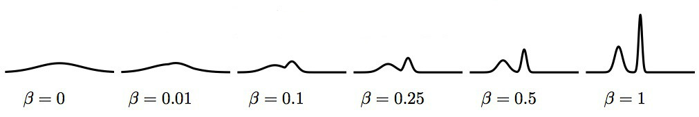
Figure 9: Illustration of constructing the annealed distribution path from the initial distribution $p_{0}({\boldsymbol{x}})$ and the target distribution $p({\boldsymbol{x}})$ in one-dimension case. $p_{\ell}(\boldsymbol{x})\propto p_{0}(\boldsymbol{x})^{1-\beta_{\ell}}p(\boldsymbol{x})^{\beta_{\ell}},$ with $\beta=0,0.01,0.1,0.25,0.5,1.0$, respectively.

Annealed SVGD starts from a set of particle $\{x_{i}^{0}\}_{i=1}^{n}$ drawn from $p_{0}$, and at the $\ell$-th iteration, updates the particles so that $\{x_{i}^{\ell+1}\}_{i=1}^{n}$ approximates the intermediate distribution $p_{\ell+1}$ by running $m$ steps of SVGD with $p_{\ell+1}$ as the target. See Algorithm 6. In practice, $m=1$ is sufficient when $T$ is large.

Algorithm 7 Annealed GF-SVGD (AGF-SVGD)

  Input: Target distribution $p(\boldsymbol{x})$; initial distribution $p_{0}(\boldsymbol{x})$; intermediate distributions $\{p_{t}\}_{t=1}^{T}$.

  Goal: Particles $\{\boldsymbol{x}_{i}\}_{i=1}^{n}$ to approximate $p(\boldsymbol{x}).$

  Initialize particles $\{{\boldsymbol{x}}^{0}_{i}\}_{i=1}^{n}$ drawn from $p_{0}$.

  for iteration $\ell=0,\cdots,T-1$ do

     

$$\boldsymbol{x}_{i}^{\ell+1}\leftarrow\boldsymbol{x}_{i}^{\ell}+\Delta{\boldsymbol{x}}_{i}^{\ell},~{}~{}\forall i=1,\ldots,n,~{}~{}\text{where}~{}$$

$$\!\!\!\!\!\!\!\!\!\!\!\!\!\!\!\!\!\!\!\Delta{\boldsymbol{x}}_{i}^{\ell}=\frac{\epsilon_{\ell,i}}{Z_{\ell}}\sum_{j=1}^{n}w_{j}^{\ell}\big{[}\boldsymbol{s}^{\rho}_{j,\ell+1}k({\boldsymbol{x}}_{j}^{\ell},{\boldsymbol{x}}_{i}^{\ell})+\nabla_{{\boldsymbol{x}}_{j}}k({\boldsymbol{x}}_{j}^{\ell},{\boldsymbol{x}}_{i}^{\ell})\big{]},\vspace{-1em}$$

where $\boldsymbol{s}^{\rho}_{j,\ell+1}=\nabla_{\boldsymbol{x}}\log\rho_{\ell+1}({\boldsymbol{x}}_{j}^{\ell})$ and $\rho_{\ell+1}$ is defined in (0.88); $w_{j}^{\ell}=\rho_{\ell+1}({\boldsymbol{x}}_{j}^{\ell})/p_{\ell+1}({\boldsymbol{x}}_{j}^{\ell})$, $Z_{\ell}=\sum_{j=1}^{n}w_{j}^{\ell}$.

  end for

  Output: $\{\boldsymbol{x}_{i}^{T}\}_{i=1}^{n}$ to approximate $p.$

It is useful to consider the special case when $p_{0}=const$, and hence $p_{\ell}(\boldsymbol{x})\propto p(\boldsymbol{x})^{\alpha_{\ell}}$, yielding an annealed SVGD update of form

$$\Delta{\boldsymbol{x}}_{i}=\frac{\epsilon}{n}\sum_{j=1}^{n}[\nabla_{\boldsymbol{x}}\log p({\boldsymbol{x}}_{j})k({\boldsymbol{x}}_{j},{\boldsymbol{x}}_{i})+\frac{1}{\beta_{\ell}}\nabla_{{\boldsymbol{x}}_{j}}k({\boldsymbol{x}}_{j},{\boldsymbol{x}}_{i})],$$

where the repulsive force is weighted by the inverse temperature $1/\beta_{\ell}$. As $\beta_{\ell}$ increases from 0 to 1, the algorithm starts with a large repulsive force and gradually decreases it to match the temperature of the distribution of interest. This procedure is similar to the typical simulated annealing, but enforces the diversity of the particles using the deterministic repulsive force, instead of random noise.

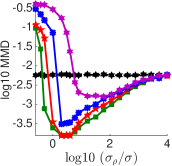
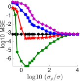
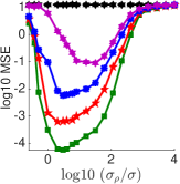
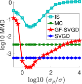
(a) MMD	(b) Mean	(c) Variance		(d) MMD

Figure 10: Results of GF-SVGD on 2D multivariate Gaussian distribution as we change the mean $\boldsymbol{\mu}_{\rho}$ and variance $\sigma_{\rho}$ of the surrogate $\rho({\boldsymbol{x}})$. We can see that the best performance is achieved by matching the mean of $\rho$ and the target $p$ ($\boldsymbol{\mu}_{\rho}=\boldsymbol{\mu}$), and making $\sigma_{\rho}$ slightly larger than the variance $\sigma$ of $p$ (e.g., $\log 10(\sigma_{\rho}/\sigma)\approx 0.5$ or $\sigma_{\rho}\approx 3\sigma$). (d) uses the same setting with $||\boldsymbol{\mu}_{\rho}-\boldsymbol{\mu}||^{2}=8$, but also adds the result of exact Monte Carlo sampling, gradient-based SVGD, and importance sampling (IS) whose proposal is $\rho$, the same as the auxiliary distribution used by GF-SVGD shown in the red curve. We use $n=100$ particles in this plot.

Annealed Gradient-Free SVGD (AGF-SVGD) is the gradient-free version of annealed SVGD which replaces the SVGD update with an GF-SVGD update. Specifically, at the $\ell$-th iteration when we want to update the particles to match $p_{\ell+1}$, we use a GF-SVGD update with auxiliary distribution $\rho_{\ell+1}\approx p_{\ell+1}$, which we construct by using a simple kernel curve estimation

$$\rho_{\ell+1}({\boldsymbol{x}})\propto\sum_{j=1}^{n}p_{\ell+1}({\boldsymbol{x}}_{j}^{\ell})k_{\rho}({\boldsymbol{x}}_{j}^{\ell},{\boldsymbol{x}}),$$ (0.88)

where $k_{\rho}$ is a smoothing kernel (which does not have to be positive definite). Although there are other ways to approximate $p_{\ell+1}$, this simple heuristic is computationally fast, and the usage of smoothing kernel makes $\rho_{\ell+1}$ an over-dispersed estimation which we show perform well in practice (see Figure 10). Note that here $\rho_{\ell+1}$ is constructed to fit smooth curve $p_{\ell+1}$, which leverages the function values of the distribution $p_{\ell+1}({\boldsymbol{x}})$ and is insensitive to the actual distribution of the current particles $\{{\boldsymbol{x}}_{j}^{\ell}\}$. It would be less robust to construct $\rho_{t+1}$ as a density estimator of distribution $p_{\ell+1}$ because the actual distribution of the particles may deviate from what we expect in practice.

The procedure is organized in Algorithm 7. Combining the idea of simulated annealing with gradient-free SVGD makes it easier to construct an initial surrogate distribution and estimate a good auxiliary distribution at each iteration, decreasing the variance of the importance weights. We find that it significantly improves the performance over the basic GF-SVGD for complex target distributions.

Related Works on Gradient-Free Sampling Methods

Almost all gradient-free sampling methods employ some auxiliary (or proposal) distributions that are different, but sufficiently close to the target distribution, followed with some mechanisms to correct the bias introduced by the surrogate distribution. There have been a few number of bias-correction mechanisms underlying most of the gradient-free methods, including importance sampling, rejection sampling and the Metropolis-Hastings rejection trick. The state-of-the-art gradient-free sampling methods are often based on adaptive improvement of the proposals when using these tricks, this includes adaptive importance sampling and rejection sampling (Gilks & Wild, 1992; Cappé et al., 2008; Cotter et al., 2015; Han & Liu, 2017), and adaptive MCMC methods (e.g., Sejdinovic et al., 2014; Strathmann et al., 2015).

Our method is significantly different from these gradient-free sampling algorithms aforementioned in principle, with a number of key advantages. Instead of correcting the bias by either re-weighting or rejecting the samples from the proposal, which unavoidably reduces the effective number of usable particles, our method re-weights the SVGD gradient and steers the update direction of the particles in a way that compensates the discrepancy between the target and surrogate distribution, without directly reducing the effective number of usable particles.

In addition, while the traditional importance sampling and rejection sampling methods require the proposals to be simple enough to draw samples from, our update does not require to draw samples from the surrogate $\rho$. We can set $\rho$ to be arbitrarily complex as long as we can calculate $\rho({\boldsymbol{x}})$ and its gradient. In fact, $\rho({\boldsymbol{x}})$ does not even have to be a normalized probability, sidestepping the difficult problem of calculating the normalization constant.

Empirical Results

We test our proposed algorithms on both synthetic and real-world examples. We start with testing our methods on simple multivariate Gaussian and Gaussian mixture models, developing insights on the optimal choice of the auxiliary distribution.

We then test AGF-SVGD on Gaussian-Bernoulli restricted Boltzmann machine (RBM) and compare it with advanced gradient-free MCMC such as KAMH (Sejdinovic et al., 2014) and KHMC (Strathmann et al., 2015). Finally, we apply our algorithm to Gaussian process classification on real-world datasets.

We use RBF kernel $k(\boldsymbol{x},\boldsymbol{x}^{\prime})=\exp(-\|\boldsymbol{x}-\boldsymbol{x}^{\prime}\|^{2}/h)$ for the updates of our proposed algorithms and the kernel approximation in (0.88); the bandwidth $h$ is taken to be $h{=}\mathrm{med^{2}}/(2\log(n+1))$ where $\mathrm{med}$ is the median of the current $n$ particles. When maximum mean discrepancy (MMD) (Gretton et al., 2012) is applied to evaluate the sample quality, RBF kernel is used and the bandwidth is chosen based on the median distance of the exact samples so that all methods use the same bandwidth for a fair comparison. Adam optimizer (Kingma & Ba, 2015) is applied to our proposed algorithms for accelerating convergence.

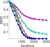
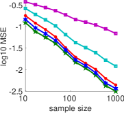
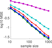
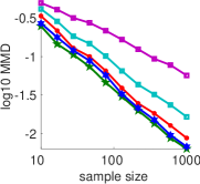
(a) Convergence	(b) Mean	(c) Variance	(d) MMD

Figure 11: Results on GMM with 10 random mixture components and 25 dimensions. (a): the convergence of MMD with fixed sample size of $n=200$. (b)-(c): the MSE vs. sample size when estimating the mean and variance using the particles returned by different algorithms at convergence. (d): the MMD between the particles of different methods and the true distribution $p$. In (b, c, d), 3000 iterations are used. For GF-AIS, the sample size $n$ represents the number of parallel chains, and the performance is evaluated using the weighted average of the particles at the final iteration with their importance weights given by AIS.

Simple Gaussian Distributions

We test our basic GF-SVGD in Algorithm 8 on a simple 2D multivariate Gaussian distribution to develop insights on the optimal choice of $\rho({\boldsymbol{x}})$. We set a Gaussian target $p({\boldsymbol{x}})=\mathcal{N}({\boldsymbol{x}};\boldsymbol{\mu},\sigma I)$ with fixed $\boldsymbol{\mu}=(0,0)$ and $\sigma=2.0$, and an auxiliary distribution $\rho({\boldsymbol{x}})=\mathcal{N}({\boldsymbol{x}};\boldsymbol{\mu}_{\rho},\sigma_{\rho}I)$ where we vary the value of $\boldsymbol{\mu}_{\rho}$ and $\sigma_{\rho}$ in Figure 10. We can see that the best performance is achieved by matching the mean of $\rho$ and the target $p$ ($\boldsymbol{\mu}_{\rho}=\boldsymbol{\mu}$), and making $\sigma_{\rho}$ slightly larger than the variance $\sigma$ of $p$ (e.g., $\log 10(\sigma_{\rho}/\sigma)\approx 0.5$ or $\sigma_{\rho}\approx 3\sigma$). (d) uses the same setting with $||\boldsymbol{\mu}_{\rho}-\boldsymbol{\mu}||^{2}=8$, but also adds the result of exact Monte Carlo sampling, gradient-based SVGD, and importance sampling (IS) whose proposal is $\rho$, the same as the auxiliary distribution used by GF-SVGD shown in the red curve. We use $n=100$ particles in this plot.

The performance is evaluated based on MMD between GF-SVGD particles and the exact samples from $p({\boldsymbol{x}})$ (Figure 10(a)), and the mean square error (MSE) of estimating $\boldsymbol{\mu}$ and $\sigma$ (Figure 10(b)-(c)).

Figure 10 suggests a smaller difference in mean $\boldsymbol{\mu}_{\rho}$ and $\boldsymbol{\mu}$ generally gives better results, but the equal variance $\sigma_{\rho}=\sigma$ does not achieve the best performance. Instead, it seems that $\sigma_{\rho}\approx 3\sigma$ gives the best result in this particular case. This suggests by choosing $\rho$ to be a proper distribution that well covers the probability mass of $p$, it is possible to even outperform the gradient-based SVGD which uses $\rho=p$.

Interestingly, even when we take $\sigma_{\rho}=\infty$, corresponding to the simple update in (0.87) with $\rho=1$, the algorithm still performs reasonably well (although not optimally) in terms of MMD and mean estimation (Figure 10(a)-(b)). It does perform worse on the variance estimation (Figure 10(c)), and we observe that this seems to be because the repulsive force domains when $\sigma_{\rho}$ is large (e.g., when $\sigma_{\rho}=\infty$, only the repulsive term is left as shown in (0.87)), and it causes the particles to be overly diverse, yielding an over-estimation of the variance. This is interesting because we have found that the standard SVGD with RBF kernel tends to underestimate the variance, and a hybrid of them may be developed to give a more calibrated variance estimation.

In Figure 10(d), we add additional comparisons with exact Monte Carlo (MC) which directly draws sample from $p$, and standard importance sampling (IS) with $\rho$ as proposal. We find that GF-SVGD provides much better results than the standard IS strategy with any $\rho$. In addition, GF-SVGD can even outperform the exact MC and the standard SVGD when auxiliary distribution $\rho$ is chosen properly (e.g., $\sigma_{\rho}\approx 3\sigma$). It is interesting to see with proper choice of auxiliary distribution $\rho$ ($\sigma_{\rho}\approx 3\sigma$), GF-SVGD can outperform SVGD in terms of the sample quality.

Comparing GF-SVGD with IS and SVGD

In the following, we compare our GF-SVGD with standard IS and vanilla SVGD on 2-dimensional multivariate Gauss in Fig. 12 and Fig. 13. The target distribution is $p({\boldsymbol{x}})=\mathcal{N}({\boldsymbol{x}};\boldsymbol{\mu},\sigma*I)$, the proposal distribution is $\rho({\boldsymbol{x}})=\mathcal{N}({\boldsymbol{x}};\boldsymbol{\mu}_{0},\sigma_{0}*I)$ and the initial particles of GF-SVGD and SVGD are drawn from $q({\boldsymbol{x}})=\mathcal{N}({\boldsymbol{x}};\boldsymbol{\mu}_{q},\sigma_{q}*I)$ for experiments in Fig. 12 and Fig. 13. We need to calculate the MMD between importance sampler and the target $p.$ We illustrate it in the following. As MMD between $(p_{0},p)$ is

$$\mathrm{MMD}(p_{0},p)=\mathbb{E}_{{\boldsymbol{x}}\sim p_{0},{\boldsymbol{x}}^{\prime}\sim p_{0}}[k({\boldsymbol{x}},{\boldsymbol{x}}^{\prime})]-2\mathbb{E}_{{\boldsymbol{x}}\sim p_{0},{\boldsymbol{y}}\sim p}[k({\boldsymbol{x}},{\boldsymbol{y}})]+\mathbb{E}_{{\boldsymbol{y}}\sim p,{\boldsymbol{y}}^{\prime}\sim p}[k({\boldsymbol{y}},{\boldsymbol{y}}^{\prime})]$$

When we have samples from $q({\boldsymbol{x}})$, we want to calculate MMD between $p_{0}({\boldsymbol{x}})$ and $p({\boldsymbol{x}})$. We can use samples from $q({\boldsymbol{x}})$ and derive a importance weighted MMD,

$$\mathrm{MMD}(p_{0},p) =\mathbb{E}_{{\boldsymbol{x}}\sim q,{\boldsymbol{x}}^{\prime}\sim q}[\frac{p_{0}({\boldsymbol{x}})}{q({\boldsymbol{x}})}k({\boldsymbol{x}},{\boldsymbol{x}}^{\prime})\frac{p_{0}({\boldsymbol{x}}^{\prime})}{q({\boldsymbol{x}}^{\prime})}]$$

$$-2\mathbb{E}_{{\boldsymbol{x}}\sim q,{\boldsymbol{y}}\sim p}[\frac{p_{0}({\boldsymbol{x}})}{q({\boldsymbol{x}})}k({\boldsymbol{x}},{\boldsymbol{y}})]+\mathbb{E}_{{\boldsymbol{y}}\sim p,{\boldsymbol{y}}^{\prime}\sim p}[k({\boldsymbol{y}},{\boldsymbol{y}}^{\prime})].$$

Let ${w({\boldsymbol{x}}_{i})=p_{0}({\boldsymbol{x}}_{i})/p({\boldsymbol{x}}_{i})},\{{\boldsymbol{x}}_{i}\}\sim q({\boldsymbol{x}}),$ $\{{\boldsymbol{y}}_{j}\}_{j=1}^{M}\sim p({\boldsymbol{x}})$ and $\hat{w}({\boldsymbol{x}}_{i})=\frac{w({\boldsymbol{x}}_{i})}{\sum_{i}w({\boldsymbol{x}}_{i})},$ then the importance weighted MMD between $p_{0}({\boldsymbol{x}})$ and $p({\boldsymbol{x}})$ is calculated as follows,

$$\widetilde{\mathrm{MMD}}(p_{0},p)\approx \sum_{i,j}\hat{w}({\boldsymbol{x}}_{i})k({\boldsymbol{x}}_{i},{\boldsymbol{x}}_{j})\hat{w}({\boldsymbol{x}}_{j})$$ (0.89)

$$-\frac{2}{M}\sum_{j=1}^{M}\sum_{i}\hat{w}({\boldsymbol{x}}_{i})k({\boldsymbol{x}}_{i},{\boldsymbol{y}}_{j})+\frac{1}{M^{2}}\sum_{i,j}k({\boldsymbol{y}}_{i},{\boldsymbol{y}}_{j}).$$

As we can see from Fig. 12, under the setting $\|\boldsymbol{\mu}-\boldsymbol{\mu}_{0}\|=2$ and $\sigma_{0}=\sigma=2.0$, GF-SVGD performs much better than IS when IS uses $b$ as importance sampler, the iterations of our GF-SVGD progressively refine the importance proposal (Han & Liu, 2017). It is interesting to observe that our GF-SVGD has almost the same performace as vanilla SVGD except on estimating $\mathbb{E}[{\boldsymbol{x}}]$. The interesting fact that SVGD has very low mean square error (MSE) of estimating $\mathbb{E}[{\boldsymbol{x}}]$ when the target $p$ is Gaussian distribution deserves further investigation.

In Fig.  13, we fix $\|\boldsymbol{\mu}-\boldsymbol{\mu}_{0}\|=2$ and $\sigma=2.0$ and change $\sigma_{0}$. It is interesting to observe that the performance of GF-SVGD increases to certain threshold and then decreases as we increase $\sigma_{0}$. We also empirically check that even when $\sigma_{0}=10^{6}\cdot\sigma$, GF-SVGD still converges to the stationary fixed points but the MSEs of estimating $\mathbb{E}[{\boldsymbol{x}}^{2}]$ and $\mathbb{E}[\cos(\nu{\boldsymbol{x}}+c)]$ are somewhat large. We can see that with proper choice of $\sigma_{0}$, GF-SVGD can further improve the sample efficiency of SVGD in low dimensions in terms of MMD, $\mathbb{E}[{\boldsymbol{x}}^{2}]$ and $\mathbb{E}[\cos(\nu{\boldsymbol{x}}+c)]$ (SVGD already has much better accuracy than the exact Monte Carlo samples). It is also interesting to see that the performance of importance sampling (IS) with importance weight $w({\boldsymbol{x}})=b({\boldsymbol{x}})/p({\boldsymbol{x}})$ also increases first when $\sigma_{0}$ increases to almost the same threshold. Then as when further increases $\sigma_{0}$, the performance of IS also decreases.

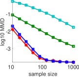
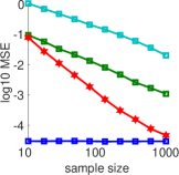
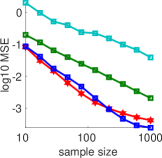
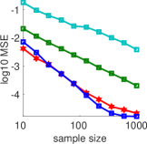
(a) MMD	(b) $E[{\boldsymbol{x}}]$	(c) $E[{\boldsymbol{x}}^{2}]$	(d) $E[\cos(\nu{\boldsymbol{x}}+c)]$

Figure 12: 2D multivariate Gauss distribution. $p({\boldsymbol{x}})=\mathcal{N}(\boldsymbol{\mu},\sigma*I)$, $b({\boldsymbol{x}})=\mathcal{N}(\boldsymbol{\mu}_{0},\sigma_{0}*I)$ and $q({\boldsymbol{x}})=\mathcal{N}(\boldsymbol{\mu}_{q},\sigma_{q}*I)$. $\boldsymbol{\mu}=(0,0)$and $\boldsymbol{\mu}_{0}=(-2,-2)$. $\boldsymbol{\mu}_{q}=(-6,-6).$ Fix $\sigma=\sigma_{0}=\sigma_{q}=2.0$. Monte Carlo (MC) method means samples are directly drawn from $p$ and IS means samples are from $p_{0}$ and applies importance sampling to calculate the corresponding values. The initial particles for GF-SVGD and SVGD are drawn from $q$. We use $T=2000$ for GF-SVGD and SVGD. (a) shows MMD w.r.t. the iterations implemented. (b)-(d) shows MSE for estimating $\mathbb{E}_{p}[h({\boldsymbol{x}})],$ where $h(\boldsymbol{x})=x_{j},~{}x_{j}^{2},~{}\cos(wx_{j}+c)$ with $\nu\sim\mathcal{N}(0,1)$ and $c\in\mathrm{Uniform}(0,1)$ for $j=1,2.$

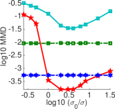
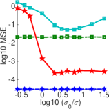
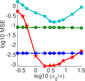
(a) MMD	(b) $E[{\boldsymbol{x}}]$	(c) $E[{\boldsymbol{x}}^{2}]$	(d) $E[\cos(\nu{\boldsymbol{x}}+c)]$

Figure 13: More empirical investigation of the choice of the surrogate distribution in GF-SVGD on 2D multivariate Gaussian distribution. $p({\boldsymbol{x}})=\mathcal{N}(\boldsymbol{\mu},\sigma*I)$, $b({\boldsymbol{x}})=\mathcal{N}(\boldsymbol{\mu}_{0},\sigma_{0}*I)$ and $q({\boldsymbol{x}})=\mathcal{N}(\boldsymbol{\mu}_{q},\sigma_{q}*I)$. $\boldsymbol{\mu}=(0,0)$, $\boldsymbol{\mu}_{0}=(-2,-2)$ and $\boldsymbol{\mu}_{q}=(-6,-6).$ Fix $\sigma=\sigma_{q}=2.0$. Change $\sigma_{0}.$ The number of particles for all methods is 100. The initial particles for both SVGD and GF-SVGD are drawn from distribution $q$. We use $T=2000$ for both GF-SVGD and SVGD. (a) shows MMD w.r.t. the iterations implemented. (b)-(d) shows MSE for estimating $\mathbb{E}_{p}[h({\boldsymbol{x}})],$ where $h(\boldsymbol{x})=x_{j},~{}x_{j}^{2},~{}\cos(wx_{j}+c)$ with $\nu\sim\mathcal{N}(0,1)$ and $c\in\mathrm{Uniform}(0,1)$ for $j=1,2.$

Gaussian Mixture Models (GMM)

We test GF-SVGD and AGF-SVGD on a 25-dimensional GMM with 10 randomly generated mixture components, $p({\boldsymbol{x}})=\frac{1}{10}\sum_{i=1}^{10}\mathcal{N}({\boldsymbol{x}};\boldsymbol{\mu}_{i},I)$, with each element of $\boldsymbol{\mu}_{i}$ is drawn from $\mathrm{Uniform}([-1,1])$. The auxiliary distribution $\rho({\boldsymbol{x}})$ is a multivariate Gaussian $\rho({\boldsymbol{x}})=\mathcal{N}({\boldsymbol{x}};\boldsymbol{\mu}_{\rho},\sigma_{\rho}I)$, with fixed $\sigma_{\rho}=4$ and each element of $\boldsymbol{\mu}_{\rho}$ drawn from $\mathrm{Uniform}([-1,1])$. For AGF-SVGD, we set its initial distribution $p_{0}$ to equal the $\rho$ above in GF-SVGD. Let us now give the description of details for each experiments in Fig. 11. Fig. 11(a) shows the convergence of MMD with fixed sample size of $n=200$. Fig. 11(b) and Fig. 11(c) shows the mean square error with respect to the sample size when estimating the mean and variance using the particles returned by different algorithms at convergence. Fig. 11(d) shows the maximal mean discrepancy(MMD) between the particles of different methods and the true distribution $p$. In Fig. 11(b, c, d), 3000 iterations are used. For comparison, we also tested a gradient-free variant of annealed importance sampling (GF-AIS) (Neal, 2001) with a transition probability constructed by Metropolis-adjusted Langevin dynamics, in which we use the same temperature scheme as our AGF-SVGD, and the same surrogate gradient $\nabla_{{\boldsymbol{x}}}\log\rho_{\ell}$ defined in (0.88). For GF-AIS, the sample size $n$ represents the number of parallel chains, and the performance is evaluated using the weighted average of the particles at the final iteration with their importance weights given by AIS.

Figure 11(a) shows the convergence of MMD vs. the number of iterations of different algorithms with a particle size of $n=200$, and Figure 11(b)-(d) shows the converged performance as the sample size $n$ varies. It is not surprising to see that that standard SVGD converges fastest since it uses the full gradient information of the target $p$. A-SVGD converges slightly slower in the beginning but catches up later; this is because that it uses increasingly more gradient information from $p$. GF-SVGD performs significantly worse, which is expected because it does not leverage the gradient information. However, it is encouraging that annealed GF-SVGD, which also leverages no gradient information, performs much better than GF-SVGD, only slightly worse than the gradient-based SVGD and A-SVGD.

GF-AIS returns a set of particles with importance weights, so we use weighted averages when evaluating the MMD and the mean/variance estimation. This version of GF-AIS is highly comparable to our AGF-SVGD since both of them use the same annealing scheme and surrogate gradient. However, Fig. 11 shows that AGF-SVGD still significantly outperforms GF-AIS.

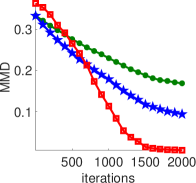
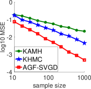
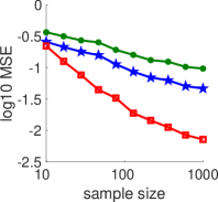
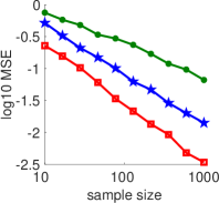
(a) Convergence	(b) Mean	(c) Variance	(d) MMD

Figure 14: Gauss-Bernoulli RBM with $d=20$ and $d^{\prime}=10$. (a): the convergence of MMD with $n=100$ for all the algorithms. The evaluations of MMD of KAMH and KHMC in (a) starts from the burn-in steps of the typical MH algorithm. (b)-(c): the MSE vs. sample size when estimating the mean and variance using the particles returned by different algorithms at 2000 iterations. (d): the MMD between the particles of different algorithms and the true distribution $p$ at 2000 iterations.

Gauss-Bernoulli Restricted Boltzmann Machine

We further compare AGF-SVGD with two recent baselines on Gauss-Bernoulli RBM, defined by

$$p(\boldsymbol{x})\propto\sum_{\boldsymbol{h}}\exp(\boldsymbol{x}^{\top}B\boldsymbol{h}+\boldsymbol{c}_{1}^{\top}\boldsymbol{x}+\boldsymbol{c}_{2}^{\top}\boldsymbol{h}-\frac{1}{2}\|\boldsymbol{x}\|_{2}^{2}),$$ (0.90)

where ${\boldsymbol{x}}\in\mathbb{R}^{d}$ and $\boldsymbol{h}\in\{\pm 1\}^{d^{\prime}}$ is a binary latent variable. By marginalizing the hidden variable $\boldsymbol{h}$, we can see that $p(\boldsymbol{x})$ is a special GMM with $2^{d^{\prime}}$ components. In our experiments, we draw the parameters $\boldsymbol{c}_{1}$ and $\boldsymbol{c}_{2}$ from standard Gaussian and select each element of $B$ randomly from $\{\pm 0.5\}$ with equal probabilities. We set the dimension $d$ of ${\boldsymbol{x}}$ to be 20 and the dimension $d^{\prime}$ of $\boldsymbol{h}$ to be 10 so that $p({\boldsymbol{x}})$ is a 20-dimensional GMM with $2^{10}$ components, for which it is still feasible to draw exact samples by brute-force for the purpose of evaluation. For AGF-SVGD, we set the initial distribution to be $p_{0}({\boldsymbol{x}})=\mathcal{N}({\boldsymbol{x}};\boldsymbol{\mu},\sigma I)$, with $\boldsymbol{\mu}$ drawn from $\mathrm{Uniform}([1,2])$ and $\sigma=3.$

We compare our AGF-SVGD with two recent gradient-free methods: KAMH (Sejdinovic et al., 2014) and KHMC (Strathmann et al., 2015). Both methods are advanced MCMC methods that adaptively improves the transition proposals based on kernel-based approximation from the history of Markov chains. The detailed description of each experiment is provided in the following. Fig. 14(a) shows the convergence of MMD with $n=100$ for all the algorithms. The evaluations of MMD of KAMH and KHMC in (a) starts from the burn-in steps of the typical MH algorithm. Fig. 14(b) and Fig. 14(c) shows the mean square error (MSE) w.r.t the sample size when estimating the mean and variance using the particles returned by different algorithms at 2000 iterations. Fig. 14(d) shows the maximal mean discrepancy (MMD) between the particles of different algorithms and the true distribution $p$ at 2000 iterations.

For a fair comparison with SVGD, we run $n$ parallel chains of KAMH and KHMC and take the last samples of $n$ chains for estimation. In addition, we find that both KAMH and KHMC require a relatively long burn-in phase before the adaptive proposal becomes useful. In our experiments, we use 10,000 burn-in steps for both KAMH and KHMC, and exclude the computation time of burn-in when comparing the convergence speed with GF-SVGD in Figure 14; this gives KAMH and KHMC much advantage for comparison, and the practical computation speed of KAMH and KHMC is much slower than our AGF-SVGD. From Figure 14 (a), we can see that our AGF-SVGD converges fastest to the target $p$, even when we exclude the 10,000 burn-in steps in KAMH and KHMC. Fig. 14 (b, c, d) shows that our AGF-SVGD performs the best in terms of the accuracy of estimating the mean, variance and MMD.

Gaussian Process Classification

We apply our AGF-SVGD to sample hyper-parameters from marginal posteriors of Gaussian process (GP) binary classification. Consider a classification of predicting binary label $y\in\{\pm 1\}$ from feature $\boldsymbol{z}$. We assume $y$ is generated by a latent Gaussian process $f(\boldsymbol{z})$, $p(y|\boldsymbol{z})=1/(1+\exp(-yf(\boldsymbol{z})))$ and $f$ is drawn from a GP prior $f\sim GP(0,k_{f,\boldsymbol{\theta}})$, where $k_{f,\boldsymbol{\theta}}$ is the GP kernel indexed by a hyperparameter $\boldsymbol{\theta}$. In particular, we assume $k_{f,\boldsymbol{\theta}}(\boldsymbol{z},\boldsymbol{z}^{\prime})=\exp(-\frac{1}{2}||(\boldsymbol{z}-\boldsymbol{z}^{\prime})./\exp(\boldsymbol{\theta})||^{2})$, where $./$ denotes the element-wise division and $\boldsymbol{\theta}$ is a vector of the same size as $\boldsymbol{z}$. Given a dataset $Y=\{y_{i}\}$ and $Z=\{\boldsymbol{z}_{i}\}$, we are interested in drawing samples from the posterior distribution $p(\boldsymbol{\theta}|Z,Y)$. Note that the joint posterior of $(\boldsymbol{\theta},f)$ is

$$p(\boldsymbol{\theta},f|Z,Y)=p(Y|f,Z)p(f|\boldsymbol{\theta})p(\boldsymbol{\theta}).$$

Since it is intractable to exactly calculate the marginal posterior of $\boldsymbol{\theta}$, we approximate it by

$$\hat{p}(\boldsymbol{\theta}|Z,Y):=p(\boldsymbol{\theta})\frac{1}{m}\sum_{i=1}^{m}\frac{p(Y|f^{i},Z)p(f^{i}|\boldsymbol{\theta})}{q(f^{i}|\boldsymbol{\theta})},$$ (0.91)

where $\{f^{i}\}_{i=1}^{m}$ is drawn from a proposal distribution $q(f\mid\boldsymbol{\theta})$, which is constructed by an expectation propagation-based approximation of $p(f|\boldsymbol{\theta},Z,Y)$ following Filippone & Girolami (2014).

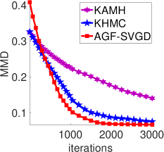
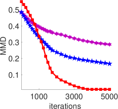
(a) Glass dataset	(b) SUSY dataset

Figure 15: Sampling from the marginal posteriors on GP classification for Glass dataset (a) and SUSY dataset (b). We use a sample size of $n=200$ for all methods.

We run multiple standard Metropolis-Hastings chains to obtain ground truth samples from $p(\boldsymbol{\theta}\mid D)$, following the procedures in section 5.1 of Sejdinovic et al. (2014) and Appendix D.3 of Strathmann et al. (2015). We test the algorithms on Glass dataset and SUSY dataset in Figure 15 from UCI repository (Asuncion & Newman, 2007) for which the dimension of $\boldsymbol{\theta}$ is $d=9$ and $d=18$, respectively. We initialize our algorithm with draws from $p_{0}({\boldsymbol{x}})=\mathcal{N}({\boldsymbol{x}};\boldsymbol{\mu},\sigma I)$ where $\sigma=3$ and each element of $\boldsymbol{\mu}$ is drawn from $\mathrm{Uniform}([-1,1])$. For KAMH and KHMC, we again run $n$ parallel chains and initialize them with an initial burn-in period of 6000 steps which is not taken into account in evaluation. Figure 15 shows that AGF-SVGD again converges faster than KAMH and KHMC, even without the additional burn-in period.

Conclusions and Discussions

We derive a gradient-free extension of Stein’s identity and Stein discrepancy and propose a novel gradient-free sampling algorithm. The $\mathrm{KL}$ divergence between the iterated distribution and the target distribution is maximally decreased with a new kernel $\rho({\boldsymbol{x}})/p({\boldsymbol{x}})k({\boldsymbol{x}},{\boldsymbol{x}}^{\prime})\rho({\boldsymbol{x}}^{\prime})/p({\boldsymbol{x}}^{\prime})$ in RKHS, which is in contrast with the decrease rate of $\mathrm{KL}$ divergence in SVGD with kernel $k({\boldsymbol{x}},{\boldsymbol{x}}^{\prime})$. It is interesting to observe that the gradient-free SVGD performs even better than the original gradient-based SVGD in some experiments with the same number of iterations, where both methods have the same initialization of particles. We expect the reason is that the decrease rate of gradient-free SVGD is even larger than that of gradient-based SVGD in these settings. Future direction includes theoretical investigation of optimal choice of the auxiliary proposal with which we may leverage the gradient of the target to further improve the sample efficiency over the standard SVGD. Our gradient-free sampling framework provides a powerful tool to perform statistical inference on the target distributions whose gradients are unavailable or intractable. The gradient-free kernelized Stein discrepancy we derive can be applied to perform the goodness-of-fit test (Liu et al., 2016) and black-box importance sampling (Liu & Lee, 2017) when the gradients of the target distributions are unavailable or intractable.

Gradient-Free Black-Box Importance Sampling

In the last section of this chapter, we are going to introduce a new algorithm which basically equips any given set of particles $\{{\boldsymbol{x}}_{i}\}_{i=1}^{n}$ with importance weights $\{u_{i}\}_{i=1}^{n}$ so that

$$\sum_{i=1}^{n}u_{i}h(\boldsymbol{x}_{i})\approx\mathbb{E}_{{\boldsymbol{x}}\sim p}[h(\boldsymbol{x})],$$ (0.92)

for general test function $h(\boldsymbol{x})$. In the following, we first discuss the idea of black-box importance sampling (Liu & Lee, 2017), which requires the gradient information of the target distribution $p({\boldsymbol{x}}).$ Then we introduce a gradient-free version of black-box importance sampling, motivated from gradient-free kernelized Stein discrepancy derived in Theorem 5.

Let $k(\boldsymbol{x},\boldsymbol{y})$ be the kernel of the reproducing kernel Hilbert space (RKHS) $\mathcal{H}_{d}.$ Based on the Stein’s identy, it is easy to know the following identity,

$$\mathbb{E}_{\boldsymbol{x}\sim p}[\kappa_{p}(\boldsymbol{x},\boldsymbol{y})]=0,~{}\text{for}~{}\boldsymbol{y}\in\mathcal{X}$$ (0.93)

where the positive definite kernel $\kappa_{p}(\boldsymbol{x},\boldsymbol{y})$ is defined as

$$\kappa_{p}(\boldsymbol{x},\boldsymbol{y})= \boldsymbol{s}_{p}(\boldsymbol{x})^{\top}k(\boldsymbol{x},\boldsymbol{y})\boldsymbol{s}_{p}(\boldsymbol{y})+\boldsymbol{s}_{p}(\boldsymbol{x})^{\top}\nabla_{\boldsymbol{y}}k(\boldsymbol{x},\boldsymbol{y})$$ (0.94)

$$+\boldsymbol{s}_{p}(\boldsymbol{y})^{\top}\nabla_{\boldsymbol{x}}k(\boldsymbol{x},\boldsymbol{y})+\nabla_{\boldsymbol{x}}\cdot(\nabla_{\boldsymbol{y}}k(\boldsymbol{x},\boldsymbol{y})).$$

Replace the expectation $\mathbb{E}_{p}[\cdot]$ in (0.93) with the expectation $\mathbb{E}_{q}[\cdot]$ of a different distribution $q,$ (0.93) will not be zero, which provides a discrepancy measure between $q({\boldsymbol{x}})$ and $p({\boldsymbol{x}}),$

$$\mathbb{S}(q,p)=\mathbb{E}_{\boldsymbol{x},\boldsymbol{y}\sim q}[\kappa_{p}(\boldsymbol{x},\boldsymbol{y})]\geq 0,$$ (0.95)

where the square of KSD $\mathbb{S}(q,p)=0$ if and only if $q({\boldsymbol{x}})$ equals $p({\boldsymbol{x}}).$

Black-Box Importance sampling (BBIS)

Let $\{\boldsymbol{x}_{i}\}_{i=1}^{n}$ be a set of points in $\mathbb{R}^{d}$ and we want to find a set of weights $\{u_{i}\}_{i=1}^{n}$, $u_{i}\in\mathbb{R}$, such that the weighted sample $\{\boldsymbol{x}_{i},u_{i}\}_{i=1}^{n}$ closely approximates the target distribution $p(\boldsymbol{x})$ in the sense that

$$\sum_{i=1}^{n}u_{i}h(\boldsymbol{x}_{i})\approx\mathbb{E}_{{\boldsymbol{x}}\sim p}[h(\boldsymbol{x})],$$ (0.96)

for general test function $h(\boldsymbol{x}).$ For this purpose, we define an empirical version of the KSD in (0.125) to measure the discrepancy between $\{\boldsymbol{x}_{i},u_{i}\}_{i=1}^{n}$ and $p(\boldsymbol{x})$,

$$\mathbb{S}(\{\boldsymbol{x}_{i},u_{i}\},~{}p)=\sum_{i,j=1}^{n}u_{i}u_{j}\kappa_{p}(\boldsymbol{x}_{i},\boldsymbol{x}_{j})=\boldsymbol{u}^{\top}\boldsymbol{K}_{p}\boldsymbol{u},$$ (0.97)

where $\boldsymbol{K}_{p}=\{\kappa_{p}(\boldsymbol{x}_{i},\boldsymbol{x}_{j})\}_{i,j=1}^{n}$ and $\boldsymbol{u}=\{u_{i}\}_{i=1}^{n}$. BBIS solves the problem (0.96) by minimizing the discrepancy $\mathbb{S}(\{\boldsymbol{x}_{i},u_{i}\},~{}p)$,

$$\begin{split}\hat{\boldsymbol{u}}=\operatorname*{arg\,min}_{\boldsymbol{u}}\bigg{\{}\boldsymbol{u}^{\top}\boldsymbol{K}_{p}\boldsymbol{u},~{}~{}s.t.~{}~{}\sum_{i=1}^{n}u_{i}=1,~{}~{}~{}u_{i}\geq 0\bigg{\}}.\end{split}$$ (0.98)

Solving the quadratic programming (0.98) does not require how the particles $\{{\boldsymbol{x}}_{i}\}_{i=1}^{n}$ are generated, and hence gives a black-box importance sampling.

Gradient-Free BBIS

Consider the target distribution

$$p(\boldsymbol{x})\propto\rho(\boldsymbol{x})/w({\boldsymbol{x}}),\quad\boldsymbol{x}\in\mathcal{X},$$

where $\rho(\boldsymbol{x})$ is surrogate distribution with tractable gradient information and $w(\boldsymbol{x})$ is a weight function whose gradient is unavailable or intractable, $w(\boldsymbol{x})=\rho(\boldsymbol{x})/p(\boldsymbol{x}).$ In the following, we are going to derive the gradient-free KSD by directly replacing the kernel $k(\boldsymbol{x},\boldsymbol{y})$ with a distribution-informed kernel $\widetilde{k}(\boldsymbol{x},\boldsymbol{y})=w({\boldsymbol{x}})k(\boldsymbol{x},\boldsymbol{y})w(\boldsymbol{y}).$

Theorem 7.

Replace the kernel $k(\boldsymbol{x},\boldsymbol{y})$ with the kernel $\widetilde{k}(\boldsymbol{x},\boldsymbol{y})=w({\boldsymbol{x}})k(\boldsymbol{x},\boldsymbol{y})w(\boldsymbol{y})$ in RKHS $\mathcal{H}_{d},$ the KSD can be rewritten as follows,

$$\widetilde{\mathbb{S}}(q,p)=\mathbb{E}_{\boldsymbol{x},\boldsymbol{y}\sim q}[\widetilde{\kappa}_{p}(\boldsymbol{x},\boldsymbol{y})]\geq 0,$$ (0.99)

where $\widetilde{\kappa}_{p}(\boldsymbol{x},\boldsymbol{y})$ satisfies $\widetilde{\kappa}_{p}(\boldsymbol{x},\boldsymbol{y})=w(\boldsymbol{x})\kappa_{\rho}(\boldsymbol{x},\boldsymbol{y})w(\boldsymbol{y}),$

$$\kappa_{\rho}(\boldsymbol{x},\boldsymbol{y})= \boldsymbol{s}_{\rho}(\boldsymbol{x})^{\top}k(\boldsymbol{x},\boldsymbol{y})\boldsymbol{s}_{\rho}(\boldsymbol{y})+\boldsymbol{s}_{\rho}(\boldsymbol{x})^{\top}\nabla_{\boldsymbol{y}}k(\boldsymbol{x},\boldsymbol{y})$$

$$+\boldsymbol{s}_{\rho}(\boldsymbol{y})^{\top}\nabla_{\boldsymbol{x}}k(\boldsymbol{x},\boldsymbol{y})+\nabla_{\boldsymbol{x}}\cdot(\nabla_{\boldsymbol{y}}k(\boldsymbol{x},\boldsymbol{y})),$$

which does not require the gradient of the target distribution $p({\boldsymbol{x}}).$

Motivated from Liu & Lee (2017), we can equip any given set of particles $\{{\boldsymbol{x}}_{i}\}_{i=1}^{n}$ with importance weights $\{u_{i}\}_{i=1}^{n}$ so that (0.92) gives a good approximation. $\{u_{i}\}_{i=1}^{n}$ can be evaluated by solving a quadratic programming, which does not require the gradient information of the target distribution $p({\boldsymbol{x}}),$

$$\begin{split}\hat{\boldsymbol{u}}=\operatorname*{arg\,min}_{\boldsymbol{u}}\bigg{\{}\boldsymbol{u}^{\top}\widetilde{\boldsymbol{K}}_{p}\boldsymbol{u},~{}~{}s.t.~{}~{}\sum_{i=1}^{n}u_{i}=1,~{}~{}~{}u_{i}\geq 0\bigg{\}},\end{split}$$ (0.100)

where $\widetilde{\boldsymbol{K}}_{p}=\{w({\boldsymbol{x}}_{i})\widetilde{\kappa}_{\rho}(\boldsymbol{x}_{i},\boldsymbol{x}_{j})w({\boldsymbol{x}}_{j})\}_{i,j=1}^{n}$ and $\boldsymbol{u}=\{u_{i}\}_{i=1}^{n}.$

Lemma 8.

The approximation error (0.92) can be bounded by

$$|\sum_{i=1}^{n}u_{i}h({\boldsymbol{x}}_{i})-\mathbb{E}_{p}[h({\boldsymbol{x}})]|\leq C_{h}\sqrt{\widetilde{\mathbb{S}}(\{{\boldsymbol{x}}_{i},u_{i}\},p)}$$ (0.101)

where $\widetilde{\mathbb{S}}(\{\boldsymbol{x}_{i},u_{i}\},p)=\sum_{i,j=1}^{n}u_{i}w({\boldsymbol{x}}_{i})\kappa_{\rho}(\boldsymbol{x}_{i},\boldsymbol{x}_{j})w({\boldsymbol{x}}_{j})u_{j}$ and $C_{h}=\|h-\mathbb{E}_{p}[h]\|_{\mathcal{H}_{d}},$ which depends on $h({\boldsymbol{x}})$ and $p({\boldsymbol{x}})$ but not on $\{\boldsymbol{x}_{i},u_{i}\}_{i=1}^{n}$.

Lemma 8 provides the approximation error of our proposed method (0.100). Under some mild conditions, the approximation error satisfies $|\sum_{i=1}^{n}u_{i}h({\boldsymbol{x}}_{i})-\mathbb{E}_{p}[h({\boldsymbol{x}})]|=O(n^{-\frac{1}{2}}),$ which indicates that the mean square error converges with rate $n^{-\frac{1}{2}}.$ In practice, we can first run GF-SVGD to get a set of particles $\{{\boldsymbol{x}}_{i}\}_{i=1}^{n}$ to approximate the target distribution $p({\boldsymbol{x}})$ and then run GF-BBIS to further refine the particles $\{{\boldsymbol{x}}_{i}\}_{i=1}^{n}$ with the importance weight $\{u_{i}\}_{i=1}^{n}$ so that $\{\boldsymbol{x}_{i},u_{i}\}_{i=1}^{n}$ provides a better approximation of the integration (0.92).

Alpha-Weighted KSD

In practice, it is also possible to incorporate the gradient information of the target distributions into the kernel of RKHS to improve the performance of black-box importance sampling. Instead of applying kernel $w({\boldsymbol{x}})k({\boldsymbol{x}},{\boldsymbol{x}}^{\prime})w({\boldsymbol{x}}^{\prime}),$ where $w({\boldsymbol{x}})=\rho({\boldsymbol{x}})/p({\boldsymbol{x}}),$ it might be beneficial to use a new kernel

$$\widetilde{k}({\boldsymbol{x}},{\boldsymbol{x}}^{\prime})=p({\boldsymbol{x}})^{\alpha}k({\boldsymbol{x}},{\boldsymbol{x}}^{\prime})p({\boldsymbol{x}}^{\prime})^{\alpha}.$$ (0.102)

Based on this new kerenl, we can a new form of kernelized Stein discrepancy between $q$ and $p$ (alpha-weighted KSD) , whose square is given as $\widetilde{\mathcal{S}}(q,p)=E_{{\boldsymbol{x}},{\boldsymbol{x}}^{\prime}\sim q}[\widetilde{\kappa}_{p}({\boldsymbol{x}},{\boldsymbol{x}}^{\prime})],$ where $\widetilde{\kappa}_{p}({\boldsymbol{x}},{\boldsymbol{x}}^{\prime})$ is defined as

$$\widetilde{\kappa}_{p}(\boldsymbol{x},\boldsymbol{x}^{\prime}) =p(\boldsymbol{x})^{\alpha}p(\boldsymbol{x}^{\prime})^{\alpha}\big{[}(\alpha+1)^{2}\boldsymbol{s}_{p}(\boldsymbol{x})^{\top}k(\boldsymbol{x},\boldsymbol{x}^{\prime})\boldsymbol{s}_{p}(\boldsymbol{y})+(\alpha+1)\boldsymbol{s}_{p}(\boldsymbol{x})^{\top}\nabla_{\boldsymbol{y}}k(\boldsymbol{x},\boldsymbol{x}^{\prime})$$ (0.103)

$$+(\alpha+1)\boldsymbol{s}_{p}(\boldsymbol{x}^{\prime})^{\top}\nabla_{\boldsymbol{x}}k(\boldsymbol{x},\boldsymbol{x}^{\prime})+\nabla_{\boldsymbol{x}^{\prime}}\cdot(\nabla_{\boldsymbol{x}}k(\boldsymbol{x},\boldsymbol{x}^{\prime}))\big{]}.$$

It is interesting to investigate the cases when the BBIS induced from alpha-weighted KSD outperforms the original BBIS Liu & Lee (2017).

Summary

We provide a unified framework to sample from the target distribution whose gradient information is unavailable or intractable. Starting from any set of particles $\{{\boldsymbol{x}}_{i}\}_{i=1}^{n},$ GF-SVGD iteratively transports the particles $\{{\boldsymbol{x}}_{i}\}_{i=1}^{n}$ to approximate the target distribution $p({\boldsymbol{x}}).$ GF-SVGD leverages the gradient of the surrogate distribution $\rho({\boldsymbol{x}})$ and corrects the bias with a form of importance weight $\rho({\boldsymbol{x}})/p({\boldsymbol{x}}).$ The $\mathrm{KL}$ divergence between the distribution of the updated particles $\{{\boldsymbol{x}}_{i}\}_{i=1}^{n}$ and the target distribution $p({\boldsymbol{x}})$ is proven to be maximally decreased in the functional space. The performance of GF-SVGD critically depends on the choice of the surrogate distributions. We empirically investigate the choice of the surrogate distributions and have found that the surrogate distributions which have wide variance tend to perform better. Both theoretical justifications and empirical experiments are provided to demonstrate the effectiveness of our provided gradient-free sampling algorithm. We further improve the gradient-free sampling algorithm, which is motivated from annealed importance sampling, by applying the gradient-free update to the intermediate distribution $p_{\ell}(\boldsymbol{x})$ that interpolate between the initial distribution $p_{0}({\boldsymbol{x}})$ and the target distribution $p({\boldsymbol{x}}).$ The initial particles can be drawn from $p_{0}({\boldsymbol{x}})$. Instead of applying gradient-free update to $p({\boldsymbol{x}}),$ we set the intermediate distribution $p_{\ell}(\boldsymbol{x})$ as the target target and the surrogate distribution is constructed on the fly based on the current particles $\{{\boldsymbol{x}}_{i}^{\ell}\}_{i=1}^{n},$ which approximates $p_{\ell-1}(\boldsymbol{x})$ by our update. Therefore, the importance ratio $\rho({\boldsymbol{x}})/p_{\ell}({\boldsymbol{x}})$ is evaluated between two close distributions, which approximates $p_{\ell-1}({\boldsymbol{x}})/p_{\ell}({\boldsymbol{x}}).$ Empirical experiments demonstrate the improved gradient-free update is robust and can be widely applied to perform gradient-free sampling in various methods with different dimensions. In the end, we provide a gradient-free black-box importance sampling algorithm, which equips any given set of particles $\{{\boldsymbol{x}}_{i}\}_{i=1}^{n}$ with importance weights $\{u_{i}\}_{i=1}^{n}$ so that (0.92) gives a good approximation. The theoretical approximation error is provided.

In the next two chapters, we will leverage the gradient-free SVGD and the gradient-free KSD we develop in this chapter to propose the sampling algorithm and the goodness-of-fit test on discrete distributions. The basic idea is to transform the discrete-valued distributions to the corresponding continuous-valued distributions by a simple form of transformation, which are non-differentiable in finite states. In the next chapter, we apply the gradient-free SVGD to the continuous-valued distributions for sampling and use the inverse transform to get the discrete-valued samples.

Sampling from Discrete Distributions

Discrete probabilistic models provide a powerful framework for capturing complex phenomenons and patterns, such as conducting logic, symbolic reasoning(Holland & Leinhardt, 1981), natural language processing(Johnson et al., 2007) and computer vision(Sutton et al., 2012). However, probabilistic inference of high dimensional discrete distribution is in general NP-hard and requires highly efficient approximate inference tools. Traditionally, approximate inference in discrete models is performed by either Gibbs sampling and Metropolis-Hastings algorithms, or deterministic variational approximation, such as belief propagation, mean field approximation and variable elimination methods (Wainwright et al., 2008; Dechter, 1998). However, both of these two types of algorithms have their own critical weaknesses: Monte Carlo methods provides theoretically consistent sample-based (or particle) approximation, but are typically slow in practice, while deterministic approximation are often much faster in speed, but does not provide progressively better approximation like Monte Carlo methods offers. New methods that integrate the advantages of the two methodologies is a key research challenge; see, for example, (Liu et al., 2015a; Lou et al., 2017; Ahn et al., 2016).

Stein variational gradient descent (SVGD) (Liu & Wang, 2016) has been shown a powerful approach for approximate inference on large scale distributions. However, existing forms of SVGD are designed for continuous-valued distributions and requires the availability and tractability of the gradient information of the target distributions. Gradient-free SVGD leverages the gradient information of a surrogate distribution and corrects the bias with a form of importance weights, which does not require the gradient information of the continuous-valued target distribution. In this chapter, we leverage the power of SVGD for the inference of discrete distributions. Our idea is to transform discrete distributions to piecewise continuous distributions, on which gradient-free SVGD, a variant of SVGD that leverages a differentiable surrogate distribution to sample non-differentialbe continuous distributions, is readily applied to perform inference. To do so, we design a simple yet general framework for transforming discrete distributions to equivalent continuous distributions, which is specially tailored for our purpose, so that we can conveniently and effectively construct the differentiable surrogates needed for GF-SVGD.

Outline

This chapter is organized as follows. We first discuss the background and some discrete distributional sampling baselines. Then we introduce our main algorithm to sample from discrete distribution. We provide empirical experiments on discrete graphical probability models to demonstrate the effectiveness of our proposed algorithm.

Background and Other Discrete Sampling Algorithms

We start with briefly introducing gradient-free SVGD (Han & Liu, 2018), which works for nondifferentiable functions by introducing a differentiable surrogate function. Let $p({\boldsymbol{x}})$ be a differentiable density function supported on $\mathbb{R}^{d}$. The goal of GF-SVGD is to find a set of samples $\{{\boldsymbol{y}}^{i}\}_{i=1}^{n}$ (called “particles”) to approximate $p({\boldsymbol{x}})$ in the sense that

$$\lim_{n\to\infty}\frac{1}{n}\sum_{i=1}^{n}f({\boldsymbol{x}}_{i})=\mathbb{E}_{p}[f({\boldsymbol{x}})],$$

for general test functions $f({\boldsymbol{x}})$ without using the gradient information of the target $p({\boldsymbol{x}})$. Note that when this holds for all bounded continuous functions, the empirical distribution of the particles is called weakly converges to $p({\boldsymbol{x}})$.

GF-SVGD achieves this by starting with a set of initial particles $\{{\boldsymbol{y}}^{i}\}_{i=1}^{n}$, and iteratively updates the particles by

$${\boldsymbol{y}}^{i}\leftarrow{\boldsymbol{y}}^{i}+\epsilon{\boldsymbol{\phi}}^{*}({\boldsymbol{y}}^{i}),~{}~{}~{}~{}\forall i=1,\ldots,n,$$ (0.104)

where $\epsilon$ is a step size, and ${\boldsymbol{\phi}}\colon\mathbb{R}^{d}\to\mathbb{R}^{d}$ is a velocity field chosen to drive the particle distribution closer to the target. Assume the distribution of the particles at the current iteration is $q$, and $q_{[\epsilon{\boldsymbol{\phi}}]}$ is the distribution of the updated particles ${\boldsymbol{y}}^{\prime}={\boldsymbol{y}}+\epsilon{\boldsymbol{\phi}}({\boldsymbol{y}})$. The optimal choice of ${\boldsymbol{\phi}}$ can be framed as the following optimization problem:

$${\boldsymbol{\phi}}^{*}=\operatorname*{arg\,max}_{{\boldsymbol{\phi}}\in\mathcal{F}}\bigg{\{}-\frac{d}{d\epsilon}\mathrm{KL}(q_{[\epsilon{\boldsymbol{\phi}}]}~{}||~{}p)\big{|}_{\epsilon=0}\bigg{\}},$$ (0.105)

where $\mathcal{F}$ is a set of candidate velocity fields, and ${\boldsymbol{\phi}}$ is chosen in $\mathcal{F}$ to maximize the decreasing rate on the KL divergence between the particle distribution and the target.

Gradient-free SVGD

(GF-SVGD) (Han & Liu, 2018) extends SVGD to the setting when the gradient of the target distribution does not exist or is unavailable. The key idea is to replace the gradient of differentiable surrogate distribution $\rho({\boldsymbol{y}})$ whose gradient exists and can be calculated easily, and leverage it for sampling from $p({\boldsymbol{y}})$ using a mechanism similar to importance sampling.

The derivation of GF-SVGD is based on the following key observation,

$$w({\boldsymbol{y}}){\mathcal{A}^{\top}_{\rho}}{\boldsymbol{\phi}}({\boldsymbol{y}})={\mathcal{A}^{\top}_{p}}\big{(}w({\boldsymbol{y}}){\boldsymbol{\phi}}({\boldsymbol{y}})\big{)}.$$ (0.106)

where $w({\boldsymbol{y}})=\rho({\boldsymbol{y}})/p({\boldsymbol{y}}).$ Eq. (0.106) indicates that the Stein operation w.r.t. $p$, which requires the gradient of the target $p$, can be transferred to the Stein operator of a surrogate distribution $\rho$, which does not depends on the gradient of $p$. Based on this observation, GF-SVGD modifies to optimize the following object,

$$\!\!\!\!{\boldsymbol{\phi}}^{*} \!=\operatorname*{arg\,max}_{{\boldsymbol{\phi}}\in\mathcal{F}}\{\mathbb{E}_{q}[{\mathcal{A}^{\top}_{p}}(w(x){\boldsymbol{\phi}}({\boldsymbol{y}}))]\}.$$ (0.107)

Similiar to the derivation in SVGD, the optimization problem (0.107) can be analytically solved; in practice, GF-SVGD derives a gradient-free update as ${\boldsymbol{y}}^{i}\leftarrow{\boldsymbol{y}}^{i}+\frac{\epsilon}{n}\Delta{\boldsymbol{y}}^{i},$ where

$$\!\!\!\!\!\!\Delta{\boldsymbol{y}}^{i}\propto\!\sum_{j=1}^{n}\!w({\boldsymbol{y}}_{j})\big{[}\nabla\log\rho({\boldsymbol{y}}^{j})k({\boldsymbol{y}}^{j},{\boldsymbol{y}}^{i})+\nabla_{{\boldsymbol{y}}^{j}}k({\boldsymbol{y}}^{j},{\boldsymbol{y}}^{i})\big{]},$$ (0.108)

which replaces the true gradient $\nabla\log p$ with a surrogate gradient $\nabla\log\rho$, and then uses an importance weight $w({\boldsymbol{y}}_{j}):=\rho({\boldsymbol{y}}^{j})/p({\boldsymbol{y}}^{j})$ to correct the bias introduced by the surrogate. In practice, the weights $\{{\boldsymbol{y}}_{j}\}_{j=1}^{n}$ might have very large variance when the surrogate $\rho({\boldsymbol{y}})$ is different from the target $p({\boldsymbol{y}}).$ The key ingredient reduces to design an effective surrogate to approximate the target distribution reasonably well so that the variance of $\{{\boldsymbol{y}}_{j}\}_{j=1}^{n}$ is small enough for the convergence of the gradient-free SVGD update. Although it might be challenging to construct a good approximation of the continuous-valued target distributions, it is interesting to observe that it is easy to construct an effective surrogate in dicrete-valued distributions by leveraging their discrete structures.

Han & Liu (2018) observed that GF-SVGD can be viewed as a special case of SVGD with an “importance weighted” kernel,

$$\widetilde{k}({\boldsymbol{y}},{\boldsymbol{y}}^{\prime})=\frac{\rho({\boldsymbol{y}})}{p({\boldsymbol{y}})}k({\boldsymbol{y}},{\boldsymbol{y}}^{\prime})\frac{\rho({\boldsymbol{y}}^{\prime})}{p({\boldsymbol{y}}^{\prime})}.$$

Therefore, GF-SVGD inherits the theorectical justifications of SVGD (Liu, 2017). GF-SVGD is proposed to applied to continuous-valued distributions. The goal of this work is to further develop GF-SVGD into a key inference tool for discrete distributions, by proposing a simple yet powerful method to transform discrete distributions to piecewise continuous distributions, which can be efficiently handled by GF-SVGD with easily constructed surrogate distribution.

However, because SVGD only works for continuous distributions, a key open question is if it is possible to exploit it for more efficient inference of discrete distributions.

We apply our proposed algorithm to a wide range of discrete distributions, Ising models, restricted Boltzmann machines, as well as challenging real-world problems drawn from UAI approximate inference competitions and learning binarized neural networks. We find that our proposed algorithm significantly outperforms traditional inference algorithms for discrete distributions.

In particular, our algorithm is shown to be provide a promising tool for ensemble learn of binarized neural network (BNN) in whichs both weights and activations functions are binarized. Learning BNNs have been shown to be a highly challenging problem, because standard backpropagation can not be applied. We cast the learning BNN as a Bayesian inference problem of drawing a set of samples (which in turns forms an ensemle predictor) of the posterior distribution of weights, and apply our SVGD-based algorithm for efficient inference. We show that our method outperforms other widely-used ensemble method such as bagging and AdaBoost in achieving highest accuracy with the same ensemble size.

Related work Markov chain Monte Carlo (MCMC) is routinely used to generate samples from posterior distributions. Among a variety of MCMC algorithms, Hamiltonian Monte Carlo (HMC) promises a better scalability and has enjoyed wide-ranging successes as one of the most reliable approaches in general settings (Neal et al., 2011; Gelman & Meng, 1998), which are originally targeted for sampling from discrete distributions. However, a fundamental limitation of HMC is the lack of support for discrete parameters. The difficulty of extending HMC from the continuous distribution to the discrete distribution comes from the fact that the construction of HMC proposals relies on a numerical solvers which should satisfy the volume preserving property. The idea of transforming the inference of discrete distributions to continuous distributions have been widely studied, which, however, mostly concentrate on leveraging the power of Hamiltionian Monte Carlo (HMC); see, for example, (Afshar & Domke, 2015; Nishimura et al., 2019; Pakman & Paninski, 2013; Zhang et al., 2012a; Dinh et al., 2017).

Our work is instead motivated by leveraging the power of SVGD, which allows us to derive a novel framework for fast and deterministic sampling of inference discrete distributions. Our framework of transforming discrete distributions to piecewise continuous distribution is similiar to Nishimura et al. (2019), but is more general and tailored for the application of GF-SVGD. Our empirical results show that our method outperforms both traditional algorithms such as Gibbs sampling and discontinuous HMC (Nishimura et al., 2019).

Sampling from Discrete Distribution

This section introduces the main idea of this work, provides a simple yet powerful way for leveraging GF-SVGD as a key inference tool for discrete distributions. This is done by converting discrete distributions to piecewise continuous distributions, which can be efficiently handled by GF-SVGD.

Assume we are interested in sampling from a given discrete distribution $p_{*}({\boldsymbol{z}})$, defined on a finite discrete set $\mathcal{Z}=\{a_{1},\ldots,a_{K}\}$. We may assume each $a_{i}$ is a $d$-dimensional vector of discrete values, so that $\mathcal{Z}$ is a product space. Our idea is to construct a piecewise continuous distribution $p_{c}({\boldsymbol{x}})$ for ${\boldsymbol{x}}\in\mathbb{R}^{d}$, and a map $\Gamma\colon\mathbb{R}^{d}\to\mathcal{Z}$, such that the distribution of ${\boldsymbol{z}}=\Gamma({\boldsymbol{x}})$ is $p_{*}$ when ${\boldsymbol{x}}\sim p_{c}$. In this way, we can apply GF-SVGD on $p_{c}$ to get a set of samples $\{{\boldsymbol{x}}^{i}\}_{i=1}^{n}$ and apply transform ${\boldsymbol{z}}^{i}=\Gamma({\boldsymbol{x}}^{i})$ to get samples $\{{\boldsymbol{z}}^{i}\}$ from $p_{*}({\boldsymbol{z}}).$

Definition 9.

A piecewise continuous distribution $p_{c}({\boldsymbol{x}})$ on $\mathbb{R}^{d}$ and map $\Gamma\colon\mathbb{R}^{d}\to\mathcal{Z}$ is called to form a continuous parameterization of $p_{*}$, if ${\boldsymbol{z}}=\Gamma({\boldsymbol{x}})$ follows $p_{*}({\boldsymbol{z}})$ when $x\sim p_{c}$.

Following this definition, we have the following immediate result.

Proposition 10.

$p_{c}$ and $\Gamma$ form a continuous parameterization of discrete distribution $p_{*}$ on $\mathcal{Z}=\{a_{1},\ldots,a_{K}\}$, iff

$$p_{*}(a_{i})=\int_{\mathbb{R}^{d}}p_{c}({\boldsymbol{x}})\mathbb{I}[a_{i}=\Gamma({\boldsymbol{x}})]d{\boldsymbol{x}},$$ (0.109)

for all $i=1,\ldots,K$. Here $\mathbb{I}(\cdot)$ is the 0/1 indicator function, $\mathbb{I}(t)=0$ iff $t=0$ and $\mathbb{I}(t)=1$ if otherwise.

Algorithm 8 Gradient-free SVGD for Discrete Distributions

  Goal: Approximate a given distribution $p_{*}({\boldsymbol{z}})$ on a finite discrete set $\mathcal{Z}$.

  1) Decide a base distribution $p_{0}({\boldsymbol{x}})$ on $\mathbb{R}^{d}$ (such as Gaussian distribution), and a map $\Gamma\colon\mathbb{R}^{d}\to\mathcal{Z}$ which partitions $p_{0}({\boldsymbol{x}})$ evenly. Construct a piecewise continuous distribution $p_{c}({\boldsymbol{x}})$ by (0.122):

$$p_{c}({\boldsymbol{x}})=p_{0}({\boldsymbol{x}})p_{*}(\Gamma({\boldsymbol{x}})).$$

  2) Construct a differentiable surrogate of $p_{c}({\boldsymbol{x}})$, for example, by $\rho({\boldsymbol{x}})\propto p_{0}({\boldsymbol{x}})\tilde{p}_{*}(\tilde{\Gamma}({\boldsymbol{x}})),$ where $\tilde{p}_{*}$ and $\tilde{\Gamma}$ are smooth approximations of $p_{*}({\boldsymbol{z}})$ and $\Gamma$, respectively.

  3) Run gradient-free SVGD on $p_{c}$ with differentiable surrogate $\rho$: Starting from an initial $\{{\boldsymbol{x}}^{i}\}_{i=1}^{n}$ and repeat

$${\boldsymbol{x}}^{i}\leftarrow{\boldsymbol{x}}^{i}+\epsilon\sum_{j=1}^{n}w_{j}(\nabla\rho({\boldsymbol{x}})k({\boldsymbol{x}}^{j},{\boldsymbol{x}}^{i})+\nabla_{{\boldsymbol{x}}^{j}}k({\boldsymbol{x}}^{j},{\boldsymbol{x}}^{i})).$$

where $w_{j}={\rho({\boldsymbol{x}}^{j})}/{p_{c}({\boldsymbol{x}}^{j})}$, and $k({\boldsymbol{x}},{\boldsymbol{x}}^{\prime})$ is a positive definite kernel.

  4) Calculate ${\boldsymbol{z}}^{i}=\Gamma({\boldsymbol{x}}^{i})$ and output sample $\{{\boldsymbol{z}}^{i}\}_{i=1}^{n}$ for approximating the distribution $p_{*}({\boldsymbol{z}})$.

Given a discrete distribution $p_{*}$, there are many different continuous parameterizations. And exact samples of $p_{c}$ yields exact samples of $p_{*}$ following the definition. For the purpose of approximation, the best continuous parameterization should be constructed so that the continuous distribution $p_{c}$ can be efficiently sampled using continuous inference algorithms, which is gradient-free SVGD in our case.

Here we introduce a simple yet powerful framework for constructing continuous parameterizations, which naturally comes with good differentiable surrogates with which gradient-free SVGD can perform efficiently. Our procedure is also highly general and allows us to construct continuous parameterization for different discrete distributions in an almost automatic fashion.

Our method starts with choosing a simple base distribution $p_{0}({\boldsymbol{x}})$ on $\mathbb{R}^{d}$, which we take to be the Gaussian distribution in most cases, and a map $\Gamma$ that evenly partition $p_{0}$.

Definition 11.

A map $\Gamma\colon\mathcal{Z}\to\mathbb{R}^{d}$ is said to evenly partition $p_{0}$ if we have

$$\int_{\mathbb{R}^{d}}p_{0}({\boldsymbol{x}})\mathbb{I}[a_{i}=\Gamma(x)]d{\boldsymbol{x}}=\frac{1}{K},$$ (0.110)

for $i=1,\ldots K$. Following (0.109), this is equivalent to saying that $p_{0}$ and $\Gamma$ forms a continuous relaxation of the uniform distribution $p_{*}(a_{i})=1/K$.

For simple $p_{0}$ such as standard Gaussian distributions, it is straightforward to construct even partitions using the quantiles of $p_{0}$. For example, in one dimensional case $(d=1)$, we can evenly partition any continuous $p_{0}({\boldsymbol{x}})$, ${\boldsymbol{x}}\in\mathbb{R}$ by

$$\Gamma({\boldsymbol{x}})=a_{i}~{}~{}~{}~{}~{}\text{if ~{}~{} $x\in[\eta_{i-1},~{}~{}\eta_{i})$},$$ (0.111)

where $\eta_{i}$ denotes the $i/K$-th quantile of distribution $p_{0}$. In multi-dimensional cases ($d>1$) and when $p_{0}$ is a product distribution:

$$p_{0}({\boldsymbol{x}})=\prod_{j=1}^{d}p_{0,i}(x_{i}).$$

One can easily show that an even partition can be constructed by concatenating one-dimensional even partitions:

$$\Gamma\left(\begin{bmatrix}x_{1}\\ \vdots\\ x_{d}\end{bmatrix}\right)=\begin{bmatrix}\Gamma_{1}(x_{1})\\ \vdots\\ \Gamma_{d}(x_{d})\end{bmatrix},$$

where $\Gamma_{i}(\cdot)$ an even partition of $p_{0,i}$. A particularly simple case is when ${\boldsymbol{z}}$ are binary vectors, that is, $\mathcal{Z}=\{\pm 1\}^{d}$, in which case $\Gamma({\boldsymbol{x}})=\mathrm{sign}({\boldsymbol{x}})$ evenly partitions any distribution $p_{0}$ that is symmetric around the origin.

Given an even partition of $p_{0}$, we can conveniently construct a continuous parameterization of an arbitrary discrete distribution $p_{*}$ by weighting each bin of the partition with corresponding probability in $p_{*}$, that is, we may construct $p_{c}$ by

$$p_{c}({\boldsymbol{x}})\propto p_{0}({\boldsymbol{x}})p_{*}(\Gamma({\boldsymbol{x}})),$$ (0.112)

where $p_{0}({\boldsymbol{x}})$ is weighted by $p_{*}(\Gamma({\boldsymbol{x}}))$, the probability of the discrete value ${\boldsymbol{z}}=\Gamma({\boldsymbol{x}})$ that ${\boldsymbol{x}}$ maps.

Proposition 12.

Assume $\Gamma$ is an even partition of $p_{0}({\boldsymbol{x}})$, and $p_{c}({\boldsymbol{x}})=Kp_{0}({\boldsymbol{x}})p_{*}(\Gamma({\boldsymbol{x}}))$, where $K$ severs as a normalization constant, then $(p_{c},~{}\Gamma)$ is a continuous parameterization of $p_{*}$.

Proof.

We just need to verify that (0.109) holds.

$$\int p_{c}({\boldsymbol{x}})\mathbb{I}[a_{i}=\Gamma({\boldsymbol{x}})]d{\boldsymbol{x}}$$

$$=K\int p_{0}({\boldsymbol{x}})p_{*}(\Gamma({\boldsymbol{x}}))\mathbb{I}[a_{i}=\Gamma({\boldsymbol{x}})]d{\boldsymbol{x}}$$

$$=K\int p_{0}({\boldsymbol{x}})p_{*}(a_{i})\mathbb{I}[a_{i}=\Gamma({\boldsymbol{x}})]d{\boldsymbol{x}}$$

$$=Kp_{*}(a_{i})\int p_{0}({\boldsymbol{x}})\mathbb{I}[a_{i}=\Gamma({\boldsymbol{x}})]d{\boldsymbol{x}}$$

$$=p_{*}(a_{i}),$$

where the last step follows (0.119). ∎

This provides a simple and general approach for constructing continuous parameterizations of arbitrary discrete distributions. Given such a construction , it is also convenient to construct differentiable surrogate of $p_{c}({\boldsymbol{x}})$ in (0.122) for gradient-free SVGD. To do so, note that the non-differetiable part of $p_{c}$ comes from $p_{*}(\Gamma(x))$, and hence we can construct differentiable surrogate of $p_{c}({\boldsymbol{x}})$ by simply removing $p_{*}(\Gamma(x))$ (so that $\rho=p_{0}$), or approximate it with some smooth approximate of it, based on properties of $p_{*}({\boldsymbol{z}})$ and $\Gamma$. See Algorithm 8 for the summarization of our main procedure. As the piecewise continuous distribution $p_{c}({\boldsymbol{x}})$ has at most $K-1$ points which is non-differentiable, it is expected that the updated particles when applying GF-SVGD will theoretically converge to the target with mild conditions. Let us now illustrate our constructions using examples.

discrete-valued distribution	continuous-valued distribution

Figure 16: Illustrating the constructing of $p_{c}$ (red line) of a three-state distribution $p_{*}$ (green bars). The blue dash line represents the base distribution we use, which is a standard Gaussian distribution.

1D Categorical Distribution

Consider the simple discrete distribution $p_{*}$ show in Figure 16, which takes values in $\{-1,0,1\}$ with probabilities $\{0.25,0.45,0.3\}$, respectively. We take the standard Gaussian distribution (blue dash) as the base distribution $p_{0}$, and obtain a continuous parameterization $p_{c}$ using (0.122), in which $p_{0}(x)$ is weighted by the probabilities of $p_{*}$ in each bin. Note that $p_{c}$ is a piecewise continuous distribution. In this case, we may naturally choose the base distribution $p_{0}$ as the differentiable surrogate function to draw samples from $p_{c}$ when using gradient-free SVGD.

In the following, we will empirically investigate the choices of the transform and provide a simple yet practically powerful transform, which will be demonstrated by a number of probability models in the experimental section.

Investigation of the Choice of Transform

There are many choices of the base function $p_{0}$ and the transform. We empirically investigate the optimal choice of the transform on categorical distribution in Fig. 17. In Fig. 17(b, c, d), the base is chosen as $p_{0}(x)=\sum_{i=1}^{5}p_{i}\mathcal{N}(x;\mu_{i},1.0)$ for different $\boldsymbol{\mu}.$ The base $p_{0}(x)$ in Fig. 17(a) can be seen as $\boldsymbol{\mu}=(0.,0.,0.,0.,0.).$ We observe that with simple Gaussian base in Fig. 17(a), the transformed target is easier to draw samples, compared with the multi-modal target in Fig. 17(c, d), which is empirically believed that Gaussian-like distribution is easier to sample than sampling from multi-modal distributions. This suggests that Gaussian base $p_{0}$ is a simple but powerful choice as its induced transformed target is easy to sample by GF-SVGD. As shown in Fig. 10, even if $\rho({\boldsymbol{x}})=p({\boldsymbol{x}}),$ which reduces to Vanilla SVGD, the update of SVGD is inferior with other choice of $\rho({\boldsymbol{x}}).$ Therefore, it is challenging to find the optimal surrogate as we cannot find a uniform metric to measure the optimality of the surrogate and the transform. Nevertheless, we find a simple yet practical surrogate and transform to perform GF-SVGD on discrete distributions.

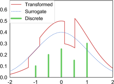
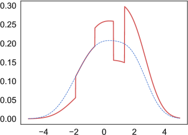
(a), Base $p_{0}(x)=\mathcal{N}(x;0,1)$	(b), $\boldsymbol{\mu}=(-2,-1,0,1,2)$
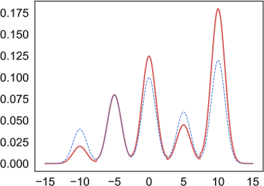
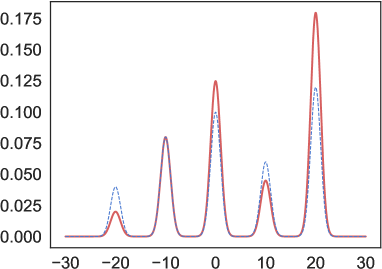
(c), $\boldsymbol{\mu}=(-10,-5,0,5,10)$	(d), $\boldsymbol{\mu}=(-20,-10,0,10,20)$

Figure 17: Illustrating the construction of $p_{c}(x)$ (red line) of a five-state discrete distribution $p_{*}$ (green bars) and the choice of transform. $p_{*}(z)$ takes values $[-2,-1,0,1,2]$ with probabilities $[p_{1},p_{2},p_{3},p_{4},p_{5}]=[0.1,0.2,0.25,0.15,0.3]$ respectively. $K=5.$ The dash blue is the surrogate using base $p_{0}$. Let $p(y)$, $y\in[0,1)$ be the stepwise density, $p(y\in[\frac{i-1}{K},\frac{i}{K}))=p_{i}$, for $i=1,\cdots,K$. In (b, c, d), the base is chosen as $p_{0}(x)=\sum_{i=1}^{5}p_{i}\mathcal{N}(x;\mu_{i},1.)$ and $\boldsymbol{\mu}=(\mu_{1},\mu_{2},\mu_{3},\mu_{4},\mu_{5}).$ The base $p_{0}(x)$ in (a) can be seen as $\boldsymbol{\mu}=(0.,0.,0.,0.,0.).$ Let $F(x)$ be the c.d.f. of $p_{0}(x).$ With variable transform $x=F^{-1}(y)$, the transformed target is $p_{c}(x)=p(F(x))p_{0}(x).$

Binary Ising Models

Consider a binary Ising model of form

$$p_{*}(z)=\exp(b^{\top}z-\frac{1}{2}z^{\top}Az),$$

where $z\in\{\pm 1\}^{d}$ and $b\in\mathbb{R}^{d}$, $A\in\mathbb{R}^{d\times d}$ are the model parameters. We can take the base distribution $p_{0}$ to be any zero-mean Gaussian distribution, e.g., $p_{0}(x)\propto\exp(-\lambda x^{\top}x/2)$, where $x\in\mathbb{R}^{d}$ and $\lambda>0$ is a inverse variance parameter, and take $\Gamma(x)=\mathrm{sign}(x)$, which obviously evenly partition $p_{0}$. Following (0.122), we have

$$p_{c}(x) \propto p_{0}(x)p_{*}(\Gamma(x)),$$

$$\!\!\!\!\!\!\!\!\propto\exp(-\frac{1}{2}\lambda x^{\top}x+b^{\top}\mathrm{sign}(x)-\frac{1}{2}\mathrm{sign}(x)^{\top}A~{}\mathrm{sign}(x)).$$

In this case, it is convenient to construct a differentiable surrogate of $p_{c}$ by simply dropping the $\mathrm{sign}(\cdot)$ function:

$$\rho(x):=\exp(b^{\top}x-\frac{1}{2}x^{\top}(A+\lambda I)x).$$

The $\lambda$ can be properly chosen to match the scale of $A$.

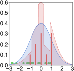
(a) 0th iteration

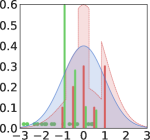
(b) 25th iteration

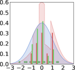
(c) 50th iteration

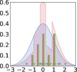
(d) 100th iteration

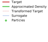
Figure 18: Evolution of real-valued particles $\{x^{i}\}_{i=1}^{n}$ (in green dots) by our discrete sampler in Alg.8 on a one-dimensional categorical distribution. (a-d) shows particles $\{x^{i}\}$ at iteration 0, 10, 50 and 100 respectively. The categorical distribution is defined on states $z\in\{-1,-0.5,0,0.5,1\}$ denoted by $a_{1}$, $a_{2}$, $a_{3}$, $a_{4}$, $a_{5}$, with probabilities $\{0.1,0.2,0.3,0.1,0.3\}$ denoted by $c_{1}$, $c_{2}$, $c_{3}$, $c_{4}$, $c_{5}$, respectively. $p_{*}(z=a_{i})=c_{i}$. The base function is $p_{0}(x)$, shown in blue line. The transformed target to be sampled $p_{c}(x)\propto p_{0}(x)p_{*}(\Gamma(x))$, where $\Gamma(x)=a_{i}$ if $x\in[\eta_{i-1},\eta_{i})$ and $\eta_{i}$ is $i/5$-th quantile of standard Gaussian distribution. The surrogate distribution $\rho(x)$ is chosen as $p_{0}(x)$. We obtain discrete samples $\{z^{i}\}_{i=1}^{n}$ by $z^{i}=\Gamma(x^{i})$.

Empirical Experiments

We apply our algorithm to a number of large scale discrete distributions to demonstrate its empirical effectiveness. We start with illustrating our algorithm on sampling from a simple one-dimensional categorical distribution. We then apply our algorithm to sample from discrete Markov random field, Bernoulli restricted Boltzman machine and models from UAI approximation inference competition. Finally, we apply our method to learn ensemble models of binarized neural networks (BNN).

We use RBF kernel $k(x,x^{\prime})=\exp(-\|x-x^{\prime}\|^{2}/h)$ for the updates of our proposed algorithms; the bandwidth $h$ is taken to be $h{=}\mathrm{med^{2}}/(2\log(n+1))$ where $\mathrm{med}$ is the median of the current $n$ particles. Adam optimizer (Kingma & Ba, 2015) is applied to our proposed algorithms for accelerating convergence.

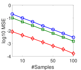
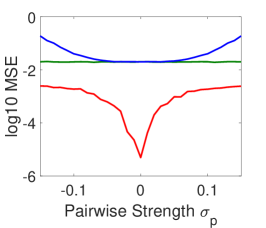
(a) Fixed $\sigma_{p}$	(b) Fixed $n$

Figure 19: Performance of different methods on the Ising model with 10x10 grid. Set $\sigma_{s}=0.01$ in both (a) and (b). We compute the MSE for estimating mean $\mathbb{E}[{\boldsymbol{z}}]$ in each dimension. In (a), we fix $\sigma_{p}=0.1$ and vary the sample size $n$. In (b), we fix the sample size $n=20$ and vary $\sigma_{p}$ from -0.15 to 0.15. In both (a) and (b) we evaluate the $\log\mathrm{MSE}$ based on 200 trails.

Categorical Distribution

We apply our algorithm to sample from one-dimensional categorical distribution $p_{*}(z)$ shown in the red bars in Fig. 18, defined on $\mathcal{Z}:=\{-1,-0.5,0,0.5,1\}$ with corresponding probabilities $\{0.1,0.2,0.3,0.1,0.3\}$. The blue dash line is the surrogate distribution $\rho(y)=p_{0}(x)$, where the base function $p_{0}(x)$ is the p.d.f. of standard Gaussian distribution. The red dash line is the transformed piecewise continuous density $p_{c}(x)\propto p_{0}(x)p_{*}(\Gamma(x))$, where $\Gamma(x)=a_{i}$ if $x\in[\eta_{i-1},\eta_{i})$ and $\eta_{i}$ is $i/5$-th quantile of standard Gaussian distribution. We apply Algorithm 8 to draw a set of samples $\{x^{i}\}_{i=1}^{n}$ (shown in green dots) to approximate the transformed target distribution. Then we can obtain a set of samples $\{z^{i}\}_{i=1}^{n}$ by $z^{i}=\Gamma(x^{i}))$, to get an approximation of the original categorical distribution. As shown in Fig 18, the empirical distribution of the discretized sample $\{z^{i}\}_{i=1}^{n}$ (shown in green bars) aligns closely with the true distribution (the red bars) when the algorithm converges (e.g., at the 100th iteration).

Ising Model

The Ising model (Ising, 1924) is a widely used model in Markov random field. Consider an (undirected) graph $G=(V,E)$, where each vertex $i\in V$ is associated with a binary spin, which consists of ${\boldsymbol{x}}=(x_{1},\cdots,x_{d})$. The probability mass function is $p({\boldsymbol{x}})=\frac{1}{Z}\sum_{(i,j)\in E}\theta_{ij}x_{i}x_{j}$, $x_{i}\in\{-1,1\}$, $\theta_{ij}$ is edge potential and $Z$ is the normalization constant, which is infeasible to calculate when $d$ is high.

As shown in Section 3, it is easy to map $z$ to the piecewise continuous distribution of $x$ in each dimension. We take $\Gamma(x)=\mathrm{sign}(x)$, with the transformed target $p_{c}(x)\propto p_{0}(x)p_{*}(\mathrm{sign}(x))$. The base function $p_{0}(x)$ is taken to be the standard Gaussian distribution on $\mathbb{R}^{d}$. We apply GF-SVGD to sample from $p_{c}(x)$ with the surrogate $\rho(x)=p_{0}(x)$. The initial particles $\{x^{i}\}$ is sampled from $\mathcal{N}(-2,1)$ and update $\{x^{i}\}$ by 500 iterations. We obtain $\{z^{i}\}_{i=1}^{n}$ by $z^{i}=\Gamma(x^{i})$, which approximates the target model $p_{*}(z)$. We compared our algorithm with both Exact Monte Carlo (MC) and Gibbs sampling which is iteratively sampled over each coordinate and use same initialization (in terms of $z=\Gamma(x)$) and number of iterations as ours.

Fig. 19(a) shows the log MSE over the log sample size. With fixed $\sigma_{s}$ and $\sigma_{p}$, our method has the smallest MSE and the MSE has the convergence rate $\mathcal{O}(1/n)$. The correlation $\sigma_{p}$ indicates the difficulty of inference. As $|\sigma_{p}|$ increases, the difficulty increases. As shown in Fig. 19(b), our method can lead to relatively less MSE in the chosen range of correlation. It is interesting to observe that as $\sigma_{p}\rightarrow 0$, our method significantly outperforms MC and Gibbs samplimg.

Algorithm 9 GF-SVGD on training BNN

  Inputs: training set $D$ and testing set $D_{\mathrm{test}}$

  Outputs: classification accuracy on testing set.

  Initialize full-precision models $\{\boldsymbol{W}^{i}\}_{i=1}^{n}$ and its binary form $\{\boldsymbol{W}_{b}^{i}\}_{i=1}^{n}$ where $\boldsymbol{W}^{i}_{b}=\mathrm{sign}(\boldsymbol{W}^{i})$.

  while not converge do

     -Sample $n$ batch data $\{D_{i}\}_{i=1}^{n}.$

     -Calculate the true likelihood $p_{c}(\boldsymbol{W}^{i};D_{i})\propto p_{*}(\mathrm{sign}(\boldsymbol{W}^{i});D_{i})p_{0}(x)$

     -Relax $\boldsymbol{W}^{i}_{b}$ with $\sigma(\boldsymbol{W}^{i})$

     -Relax each sign activation function to the smooth function defined in (0.114) to get $\widetilde{p}$

     -Calculate the surrogate likelihood $\rho(\boldsymbol{W}^{i};D_{i})\propto\widetilde{p}(\sigma(\boldsymbol{W}^{i});D_{i})p_{0}(x)$

     -$\boldsymbol{W}^{i}\leftarrow\boldsymbol{W}^{i}+\Delta\boldsymbol{W}^{i}$, $\forall i=1,\cdots,n,$ where $\Delta\boldsymbol{W}^{i}$ is defined in (0.144).

     -Clip $\{\boldsymbol{W}^{i}\}$ to interval $(-1,1)$ for stability.

  end while

  -Calculate the probability output by softmax layer $p(\boldsymbol{W}^{i}_{b};D_{\mathrm{test}})$

  -Calculate the average probability $f(\boldsymbol{W}_{b};D_{\mathrm{test}})\leftarrow\sum_{i=1}^{n}p(\boldsymbol{W}^{i}_{b};D_{\mathrm{test}})$

  Output test accuracy from $f(\boldsymbol{W}_{b};D_{\mathrm{test}}).$

Bernoulli Restricted Boltzman Machine

Bernoulli restricted Boltzman Machine (RBM) (Hinton, 2002) is an undirected graphical model consisting of a bipartite graph between visible variables ${\boldsymbol{z}}$ and hidden variables $h.$ In a Bernoulli RBM, the joint distribution of visible units ${\boldsymbol{z}}\in\{-1,1\}^{d}$ and hidden units $h\in\{-1,1\}^{M}$ is given by

$$p({\boldsymbol{z}},h)\propto\exp(-E({\boldsymbol{z}},h))$$ (0.113)

where $E({\boldsymbol{z}},h)=-({\boldsymbol{z}}^{\top}Wh+{\boldsymbol{z}}^{\top}b+h^{\top}c)$, $W\in\mathbb{R}^{d\times M}$ is the weight, $b\in\mathbb{R}^{d}$ and $c\in\mathbb{R}^{M}$ are the bias. Marginalizing out the hidden variables $h,$ the probability mass function of ${\boldsymbol{z}}$ is given by $p({\boldsymbol{z}})=\frac{1}{\Omega}\exp(-E({\boldsymbol{z}})),$ with free energy $E({\boldsymbol{z}})=-{\boldsymbol{z}}^{\top}b-\sum_{k}\log(1+\varphi_{k}),$ where $\varphi_{k}=\exp(W_{k*}^{\top}{\boldsymbol{z}}+c_{k})$ and $W_{k*}$ is the k-th row of $W.$

The base function $p_{0}(x)$ is the product of the p.d.f. of the standard Gaussian distribution over the dimension $d.$ Applying the map $z=\Gamma(x)=\mathrm{sign}(x)$, the transformed piecewise continuous target is $p_{c}(x)\propto p_{0}(x)p_{*}(\mathrm{sign}(x)).$ Different from previous example, we construct a simple and more powerful surrogate distrubtion $\rho(x)\propto\widetilde{p}(\sigma({\boldsymbol{y}}))p_{0}(x)$ where $\widetilde{p}(\sigma({\boldsymbol{y}}))$ is differentiable approximation of $p_{*}(x)$ and $\sigma(x)$ is defined as

$$\sigma(x)=\frac{2}{1+\exp(-x)}-1,$$ (0.114)

and $\sigma(x)$ approximates $\mathrm{sign}(x).$ Intuitively, it relaxes the target to a differentiable surrogate with tight approximation, which is plotted in Fig. 20.

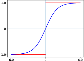
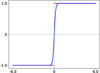
(a), $y=\sigma(x)$	(b), $y=\sigma(10x)$

Figure 20: Illustration the approximation of the relaxation function of $\mathrm{sign}$ function. (b) provides a better approximation than (a) by introducing a temperature parameter.

We compare our algorithm with Gibbis sampling and discontinuous HMC(DMHC, Nishimura et al. (2019)). In Fig. 22, $W$ is drawn from $N(0,0.05)$, both $b$ and $c$ are drawn from $N(0,1).$ With $10^{5}$ iterations of Gibbs sampling, we draw 500 parallel chains to take the last sample of each chain to get 500 ground-truth samples. We run Gibbs, DHMC and GF-SVGD at 500 iterations for fair comparison. In Gibbs sampling, $p({\boldsymbol{z}}\mid h)$ and $p(h\mid{\boldsymbol{z}})$ are iteratively sampled. In DHMC, a coordinate-wise integrator with Laplace momentum is applied to update the discontinuous states. We calculate the maximum mean discrepancy (MMD, Gretton et al. (2012)) between the ground truth sample and the sample drawn by different methods. The kernel used in MMD is the exponentiated Hamming kerenl from Yang et al. (2018), defined as, $k({\boldsymbol{z}},{\boldsymbol{z}}^{\prime})=\exp(-H({\boldsymbol{z}},{\boldsymbol{z}}^{\prime})),$ where $H({\boldsymbol{z}},{\boldsymbol{z}}^{\prime}):=\frac{1}{d}\sum_{i=1}^{d}\mathbb{I}_{\{z_{i}\neq z_{i}^{\prime}\}}$ is normalized Hamming distance. We perform experiments by fixing $d=100$ and varying sample size in Fig. 22(a) and fixing $n=100$ and varying $d$, the dimension of visible units. Fig. 22(a) indicates that the samples from our method match the ground truth samples better in terms of MMD. Fig. 22(b) shows that the performance of our method is least sensitive to the dimension of the model than that of Gibss and DHMC. Both Fig. 22(a) and Fig. 22(b) show that our algorithm converges fastest.

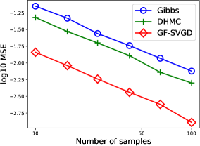
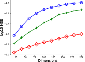
(a) Fix dimension	(b) Fix sample size

Figure 21: Bernoulli RBM with number of visible units $M=25$. In (a), we fix the dimension of visible variables $d=100$ and vary the number of samples $\{{\boldsymbol{z}}^{j}\}_{j=1}^{n}$. In (b), we fix the number of samples $n=100$ and vary the dimension of visible variables $d$. We evaluate the MSE between the estimator and the ground truth quantity.

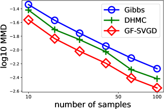
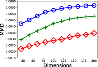
(a) Fix dimension	(b) Fix sample size

Figure 22: Bernoulli RBM with $M=25$. In (a), we fix the dimension of visible variables $d=100$ and vary the number of samples $n$. In (b), we fix $n=100$ and vary $d$. We calculate the MMD between the sample of different methods and the ground-truth sample.

Ensemble Learning on Binarized Neural Networks

We slightly modify our algorithm to the application of training binarized neural network (BNN), where both the weights and activation functions are binary $\pm 1$. BNN has been studied extensively because of its fast computation, energy efficiency and low memory cost (Rastegari et al., 2016; Hubara et al., 2016; Darabi et al., 2018; Zhu et al., 2018). The challenging problem in training BNN is that the gradients of the weights cannot be backpropagated through the binary activation functions because the gradients are zero almost everywhere. Bengio et al. (2013) proposes to use the gradients of identity function, Relu or leaky Relu to approximate the gradients of binary activation functions, which are known as straight-through estimators. While these estimators work well in some cases, their theorectical understanding is largely unexplored although some initial theorectical result in the simple setting has been proposed recently (Yin et al., 2018).

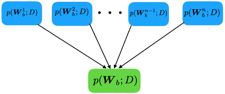
Figure 23: Ensemble learning by drawing n samples $\{p(\boldsymbol{W}^{i}_{b};D)\}_{i=1}^{n}$ from the posterior $p(\boldsymbol{W}_{b};D);$ prediction model $p(\boldsymbol{W}_{b};D)=\frac{1}{n}\sum_{i=1}^{n}p(\boldsymbol{W}^{i}_{b};D).$

We train an ensemble of $n$ neural networks (NN) with the same architecture ($n\geq 2$). Let $\boldsymbol{W}^{i}_{b}$ be the binary weight of model $i$, for $i=1,\cdots,n$, and $p_{*}(\boldsymbol{W}^{i}_{b};D)$ be the target probability model with softmax layer as last layer given the data $D$. Learning the target probability model is framed as drawing $n$ samples $\{\boldsymbol{W}^{i}_{b}\}_{i=1}^{n}$ to approximate the posterior distribution $p_{*}(\boldsymbol{W}_{b};D)$.

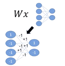
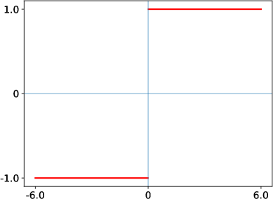
(a), BNN	(b), Activation

Figure 24: Illustration of binarized neural networks(BNN) with binary weights and activation functions.

We apply multi-dimensional quantile transformation ${\boldsymbol{F}}$ to transform the original discrete-valued target to the target distribution of real-valued $\boldsymbol{W}\in\mathbb{R}^{d}$. Let $p_{0}(w)$ be the base function, which is the product of the p.d.f. of the standard Gaussian distribution over the dimension $d.$ Based on the derivation in Section 3, the distribution of $\boldsymbol{W}$ has the form $p_{c}(\boldsymbol{W};D)\propto p_{*}(\mathrm{sign}(\boldsymbol{W});D)p_{0}(\boldsymbol{W})$ with weight $\boldsymbol{W}$ and the $\mathrm{sign}$ function is applied to each dimension of $\boldsymbol{W}$. To backpropagate the gradient to the non-differentiable target, we construct a surrogate probability model $\rho(\boldsymbol{W};D)$ which approximates $\mathrm{sign}(\boldsymbol{W})$ in the transformed target by $\sigma({\boldsymbol{y}})$ and relax the binary activation function $\{-1,1\}$ by $\sigma$, where $\sigma$ is defined by (0.114), denoted by $\widetilde{p}(\sigma(\boldsymbol{W});D)p_{0}(\boldsymbol{W})$. Here $\widetilde{p}(\sigma(\boldsymbol{W});D)$ is a differentiable approximation of $p_{*}(\mathrm{sign}(\boldsymbol{W});D).$ Then we apply GF-SVGD to update $\{\boldsymbol{W}^{i}\}$ to approximate the transformed target distribution of $p_{c}(\boldsymbol{W};D)$ of $\boldsymbol{W}$ as follows, $\boldsymbol{W}^{i}\leftarrow\boldsymbol{W}^{i}+\frac{\epsilon_{i}}{\Omega}\Delta\boldsymbol{W}^{i}$, $\forall i=1,\cdots,n,$

$$\Delta\boldsymbol{W}^{i}\!\!\leftarrow\!\!\!\sum_{j=1}^{n}\!\gamma_{j}[\nabla_{\boldsymbol{W}}\log\rho(\boldsymbol{W}^{j};\!D_{i})k(\boldsymbol{W}^{j}\!,\!\boldsymbol{W}^{i})+\!\nabla_{\boldsymbol{W}^{j}}k(\boldsymbol{W}^{j}\!,\!\boldsymbol{W}^{i})]$$ (0.115)

where $D_{i}$ is batch data and $\mu_{j}=\rho(\boldsymbol{W}^{j};D_{i})/p_{c}(\boldsymbol{W}^{j};D_{i})$, $H(t)\overset{\mathrm{def}}{=}\sum_{j=1}^{n}\mathbb{I}(\mu_{j}\geq t)/n$, $\gamma_{j}=(H(w_{j}))^{-1}$ and $\Omega=\sum_{j=1}^{n}\gamma_{j}$. Note that we don’t need to calculate the cumbersome term $p_{0}(w)$ as it can be canceled from the ratio between the surrogate distribution and the transformed distribution. In practice, we find a more effective way to estimator this density ratio denoted by $\gamma_{j}$. Intuitively, this corresponds to assigning each particle a weight according to the rank of its density ratio in the population. After training the model, we make a prediction on test data $D$ by linearly averaging,

$$p(\boldsymbol{W}_{b};D)=\frac{1}{n}\sum_{i=1}^{n}p(\boldsymbol{W}_{b}^{i};D).$$ (0.116)

Algorithm 9 can be viewed as a new form of the ensemble method for training neural networks models with discrete parameters by drawing a set of samples $\{\boldsymbol{W}_{b}^{i}\}$ from the posterior $p(\boldsymbol{W}_{b};D).$

We test our ensemble algorithm by using AlexNet (Krizhevsky et al., 2012) on CIFAR-10 dataset. We use the same setting for AlexNet as that in Zhu et al. (2018), where the detail can be found in Appendix A. We compare our ensemble algorithm with typical ensemble method using bagging and AdaBoost (BENN, Zhu et al. (2018)), BNN (Hubara et al., 2016) and BNN+(Darabi et al., 2018). Both BNN and BNN+ are trained on a single model with same network structure. From Fig. 25, we can see that all three ensemble methods (GF-SVGD, BAG and BENN) improve test accuracy over one single model (BNN and BNN+). To use the same setting for all methods, we don’t use data augmentation or pre-training. Our ensemble method has the highest accuracy among all three ensemble methods. This is because our ensemble model are sufficiently interactive at each iteration during training and our models $\{\boldsymbol{W}^{i}\}$ in principle are approximating the posterior distribution $p(\boldsymbol{W};D).$

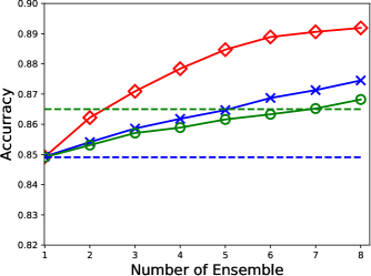
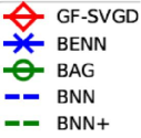
Figure 25: Comparison of different methods using AlexNet with binarized weights and activations on CIFAR10 dataset. We compare our GF-SVGD with BNN (Hubara et al., 2016), BNN+(Darabi et al., 2018) and BENN (Zhu et al., 2018). ”BAG” denote models are independently trained and linearly averaged the softmax output for prediction. Performance is based on the accuracy of different models w.r.t. ensemble size $n$ on test data.

Summary

In this chapter, we propose a new sampling algorithm to sample from the discrete-valued target distributions $p_{*}({\boldsymbol{z}})$. SVGD and GF-SVGD were originally proposed to continuous-valued target distributions. GF-SVGD leverages the gradient information of the surrogate distribution $\rho({\boldsymbol{x}})$ and corrects the bias with a form of importance weights. To exploit GF-SVGD to perform sampling on discrete-valued distributions, we first transform the discrete-valued distributions to the corresponding continuous-valued distributions. We propose a simple yet powerful framework for transforming discrete distributions to equivalent piecewise continuous distribution, on which the differentiable surrogate distribution in GF-SVGD is easy to construct. Our empirical results show that our method consistently outperforms traditional algorithms such as Gibbs sampling and discontinuous Hamiltonian Monte Carlo on various challenging benchmarks of discrete graphical models.

In addition, we demonstrate that our method provides a promising tool for learning an ensemble model of binarized neural network (BNN), outperforming other widely used ensemble methods on learning binarized AlexNet on CIFAR-10 data. We frame learning an ensemble BNN on dataset $D$ as drawing a set of models $\{p(\boldsymbol{W}_{b}^{i};D)\}_{i=1}^{n}$ from the posterior $p(\boldsymbol{W}_{b};D).$ Then to make a prediction on test data, we just linearly average

$$p(\boldsymbol{W}_{b};D)=\sum_{i=1}^{n}p(\boldsymbol{W}_{b}^{i};D).$$

Since $p(\boldsymbol{W}_{b}^{i};D)$ is the softmax layer of the last layer in each neural network and normalized, we just need to sum their probability without introducing 1/n to average them. Our ensemble algorithm is welled justified from the Bayesian perspective. Our ensemble method of learning BNN provides a new way to train BNN. Future research includes applying our ensemble method to training BNN with larger networks such as VGG net and larger dataset such as ImageNet dataset.

In the next chapter, we will leverage our derived gradient-free kernelized Stein discrepancy to perform the goodness-of-fit test on discrete distributions by first transforming the discrete distribution to its continuous counterpart using the transformation constructed in this chapter.

Goodness-of-fit testing on Discrete Distributions

We have introduced two algorithms in Chapter Adaptive Importance Sampling and Chapter Gradient-Free Sampling on Continuous Distributions to perform approximate inference on continuous-valued distributions and one algorithm to sample from discrete-valued distributions Chapter Sampling from Discrete Distributions. The fundamental problem for these three algorithms to tackle is to draw a set of samples $\{{\boldsymbol{x}}_{i}\}_{i=1}^{n}$ to estimate $\mathbb{E}_{p}[f({\boldsymbol{x}})]$ for any interested function $f({\boldsymbol{x}}).$ In this chapter, we will leverage the results in previous chapters to perform a different task, the goodness-of-fit test on discrete distributions. Goodness-of-fit testing measures how well the model $p_{*}({\boldsymbol{z}})$ fits the observed data $\{{\boldsymbol{z}}_{i}\}_{i=1}^{n}$, which is drawn from some unknown distribution $q({\boldsymbol{z}})$. Goodness-of-fit test usually performs null hypothesis $H_{0}:q=p$ versus alternative hypothesis $H_{1}:q\neq p.$ Then gradient-free kernelized Stein discrepancy in Chapter Gradient-Free Sampling on Continuous Distributions can be applied to construct some justified statistics to perform goodness-of-fit testing. The details of our proposed method will be introduced in the following section.

Classical goodness-of-fit tests on discrete distributions includes $\chi^{2}$ test (Pearson, 1900), the Kolmogorov-Smirnov test (Kolmogorov, 1933; Smirnov, 1948) and the Anderson-Darling test (Anderson & Darling, 1954). These tests usually assume the model is fully specified and easy to calculate, which cannot be applied to modern complex models with intractable normalization constants.

Goodness-of-fit testing Algorithm

In this section, we first review gradient-free KSD and then illustrate how it can be leveraged to propose our goodness-of-fit testing algorithm on discrete distributions (Han et al., 2020). As the gradient-free KSD is applied to continuous-valued distributions, we first transform the target distribution $p_{*}({\boldsymbol{z}})$ and the data to a continuous-valued distribution by one-by-one transform. Then we perform the goodness-of-fit test to the transformed data and distribution by naturally choosing gradient-free KSD.

Goodness-of-fit Test on Discrete Distributions

We are given i.i.d. samples $\{{\boldsymbol{z}}_{i}\}_{i=1}^{n}$ from some unknown distribution $q_{*}({\boldsymbol{z}}),$ ${\boldsymbol{z}}\in\{{\boldsymbol{a}}_{1},{\boldsymbol{a}}_{2},\cdots,{\boldsymbol{a}}_{K_{q}}\},$ where $K_{q}$ is the number of discrete states in $q_{*}$, and a candidate discrete distribution $p_{*}({\boldsymbol{z}})$, ${\boldsymbol{z}}\in\{{\boldsymbol{a}}_{1},{\boldsymbol{a}}_{2},\cdots,{\boldsymbol{a}}_{K_{p}}\},$ where $K_{p}$ is the number of discrete states in $p$. $K_{q}$ might not be equal to $K_{p}.$ We would like to measure the goodness-of-fit of the model $p_{*}({\boldsymbol{z}})$ to the observed data $\{{\boldsymbol{z}}_{i}\}_{i=1}^{n}.$ We conduct hypothesis test as follows:

$$\text{null hypothesis}~{}H_{0}:q_{*}=p_{*}~{}\mathrm{vs.}~{}\text{alternative hypothesis}~{}H_{1}:q_{*}\neq p_{*}.$$

Gradient-Free KSD

The gradient-free KSD leverages the gradient information of the surrogate distribution and corrects the bias in KSD (Liu et al., 2016; Gong et al., 2019; Wang et al., 2019) with a form of importance weights. As shown in Theorem 0.99 in Chapter Gradient-Free Sampling on Continuous Distributions, with the choice of kernel $w({\boldsymbol{x}})k({\boldsymbol{x}},{\boldsymbol{x}}^{\prime})w({\boldsymbol{x}}^{\prime})$ in RKHS $\mathcal{H}_{d}$, the square of the gradient-free KSD between $q({\boldsymbol{x}})$ and $p({\boldsymbol{x}})$ is

$$\widetilde{\mathcal{S}}(q,p)=\mathbb{E}_{{\boldsymbol{x}},{\boldsymbol{x}}^{\prime}\sim q}[w({\boldsymbol{x}})k_{\rho}({\boldsymbol{x}},{\boldsymbol{x}}^{\prime})w({\boldsymbol{x}}^{\prime})],$$ (0.117)

where $w({\boldsymbol{x}})=\rho({\boldsymbol{x}})/p({\boldsymbol{x}})$ and $\kappa_{\rho}(\boldsymbol{x},\boldsymbol{x}^{\prime})$ is defined as,

$$\!\!\kappa_{\rho}(\boldsymbol{x},\boldsymbol{x}^{\prime})\!\! =\!\!\boldsymbol{s}_{\rho}(\boldsymbol{x})^{\top}k(\boldsymbol{x},\boldsymbol{x}^{\prime})\boldsymbol{s}_{\rho}(\boldsymbol{x}^{\prime})+\boldsymbol{s}_{\rho}(\boldsymbol{x})^{\top}\nabla_{\boldsymbol{x}^{\prime}}k(\boldsymbol{x},\boldsymbol{x}^{\prime})$$ (0.118)

$$\!\!+\boldsymbol{s}_{\rho}(\boldsymbol{x}^{\prime})^{\top}\nabla_{\boldsymbol{x}}k(\boldsymbol{x},\boldsymbol{x}^{\prime})\!\!+\!\!\nabla_{\boldsymbol{x}}\!\cdot\!(\nabla_{\boldsymbol{x}^{\prime}}k(\boldsymbol{x},\boldsymbol{x}^{\prime})),$$

$\boldsymbol{s}_{\rho}(\boldsymbol{x})$ is the score function of the surrogate distribution $\rho({\boldsymbol{x}}).$ Note that in order to calculate the gradient-free KSD between $q({\boldsymbol{x}})$ and $p({\boldsymbol{x}})$, we only need the evaluation of $p({\boldsymbol{x}})$ and the gradient information of the surrogate distribution $\rho({\boldsymbol{x}})$. The gradient-free KSD can be mapped back to the original KSD by choosing the kernel in (0.197) as $k({\boldsymbol{x}},{\boldsymbol{x}}^{\prime})/(w({\boldsymbol{x}})w({\boldsymbol{x}}^{\prime}))$. Therefore, the gradient-free KSD inherits all theoretical propoerties of the original KSD (Liu et al., 2016) and is a natural choice for goodness-of-fit test.

In order to apply GF-KSD to goodness-of-fit test on discrete distributions, we need to transform the discrete-valued distribution and discrete data to continuous-valued distribution respectively. In the following, let us first review the key steps to transform a discrete-valued distribution to the corresponding continuous-valued distribution. Then we will discuss procedures of transforming discrete data to the corresponding continuous-valued data.

Let $p_{*}({\boldsymbol{z}})$ discrete distribution, defined on a finite discrete set $\mathcal{Z}=\{{\boldsymbol{a}}_{1},\ldots,{\boldsymbol{a}}_{K}\}$. Each ${\boldsymbol{a}}_{i}$ is a $d$-dimensional vector of discrete values. Now we review our idea to construct a piecewise continuous-valued distribution $p_{c}({\boldsymbol{x}})$ for ${\boldsymbol{x}}\in\mathbb{R}^{d}$, and a map $\Gamma\colon\mathbb{R}^{d}\to\mathcal{Z}$, such that the distribution of ${\boldsymbol{z}}=\Gamma({\boldsymbol{x}})$ is $p_{*}$ when ${\boldsymbol{x}}\sim p_{c}$, which has been discussed in Chapter Sampling from Discrete Distributions.

Definition 13.

A piecewise continuous distribution $p_{c}$ on $\mathbb{R}^{d}$ and map $\Gamma\colon\mathbb{R}^{d}\to\mathcal{Z}$ is called to form a continuous parameterization of $p_{*}$, if ${\boldsymbol{z}}=\Gamma({\boldsymbol{x}})$ follows $p_{*}$ when ${\boldsymbol{x}}\sim p_{c}$.

Even Partition

Our method starts with choosing a simple base distribution $p_{0}$, which can be the standard Gaussian distribution. We then construct a map $\Gamma$ that evenly partition $p_{0}$ into several regions with equal probabilities.

Definition 14.

A map $\Gamma\colon\mathcal{Z}\to\mathbb{R}^{d}$ is said to evenly partition $p_{0}$ if we have

$$\int_{\mathbb{R}^{d}}p_{0}({\boldsymbol{x}})\mathbb{I}[{\boldsymbol{a}}_{i}=\Gamma({\boldsymbol{x}})]d{\boldsymbol{x}}=\frac{1}{K},$$ (0.119)

for $i=1,\ldots K$. This is equivalent to saying that $p_{0}$ and $\Gamma$ forms a continuous relaxation of the uniform distribution $q_{*}({\boldsymbol{a}}_{i})=1/K$.

For simple $p_{0}$ such as standard Gaussian distributions, it is straightforward to construct even partitions using the quantiles of $p_{0}({\boldsymbol{x}})$. For example, in the one dimensional case $(d=1)$, we can evenly partition any continuous $p_{0}({\boldsymbol{x}})$, ${\boldsymbol{x}}\in\mathbb{R}$ by

$$\Gamma({\boldsymbol{x}})={\boldsymbol{a}}_{i}~{}~{}~{}~{}~{}\text{if ~{}~{} ${\boldsymbol{x}}\in[\eta_{i-1},~{}~{}\eta_{i})$},$$ (0.120)

where $\eta_{i}$ denotes the $i/K$-th quantile of distribution $p_{0}$. In multi-dimensional cases ($d>1$) and when $p_{0}$ is a product distribution:

$$p_{0}({\boldsymbol{x}})=\prod_{i=1}^{d}p_{0,i}(x_{i}).$$ (0.121)

One can easily show that an even partition can be constructed by concatenating one-dimensional even partition: $\Gamma({\boldsymbol{x}})=(\Gamma_{1}(x_{1}),\cdots,\Gamma_{d}(x_{d})),$ where ${\boldsymbol{x}}=(x_{1},\cdots,x_{d})$ and $\Gamma_{i}(\cdot)$ an even partition of $p_{0,i}$. A particularly simple case is when ${\boldsymbol{z}}$ is a binary vector, i.e., $\mathcal{Z}=\{\pm 1\}^{d}$, in which case $\Gamma({\boldsymbol{x}})=\mathrm{sign}({\boldsymbol{x}})$ evenly partitions any distribution $p_{0}$ that is symmetric around the origin.

Weighting the Partitions

Given an even partition of $p_{0}$, we can conveniently construct a continuous parameterization of an arbitrary discrete distribution $p_{*}$ by weighting each bin of the partition with corresponding probability in $p_{*}$, that is, we may construct $p_{c}({\boldsymbol{x}})$ by

$$p_{c}({\boldsymbol{x}})\propto p_{0}({\boldsymbol{x}})p_{*}(\Gamma({\boldsymbol{x}})),$$ (0.122)

where $p_{0}({\boldsymbol{x}})$ is weighted by $p_{*}(\Gamma({\boldsymbol{x}}))$, the probability of the discrete value ${\boldsymbol{z}}=\Gamma({\boldsymbol{x}})$ that ${\boldsymbol{x}}$ maps.

Definition 15.

The even partition naturally defines a corresponding stepwise distribution $p(\boldsymbol{y})$, $\boldsymbol{y}\in[0,1)^{d},$ as follow: let $F({\boldsymbol{x}})$ is c.d.f. of $p_{0}({\boldsymbol{x}})$ (Gaussian or GMM p.d.f.) in each dimension. If for any $\boldsymbol{y}$, there exists unique ${\boldsymbol{x}}=F^{-1}(\boldsymbol{y})$, ${\boldsymbol{x}}\in[\eta_{i-1},\eta_{i}),$ $p(\boldsymbol{y}):=p_{*}({\boldsymbol{a}}_{i}).$

Derivation of $p_{c}$ from variable transform formula

$p_{c}$ can be derived from the formula of invertible variable transform. The distribution of ${\boldsymbol{x}}$, ${\boldsymbol{x}}=F^{-1}(\boldsymbol{y}),$ is $p(F({\boldsymbol{x}}))\mathrm{det}(F^{\prime}({\boldsymbol{x}}))$, i.e.,

$$p_{c}({\boldsymbol{x}})\!=p(F({\boldsymbol{x}}))\prod_{i=1}^{d}p_{0,i}({\boldsymbol{x}})=p_{0}({\boldsymbol{x}})p(F({\boldsymbol{x}})).$$ (0.123)

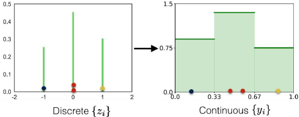
Figure 26: Illustration of transforming the discrete data to continuous data in 1D categorical distribution. The unknown categorical distribution has three states. We correspond each discrete state in the left figure to each unique interval in the right figure. Different colors in left figure means data at different discrete states. Given one sample in left figure, we randomly sample one continuous-valued sample in its corresponding interval in right figure.

Transform Discrete Samples to Continuous Samples

In order to apply continuous-valued GF-KSD, we need to transform samples $\{{\boldsymbol{z}}_{i}\}_{i=1}^{n}$ and the target distribution $p_{*}({\boldsymbol{z}})$ to the corresponding continuous-valued samples and the continuous-valued distribution. In order to do so, Our idea is to transform the testing of discrete distributions $q_{*}=p_{*}$ to their continuous parameterizations. Let $\Gamma$ be a even partition of a base distribution $p_{0}$, and $p_{c}$ and $q_{c}$ are the continuous parameterizations of $p_{*}$ and $q_{*}$ following our construction, respectively, that is,

$$p_{c}({\boldsymbol{x}})\propto p_{0}({\boldsymbol{x}})p_{*}(\Gamma({\boldsymbol{x}})), q_{c}({\boldsymbol{x}})\propto p_{0}({\boldsymbol{x}})q_{*}(\Gamma({\boldsymbol{x}})).$$

Obviously, $p_{c}=q_{c}$ implies that $p_{*}=q_{*}$ (following the definition of continuous parameterization). This allows us to transform the problem to a goodness-of-fit test of continuous distributions, which is achieved by testing if the gradient-free KSD equals zero, $H_{0}:q_{c}=p_{c}$ vs. $H_{1}:q_{c}\neq p_{c}.$

In order to implement our idea, we need to convert the discrete sample $\{{\boldsymbol{z}}_{i}\}_{i=1}^{n}$ from $q_{*}$ to a continuous sample $\{{\boldsymbol{x}}_{i}\}_{i=1}^{n}$ from the corresponding (unknown) continuous distribution $q_{c}$. To achieve this goal, note that when ${\boldsymbol{x}}\sim q_{c}$ and ${\boldsymbol{z}}=\Gamma({\boldsymbol{x}})$, the posterior distribution ${\boldsymbol{x}}$ of giving ${\boldsymbol{z}}={\boldsymbol{a}}_{i}$ equals

$$q({\boldsymbol{x}}~{}|~{}{\boldsymbol{z}}={\boldsymbol{a}}_{i})\propto p_{0}({\boldsymbol{x}})\mathbb{I}(\Gamma({\boldsymbol{x}})={\boldsymbol{a}}_{i}),$$

which corresponds to sampling a truncated version of $p_{0}$ inside the region defined $\{{\boldsymbol{x}}\colon~{}\Gamma({\boldsymbol{x}})={\boldsymbol{a}}_{i}\}$. This can be implemented easily for the simple choices of $p_{0}$ and $\Gamma$. For example, in the case when $p_{0}$ is the product distribution in (0.121) and $\Gamma$ is the concatenation of the quantile-based partition in (0.120), we can sample ${\boldsymbol{x}}~{}|~{}{\boldsymbol{z}}={\boldsymbol{a}}_{i}$ by sample ${\boldsymbol{y}}$ from $\mathrm{Uniform}([\eta_{i-1},\eta_{i})^{d})$ and obtain ${\boldsymbol{x}}$ by ${\boldsymbol{x}}=F^{-1}({\boldsymbol{y}})$ where $F^{-1}$ is the inverse CDF of $p_{0}$.

In the following, we will illustrate the way of transforming the discrete data to continuous data in a number of detailed procedures to make it easier to understand. Let $F$ be the c.d.f. of Gaussian base density $p_{0}.$ Let us first illustrate how to transform one-dimensional samples $\{z_{i}\}_{i=1}^{n}$ to continuous samples.

1. Given discrete data $\{z_{i}\}_{i=1}^{n}.$ Let $\{a_{j}\}_{j=1}^{K}$ are possible discrete states. Assume $K$ is large so that for any $z_{i},$ we have $z_{i}=a_{j}$ for one $j.$

2. For any $z_{i}$ such as $z_{i}=a_{j}$, randomly sample $y_{i}\in[\frac{j-1}{K},\frac{j}{K}).$ We obtain data $\{y_{i}\}_{i=1}^{n}.$

3. Apply $x=F^{-1}(y),$ we obtain data $\{x_{i}\}_{i=1}^{n}.$

Fig. 26 illustrates this procedure in 1D categorical distribution with three states.

For ${\boldsymbol{x}}=(x^{1},\cdots,x^{d}),$ let $F({\boldsymbol{x}})=(F_{1}(x^{1}),\cdots,F_{d}(x^{d})$, where each $F_{i}$ is the c.d.f. of Gaussian density $p_{0,i}(x^{i}).$ We apply the above one-dimensional transform to each dimension of $\{{\boldsymbol{z}}_{i}\}_{i=1}^{n},$ ${\boldsymbol{z}}_{i}=(z_{i}^{1},\cdots,z_{i}^{d}).$ We can easily obtain the continuous data $\{{\boldsymbol{x}}_{i}\}_{i=1}^{n}.$

$$q_{*}({\boldsymbol{z}})\equiv p_{*}({\boldsymbol{z}})~{}\mathrm{iff}~{}q_{c}({\boldsymbol{x}})\equiv p_{c}({\boldsymbol{x}}).$$

Therefore, the problem reduces to perform the hypothesis test$H_{0}:q_{c}=p_{c}$ vs. $H_{1}:q_{c}\neq p_{c}.$

With the one-to-one transform $F^{-1}$ and variable transform formula, the transformed distribution has the form

$$p_{c}({\boldsymbol{x}})=p(F({\boldsymbol{x}}))\prod_{i=1}^{d}F^{\prime}(x^{i}),$$ (0.124)

where ${\boldsymbol{x}}=(x^{1},\cdots,x^{d}).$ Now the original goodness-of-fit test between $q_{*}({\boldsymbol{z}})$ and $p_{*}({\boldsymbol{z}})$ reduces to perform the hypothesis test

$$\text{null hypothesis}~{}H_{0}:q_{c}=p_{c}~{}\mathrm{vs.}~{}\text{alternative hypothesis}~{}H_{1}:q_{c}\neq p_{c}.$$

Let $p_{0}$ be the base function (the product of p.d.f. of Gaussian distribution w.r.t. dimension) and $w({\boldsymbol{x}})=\widetilde{p}_{c}({\boldsymbol{x}})/p_{c}({\boldsymbol{x}})$, $\widetilde{p}_{c}({\boldsymbol{x}})$ is a relaxation of $p_{c}({\boldsymbol{x}})$. With the surrogate $\rho({\boldsymbol{x}})=p_{0}({\boldsymbol{x}})\widetilde{p}(F({\boldsymbol{x}})),$ it is easy to apply the GF-KSD to the transformed discrete distributions between $q_{c}({\boldsymbol{x}})$ and $p_{c}({\boldsymbol{x}})$. The square of GF-KSD between $q_{c}({\boldsymbol{x}})$ and $p_{c}({\boldsymbol{x}})$ has the following form,

$$\widetilde{\mathbb{S}}(q_{c},p_{c})=\mathbb{E}_{\boldsymbol{x},{\boldsymbol{x}}^{\prime}\sim q_{c}}[w(\boldsymbol{x})\kappa_{\rho}(\boldsymbol{x},{\boldsymbol{x}}^{\prime})w({\boldsymbol{x}}^{\prime})],$$ (0.125)

where $\kappa_{\rho}$ is defined in (0.198) with $p_{c}({\boldsymbol{x}})=p_{0}({\boldsymbol{x}})p(F({\boldsymbol{x}}))$ and $\rho({\boldsymbol{x}})=p_{0}({\boldsymbol{x}})\widetilde{p}(F({\boldsymbol{x}})).$

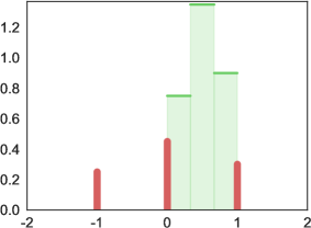
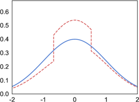
discrete-valued distribution	continuous-valued distribution

Figure 27: Illustrating the construction of $p_{c}({\boldsymbol{x}})$ (red dash line) of a three-state discrete distribution $p_{*}({\boldsymbol{z}})$ (red solid lines). The blue line represents the base distribution $p_{0}({\boldsymbol{x}})$, which is a standard Gaussian distribution.

Let us use the categorical distribution in Fig. 27 to illustrate. The categorical distribution defines on states $z=-1,~{}0,~{}1$ with probability $0.25,~{}0.45,~{}0.3$ respectively, which is shown in red in left figure of Fig. 27. The discrete distribution is bijectively corresponded to a piecewise continuous-valued distribution $p(y)$ (defined within $[0,1]$), which is shown in green in left figure of Fig. 27. The data $\{z_{i}\}_{i=1}^{n}$ can also be transformed to $\{y_{i}\}_{i=1}^{n}.$ By applying the one-to-one transform $F^{-1}$ ($F$ is the c.d.f. of the standard Gaussian distribution), we get the transformed target $p_{c},$ which is shown in dashed red in right figure of Fig.  27. We can choose the surrogate distribution $\rho(x)$ as the p.d.f. of of the standard Gaussian distribution.

Algorithm 10 Goodness-of-fit testing by GF-KSD (GF-KSD)

  Input: Sample $\{{\boldsymbol{z}}_{i}\}_{i=1}^{n}\sim q_{*}$ and its corresponding continuous-valued $\{{\boldsymbol{x}}_{i}\}_{i=1}^{n}\sim q_{c}$, and null distribution $p_{c}$. Base function $p_{0}({\boldsymbol{x}})$ and bootstrap sample size $m$.

  Goal: Test $H_{0}:q=p_{c}$ vs. $H_{1}:q\neq p_{c}$.

  -Compute test statistics $\hat{\mathbb{S}}$ by (0.199).

  -Compute m bootstrap sample $\hat{\mathbb{S}}_{i}^{*}$ by (0.200), $i=1,\cdots,m.$

  -Reject $H_{0}$ with significance level $\alpha$ if the percentage of $\{\hat{\mathbb{S}}^{*}_{i}\}_{i=1}^{m}$ that satisfies $\hat{\mathbb{S}}^{*}>\hat{\mathbb{S}}$ is less than $\alpha.$

With $\{{\boldsymbol{x}}_{i}\}_{i=1}^{n}$ from $q_{c}({\boldsymbol{x}})$, the GF-KSD between $q_{c}({\boldsymbol{x}})$ and $p_{c}({\boldsymbol{x}})$ can be estimated by the U-statistics,

$$\hat{\mathbb{S}}(q_{c},p_{c})=\frac{1}{(n-1)n}\sum_{1\leq i\neq j\leq n}w({\boldsymbol{x}}_{i})\kappa_{\rho}(\boldsymbol{x}_{i},{\boldsymbol{x}}_{j})w({\boldsymbol{x}}_{j})$$ (0.126)

Lemma 16.

Let $k({\boldsymbol{x}},{\boldsymbol{x}}^{\prime})$ be a positive definite kernel. Suppose $\|p({\boldsymbol{x}})(s_{q}({\boldsymbol{x}})-s_{\rho}({\boldsymbol{x}}))\|_{2}^{2}<\infty,$ and $\widetilde{\mathcal{S}}(q,p)=\mathbb{E}_{{\boldsymbol{x}},{\boldsymbol{x}}^{\prime}\sim q}[w({\boldsymbol{x}})k_{\rho}({\boldsymbol{x}},{\boldsymbol{x}}^{\prime})w({\boldsymbol{x}}^{\prime})]<\infty,$ we have:

1. If $q\neq p,$ then $\sqrt{n}(\hat{\mathbb{S}}(q,p)-\mathbb{S}(q,p))\rightarrow\mathcal{N}(0,\sigma_{u}^{2})$ in distribution with the variance $\sigma_{u}^{2}=\mathrm{var}_{{\boldsymbol{x}}\sim q}(\mathbb{E}_{{\boldsymbol{x}}^{\prime}\sim}[w({\boldsymbol{x}})k_{\rho}({\boldsymbol{x}},{\boldsymbol{x}}^{\prime})w({\boldsymbol{x}}^{\prime})]),$ and $\sigma_{u}^{2}\neq 0.$

2. If $q=p,$ then $\sigma_{u}^{2}=0.$ And we have

   $$n\hat{\mathbb{S}}(q,p)\rightarrow\sum_{j=1}^{\infty}c_{j}(Z_{j}^{2}-1),~{}\text{in distribution,}$$

   where $\{Z_{j}\}$ are i.i.d. standard Gaussian random variable, and $\{c_{j}\}$ are the eigenvalues of kernel $w({\boldsymbol{x}})k_{\rho}({\boldsymbol{x}},{\boldsymbol{x}}^{\prime})w({\boldsymbol{x}}^{\prime})$ under distribution $p.$

Proof: The detailed explanation and proof can be found on the appendix LABEL:append:go.

Bootstrap Sample The asymptotic distribution of $\hat{\mathbb{S}}(q_{c},p_{c})$ under the null hypothesis cannot be evaluated. In order to perform goodness-of-fit test, we draw random multinomial weights $u_{1},\cdots,u_{n}\sim\mathrm{Multi}(n;1/n,\cdots,1/n),$ and calculate

$$\hat{\mathbb{S}}^{*}(q_{c},p_{c})=\sum_{i\neq j}(u_{i}\!-\!\frac{1}{n})w({\boldsymbol{x}}_{i})\kappa_{\rho}(\boldsymbol{x}_{i},{\boldsymbol{x}}_{j})w({\boldsymbol{x}}_{j})(u_{j}-\frac{1}{n}).$$ (0.127)

We repeat this process by $m$ times and calculate the critical values of the test by taking the $(1-\alpha)$-th quantile, denoted by $\gamma_{1-\alpha}$, of the bootstrapped statistics $\{\hat{\mathbb{S}}_{i}^{*}(q_{c},p_{c})\}.$

Proposition 17.

Suppose the conditions in 16 hold. For any fixed $q_{c}\neq p_{c},$ the limiting power of the test that rejects the null hypothesis $q_{c}\neq p_{c}$ when $\hat{\mathbb{S}}^{*}(q_{c},p_{c})\geq\gamma_{1-\alpha}$ is one, which means the test is consistent in power against any fixed $q_{c}\neq p_{c}.$

The proof is similar to the procedure in Proposition 4.2 Liu et al. (2016). The Proposition 31 theoretically justifies the correctness of our proposed goodness-of-fit testing algorithm. The whole procedure is summarized in Alg. 10.

Empirical Results

In this section, we conduct some empirical experiments to demonstrate the effectiveness of our proposed goodness-of-fit testing algorithm and compare with two baselines, discrete kernelized Stein discrepancy (Yang et al. (2018), DKSD) and maximum mean discrepancy(Gretton et al. (2012), MMD). We provide numerical comparison of the goodness-of-fit test with baselines on binary Ising model and then Bernoulli restricted Boltzmann machine (RBM) to demonstrate the effectiveness of our proposed algorithm. The performance of all algorithms are based on type-II error rate (false negative rate).

Binary Ising Model

The Ising model (Ising, 1924) is a widely used model in Markov random field. Consider an (undirected) graph $G=(V,E)$, where each vertex $i\in V$ is associated with a binary spin, which consists of ${\boldsymbol{x}}=(x_{1},\cdots,x_{d})$. The probability mass function is $p({\boldsymbol{x}})=\frac{1}{Z}\sum_{(i,j)\in E}\theta_{ij}x_{i}x_{j}$, $x_{i}\in\{-1,1\}$, $\theta_{ij}$ is edge potential and $Z$ is the normalization constant, which is infeasible to calculate when $d$ is high.

In Fig. 28(a, b), $p_{*}$ and $q_{*}$ has temperature $T$ and $T^{\prime}$ respectively. In (a) we vary the parameters $T^{\prime}$ of $q_{*}$ and fix the parameter $T$ of $p_{*}$. Fig. 28(a) shows that when the difference between $T$ and $T^{\prime}$ are in some range $[\alpha,\beta]$, $\alpha>0,\beta>0$, our method has lower False negative rate than DKSD (Yang et al., 2018). When $\alpha$ go to zeros, all methods have the same high error rate. When $\beta$ increases, the performance difference between ours and DKSD is small. In all settings, the MMD always keep perform worst, which indicates that MMD is not a goodness-of-fit test algorithm for such discrete probability models. We fix the models $p_{*}$ and $q_{*}$ and vary the sample size $n$ in (b). We test $H_{0}:q_{*}=p_{*}$ vs. $H_{1}:q_{*}\neq p_{*}.$ MMD keeps performing worst. When the sample size is small, our GF-KSD performs better than DKSD, which indicates that our GF-KSD is more sample-efficient. As the sample size increases, the gap between our GF-KSD and DKSD becomes smaller and smaller.

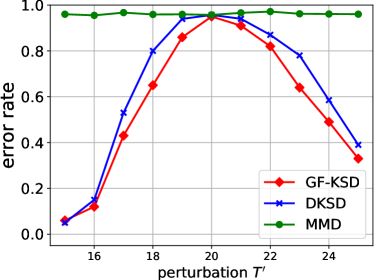
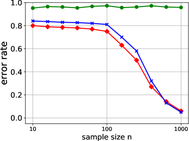
(a) $T=20$ (n=1000)	(b) $T=20$ and $T^{\prime}=15$

Figure 28: Goodness-of-fit testing on Ising model with significant level $\alpha=0.05$. In (a, b), $p_{*}$ and $q_{*}$ has temperature $T$ and $T^{\prime}$ respectively. In (a) we vary the parameters of $q_{*}$. We fix the models and vary the sample size $n$ in (b). We test $H_{0}:q_{*}=p_{*}$ vs. $H_{1}:q_{*}\neq p_{*}.$

Bernoulli restricted Boltzmann Machine

Bernoulli RBM(Hinton, 2002) is an undirected graphical model consisting of a bipartite graph between visible variables ${\boldsymbol{z}}$ and hidden variables ${\boldsymbol{h}}.$ In a Bernoulli RBM, the joint distribution of visible units ${\boldsymbol{z}}\in\{-1,1\}^{d}$ and hidden units $h\in\{-1,1\}^{M}$ is given by

$$p({\boldsymbol{z}},{\boldsymbol{h}})\propto\exp(-E({\boldsymbol{z}},{\boldsymbol{h}}))$$ (0.128)

where $E({\boldsymbol{z}},{\boldsymbol{h}})=-({\boldsymbol{z}}^{\top}W{\boldsymbol{h}}+{\boldsymbol{z}}^{\top}b+{\boldsymbol{h}}^{\top}c)$, $W\in\mathbb{R}^{d\times M}$ is the weight, $b\in\mathbb{R}^{d}$ and $c\in\mathbb{R}^{M}$ are the bias. Marginalizing out the hidden variables ${\boldsymbol{h}},$ the probability mass function of ${\boldsymbol{z}}$ is given by $p({\boldsymbol{z}})\propto\exp(-E({\boldsymbol{z}})),$ with free energy $E({\boldsymbol{z}})=-{\boldsymbol{z}}^{\top}b-\sum_{k}\log(1+\varphi_{k}),$ where $\varphi_{k}=\exp(W_{k*}^{\top}{\boldsymbol{z}}+c_{k})$ and $W_{k*}$ is the k-th row of $W.$

We perform the goodness-of-fit tests on Bernoulli RBM in Fig. 28, which shows the false negative error. In Fig. 29(a, b), $p_{*}$ has $W\sim\mathcal{N}(0,1/M)$ and $q_{*}$ has $W+\epsilon$, where $\epsilon\sim\mathcal{N}(0,\sigma^{\prime}).$ $b$ and $c$ in $p_{*}$ and $q_{*}$ are the same. In Fig. 29(a) we vary the parameters of $q_{*}$. We fix the models and vary the sample size $n$ in Fig. 29(b). Fig. 29(a) shows that as $\sigma^{\prime}$ increases, our GF-KSD performs bettern than DKSD. When $\sigma^{\prime}$ is close to zero ($p_{*}$ and $q_{*}$ are almost the same), the type-II error rate is high, which is expected. In Fig. 29(b), our GF-KSD performs better than DKSD when the sample size $n$ is small. As the sample size $n$ increases, the gap between ours and DKSD becomes smaller and smaller. In all cases, MMD performs the worst.

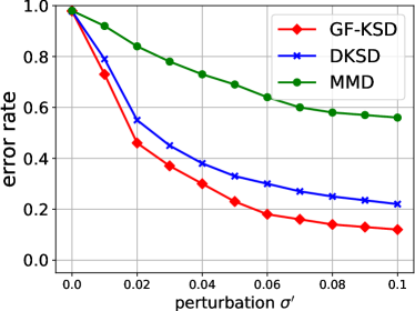
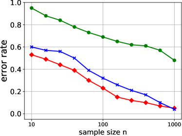
(a) $\sigma=0$ (n=100)	(b) $\sigma=0$ and $\sigma^{\prime}=15$

Figure 29: Goodness-of-fit testing on Bernoulli RBM (a, b) with significant level $\alpha=0.05$. In (a, b), $p_{*}$ has $W\sim\mathcal{N}(0,1/M)$ and $q_{*}$ has $W+\epsilon$, where $\epsilon\sim\mathcal{N}(0,\sigma^{\prime}).$ $b$ and $c$ in $p_{*}$ and $q_{*}$ are the same. In (a) we vary the parameters of $q_{*}$. We fix the models and vary the sample size $n$ in (b).

Summary

In this chapter, we propose an efficient algorithm to perform goodness-of-fit tests on discrete distributions. Our method leverages the gradient information of a surrogate distribution and corrects the bias with a form of importance weight to compute the gradient-free KSD for goodness-of-fit tests. The surrogate distribution can be constructed in an arbitrary form. On discrete distributions, the surrogate distributions can be easily constructed by exploiting the structure of the discrete distributions with simple smoothness trick. It is interesting to theoretically investigate the effective choice of the surrogate distributions. We verify the effectiveness of our proposed algorithm on two widely-used discrete graphical models, binary Ising model and Bernoulli restricted Boltzmann machine. Our proposed algorithm provides a new perspective to perform goodness-of-fit tests on discrete distributions. We expect our algorithm can be widely applied to goodness-of-fit tests on discrete distributions.

Up to the current chapter, we have introduced four efficient approximate inference algorithms and one goodness-of-fit testing method. The non-parametric importance sampling algorithm adaptively improves the importance proposal, which leverages the gradient information of the target distribution. In Chapter Gradient-Free Sampling on Continuous Distributions, we propose gradient-free SVGD, which doesn’t require the gradient information of the target distribution. The $\mathrm{KL}$ divergence between the distribution of the updated particles and the target distribution is maximally decreased in a functional space. We propose gradient-free black-box importance sampling, which equips a set of samples with importance weights so that $\sum_{i=1}^{n}w({\boldsymbol{x}}_{i})h({\boldsymbol{x}}_{i})$ can be applied to estimate $\mathbb{E}_{{\boldsymbol{x}}\sim p}[h({\boldsymbol{x}})].$ In Chapter Sampling from Discrete Distributions, we propose a new algorithm to sample from discrete distributions, which leverages the gradient-free SVGD to sample from the corresponding piecewise continuous-valued target distributions of the discrete distributions.

We have finished all approximate inference algorithms. In the next chapter, we will leverage some widely used approximate inference tools to perform some applications. We will provide one example in distributed learning, where we will We propose an importance-weighted estimator to reduce the variance in bootstrapped samples to estimate one integral when we try to find a global model, which has a minimal sum of $\mathrm{KL}$ divergence with each local model.

Distributed Model Aggregation by Pseudo Importance Sampling

We have introduced two sample-efficient approximate inference algorithms on continuous distributions to estimate $\mathbb{E}_{{\boldsymbol{x}}\sim p}[f({\boldsymbol{x}})]$ with the gradient and without the gradient of the target distribution $p({\boldsymbol{x}})$. We have also introduced one sampling algorithm on discrete distributions. The fundamental problem we have been solving is to find an efficient set of samples $\{{\boldsymbol{x}}_{i}\}_{i=1}^{n}$ to estimate the integration $\mathbb{E}_{{\boldsymbol{x}}\sim p}[f({\boldsymbol{x}})].$ In this chapter, we provide an application in distributed model aggregation, where the setting is slightly different from that of the approximate inference. In the following, we will briefly illustrate the problem we are going to solve in this chapter and provide an algorithm whose key idea is motivated from the tools widely used in approximate inference.

In distributed, or privacy-preserving learning, we are often given a set of probabilistic models estimated from different local repositories $\{p(\boldsymbol{x}|\boldsymbol{\hat{\theta}}_{k})\}_{k=1}^{d}$, where $d$ is the number of local machines and $\boldsymbol{\hat{\theta}}_{k}$ is the parameter of the probabilistic local model, and asked to combine them into a single model $p(\boldsymbol{x}|\boldsymbol{\hat{\theta}})$ that gives efficient statistical estimation. We focuses on a one-shot approach for distributed learning, in which we first learn a set of local models $\{p(\boldsymbol{x}|\boldsymbol{\hat{\theta}}_{k})\}_{k=1}^{d}$ from local machines, and then combine them in a fusion center to form a single model that integrates all the information in the local models. This approach is highly efficient in both computation and communication costs, but casts a challenge problem in designing statistically efficient combination strategies. A simple method is to linearly average the parameters of the local models, $\boldsymbol{\hat{\theta}}=\frac{1}{d}\sum_{j=1}^{d}\boldsymbol{\hat{\theta}}_{j}$. Many studies have been focused on a simple linear averaging method that linearly averages the parameters of the local models (e.g., Zhang et al., 2012b, 2013; Liu et al., 2015c; Rosenblatt & Nadler, 2014; Connamacher et al., 2020; Liu & Ray, 2017; Liu et al., 2019). Although nearly optimal asymptotic error rates can be achieved, this simple method tends to degenerate in practical scenarios for models with non-convex log-likelihood or non-identifiable parameters (such as latent variable models and neural models), and is not applicable at all for models with non-additive parameters (e.g., when the parameters have discrete or categorical values, the number of parameters in local models are different, or the parameter dimensions of the local models are different).

The more meaningful and interpretable way is to find a joint model $p(\boldsymbol{x}|\boldsymbol{\hat{\theta}})$, which satisfies that the sum of the divergence between the single model $p(\boldsymbol{x}|\boldsymbol{\hat{\theta}})$ and the learned local model $p(\boldsymbol{x}\mid\boldsymbol{\hat{\theta}}_{k})$ in distributional space. For example, we can use the $\mathrm{KL}$ divergence to measure the difference between two distributions and our goal reduces to find a global model $p(\boldsymbol{x}|\boldsymbol{\hat{\theta}})$ such as the sum of the $\mathrm{KL}$ divergence between $p(\boldsymbol{x}|\boldsymbol{\hat{\theta}})$ and $p(\boldsymbol{x}\mid\boldsymbol{\hat{\theta}}_{k})$, $\boldsymbol{\hat{\theta}}=\operatorname*{arg\,max}_{{\boldsymbol{\theta}}}\sum_{j=1}^{d}\mathrm{KL}(p(\boldsymbol{x}\mid\boldsymbol{\hat{\theta}}_{k})||p({\boldsymbol{x}}|{\boldsymbol{\theta}})),$ is minimized, which finds a joint model $p(\boldsymbol{x}|\boldsymbol{\hat{\theta}})$ that minimizes the sum of Kullback-Leibler (KL) divergence to all the local models $p(\boldsymbol{x}|\boldsymbol{\hat{\theta}}_{k})$ and is called the KL-averaging method. Some elementary results of the KL-averaging method can be found  (Liu & Ihler, 2014; Merugu & Ghosh, 2003; Han et al., ; Han et al., 2018; Lombardo et al., 2019). The KL-averaging method directly combines the local models into a global model in the distributional perspective, instead of the parameters, which overcome all these practical limitations of the linear averaging aforementioned. The exact KL-averaging is not computationally tractable because of the intractability of calculating $\mathrm{KL}$ divergence; a practical approach is to draw (bootstrap) samples from the given local models, and then learn a combined model based on all the bootstrap data. The problem we are interested in solving is equivalent to the following optimization problem, $\boldsymbol{\hat{\theta}}=\operatorname*{arg\,max}_{{\boldsymbol{\theta}}}\sum_{k=1}^{d}\int p(\boldsymbol{x}\mid\boldsymbol{\hat{\theta}}_{k})\log p(\boldsymbol{x}\mid\boldsymbol{\theta})d\boldsymbol{x}.$ In most applications, the integration $\int p(\boldsymbol{x}\mid\boldsymbol{\hat{\theta}}_{k})\log p(\boldsymbol{x}\mid\boldsymbol{\theta})d\boldsymbol{x}$ is not available in an analytical form, which casts a challenge optimization. To solve such an optimization problem, one more practical strategy is to generate bootstrap samples $\{\boldsymbol{\widetilde{x}}_{j}^{k}\}_{j=1}^{n}$ from each local model $p(\boldsymbol{x}\mid\boldsymbol{\hat{\theta}}_{k})$, where $n$ is the number of the bootstrapped samples drawn from each local model $p(\boldsymbol{x}\mid\boldsymbol{\hat{\theta}}_{k})$, and use the typical Monte Carlo method to estimate the integration Liu & Ihler (2014); Han & Liu (2016); JUN (2015), $\operatorname*{arg\,max}_{{\boldsymbol{\theta}}}\sum_{k=1}^{d}\sum_{j=1}^{n}\log p(\boldsymbol{\widetilde{x}}_{j}^{k}\mid\boldsymbol{\theta}).$ Typical gradient descent method can be applied to solve this optimization to obtain a joint model. Unfortunately, the bootstrap procedure introduces additional noise and can significantly deteriorate the performance of the learned joint model. To reduce the variance induced from the bootstrapped samples and improve the performance of the learned joint model, we introduce two variance-reduced techniques to more efficiently combine the local models, including a weighted M-estimator that is both statistically efficient and practically powerful. The weighted M-estimator method to reduce the variance of the bootstrapped samples is motivated from the importance sampling technique widely used in approximate inference. Both theoretical and empirical analysis is provided to demonstrate our proposed methods. Empirical results justify the correctness of our theoretical analysis.

The outline of this chapter is organized as follows: we first discuss the background and the problem we are going to solve in one-shot distributed learning; we then propose two main algorithms to solve the problem and provide theoretical analysis of our proposed methods; we conduct empirical experiments to verify the correctness of our theoretical analysis and to demonstrate the effectiveness of our proposed methods on real datasets.

Background

Modern data science applications increasingly involve learning complex probabilistic models over massive datasets. In many cases, the datasets are distributed into multiple machines at different locations, between which communication is expensive or restricted; this can be either because the data volume is too large to store or process in a single machine, or due to privacy constraints as these in healthcare or financial systems. There has been a recent growing interest in developing communication-efficient algorithms for probabilistic learning with distributed datasets; see e.g., Boyd et al. (2011); Zhang et al. (2012b); Dekel et al. (2012); Liu & Ihler (2014); Rosenblatt & Nadler (2014); dai2019opaque; Huang (2019, 2018); Dai et al. ; Han et al. (2017) and reference therein. In the following, we first frame the problem in a mathematical way with the introduction of commonly-used notations. Then we discuss some baseline methods and analyze their advantages and disadvantages under different settings.

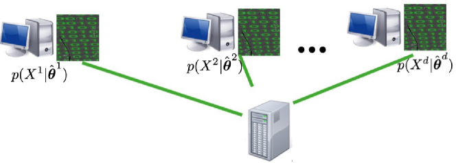
Figure 30: Illustration of the one-shot communication in distributed learning. Each local machine learns a probability model. The dataset is evenly partitioned $X=X^{1}\cup X^{2}\cup\cdots\cup X^{d}.$

Problem Setting

Suppose we have a dataset $X=\{\boldsymbol{x}_{j},~{}j=1,2,...,N\}$ of size $N$, i.i.d. drawn from a probabilistic model $p({\boldsymbol{x}}|\boldsymbol{\theta}^{*})$ within a parametric family $\mathcal{P}=\{p(\boldsymbol{x}|\boldsymbol{\theta}):\boldsymbol{\theta}\in\Theta\}$; here $\boldsymbol{\theta}^{*}$ is the unknown true parameter that we want to estimate based on $X$. In the distributed setting, the dataset $X$ is partitioned into $d$ disjoint subsets, $X=\bigcup_{k=1}^{d}X^{k}$, where $X^{k}$ denotes the $k$-th subset which we assume is stored in a local machine. For simplicity, we assume all the subsets have the same data size ($N/d$). The traditional maximum likelihood estimator (MLE) provides a natural way for estimating the true parameter $\boldsymbol{\theta}^{*}$ based on the whole dataset $X$,

$$\text{Global MLE:}\quad\boldsymbol{\hat{\theta}}_{\mathrm{mle}}=\operatorname*{arg\,max}_{\boldsymbol{\theta}\in\Theta}\sum_{k=1}^{d}\sum_{j=1}^{N/d}\log p({\boldsymbol{x}}^{k}_{j}\mid\boldsymbol{\theta}),\quad\text{where }X^{k}=\{{\boldsymbol{x}}^{k}_{j}\}.$$ (0.129)

However, directly calculating the global MLE is challenging due to the distributed partition of the dataset. Although distributed optimization algorithms exist (e.g., Boyd et al., 2011; Shamir et al., 2014), they require iterative communication between the local machines and a fusion center, which can be very time consuming in distributed settings, for which the number of communication rounds forms the main bottleneck (regardless of the amount of information communicated at each round).

We instead consider a simpler one-shot approach that first learns a set of local models based on each subset, and then send them to a fusion center in which they are combined into a global model that captures all the information. We assume each of the local models is estimated using a MLE based on subset $X^{k}$ from the $k$-th machine:

$$\text{Local MLE:}\quad\boldsymbol{\hat{\theta}}_{k}=\operatorname*{arg\,max}_{\boldsymbol{\theta}\in\Theta}\sum_{j=1}^{N/d}\log p(\boldsymbol{x}^{k}_{j}\mid\boldsymbol{\theta}),~{}~{}\text{where}~{}~{}k\in[d]=\{1,2,\cdots,d\}.$$ (0.130)

The major problem is how to combine these local models into a global model. The simplest way is to linearly average all local MLE parameters:

$$\text{Linear Average:}\quad\boldsymbol{\hat{\theta}}_{\mathrm{linear}}=\frac{1}{d}\sum_{k=1}^{d}\boldsymbol{\hat{\theta}}_{k}.$$

Comprehensive theoretical analysis has been done for $\boldsymbol{\hat{\theta}}_{\mathrm{linear}}$ (e.g., Zhang et al., 2012b; Rosenblatt & Nadler, 2014), which show that it has an asymptotic MSE of $\mathbb{E}||\boldsymbol{\hat{\theta}}_{\mathrm{linear}}-\boldsymbol{\theta}^{*}||^{2}=O(N^{-1})$. In fact, it is equivalent to the global MLE $\boldsymbol{\hat{\theta}}_{\mathrm{mle}}$ up to the first order $O(N^{-1})$, and several improvements have been developed to improve the second order term (e.g., Zhang et al., 2012b; Huang & Huo, 2015).

Unfortunately, the linear averaging method can easily break down in practice, or is even not applicable when the underlying model is complex. For example, it may work poorly when the likelihood has multiple modes, or when there exist non-identifiable parameters for which different parameter values correspond to a same model (also known as the label-switching problem); models of this kind include latent variable models and neural networks, and appear widely in machine learning. In addition, the linear averaging method is obviously not applicable when the local models have different numbers of parameters (e.g., Gaussian mixtures with unknown numbers of components), or when the parameters are simply not additive (such as parameters with discrete or categorical values). Further discussions on the practical limitations of the linear averaging method can be found in Liu & Ihler (2014).

All these problems of linear averaging can be well addressed by a KL-averaging method which averages the model (instead of the parameters) by finding a geometric center of the local models in terms of KL divergence (Merugu & Ghosh, 2003; Liu & Ihler, 2014). Specifically, it finds a model $p(\boldsymbol{x}|\boldsymbol{\theta}_{\mathrm{KL}}^{*})$ where $\boldsymbol{\theta}_{\mathrm{KL}}^{*}$ is obtained by

$$\boldsymbol{\theta}_{\mathrm{KL}}^{*}=\operatorname*{arg\,min}_{\boldsymbol{\theta}}\sum_{k=1}^{d}\mathrm{KL}(p(\boldsymbol{x}|\boldsymbol{\hat{\theta}}_{k})\mid\mid p(\boldsymbol{x}|\boldsymbol{\theta}))$$ (0.131)

The optimization of (0.131) is equivalent to,

$$\text{Exact KL Estimator: }\quad\boldsymbol{\theta}_{\mathrm{KL}}^{*}=\operatorname*{arg\,max}_{\boldsymbol{\theta}\in\Theta}\bigg{\{}\eta(\boldsymbol{\theta})\equiv\sum_{k=1}^{d}\int p(\boldsymbol{x}\mid\boldsymbol{\hat{\theta}}_{k})\log p(\boldsymbol{x}\mid\boldsymbol{\theta})d\boldsymbol{x}\bigg{\}}.$$ (0.132)

Liu & Ihler (2014) studied the theoretical properties of the KL-averaging method, and showed that it exactly recovers the global MLE, that is, $\boldsymbol{\theta}_{\mathrm{KL}}^{*}={\boldsymbol{\hat{\theta}}}_{\mathrm{mle}}$, when the distribution family is a full exponential family, and achieves an optimal asymptotic error rate (up to the second order) among all the possible combination methods of $\{\boldsymbol{\hat{\theta}}_{k}\}$. Despite the attractive properties, the exact KL-averaging is not computationally tractable except for very simple models. Liu & Ihler (2014) suggested a naive bootstrap method for approximation: it draws parametric bootstrap sample $\{\boldsymbol{\widetilde{x}}^{k}_{j}\}_{j=1}^{n}$ from each local model $p(\boldsymbol{x}|\boldsymbol{\hat{\theta}}_{k})$, $k\in[d]$ and use it to approximate each integral in (0.132). The optimization in (0.132) then reduces to a tractable one,

$$\text{KL-Naive Estimator:}\quad\boldsymbol{\hat{\theta}}_{\mathrm{KL}}=\operatorname*{arg\,max}_{\boldsymbol{\theta}\in\Theta}\bigg{\{}\hat{\eta}(\boldsymbol{\theta})\equiv\frac{1}{n}\sum_{k=1}^{d}\sum_{j=1}^{n}\log p(\boldsymbol{\widetilde{x}}^{k}_{j}\mid\boldsymbol{\theta})\bigg{\}}.$$ (0.133)

Intuitively, we can treat each $\widetilde{X}_{k}=\{\boldsymbol{\widetilde{x}}^{k}_{j}\}_{j=1}^{n}$ as an approximation of the original subset $X^{k}=\{\boldsymbol{{x}}^{k}_{j}\}_{j=1}^{N/d}$, and hence can be used to approximate the global MLE in (0.129).

Unfortunately, as the theoretical results shown in the next section, the accuracy of $\boldsymbol{\hat{\theta}}_{\mathrm{KL}}$ critically depends on the bootstrap sample size $n$, and one would need $n$ to be nearly as large as the original data size $N/d$ to make $\boldsymbol{\hat{\theta}}_{\mathrm{KL}}$ achieve the baseline asymptotic rate $O(N^{-1})$ that the simple linear averaging achieves; this is highly undesirably since $N$ is often assumed to be large in distributed learning settings.

Importance-Weighted Estimator to Bootstrapped Model Aggregation

In order to reduce the variance induced from the bootstrapped samples in  (0.133), we propose two variance reduction techniques for improving the KL-averaging estimates and discuss their theoretical and practical properties. We start with a concrete analysis on the $\mathrm{KL}$-naive estimator $\boldsymbol{\hat{\theta}}_{\mathrm{KL}},$ which was missing in Liu & Ihler (2014). Then we introduce a baseline control variates estimator method by leveraging the correlation of bootstrap samples $\{\boldsymbol{\widetilde{x}}^{k}_{j}\}_{j=1}^{n}$ among different local models $p(\boldsymbol{x}|\boldsymbol{\hat{\theta}}_{k}),$ $k=1,\cdots,d.$ While such method can only be used under the setting as that of the linear-averaging method, which limits its application. To overcome such a limitation, we finally propose a $\mathrm{KL}$-weighted estimator method, which overcomes all limitations of linear-averaging method.

The theoretical results provided in this chapter is based on the following assumptions of the probability model.

Assumption 18.

1. $\log p(\boldsymbol{x}\mid\boldsymbol{\theta}),$ $\frac{\partial\log p(\boldsymbol{x}\mid\boldsymbol{\theta})}{\partial\boldsymbol{\theta}},$ and $\frac{\partial^{2}\log p(\boldsymbol{x}\mid\boldsymbol{\theta})}{\partial\boldsymbol{\theta}\partial\boldsymbol{\theta}^{\top}}$ are continuous for $\forall~{}\boldsymbol{x}\in\mathcal{X}$ and $\forall~{}\boldsymbol{\theta}\in\Theta;$ 2. $\frac{\partial^{2}\log p(\boldsymbol{x}\mid\boldsymbol{\theta})}{\partial\boldsymbol{\theta}\partial\boldsymbol{\theta}^{\top}}$ is positive definite and $C_{1}\leq\|\frac{\partial^{2}\log p(\boldsymbol{x}\mid\boldsymbol{\theta})}{\partial\boldsymbol{\theta}\partial\boldsymbol{\theta}^{\top}}\|\leq C_{2}$ in a neighbor of $\boldsymbol{\theta}^{*}$ for $\forall~{}x\in\mathcal{X}$, and $C_{1}$, $C_{2}$ are some positive constants.

$\mathrm{KL}$-naive estimator to distributed model aggregation

In the following, we first prove ${\boldsymbol{\hat{\theta}}}_{\mathrm{KL}}$ provides a consistent estimation of the ground truth minimized model estimator $\boldsymbol{\theta}_{\mathrm{KL}}^{*}$ and the mean square error (MSE) between ${\boldsymbol{\hat{\theta}}}_{\mathrm{KL}}$ and $\boldsymbol{\theta}_{\mathrm{KL}}^{*}$ has an error rate $O(\frac{1}{dn}),$ where $d$ is the number of the local machines and $n$ is the number of the bootstrapped samples.

Theorem 19.

Under Assumption 32, ${\boldsymbol{\hat{\theta}}}_{\mathrm{KL}}$ is a consistent estimator of $\boldsymbol{\theta}_{\mathrm{KL}}^{*}$ as $n\to\infty$, and

$$\mathbb{E}({\boldsymbol{\hat{\theta}}}_{\mathrm{KL}}-\boldsymbol{\theta}_{\mathrm{KL}}^{*})=o(\frac{1}{dn}),\quad\mathbb{E}\|{\boldsymbol{\hat{\theta}}}_{\mathrm{KL}}-\boldsymbol{\theta}_{\mathrm{KL}}^{*}\|^{2}=O(\frac{1}{dn}),$$

where $d$ is the number of machines and $n$ is the bootstrap sample size for each local model $p(\boldsymbol{x}\mid\boldsymbol{\hat{\theta}}_{k})$.

The proof of Theorem 19 is provided in the Appendix Proofs of Theorems in Chapter. Based on the MSE between the exact $\mathrm{KL}$ estimator $\boldsymbol{\theta}_{\mathrm{KL}}^{*}$ and the true parameter $\boldsymbol{\theta}^{*}$ provided in Liu & Ihler (2014), it is easy to derive that the MSE between $\boldsymbol{\hat{\theta}}_{\mathrm{KL}}$ and the true parameter $\boldsymbol{\theta}^{*}$ satisfies

$$\mathbb{E}\|\boldsymbol{\hat{\theta}}_{\mathrm{KL}}-\boldsymbol{\theta}^{*}\|^{2}\approx\mathbb{E}\|\boldsymbol{\hat{\theta}}_{\mathrm{KL}}-\boldsymbol{\theta}^{*}_{\mathrm{KL}}\|^{2}+\mathbb{E}\|\boldsymbol{\theta}_{\mathrm{KL}}^{*}-\boldsymbol{\theta}^{*}\|^{2}=O(N^{-1}+(dn)^{-1}).$$ (0.134)

To guarantee the MSE rate between $\boldsymbol{\hat{\theta}}_{\mathrm{KL}}$ and $\boldsymbol{\theta}^{*}$ has the rate order $O(N^{-1})$, as what is achieved by the simple linear averaging, we need to draw $dn\gtrsim N$ bootstrap data points in total, which is undesirable since $N$ is often assumed to be very large by the assumption of distributed learning setting (one exception is when the data is distributed due to privacy constraint, in which case $N$ may be relatively small).

Therefore, it is a critical task to develop more accurate methods that can reduce the noise introduced by the bootstrap process. In the sequel, we introduce two variance reduction techniques to achieve this goal. One is based a (linear) control variates method that improves $\boldsymbol{\hat{\theta}}_{\mathrm{KL}}$ using a linear correction term, and another is a multiplicative control variates method that modifies the M-estimator in (0.133) by assigning each bootstrap data point with a positive weight to cancel the noise. We show that both method achieves a higher $O(N^{-1}+(dn^{2})^{-1})$ rate under mild assumptions, while the second method has more attractive practical advantages.

Proposed Baseline Control Variates Estimator

The control variates method is a technique for variance reduction on Monte Carlo estimation (e.g., Wilson, 1984). It introduces a set of correlated auxiliary random variables with known expectations or asymptotics (referred as the control variates), to balance the variation of the original estimator. In our case, since each bootstrapped subsample $\widetilde{X}^{k}=\{\boldsymbol{\widetilde{x}}^{k}_{j}\}_{j=1}^{n}$ is know to be drawn from the local model $p(\boldsymbol{x}\mid\boldsymbol{\hat{\theta}}_{k})$, we can construct a control variate by re-estimating the local model based on $\widetilde{X}^{k}$:

$$\text{Bootstrapped Local MLE:}\quad\boldsymbol{\widetilde{\theta}}_{k}=\operatorname*{arg\,max}_{\boldsymbol{\theta}\in\Theta}\sum_{j=1}^{n}\log p(\boldsymbol{\widetilde{x}}^{k}_{j}\mid\boldsymbol{\theta}),\quad\mathrm{for}~{}~{}k\in[d],$$ (0.135)

where $\boldsymbol{\widetilde{\theta}}_{k}$ is known to converge to $\boldsymbol{\hat{\theta}}_{k}$ asymptotically. This allows us to define the following control variates estimator:

$$\text{KL-Control Estimator:}\quad\boldsymbol{\hat{\theta}}_{\mathrm{KL}-C}=\boldsymbol{\hat{\theta}}_{\mathrm{KL}}+\sum_{k=1}^{d}\boldsymbol{\mathfrak{B}}_{k}(\boldsymbol{\widetilde{\theta}}_{k}-\boldsymbol{\hat{\theta}}_{k}),$$ (0.136)

where $\boldsymbol{\mathfrak{B}_{k}}$ is a matrix chosen to minimize the asymptotic variance of $\boldsymbol{\hat{\theta}}_{\mathrm{KL}-C}$; our derivation shows that the asymptotically optimal $\boldsymbol{\mathfrak{B}_{k}}$ has a form of

$$\boldsymbol{\mathfrak{B}}_{k}=-(\sum_{k=1}^{d}I(\boldsymbol{\hat{\theta}}_{k}))^{-1}I(\boldsymbol{\hat{\theta}}_{k}),\quad k\in[d],$$ (0.137)

where $I(\boldsymbol{\hat{\theta}}_{k})$ is the empirical Fisher information matrix of the local model $p(\boldsymbol{x}\mid\boldsymbol{\hat{\theta}}_{k})$. Note that this differentiates our method from the typical control variates methods where $\boldsymbol{\mathfrak{B}}_{k}$ is instead estimated using empirical covariance between the control variates and the original estimator (in our case, we can not directly estimate the covariance because $\boldsymbol{\hat{\theta}}_{\mathrm{KL}}$ and $\boldsymbol{\widetilde{\theta}}_{k}$ are not averages of i.i.d. samples).The procedure of our method is summarized in Algorithm 11. Note that the form of (0.136) shares some similarity with the one-step estimator in Huang & Huo (2015), but Huang & Huo (2015) focuses on improving the linear averaging estimator, and is different from our setting.

We analyze the asymptotic property of the estimator $\boldsymbol{\hat{\theta}}_{\mathrm{KL}-C}$, and summarize it as follows.

Theorem 20.

Under Assumption (32), $\boldsymbol{\hat{\theta}}_{\mathrm{KL}-C}$ is a consistent estimator of $\boldsymbol{\theta}_{\mathrm{KL}}^{*}$ as $n\to\infty,$ and its asymptotic MSE is guaranteed to be smaller than the KL-naive estimator ${\boldsymbol{\hat{\theta}}}_{\mathrm{KL}}$, that is,

$$n\mathbb{E}\|\boldsymbol{\hat{\theta}}_{\mathrm{KL}-C}-\boldsymbol{\theta}_{\mathrm{KL}}^{*}\|^{2}<n\mathbb{E}\|{\boldsymbol{\hat{\theta}}}_{\mathrm{KL}}-\boldsymbol{\theta}_{\mathrm{KL}}^{*}\|^{2},~{}~{}~{}~{}~{}~{}\text{as}~{}~{}n\to\infty.$$

In addition, when $N>n\times d$, the $\boldsymbol{\hat{\theta}}_{\mathrm{KL}-C}$ has “zero-variance” in that $\mathbb{E}\|{\boldsymbol{\hat{\theta}}}_{\mathrm{KL}}-\boldsymbol{\theta}_{\mathrm{KL}}^{*}\|^{2}=O((dn^{2})^{-1})$. Further, in terms of estimating the true parameter, we have

$$\mathbb{E}\|\boldsymbol{\hat{\theta}}_{\mathrm{KL}-C}-\boldsymbol{\theta}^{*}\|^{2}=O(N^{-1}+(dn^{2})^{-1}).$$ (0.138)

The proof is in the Appendix Proofs of Theorems in Chapter.

From (36), we can see that the MSE between $\boldsymbol{\hat{\theta}}_{\mathrm{KL}-C}$ and $\boldsymbol{\theta}^{*}$ reduces to $O(N^{-1})$ as long as $n\gtrsim(N/d)^{1/2}$, which is a significant improvement over the KL-naive method which requires $n\gtrsim N/d$. When the goal is to achieve an $O(\epsilon)$ MSE, we would just need to take $n\gtrsim 1/(d\epsilon)^{1/2}$ when $N>1/\epsilon$, that is, $n$ does not need to increase with $N$ when $N$ is very large.

Meanwhile, because $\boldsymbol{\hat{\theta}}_{\mathrm{KL}-C}$ requires a linear combination of $\boldsymbol{\hat{\theta}}_{k}$, $\boldsymbol{\widetilde{\theta}}_{k}$ and $\boldsymbol{\hat{\theta}}_{\mathrm{KL}}$, it carries the practical drawbacks of the linear averaging estimator as we discuss in Section Problem Setting. This motivates us to develop another KL-weighted method shown in the next section, which achieves the same asymptotical efficiency as $\boldsymbol{\hat{\theta}}_{\mathrm{KL}-C}$, while still inherits all the practical advantages of KL-averaging.

Algorithm 11 KL-Control Variates Method for Combining Local Models

1:  Input: Local model parameters $\{\boldsymbol{\hat{\theta}}_{k}\}_{k=1}^{d}$.

2:  Generate bootstrap data $\{\boldsymbol{\widetilde{x}}^{k}_{j}\}_{j=1}^{n}$ from each $p(\boldsymbol{x}|\boldsymbol{\hat{\theta}}_{k})$, for $k\in[d]$.

3:  Calculate the KL-Naive estimator, $\boldsymbol{\hat{\theta}}_{\mathrm{KL}}=\operatorname*{arg\,max}_{\boldsymbol{\theta}\in\Theta}\sum_{k=1}^{d}\frac{1}{n}\sum_{j=1}^{n}\log p(\boldsymbol{\widetilde{x}}^{k}_{j}|\boldsymbol{\theta}).$

4:  Re-estimate the local parameters $\widetilde{\boldsymbol{\theta}}_{k}$ via (0.135) based on the bootstrapped data subset $\{\boldsymbol{\widetilde{x}}^{k}_{j}\}_{j=1}^{n}$,   for $k\in[d]$.

5:  Estimate the empirical Fisher information matrix $I(\boldsymbol{\hat{\theta}}_{k})=\frac{1}{n}\sum_{j=1}^{n}\frac{\partial{\log p(\boldsymbol{\widetilde{x}}_{j}^{k}|\boldsymbol{\hat{\theta}}_{k})}}{\partial{\boldsymbol{\theta}}}{\frac{\partial{\log p(\boldsymbol{\widetilde{x}}_{j}^{k}|\boldsymbol{\hat{\theta}}_{k})}}{\partial{\boldsymbol{\theta}}}}^{\top}$, for $k\in[d]$.

6:  Ouput: The parameter $\boldsymbol{\hat{\theta}}_{\mathrm{KL}-C}$ of the combined model is given by (0.136) and (0.137).

KL-Weighted Estimator

Our KL-weighted estimator is based on directly modifying the M-estimator for $\boldsymbol{\hat{\theta}}_{\mathrm{KL}}$ in (0.133), by assigning each bootstrap data point $\boldsymbol{\widetilde{x}}_{j}^{k}$ a positive weight according to the probability ratio $p(\boldsymbol{\widetilde{x}}_{j}^{k}\mid\boldsymbol{\hat{\theta}}_{k})/p(\boldsymbol{\widetilde{x}}_{j}^{k}\mid\boldsymbol{\widetilde{\theta}}_{k})$ of the actual local model $p(x|\boldsymbol{\hat{\theta}}_{k})$ and the re-estimated model $p(x|\boldsymbol{\widetilde{\theta}}_{k})$ in (0.135). Here the probability ratio acts like a multiplicative control variate (Nelson, 1987), which has the advantage of being positive and applicable to non-identifiable, non-additive parameters. Our KL-weighted estimator is defined as

$${\boldsymbol{\hat{\theta}}}_{\mathrm{KL}-W}=\operatorname*{arg\,max}_{\boldsymbol{\theta}\in\Theta}\bigg{\{}\widetilde{\eta}(\boldsymbol{\theta})\equiv\sum_{k=1}^{d}\frac{1}{n}\sum_{j=1}^{n}\frac{p(\boldsymbol{\widetilde{x}}_{j}^{k}|\boldsymbol{\hat{\theta}}_{k})}{p(\boldsymbol{\widetilde{x}}_{j}^{k}|\boldsymbol{\widetilde{\theta}}_{k})}\log p(\boldsymbol{\widetilde{x}}_{j}^{k}|\boldsymbol{\theta})\bigg{\}}.$$ (0.139)

We first show that this weighted estimator $\widetilde{\eta}(\boldsymbol{\theta})$ gives a more accurate estimation of $\eta(\boldsymbol{\theta})$ in (0.132) than the straightforward estimator $\hat{\eta}(\boldsymbol{\theta})$ defined in (0.133) for any $\boldsymbol{\theta}\in\Theta$.

Lemma 21.

As $n\to\infty$, $\widetilde{\eta}(\boldsymbol{\theta})$ is a more accurate estimator of $\eta(\boldsymbol{\theta})$ than $\hat{\eta}(\boldsymbol{\theta})$, in that

$$n\mathrm{Var}(\widetilde{\eta}(\boldsymbol{\theta}))\leq n\mathrm{Var}(\hat{\eta}(\boldsymbol{\theta})),~{}~{}~{}~{}~{}\text{as }n\to\infty,~{}~{}\quad\text{for any }\boldsymbol{\theta}\in\Theta.$$ (0.140)

This estimator is motivated by Henmi et al. (2007) in which the same idea is applied to reduce the asymptotic variance in importance sampling. Similar result is also found in Hirano et al. (2003), in which it is shown that a similar weighted estimator with estimated propensity score is more efficient than the estimator using true propensity score in estimating the average treatment effects. Although being a very powerful tool, results of this type seem to be not widely known in machine learning, except several applications in semi-supervised learning (Sokolovska et al., 2008; Kawakita & Kanamori, 2013), and off-policy learning (Li et al., 2015).

We go a step further to analyze the asymptotic property of our weighted M-estimator $\boldsymbol{\hat{\theta}}_{\mathrm{KL}-W}$ that maximizes $\widetilde{\eta}(\boldsymbol{\theta})$. It is natural to expect that the asymptotic variance of $\boldsymbol{\hat{\theta}}_{\mathrm{KL}-W}$ is smaller than that of $\boldsymbol{\hat{\theta}}_{\mathrm{KL}}$ based on maximizing $\hat{\eta}(\boldsymbol{\theta})$; this is shown in the following theorem.

Theorem 22.

Under Assumption 32, $\boldsymbol{\hat{\theta}}_{\mathrm{KL}-W}$ is a consistent estimator of $\boldsymbol{\theta}_{\mathrm{KL}}^{*}$ as $n\to\infty,$ and has a better asymptotic variance than $\boldsymbol{\hat{\theta}}_{\mathrm{KL}}$, that is,

$$n\mathbb{E}\|\boldsymbol{\hat{\theta}}_{\mathrm{KL}-W}-\boldsymbol{\theta}_{\mathrm{KL}}^{*}\|^{2}\leq n\mathbb{E}\|\boldsymbol{\hat{\theta}}_{\mathrm{KL}}-\boldsymbol{\theta}_{\mathrm{KL}}^{*}\|^{2},~{}~{}~{}~{}~{}\text{when $n\to\infty$}.$$

When $N>n\times d$, we have $\mathbb{E}\|\boldsymbol{\hat{\theta}}_{\mathrm{KL}-W}-\boldsymbol{\theta}_{\mathrm{KL}}^{*}\|^{2}=O(({dn^{2}})^{-1})$ as $n\to\infty.$ Further, its MSE for estimating the true parameter $\boldsymbol{\theta}^{*}$ is

$$\mathbb{E}\|\boldsymbol{\hat{\theta}}_{\mathrm{KL}-W}-\boldsymbol{\theta}^{*}\|^{2}=O(N^{-1}+(dn^{2})^{-1}).$$ (0.141)

The proof is in Appendix C. This result is parallel to Theorem 20 for the linear control variates estimator $\boldsymbol{\hat{\theta}}_{\mathrm{KL}-C}$. Similarly, it reduces to an $O(N^{-1})$ rate once we take $n\gtrsim(N/d)^{1/2}$.

Meanwhile, unlike the linear control variates estimator, $\boldsymbol{\hat{\theta}}_{\mathrm{KL}-W}$ inherits all the practical advantages of KL-averaging: it can be applied whenever the KL-naive estimator can be applied, including for models with non-identifiable parameters, or with different numbers of parameters. The implementation of $\boldsymbol{\hat{\theta}}_{\mathrm{KL}-W}$ is also much more convenient (see Algorithm 12), since it does not need to calculate the Fisher information matrix as required by Algorithm 11.

Algorithm 12 KL-Weighted Method for Combining Local Models

1:  Input: Local MLEs $\{\boldsymbol{\hat{\theta}}_{k}\}_{k=1}^{d}$.

2:  Generate bootstrap sample $\{\boldsymbol{\widetilde{x}}^{k}_{j}\}_{j=1}^{n}$ from each $p(\boldsymbol{x}|\boldsymbol{\hat{\theta}}_{k})$, for $k\in[d].$

3:  Re-estimate the local model parameter $\boldsymbol{\widetilde{\theta}}_{k}$ in (0.135) based on bootstrap subsample $\{\boldsymbol{\widetilde{x}}^{k}_{j}\}_{j=1}^{n}$, for each $k\in[d].$

4:  Output: The parameter $\boldsymbol{\hat{\theta}}_{\mathrm{KL}-W}$ of the combined model is given by (0.139).

Empirical Experiments

We study the empirical performance of our proposed two methods on both simulated and real world datasets. We first numerically verify the convergence rates predicted by our theoretical results using simulated data, and then demonstrate the effectiveness of our methods in a challenging setting when the number of parameters of the local models are different as decided by Bayesian information criterion (BIC). Finally, we conclude our experiments by testing our methods on a set of real world datasets.

The models we tested include probabilistic principal components analysis (PPCA), mixture of PPCA and Gaussian Mixtures Models (GMM). PPCA model is defined with the help of a hidden variable $\boldsymbol{t}$,

$$p(\boldsymbol{x}~{}|~{}\boldsymbol{\theta})=\int p(\boldsymbol{x}~{}|~{}\boldsymbol{t};~{}\boldsymbol{\theta})p(\boldsymbol{t}~{}|~{}\boldsymbol{\theta})d\boldsymbol{t},$$

where $p(\boldsymbol{x}\mid\boldsymbol{t};~{}\boldsymbol{\theta})=\mathcal{N}(\boldsymbol{x};~{}\boldsymbol{\mu}+W\boldsymbol{t},\sigma^{2}),$ and the distribution of hidden variable $\boldsymbol{t}$ is $p(\boldsymbol{t}\mid\boldsymbol{\theta})=\mathcal{N}(\boldsymbol{t};~{}\boldsymbol{0},\boldsymbol{I})$ and $\boldsymbol{\theta}=\{\boldsymbol{\mu},~{}W,~{}\sigma^{2}\}$. The mixture of PPCA is $p(\boldsymbol{x}\mid\boldsymbol{\theta})=\sum_{s=1}^{m}\alpha_{s}p_{s}(\boldsymbol{x}\mid\boldsymbol{\theta}_{s})$, where $\boldsymbol{\theta}=\{\alpha_{s},\boldsymbol{\theta}_{s}\}_{s=1}^{m}$ and each $p_{s}(\boldsymbol{x}\mid\boldsymbol{\theta}_{s})$ is a PPCA model.

GMM is given by $p(\boldsymbol{x}\mid\boldsymbol{\theta})=\sum_{s=1}^{m}\alpha_{s}\mathcal{N}(\boldsymbol{\mu}_{s},\Sigma_{s})$ where $\mathcal{N}(\boldsymbol{\mu}_{s},\Sigma_{s})$ is a multivariate Gaussian distribution and the parameters are $\boldsymbol{\theta}=(\alpha_{s},\boldsymbol{\mu}_{s},\Sigma_{s}).$

Because all these models are latent variable models with unidentifiable parameters, the direct linear averaging method is not applicable. For GMM, it is still possible to use a matched linear averaging which matches the mixture components of the different local models by minimizing a symmetric $\mathrm{KL}$ divergence; the same idea can be used on our linear control variates method to make it applicable to GMM. On the other hand, because the parameters of PPCA-based models are unidentifiable up to arbitrary orthonormal transforms, linear averaging and linear control variates can no longer be applied easily. We use expectation maximization (EM) to learn the parameters in all these three models.

Numerical Verification of the Convergence Rates

We start with verifying the convergence rates in (0.134), (36) and (39) of MSE $\mathbb{E}||\boldsymbol{\hat{\theta}}-\boldsymbol{\theta}^{*}||^{2}$ of the different estimators for estimating the true parameters. Because there is also an non-identifiability problem in calculating the MSE, we again use the symmetric KL divergence to match the mixture components, and evaluate the MSE on $WW^{\top}$ to avoid the non-identifiability w.r.t. orthonormal transforms.

To verify the convergence rates w.r.t. $n$, we fix $d$ and let the total dataset $N$ be very large so that $N^{-1}$ is negligible. The dimensions of the PPCA models in (a)-(b) are 5, and that of GMM in (c) is 3. The numbers of mixture components in (b)-(c) are 3. Linear averaging and KL-Control are not applicable for the PPCA-based models, and are not shown in (a) and (b). Figure 31 shows the results when we vary $n$, where we can see that the MSE of KL-naive ${\boldsymbol{\hat{\theta}}}_{\mathrm{KL}}$ is $O(n^{-1})$ while that of KL-control $\hat{\boldsymbol{\theta}}_{\mathrm{KL}-C}$ and KL-weighted $\hat{\boldsymbol{\theta}}_{\mathrm{KL}-W}$ are $O(n^{-2})$; both are consistent with our results in (0.134), (36) and (39).

In Figure 32(a), we increase the number $d$ of local machines, while using a fix $n$ and a very large $N$, and find that both $\boldsymbol{\hat{\theta}}_{\mathrm{KL}}$ and $\boldsymbol{\hat{\theta}}_{\mathrm{KL}-W}$ scales as $O(d^{-1})$ as expected. Note that since the total observation data size $N$ is fixed, the number of data in each local machine is $(N/d)$ and it decreases as we increase $d$. It is interesting to see that the performance of the KL-based methods actually increases with more partitions; this is, of course, with a cost of increasing the total bootstrap sample size $dn$ as $d$ increases. Figure 32(b) considers a different setting, in which we increase $d$ when fixing the total observation data size $N$, and the total bootstrap sample size $n_{\mathrm{tot}}=n\times d$. According to (0.134) and (39), the MSEs of $\boldsymbol{\hat{\theta}}_{\mathrm{KL}}$ and $\boldsymbol{\hat{\theta}}_{\mathrm{KL}-W}$ should be about $O(n_{\mathrm{tot}}^{-1})$ and $O(dn_{\mathrm{tot}}^{-2})$ respectively when $N$ is very large, and this is consistent with the results in Figure 32(b). It is interesting to note that the MSE of $\boldsymbol{\hat{\theta}}_{\mathrm{KL}}$ is independent with $d$ while that of $\boldsymbol{\hat{\theta}}_{\mathrm{KL}-W}$ increases linearly with $d$. This is not conflict with the fact that $\boldsymbol{\hat{\theta}}_{\mathrm{KL}-W}$ is better than $\boldsymbol{\hat{\theta}}_{\mathrm{KL}}$, since we always have $d\leq n_{\mathrm{tot}}$.

Figure 32(c) shows the result when we set $n=(N/d)^{\alpha}$ and vary $\alpha$, where we find that $\boldsymbol{\hat{\theta}}_{\mathrm{KL}-W}$ quickly converges to the global MLE as $\alpha$ increases, while the KL-naive estimator $\boldsymbol{\hat{\theta}}_{\mathrm{KL}}$ converges significantly slower. Figure 32(d) demonstrates the case when we increase $N$ while fix $d$ and $n$, where we see our KL-weighted estimator $\boldsymbol{\hat{\theta}}_{\mathrm{KL}-W}$ matches closely with $N$, except when $N$ is very large in which case the $O((dn^{2})^{-1})$ term starts to dominate, while KL-naive is much worse. We also find the linear averaging estimator performs poorly, and does not scale with $O(N^{-1})$ as the theoretical rate claims; this is due to unidentifiable orthonormal transform in the PPCA model that we test on.

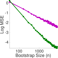
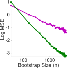
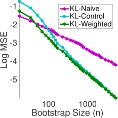
(a) PPCA	(b) Mixture of PPCA	(c) GMM

Figure 31: Results on different models with simulated data when we change the bootstrap sample size $n$, with fixed $d=10$ and $N=6\times 10^{7}$.

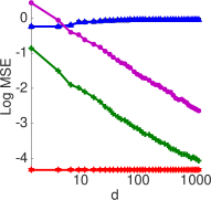
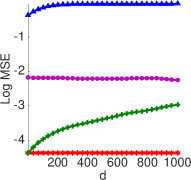
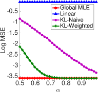
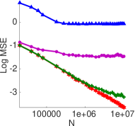
(a) Fix $N$ and $n$	(b) Fix $N$ and $n_{\mathrm{tot}}$	(c) Fix $N$, $n=(\frac{N}{d})^{\alpha}$ and $d$	(d) Fix $n$ and $d$

Figure 32: Further experiments on PPCA with simulated data. (a) varying $n$ with fixed $N=5\times 10^{7}$. (b) varying $d$ with $N=5\times 10^{7}$, $n_{\mathrm{tot}}=n\times d=3\times 10^{5}$. (c) varying $\alpha$ with $n=(\frac{N}{d})^{\alpha}$, $N=10^{7}$ and $d$. (d) varying $N$ with $n=10^{3}$ and $d=20$. The dimension of data $\boldsymbol{x}$ is 5 and the dimension of latent variables $\boldsymbol{t}$ is 4.

Gaussian Mixture with Unknown Number of Components

We further apply our methods to a more challenging setting for distributed learning of GMM when the number of mixture components is unknown. In this case, we first learn each local model with EM and decide its number of components using BIC selection. Both linear averaging and KL-control $\boldsymbol{\hat{\theta}}_{\mathrm{KL}-C}$ are not applicable in this setting, and and we only test KL-naive $\boldsymbol{\hat{\theta}}_{\mathrm{KL}}$ and KL-weighted $\boldsymbol{\hat{\theta}}_{\mathrm{KL}-W}$. Since the MSE is also not computable due to the different dimensions, we evaluate $\boldsymbol{\hat{\theta}}_{\mathrm{KL}}$ and $\boldsymbol{\hat{\theta}}_{\mathrm{KL}-W}$ using the log-likelihood on a hold-out testing dataset as shown in Figure 33. We can see that $\boldsymbol{\hat{\theta}}_{\mathrm{KL}-W}$ generally outperforms $\boldsymbol{\hat{\theta}}_{\mathrm{KL}}$ as we expect, and the relative improvement increases significantly as the dimension of the observation data $\boldsymbol{x}$ increases. This suggests that our variance reduction technique works very efficiently in high dimension problems.

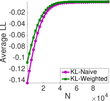
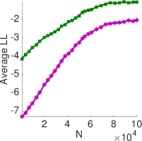
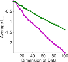
(a) Dimension of $\boldsymbol{x}$ = 3	(b) Dimension of $\boldsymbol{x}$ = 80	(c) varying the dimension of $\boldsymbol{x}$

Figure 33: GMM with the number of mixture components estimated by Bayesian information criterion. We set $n=600$ and the true number of mixtures to be 10 in all the cases. (a)-(b) vary the total data size $N$ when the dimension of $\boldsymbol{x}$ is 3 and 80, respectively. (c) varies the dimension of the data with fixed $N=10^{5}$. The y-axis is the testing $\log$ likelihood compared with that of global MLE.

Results on Real World Datasets

Finally, we apply our methods to several real world datasets, including the SensIT Vehicle dataset on which mixture of PPCA is tested, and the Covertype and Epsilon datasets on which GMM is tested. From Figure 34, we can see that our KL-Weight and KL-Control (when it is applicable) again perform the best. The (matched) linear averaging performs poorly on GMM (Figure 34(b)-(c)), while is not applicable on mixture of PPCA.

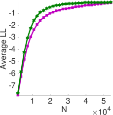
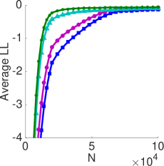
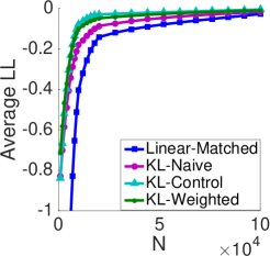
(a) Mixture of PPCA, SensIT Vehicle	(b) GMM, Covertype	(c) GMM, Epsilon

Figure 34: Testing $\log$ likelihood (compared with that of global MLE) on real world datasets. (a) Learning Mixture of PPCA on SensIT Vehicle. (b)-(c) Learning GMM on Covertype and Epsilon. The number of local machines is 10 in all the cases, and the number of mixture components are taken to be the number of labels in the datasets. The dimension of latent variables in (a) is 90. For Epsilon dataset, the PCA is first applied and the top 100 principal components are chosen. Linear-matched and $\mathrm{KL}$-Control are not applicable on Mixture of PPCA and are not shown on (a).

Summary

This chapter addresses the model aggregation problem in distributed, or privacy-preserving learning. We consider the one-shot communication by sending the probabilistic models estimated from different local repositories $\{p(\boldsymbol{x}|\boldsymbol{\hat{\theta}}_{k})\}_{k=1}^{d}$ to a fusion center. The simple way is to linearly average the parameters of the local models, $\boldsymbol{\hat{\theta}}=\frac{1}{d}\sum_{j=1}^{d}\boldsymbol{\hat{\theta}}_{j}$. Although nearly asymptotically optimal error rates can be achieved, this linear-averaging method tends to degenerate in practical scenarios for models with non-convex log-likelihood or non-identifiable parameters (such as latent variable models and neural models), and is not applicable at all for models with non-additive parameters (e.g., when the parameters have discrete or categorical values, the number of parameters in local models are different, or the parameter dimensions of the local models are different). To overcome the limitations of the parameter-averaging based method, we instead find a joint model $p(\boldsymbol{x}|\boldsymbol{\hat{\theta}})$ which has a minimal sum of the $\mathrm{KL}$ divergence between each local model and the joint model, i.e., $\boldsymbol{\hat{\theta}}=\operatorname*{arg\,max}_{{\boldsymbol{\theta}}}\sum_{j=1}^{d}\mathrm{KL}(p(\boldsymbol{x}\mid\boldsymbol{\hat{\theta}}_{k})||p({\boldsymbol{x}}|{\boldsymbol{\theta}})).$ The similar objective has been used in optimizing the approximate distribution $q_{{\boldsymbol{\theta}}}({\boldsymbol{x}})$ in variational inference, $\min_{{\boldsymbol{\theta}}}\mathrm{KL}(q_{{\boldsymbol{\theta}}}({\boldsymbol{x}})||p({\boldsymbol{x}})).$ As the closed form of the integration induced from the $\mathrm{KL}$ divergence is unavailable in most cases (for most choices of $p(\boldsymbol{x}\mid\boldsymbol{\hat{\theta}}_{k})$, the integration cannot be analytically evaluated), we need to sample bootstrap data $\{\boldsymbol{\widetilde{x}}_{j}^{k}\}_{j=1}^{n}$ from each local model $p(\boldsymbol{x}\mid\boldsymbol{\hat{\theta}}_{k})$ to do naive Monte Carlo estimation of the integration. Unfortunately, this bootstrapped procedure induces large variance (the mean square error rate between the naive estimator and the ground truth value is $O(N^{-1}+(dn)^{-1})$), when $n$ is typically assumed to be small, which limits its application. In this chapter, we propose two effective variance reduction techniques to learn a joint model $p(\boldsymbol{x}|\boldsymbol{\hat{\theta}}),$ including a KL-weighted estimator that is both statistically efficient and widely applicable for even challenging practical scenarios. Theoretical analysis is provided to understand the statistical property of our proposed methods. The two estimators proposed in this chapter are unbiased and has MSE rate $O(N^{-1}+(d^{-1}n^{-2}),$ where $N$ is the size of the original dataset and $n$ is the size of the bootstrapped sample for each local model $p(\boldsymbol{x}\mid\boldsymbol{\hat{\theta}}_{k})$. We perform experiments on three different models, PPCA, mixture PPCA and GMM. A sufficient empirical experiments for the PPCA and GMM models on simulated datasets exactly verify the theoretical correctness of our proposed two estimators under different choices of $N$, $n$ and $d$. The empirical results on various real datasets demonstrate the practical power of our proposed $\mathrm{KL}$-averaging method when applied to latent variable model and multi-modal models with non-convex nature. Future directions include extending our methods to discriminant learning tasks, as well as the more challenging deep generative networks on which the exact MLE is not computationally tractable, and surrogate likelihood methods with stochastic gradient descent are needed. We note that the same KL-averaging problem also appears in the “knowledge distillation” problem in Bayesian deep neural networks (Korattikara et al., 2015), and it seems that our technique can be applied straightforwardly. Our $\mathrm{KL}$ averaging method can also be directly applied to optimize the approximate distribution in variational inference.

Conclusions and Future Works

In this thesis, we propose several approximate inference algorithms, which can be effectively applied to continuous-valued distributions and discrete-valued distributions. Traditional MCMC-based methods, which usually runs very long Markov chains to approximate the target distributions, have theoretical guarantee of the convergence of the chain to the target distribution but are very slow. Variational inference methods approximate the target distribution $p({\boldsymbol{x}})$ with an approximate distribution $q_{\phi}({\boldsymbol{x}})$ and optimize $\phi$, which are much faster but the predefined parametric distribution $q_{\phi}({\boldsymbol{x}})$ tends to give a poor approximation as $p({\boldsymbol{x}})$ might not be from the predefined parametric family. SVGD (Liu & Wang, 2016) is an alternative framework that integrates both the advantages of particle-based methods and variational algorithms. In this thesis, we propose several new methods in the framework of SVGD, where the original SVGD cannot be readily applied. The whole thesis can be summarized into three main pipelines. Our recently proposed approximate inference framework provide a powerful tool and new direction to perform faster and more accurate inference. While several new questions deserve to be investigated, which might ultimately improve current performance and further achieve the state-of-the-art results in approximate inference. We will discuss them in detail in each pipeline.

Approximate Inference on Continuous-valued Distribution

In the following, we first emphasize our contributions of approximate inference algorithms on continuous-valued distributions. Specifically, we propose a nonparametric adaptive importance sampling algorithm by decoupling the iteratively updated particles of SVGD $\{{\boldsymbol{x}}_{i}^{\ell}\}_{i=1}^{n}$ into two sets: leader particles ${\boldsymbol{x}}_{A}^{\ell}=\{{\boldsymbol{x}}_{i}^{\ell}\colon i\in A\}$ and follower particles ${\boldsymbol{x}}_{B}^{\ell}=\{{\boldsymbol{x}}_{i}^{\ell}\colon i\in B\}$, with $B=\{1,\ldots,n\}\setminus A$. The leader particles is applied to construct the transform and the follower particles are updated by the constructed transform, $\boldsymbol{x}_{i}^{\ell+1}\leftarrow\boldsymbol{x}_{i}^{\ell}+\epsilon{\boldsymbol{\phi}}_{\ell+1}(\boldsymbol{x}_{i}^{\ell}),~{}\forall i\in A\cup B,$ where ${\boldsymbol{\phi}}_{\ell+1}(\cdot)$ is constructed by only using particles in set $A,$

$$\!\!\!\!\!\!\!\!{\boldsymbol{\phi}}_{\ell+1}(\cdot)=\frac{1}{|A|}\sum_{j\in A}[\nabla\log p(\boldsymbol{x}_{j}^{\ell})k(\boldsymbol{x}_{j}^{\ell},\cdot)+\nabla_{\boldsymbol{x}_{j}^{\ell}}k(\boldsymbol{x}_{j}^{\ell},\cdot)].$$

With such a transform, the distribution of the updated particles $\{\boldsymbol{x}_{j}^{\ell}\}$ in ${\boldsymbol{x}}_{B}$ satisfies

$$q_{\ell}=({\boldsymbol{T}}_{\ell}\circ\cdots\circ{\boldsymbol{T}}_{1})\sharp q_{0},\quad\ell=1,\ldots,K,$$ (0.142)

where the importance proposal $q_{\ell}$ forms increasingly better approximation of the target $p$ as $\ell$ increases. Conditional on ${\boldsymbol{x}}_{A}^{\ell},$ particles in ${\boldsymbol{x}}_{B}^{\ell}$ are i.i.d. and hence can provide an unbiased estimation of the integral $\mathbb{E}_{{\boldsymbol{x}}\sim q_{\ell}}[\frac{p({\boldsymbol{x}})}{q_{\ell}({\boldsymbol{x}})}h({\boldsymbol{x}})]$ for any function $h({\boldsymbol{x}}).$ Our importance proposal is not restricted to the predefined distributional family as traditional adaptive importance sampling methods do. The $\mathrm{KL}$ divergence between the updated proposal $q_{\ell}$ and the target distribution is also maximally decreased in a functional space, which inherits from the theory of SVGD (Liu, 2017). We apply our proposed algorithm to evaluate the normalization constant of various probability models including restricted Boltzmann machine and deep generative model to demonstrate the effectiveness of our proposed algorithm, where the original SVGD cannot be applied in such tasks. We propose a novel sampling algorithm for continuous-valued target distribution when the gradient information of the target distribution is unavailable. iteratively updated by ${\boldsymbol{x}}_{i}\leftarrow{\boldsymbol{x}}_{i}+\frac{\epsilon}{n}\Delta{\boldsymbol{x}}_{i}$, where

$$\Delta{\boldsymbol{x}}_{i}\propto\sum_{j=1}^{n}\!w({\boldsymbol{x}}_{j})\big{[}\nabla\log\rho({\boldsymbol{x}}_{j})k({\boldsymbol{x}}_{j},{\boldsymbol{x}}_{i})+\nabla_{{\boldsymbol{x}}_{j}}k({\boldsymbol{x}}_{j},{\boldsymbol{x}}_{i})\big{]},$$ (0.143)

which replaces the true gradient $\nabla\log p({\boldsymbol{x}})$ with a surrogate gradient $\nabla\log\rho({\boldsymbol{x}})$ of an arbitrary auxiliary distribution $\rho({\boldsymbol{x}})$, and then uses an importance weight $w({\boldsymbol{x}}_{j}):=\rho({\boldsymbol{x}}_{j})/p({\boldsymbol{x}}_{j})$ to correct the bias introduced by the surrogate $\rho({\boldsymbol{x}})$. Perhaps surprisingly, we show that the new update can be derived as a standard SVGD update by using an importance weighted kernel $w({\boldsymbol{x}})k({\boldsymbol{x}},{\boldsymbol{x}}^{\prime})w({\boldsymbol{x}}^{\prime})$, and hence immediately inherits the theoretical proprieties of SVGD; for example, particles updated by (0.143) can be viewed as a gradient flow of KL divergence similar to the original SVGD (Liu, 2017). Empirical experiments demonstrate that our proposed gradient-free SVGD significantly outperforms gradient-free Markov Chain Monte Carlo sampling baselines on various probability models with intractable normalization constant and unavailable gradient information of the target distribution.

Approximate Inference on Discrte-valued Distribution

In the second part of the thesis, we propose two approximate inference algorithms on discrete-valued distributions. We propose a new algorithm to sample from the discrete-valued distributions. Our proposed algorithm is based on the fact that the discrete-valued distributions can be bijectively mapped to the piecewise continuous-valued distributions. Since the piecewise continuous-valued distributions are non-differentiable, gradient-based sampling algorithms cannot be applied in this setting. Our proposed sample-efficient GF-SVGD is a natural choice. To construct effective surrogate distributions $\rho({\boldsymbol{x}})$ in GF-SVGD, we propose a simple transformation, the inverse of dimension-wise Gaussian c.d.f., to transform the piecewise continuous-valued distributions to a simple form of continuous distributions. With such a straightforward transform, the effective surrogate distribution $\rho({\boldsymbol{x}})$ in GF-SVGD is natural to construct. Empirical experiments on large-scale discrete graphical models demonstrate the effectiveness of our proposed algorithm.

Principled Ensemble Method to Learn Binarized Neural Networks

As a direct application from sampling on discrete distributions, we propose a principled ensemble method to train the binarized neural networks (BNN). We train an ensemble of $n$ neural networks (NN) with the same architecture ($n\geq 2$). Let $\boldsymbol{W}_{i}^{b}$ be the binary weight of model $i$, for $i=1,\cdots,n$, and $p_{*}(\boldsymbol{W}_{i}^{b};D)$ be the target probability model with softmax layer as last layer given the data $D$. Learning the target probability model is framed as drawing $n$ samples $\{\boldsymbol{W}_{i}^{b}\}_{i=1}^{n}$ to approximate the posterior distribution $p_{*}(\boldsymbol{W}^{b};D)$. Let $p_{0}(w)$ be the base function, which is the product of the p.d.f. of the standard Gaussian distribution over the dimension $d.$ The distribution of $\boldsymbol{W}$ has the form $p_{c}(\boldsymbol{W};D)\propto p_{*}(\mathrm{sign}(\boldsymbol{W});D)p_{0}(\boldsymbol{W})$ with weight $\boldsymbol{W}$ and the $\mathrm{sign}$ function is applied to each dimension of $\boldsymbol{W}$. The surrogate probability model $\rho(\boldsymbol{W};D)$ is easily constructed by $\widetilde{p}(\sigma(\boldsymbol{W});D)p_{0}(\boldsymbol{W})$. Here $\widetilde{p}(\sigma(\boldsymbol{W});D)$ is a differentiable approximation of $p_{*}(\mathrm{sign}(\boldsymbol{W});D).$ Then an ensemble of models $\{\boldsymbol{W}_{i}\}_{i=1}^{n}$ is updated by GF-SVGD as follows, $\boldsymbol{W}_{i}\leftarrow\boldsymbol{W}_{i}+\frac{\epsilon_{i}}{\Omega}\Delta\boldsymbol{W}_{i}$, $\forall i=1,\cdots,n,$

$$\Delta\boldsymbol{W}_{i}\!\!\leftarrow\!\!\!\sum_{j=1}^{n}\!\gamma_{j}[\nabla_{\boldsymbol{W}}\log\rho(\boldsymbol{W}_{j};\!D_{i})k(\boldsymbol{W}_{j}\!,\!\boldsymbol{W}_{i})+\!\nabla_{\boldsymbol{W}_{j}}k(\boldsymbol{W}_{j}\!,\!\boldsymbol{W}_{i})]$$ (0.144)

where $D_{i}$ is batch data $i$ and $\mu_{j}=\rho(\boldsymbol{W}_{j};D_{i})/p_{c}(\boldsymbol{W}_{j};D_{i})$, $H(t)\overset{\mathrm{def}}{=}\sum_{j=1}^{n}\mathbb{I}(\mu_{j}\geq t)/n$, $\gamma_{j}=(H(\boldsymbol{W}_{j}))^{-1}$ and $\Omega=\sum_{j=1}^{n}\gamma_{j}$.

We compare our ensemble algorithm with typical ensemble method using bagging and AdaBoost (BENN, Zhu et al. (2018)), BNN (Hubara et al., 2016) and BNN+(Darabi et al., 2018). Both BNN and BNN+ are trained on a single model with same network structure. Our proposed ensemble algorithm achieves the highest accuracy among all three ensemble by using AlexNet (Krizhevsky et al., 2012) on CIFAR-10 dataset. This is because our ensemble model is sufficiently interactive at each iteration during training and our models $\{\boldsymbol{W}_{i}\}$ in principle are approximating the posterior distribution $p(\boldsymbol{W};D).$ Our ensemble algorithm is welled justified from the Bayesian perspective. Our ensemble method of learning BNN provides a new way to train BNN. Future research includes applying our ensemble method to training BNN with larger networks such as VGG net and larger dataset such as ImageNet dataset.

Goodness-of-fit Test on Discrete-valued Distributions

We propose a new goodness-of-fit testing method on discrete distributions, which evaluates whether a set of data $\{{\boldsymbol{z}}_{i}\}_{i=1}^{n}$ match the proposed distribution $p_{*}({\boldsymbol{z}})$. Our algorithm is motivated from the goodness-of-fit test method for continuous-valued distributions (Liu et al., 2016). To leverage the gradient-free KSD to perform the goodness-of-fit test, we first transform the data $\{{\boldsymbol{z}}_{i}\}_{i=1}^{n}$ and the candidate distribution $p_{*}({\boldsymbol{z}})$ to the corresponding continuous-valued data and distributions using the transformation constructed in discrete distributional sampling aforementioned. Our method performs better and more robust than maximum mean discrepancy and discrete KSD methods under different setting on various discrete models.

Besides leveraging the computational progress of Stein’s method to propose a new framework to perform approximate inference, it is also possible to incorporate some nice properties in Stein’s method into traditional inference algorithms to improve their performance. In the following, we will discuss how to leverage Stein’s identity to black-box variational inference and adaptive importance sampling to improve the performance of the algorithms in these domains.

Improve Black-Box Variational Inference by Stein Control Variates

We have introduced variational inference (VI) algorithms in Section Variational Inference. When the common divergence $\mathrm{KL}$ is chosen as the metric, the goal of the VI algorithms is to minimize

$$\mathcal{L}(\phi)=\mathbb{E}_{q_{\phi}({\boldsymbol{x}})}[\log q_{\phi}({\boldsymbol{x}})-\log p({\boldsymbol{x}})],$$ (0.145)

where $p({\boldsymbol{x}})$ is the target distribution and $q_{\phi}({\boldsymbol{x}})$ is the approximate distribution parameterized by $\phi.$ In order to maximize (0.145), samples $\{{\boldsymbol{x}}_{i}\}$ from $q_{\phi}({\boldsymbol{x}})$ have to be drawn to estimate (0.145). However, in many applications, the Monte Carlo estimation of (0.145) tends to have large variance. In order to have a good estimation of $\mathcal{L}(\phi),$ a large number of samples $\{{\boldsymbol{x}}_{i}\}$ have to draw, which is impractical when the evaluation of $p({\boldsymbol{x}})$ is expensive. Therefore, reducing the variance of the Monte Carlo estimation is critical. In the following, we will discuss how to adopt Stein control variates (Liu et al., 2018) to reduce the variance. For any function $f({\boldsymbol{x}}),$ let $J(\phi)=E_{q_{\phi}({\boldsymbol{x}})}[f({\boldsymbol{x}})].$

$$\nabla_{\phi}J(\phi)=E_{q_{\phi}({\boldsymbol{x}})}[\nabla_{\phi}\log q_{\phi}({\boldsymbol{x}})f({\boldsymbol{x}})]$$ (0.146)

By the reparameterization trick, ${\boldsymbol{x}}=h(\epsilon,\phi),$ we also have

$$\nabla_{\phi}J(\phi)=E_{q(\epsilon)}[\nabla_{{\boldsymbol{x}}}f({\boldsymbol{x}})\nabla_{\phi}h(\epsilon,\phi)],$$ (0.147)

Therefore, we have the following identity, motivated from (Liu et al., 2018),

$$E_{q_{\phi}({\boldsymbol{x}})}[\nabla_{\phi}\log q_{\phi}({\boldsymbol{x}})f({\boldsymbol{x}})]-E_{q(\epsilon)}[\nabla_{{\boldsymbol{x}}}f({\boldsymbol{x}})\nabla_{\phi}h(\epsilon,\phi)]=0.$$ (0.148)

We can propose the following variance reduced form,

$$\nabla_{\phi}\mathcal{L}(\phi)= \mathbb{E}_{q_{\phi}({\boldsymbol{x}})}[\nabla_{\phi}\log q_{\phi}({\boldsymbol{x}})(\log q_{\phi}({\boldsymbol{x}}))-\log p({\boldsymbol{x}}))]$$ (0.149)

$$+\lambda\big{[}\mathbb{E}_{q_{\phi}({\boldsymbol{x}})}[\nabla_{\phi}\log q_{\phi}({\boldsymbol{x}})f({\boldsymbol{x}})]-E_{q(\epsilon)}[\nabla_{{\boldsymbol{x}}}f({\boldsymbol{x}})\nabla_{\phi}h(\epsilon,\phi)]\big{]},$$

where $\lambda$ can be chosen similarly as the score function method (0.14). $f({\boldsymbol{x}})$ can be chosen arbitrarily. In practice, it is possible to use neural network to parametrize $f_{\gamma}({\boldsymbol{x}})$ and optimize $\gamma$ to fit the current samples $\{{\boldsymbol{x}}_{i}\}$ for minimal variance.

Reduce the variance of the objective in adaptive importance sampling by Stein Control Variates

In adaptive importance sampling, one popular way is to find the importance proposal $q_{\phi}$ such that the variance of the interested estimation is minimized (Cappé et al., 2008; Ryu & Boyd, 2014; Cotter et al., 2015),

$$\min_{\phi}\mathcal{L}(\phi)=\min_{\phi}\mathrm{Var}(\frac{p({\boldsymbol{x}})}{q_{\phi}({\boldsymbol{x}})}f({\boldsymbol{x}}))=\int_{{\boldsymbol{x}}}\frac{p^{2}({\boldsymbol{x}})}{q_{\phi}({\boldsymbol{x}})}f^{2}({\boldsymbol{x}})d{\boldsymbol{x}}-\mathrm{Constant}.$$ (0.150)

In order to minimize the objective (0.150), we need to draw samples $\{{\boldsymbol{x}}_{i}\}$ from $q_{\phi}({\boldsymbol{x}}),$ and use Monte Carlo estimation of  (0.150), which induces large variance when $q_{\phi}$ is different from $p({\boldsymbol{x}}),$

$$\nabla_{\phi}\mathcal{L}(\phi)=-\mathbb{E}_{q_{\phi}}[\frac{p^{2}({\boldsymbol{x}})}{q_{\phi}^{2}({\boldsymbol{x}})}f^{2}({\boldsymbol{x}})\nabla_{\phi}\log q_{\phi}({\boldsymbol{x}})].$$ (0.151)

In order to reduce the variance from the Monte Carlo estimation of (0.151), we have discussed one simple way from the score function method, $\mathbb{E}_{{\boldsymbol{x}}\sim q_{\phi}({\boldsymbol{x}})}[\nabla_{\phi}\log q_{\phi}({\boldsymbol{x}})]=0,$

$$\nabla_{\phi}\mathcal{L}(\phi)=-\mathbb{E}_{q_{\phi}}[\frac{p^{2}({\boldsymbol{x}})}{q_{\phi}^{2}({\boldsymbol{x}})}f^{2}({\boldsymbol{x}})\nabla_{\phi}\log q_{\phi}({\boldsymbol{x}})]+\lambda\mathbb{E}_{q_{\phi}}[\nabla_{\phi}\log q_{\phi}({\boldsymbol{x}})],$$ (0.152)

where the optimal $\lambda$ has closed form,

$$\lambda=\mathrm{Var}(\nabla_{\phi}\log q_{\phi}({\boldsymbol{x}}))^{-1}\mathrm{Cov}[\frac{p^{2}({\boldsymbol{x}})}{q_{\phi}^{2}({\boldsymbol{x}})}f^{2}({\boldsymbol{x}})\nabla_{\phi}\log q_{\phi}({\boldsymbol{x}}),\nabla_{\phi}\log q_{\phi}({\boldsymbol{x}})],$$ (0.153)

and can be empirically estimated by samples $\{{\boldsymbol{x}}_{i}\}_{i=1}^{n}$ from $q_{\phi}({\boldsymbol{x}}).$

Based on previous introduction of Stein control variates, we can use the following more efficient variance reduction trick,

$$\nabla_{\phi}\mathcal{L}(\phi)= \mathbb{E}_{q_{\phi}({\boldsymbol{x}})}[\frac{p^{2}({\boldsymbol{x}})}{q_{\phi}^{2}({\boldsymbol{x}})}f^{2}({\boldsymbol{x}})\nabla_{\phi}\log q_{\phi}({\boldsymbol{x}})]$$ (0.154)

$$+\lambda\big{[}\mathbb{E}_{q_{\phi}({\boldsymbol{x}})}[\nabla_{\phi}\log q_{\phi}({\boldsymbol{x}})f({\boldsymbol{x}})]-E_{q(\epsilon)}[\nabla_{{\boldsymbol{x}}}f({\boldsymbol{x}})\nabla_{\phi}h(\epsilon,\phi)]\big{]},$$

where $\lambda$ can be chosen similarly as the score function method (0.153) and $f({\boldsymbol{x}})$ can be chosen arbitrarily, for example, parameterized by the neural network $f_{\gamma}({\boldsymbol{x}})$, and optimizing $\gamma$ to fit the current samples $\{{\boldsymbol{x}}_{i}\}$ from the importance proposal $q_{\phi}({\boldsymbol{x}})$ for minimal variance. When the evaluation of the target $p({\boldsymbol{x}})$ is expensive, the low variance after introducing Stein control variates enables us to have less samples to estimate (0.154).

Appendices

Proofs of Theorems in Chapter Adaptive Importance Sampling

In this section, we provide some theoretical investigation of our proposed algorithm. The analysis of our Stein adaptive importance sampling is based on the theoretical results of SVGD (Liu, 2017). Firstly, we provide some analysis on the convergence rate of our importance proposal $q_{K}({\boldsymbol{x}})$ to the target distribution $p({\boldsymbol{x}})$. Secondly, we establish the convergence property of our algorithm w.r.t. the number of particles.

In the following, we provide some analysis on the convergence property of our importance proposal $q_{K}({\boldsymbol{x}})$ to the target distribution $p({\boldsymbol{x}}).$ If we take $\epsilon$ in the transformation to be infinitesimal,

$${\boldsymbol{x}}_{i}^{\ell+1}\leftarrow{\boldsymbol{x}}^{\ell}+\epsilon{\boldsymbol{\phi}}_{\ell+1}({\boldsymbol{x}}^{\ell}),$$ (0.155)

where ${\boldsymbol{\phi}}_{\ell+1}({\boldsymbol{x}})$ is defined in (0.42), the evolution equation of the random variable $\boldsymbol{x}^{t}$ reduces to a partial differential equation(PDE),

$$\frac{d\boldsymbol{x}^{t}}{dt}=\mathbb{E}_{\boldsymbol{x}\sim{q_{t}}({\boldsymbol{x}})}[\nabla_{\boldsymbol{x}}\log p(\boldsymbol{x})k(\boldsymbol{x},{\boldsymbol{x}}^{t})+\nabla_{\boldsymbol{x}}k(\boldsymbol{x},{\boldsymbol{x}}^{t})].$$ (0.156)

Here we use $\boldsymbol{x}^{t}$ to denote the evolved particle at current time $t$ with density function $q_{t}.$ PDE(0.182) captures one type of Vlasov process for interacting particles system (Braun & Hepp, 1977). Based on the continuous-time Vlasov process, the convergence rate of $q_{K}$ to $p$ can be more conveniently illustrated.

Theorem 23.

Suppose random variable $\boldsymbol{x}^{t}$ is the solution of PDE (0.182), then the probability density function of $\boldsymbol{x}^{t}$, denoted by $q_{t}$, satisfies the following PDE,

$$\frac{\partial q_{t}}{\partial t}=-\mathrm{div}(q_{t}\mathbb{E}_{\boldsymbol{x}\sim{q}}[\nabla_{\boldsymbol{x}}\log p(\boldsymbol{x})k(\boldsymbol{x},\boldsymbol{z}^{t})+\nabla_{\boldsymbol{x}}k(\boldsymbol{x},\boldsymbol{z}^{t})]).$$ (0.157)

where $\mathrm{div}$ denotes the divergence of a vector.

The proof of proposition 3 is similar to the proofs of proposition 1.1 in Jourdain & Méléard (1998) and lemma 1 on the appendix of dai2019opaque. Proposition 3 characterizes the evolution of the density function $q_{t}(\boldsymbol{x}^{t})$ when the random variable $\boldsymbol{x}^{t}$ is evolved by  (0.182). The continuous system captured by (0.182) and  (0.157) is a type of Vlasov process which has wide applications in physics, biology and many other areas (e.g., Braun & Hepp, 1977).

Proof: Denote $A(X^{t},t)=\int_{\Omega}q({\boldsymbol{x}},t)[\nabla_{\boldsymbol{x}}\log p(x)K({\boldsymbol{x}},X^{t})+\nabla_{x}K({\boldsymbol{x}},X^{t})]d{\boldsymbol{x}},$ to prove equation (0.157), we just need to show for any test function $\psi({\boldsymbol{x}},t)\in C^{2,1}_{0}$ ($C^{2,1}_{0}$ means the set of functions which are second-order differential in ${\boldsymbol{x}}$ and first-order differential in $t$ and take zeros when ${\boldsymbol{x}}\in\partial\Omega$), we have

$$\int(\frac{\partial\rho({\boldsymbol{x}},t)}{\partial t}+\mathrm{div}(\rho({\boldsymbol{x}},t)A({\boldsymbol{x}},t)))\psi({\boldsymbol{x}},t)d{\boldsymbol{x}}=0.$$ (0.158)

Let $\mathfrak{F}_{t}=\sigma(X^{s}:s\leq t),$ and define un-normalized conditional probability $p_{(t)}(\psi_{t})=\mathrm{E}[\psi(X^{t},t)\mid\mathfrak{F}_{t}].$ By Ito’s formula,

$$d\psi(X^{t},t)=\nabla_{\boldsymbol{x}}\psi\cdot dX^{t}+\frac{\partial\psi}{\partial t}dt=[-\nabla_{\boldsymbol{x}}\psi\cdot A(X^{t},t)+\frac{\partial\psi}{\partial t}]dt.$$ (0.159)

As $\rho({\boldsymbol{x}},t)$ is the probability density function of $X^{t}$, by the definition of conditional probability, it satisfies

$$p_{(t)}(\psi_{t})=\int\rho({\boldsymbol{x}},t)\psi({\boldsymbol{x}},t)dx.$$ (0.160)

According to the formula (0.159), we have the following identity,

$$\psi(X^{t},t)=\psi(X^{0},0)+\int_{0}^{t}[-\nabla_{\boldsymbol{x}}\psi\cdot A(X^{s},s)+\frac{\partial\psi}{\partial t}]ds.$$ (0.161)

Based on (0.161), we have

$$\mathrm{E}[\psi(X^{t},t)\mid\mathfrak{F}_{t}]=\mathrm{E}[\psi(X^{0},0)\mid\mathfrak{F}_{t}]+\mathrm{E}[\int_{0}^{t}(-\nabla_{x}\psi\cdot A(X^{s},s)+\frac{\partial\psi}{\partial t})ds\mid\mathfrak{F}_{t}].$$ (0.162)

By the definition of condition probability and Fubini’s theorem, and based on the equality (0.160), (0.162), we have

$$\int\rho({\boldsymbol{x}},t)\psi({\boldsymbol{x}},t)dx=\int\rho({\boldsymbol{x}},0)\psi({\boldsymbol{x}},0)dx+\int\int_{0}^{t}\rho({\boldsymbol{x}},s)[-\nabla_{x}\psi\cdot A(x,s)+\frac{\partial\psi}{\partial t}]dsd{\boldsymbol{x}}.$$ (0.163)

We observe the following formula,

$$\nabla_{\boldsymbol{x}}\psi\cdot(\rho({\boldsymbol{x}},s)A({\boldsymbol{x}},s))=\nabla_{\boldsymbol{x}}\cdot(\psi A({\boldsymbol{x}},s)\rho(x,s))-\psi\nabla_{\boldsymbol{x}}\cdot(\rho({\boldsymbol{x}},s)A({\boldsymbol{x}},s)).$$

Since $\psi({\boldsymbol{x}},s)\in C^{2,1}_{0}$, then we have $\int_{\Omega}\nabla_{{\boldsymbol{x}}}\cdot(\psi\rho({\boldsymbol{x}},s)A(X^{s},s))d{\boldsymbol{x}}=0$ for any $s$. It is easy to verify that

$$\begin{split}\int_{\Omega}\int_{0}^{t}\frac{\partial(\rho\psi)}{\partial t}dsd{\boldsymbol{x}}&=\int_{\Omega}\int_{0}^{t}(\psi\frac{\partial\rho}{\partial t}+\rho\frac{\partial\psi}{\partial t})dsdx\\ &=\int_{\Omega}\rho({\boldsymbol{x}},t)\psi({\boldsymbol{x}},t)d{\boldsymbol{x}}-\int_{\Omega}\rho({\boldsymbol{x}},0)\psi({\boldsymbol{x}},0)d{\boldsymbol{x}}.\end{split}$$

Equation (0.163) can be rewritten in the following,

$$\int_{0}^{t}\int_{\Omega}[\frac{\partial\rho}{\partial t}+\nabla\cdot(\rho({\boldsymbol{x}},s)A({\boldsymbol{x}},s))]\psi(x,s)d{\boldsymbol{x}}ds=0.$$ (0.164)

Take derivative w.r.t. $t$, we have

$$\int_{\Omega}[\frac{\partial\rho}{\partial t}+\nabla\cdot(\rho({\boldsymbol{x}},t)A(x,t))]\psi({\boldsymbol{x}},s)d{\boldsymbol{x}}=0.$$ (0.165)

Since equation (0.165) holds for any test function $\psi({\boldsymbol{x}},t)\in C^{2,1}_{0}$, then we can get $\frac{\partial\rho}{\partial t}=-\nabla\cdot(\rho({\boldsymbol{x}},t)A({\boldsymbol{x}},t)).$ The proof is complete. $\square$

Theorem LABEL:is:thm2 builds a general connection between the evolution of random variable and the evolution of its density function. Theorem LABEL:thm2 helps us establish one importance property of $q_{t}$ in our algorithm, provided in the following algorithm.

One nice property of algorithm 3 is that the KL divergence between the iterative distribution $q_{\ell}$ and $p$ is monotonically decreasing. This property can be more easily understood by considering our iterative system in continuous evolution time as shown in Liu (2017).

Lemma 24.

The evolution equation of the density function $q_{t}$ satisfies the following PDE,

$$\frac{d\mathrm{KL}(q_{t}\mid\mid p)}{dt}=-\mathbb{D}(q_{t},p)^{2},$$ (0.166)

where $\mathbb{D}(q_{t},p)$ is the square of the KSD between density functions $q_{t}$ and the target density $p$.

Lemma 0.166 indicates that the KL divergence between the iteratively transformed distribution and the target distribution $p$ is monotone decreasing w.r.t. time. Equation  (0.166) indicates that the KL divergence between the iterative distribution $q_{t}$ and $p$ is monotonically decreasing with a rate of $\mathbb{D}(q_{t}~{}||~{}p)^{2}$. If the relationship $\mathrm{KL}(q_{t}\mid\mid p)\leq\frac{1}{\gamma}\mathbb{D}(q_{t},p)$ can be established, $0<\gamma<\infty$, we have the following convergence of $q_{t},$

$$\mathrm{KL}(q_{t},p)\leq C\exp(-\gamma t).$$ (0.167)

Equation (0.167) indicates that the KL divergence between the evolved density $q_{t}$ and the target density $p$ has exponential decay. Although it is unclear whether $\gamma$ satisfies $0<\gamma<\infty$ in general cases, numerical experiments on Gaussian mixture models(GMM) have demonstrated that we have $\mathrm{KL}(q_{t},p)\leq C\exp(-\gamma t)$ in this case when the initial distribution $q_{0}$ is Gaussian distribution.

The convergence rate w.r.t. the particles size can be more easily illustrated in terms of the empirical measures induced by the evolved particles $\{\boldsymbol{z}^{j}_{i}\}_{i=1}^{N}$ and $\{\boldsymbol{y}^{j}_{i}\}_{i=1}^{M}$. The empirical measures of these two sets of particles are defined as

$$\begin{split}&\widetilde{\mu}^{j}_{N}(d\boldsymbol{x})=\frac{1}{N}\sum_{i=1}^{N}\delta(\boldsymbol{x}-\boldsymbol{z}^{j}_{i})d\boldsymbol{x},\\ &\hat{\mu}^{j}_{M}(d\boldsymbol{x})=\frac{1}{M}\sum_{i=1}^{M}\delta(\boldsymbol{x}-\boldsymbol{y}^{j}_{i})d\boldsymbol{x},\end{split}$$

where $\delta$ is the dirac function. Denote $\mu_{\infty}^{j}$ as the exact probability measure with density function $q_{j}$, which is the density of $\boldsymbol{z}^{j}$ defined by equation (LABEL:transform) and (LABEL:stein). We define the bounded Lipschitz of function $f$ as

$$\|f\|_{\mathrm{BL}}=\max\{\sup_{\boldsymbol{x}}|f(\boldsymbol{x})|,\sup_{\boldsymbol{x}\neq\boldsymbol{y}}\frac{|f(\boldsymbol{x})-f(\boldsymbol{y})|}{\|\boldsymbol{x}-\boldsymbol{y}\|_{2}}\}.$$

For vector-valued $\boldsymbol{f}=[f_{1},\cdots,f_{d}],$ $\|\boldsymbol{f}\|_{\mathrm{BL}}^{2}=\sum_{i}|f_{i}\|_{\mathrm{BL}}^{2}.$ Denote

$$\boldsymbol{g}(\boldsymbol{x},\boldsymbol{y})=\nabla_{\boldsymbol{x}}\log p(\boldsymbol{x})k(\boldsymbol{x},\boldsymbol{y})+\nabla_{\boldsymbol{x}}k(\boldsymbol{x},\boldsymbol{y}).$$

We assume $\|\boldsymbol{g}(\boldsymbol{x},\boldsymbol{y})\|_{\mathrm{BL}}<\infty.$ We define the Lipschitz metric between measures $\mu$ and $\nu$ as follows,

$$\mathrm{BL}(\mu,\nu)=\sup_{f}{\mathbb{E}_{\mu}f-\mathbb{E}_{\nu}f,\quad\textit{s.t.}\quad\|f\|_{\mathrm{BL}}\leq 1}.$$

Similar to the theoretical result of $\widetilde{\mu}^{j}_{N}$, we have the following result for $\hat{\mu}^{j}_{M}.$ With mild conditions, for all bounded $h$, the theoretical result of SVGD indicates that $\mathbb{E}_{\widetilde{\mu}^{j}_{N}}[h]\rightarrow\mathbb{E}_{\mu^{j}_{\infty}}[h],$ which means that empirical measure $\widetilde{\mu}^{j}_{N}$ weakly converges to $\mu^{j}_{\infty}.$

Theorem 25.

Suppose $\{\boldsymbol{z}^{0}_{i}\}_{i=1}^{N}$ and $\{\boldsymbol{y}^{0}_{i}\}_{i=1}^{M}$ are drawn from the distribution with probability measure $\mu_{\infty}^{0}$ and density function $q_{0}$, where $q_{0}$ is log-concave, such as Gaussian distribution. Assume

$$\lim_{N\rightarrow\infty}\mathrm{BL}(\widetilde{\mu}^{0}_{N},\mu_{\infty}^{0})=0,\quad\lim_{M\rightarrow\infty}\mathrm{BL}(\hat{\mu}^{0}_{M},\mu_{\infty}^{0})=0,$$

then for $j=1,2,\cdots,K$ and bounded continuous function $h$, we have

$$\sqrt{M}(\mathbb{E}_{\hat{\mu}^{j}_{M}}[h]-\mathbb{E}_{\mu^{j}_{\infty}}[h])\rightarrow\mathcal{N}(0,\sigma^{2}),$$

where $\mathcal{N}(0,\sigma^{2})$ is normal distribution with variance $\sigma^{2}$.

Proof: Let $\widetilde{\mu}^{j}_{N}(d\boldsymbol{x})$ be the empirical measure of $\{\boldsymbol{x}^{j}_{i}\}_{i=1}^{N}$ and $\hat{\mu}^{j}_{M}(d\boldsymbol{x})$ be the empirical measure of $\{\boldsymbol{y}^{j}_{i}\}_{i=1}^{M}.$ We use $\mu_{\infty}^{j}$ the exact probability measure of $\boldsymbol{x}^{j}$ defined in equation (LABEL:transform) and (LABEL:stein). We define the Lipschitz metric between two probability measures as

$$\mathrm{BL}(\mu,\nu)=\sup_{f}{\mathbb{E}_{\mu}f-\mathbb{E}_{\nu}f,\quad\textit{s.t.}\quad\|f\|_{\mathrm{BL}}\leq 1},$$

$$\textit{where }\|f\|_{\mathrm{BL}}=\max\{\sup_{\boldsymbol{x}}f(\boldsymbol{x}),\sup_{\boldsymbol{x}\neq\boldsymbol{y}}\frac{|f(\boldsymbol{x})-f(\boldsymbol{y})|}{\|\boldsymbol{x}-\boldsymbol{y}\|_{2}}\}.$$

Based on the following triangle inequality

$$\|\boldsymbol{T}_{\mu,p}\mu-\boldsymbol{T}_{\widetilde{\mu},p}\hat{\mu}\|_{\mathrm{BL}}\leq\|\boldsymbol{T}_{\mu,p}\mu-\boldsymbol{T}_{\widetilde{\mu},p}\widetilde{\mu}\|_{\mathrm{BL}}+\|\boldsymbol{T}_{\widetilde{\mu},p}\widetilde{\mu}-\boldsymbol{T}_{\widetilde{\mu},p}\hat{\mu}\|_{\mathrm{BL}},$$

Since we know $\mathrm{BL}(\widetilde{\mu}^{0}_{N},\hat{\mu}^{0}_{M})\rightarrow 0,$ then it is easy to derive $\mathrm{BL}(\hat{\mu}^{1}_{M},\mu_{\infty}^{1})\rightarrow 0.$ Similarly, $\mathrm{BL}(\hat{\mu}^{j}_{N},\mu_{\infty}^{j})\rightarrow 0$ can be proved inductively.

Theorem 25 indicates particles $\{\boldsymbol{y}^{j}_{i}\}_{i=1}^{M}$ with empirical measure $\hat{\mu}^{j}_{M}$ and empirical density $\{\hat{q}_{j}(\boldsymbol{y}^{j}_{i})\}_{i=1}^{M}$ satisfy the concentration property (Spohn, 2012). The convergence rate of $\{\boldsymbol{y}^{j}_{i}\}_{i=1}^{M}$ is $O(1/\sqrt{M}).$

Proofs of Theorems in Chapter Gradient-Free Sampling on Continuous Distributions

Before proving our main theorem, we define some preliminary notations. We always assume ${\boldsymbol{x}}=[x_{1},\cdots,x_{d}]^{\top}\in\mathbb{R}^{d}$. Given a positive definite kernel $k({\boldsymbol{x}},{\boldsymbol{x}}^{\prime})$, there exists a unique reproducing kernel Hilbert space (RKHS) $\mathcal{H}$, formed by the closure of functions of form $f({\boldsymbol{x}})=\sum_{i}a_{i}k({\boldsymbol{x}},{\boldsymbol{x}}_{i})$ where $a_{i}\in\mathbb{R}$, equipped with inner product $\langle f,~{}g\rangle_{\mathcal{H}_{0}}=\sum_{ij}a_{i}k({\boldsymbol{x}}_{i},{\boldsymbol{x}}_{j})b_{j}$ for $g({\boldsymbol{x}})=\sum_{j}b_{j}k({\boldsymbol{x}},{\boldsymbol{x}}_{j})$. Denote by $\mathcal{H}^{d}=\mathcal{H}\times\cdots\times\mathcal{H}$ the vector-valued function space formed by $\boldsymbol{f}=[f_{1},\ldots,f_{d}]^{\top}$, where $f_{i}\in\mathcal{H}$, $i=1,\ldots,d$, equipped with inner product $\langle\boldsymbol{f},~{}\boldsymbol{g}\rangle_{\mathcal{H}^{d}}=\sum_{l=1}^{d}\langle f_{l},~{}g_{l}\rangle_{\mathcal{H}},$ for $\boldsymbol{g}=[g_{1},\ldots,g_{d}]^{\top}.$ Equivalently, $\mathcal{H}$ is the closure of functions of form $\boldsymbol{f}({\boldsymbol{x}})=\sum_{i}\boldsymbol{a}_{i}k({\boldsymbol{x}},{\boldsymbol{x}}_{i})$ where $\boldsymbol{a}_{i}\in\mathbb{R}^{d}$ with inner product $\langle\boldsymbol{f},~{}\boldsymbol{g}\rangle_{\mathcal{H}^{d}}=\sum_{ij}\boldsymbol{a}_{i}^{\top}\boldsymbol{b}_{j}k({\boldsymbol{x}}_{i},{\boldsymbol{x}}_{j})$ for $\boldsymbol{g}({\boldsymbol{x}})=\sum_{i}\boldsymbol{b}_{i}k({\boldsymbol{x}},{\boldsymbol{x}}_{i})$. See e.g., Berlinet & Thomas-Agnan (2011) for more background on RKHS.

In the following section, we derive a key observation from the importance-weighted Stein’s identity and KSD, which can be used to develop our gradient-free SVGD. We also provide one theorem to develop the gradient-free form of the gradient-free KSD which can be used to propose gradient-free black-box importance sampling and the goodness-of-fit on discrete distributions.

Theorem 26.

Let $p({\boldsymbol{x}})$, $\rho({\boldsymbol{x}})$ be positive differentiable densities and $w({\boldsymbol{x}})={\rho({\boldsymbol{x}})}/{p({\boldsymbol{x}})}$. We have

$$w({\boldsymbol{x}}){\mathcal{A}^{\top}_{\rho}}{\boldsymbol{\phi}}({\boldsymbol{x}})={\mathcal{A}^{\top}_{p}}\big{(}w({\boldsymbol{x}}){\boldsymbol{\phi}}({\boldsymbol{x}})\big{)}.$$ (0.168)

Therefore, $\mathbb{D}_{\mathcal{F},\rho}(q~{}||~{}p)$ in (0.70) is equivalent to

$$\mathbb{D}_{\mathcal{F},\rho}(q~{}||~{}p) =\max_{{\boldsymbol{\phi}}\in\mathcal{F}}\big{\{}\mathbb{E}_{{\boldsymbol{x}}\sim q}[{\mathcal{A}^{\top}_{p}}\big{(}w({\boldsymbol{x}}){\boldsymbol{\phi}}({\boldsymbol{x}})\big{)}]\big{\}}$$ (0.169)

$$=\max_{{\boldsymbol{\phi}}\in w\mathcal{F}}\big{\{}\mathbb{E}_{{\boldsymbol{x}}\sim q}[{\mathcal{A}^{\top}_{p}}{\boldsymbol{\phi}}({\boldsymbol{x}})]\big{\}}$$ (0.170)

$$=\mathbb{D}_{w\mathcal{F}}(q~{}||~{}p).$$

Proof: By definition, $w({\boldsymbol{x}})=\rho({\boldsymbol{x}})/p({\boldsymbol{x}})$, $\nabla_{{\boldsymbol{x}}}w({\boldsymbol{x}})=w({\boldsymbol{x}})\boldsymbol{s}_{\rho}({\boldsymbol{x}})-w({\boldsymbol{x}})\boldsymbol{s}_{p}({\boldsymbol{x}})$,

$${\mathcal{A}^{\top}_{p}}(w({\boldsymbol{x}}){\boldsymbol{\phi}}({\boldsymbol{x}})) =w({\boldsymbol{x}})\boldsymbol{s}_{p}({\boldsymbol{x}})^{\top}{\boldsymbol{\phi}}({\boldsymbol{x}})+\nabla_{{\boldsymbol{x}}}^{\top}(w({\boldsymbol{x}}){\boldsymbol{\phi}}({\boldsymbol{x}}))$$

$$=w({\boldsymbol{x}})\boldsymbol{s}_{p}({\boldsymbol{x}})^{\top}{\boldsymbol{\phi}}({\boldsymbol{x}})+\nabla_{{\boldsymbol{x}}}w({\boldsymbol{x}})^{\top}{\boldsymbol{\phi}}({\boldsymbol{x}})+w({\boldsymbol{x}})\nabla_{{\boldsymbol{x}}}^{\top}{\boldsymbol{\phi}}({\boldsymbol{x}})$$

$$=w({\boldsymbol{x}})\boldsymbol{s}_{\rho}({\boldsymbol{x}})^{\top}{\boldsymbol{\phi}}({\boldsymbol{x}})+w({\boldsymbol{x}})\nabla_{{\boldsymbol{x}}}^{\top}{\boldsymbol{\phi}}({\boldsymbol{x}})=w({\boldsymbol{x}}){\mathcal{A}^{\top}_{\rho}}{\boldsymbol{\phi}}({\boldsymbol{x}}).$$

Therefore, we have

$$\mathbb{D}_{\mathcal{F},\rho}(q~{}||~{}p) =\max_{{\boldsymbol{\phi}}\in\mathcal{F}}\big{\{}\mathbb{E}_{{\boldsymbol{x}}\sim q}[{\mathcal{A}^{\top}_{p}}\big{(}w({\boldsymbol{x}}){\boldsymbol{\phi}}({\boldsymbol{x}})\big{)}]\big{\}}$$ (0.171)

$$=\max_{{\boldsymbol{\phi}}\in w\mathcal{F}}\big{\{}\mathbb{E}_{{\boldsymbol{x}}\sim q}[{\mathcal{A}^{\top}_{p}}{\boldsymbol{\phi}}({\boldsymbol{x}})]]\big{\}}$$ (0.172)

$$=\mathbb{D}_{w\mathcal{F}}(q~{}||~{}p).$$

Theorem 27.

When $\mathcal{H}$ is an RKHS with kernel $k({\boldsymbol{x}},{\boldsymbol{x}}^{\prime})$, the optimal solution of (0.169) is ${{\boldsymbol{\phi}}}^{*}/||{{\boldsymbol{\phi}}}^{*}||_{\mathcal{H}},$ where

$${{\boldsymbol{\phi}}}^{*}(\cdot) =\mathbb{E}_{{\boldsymbol{x}}\sim q}[{\mathcal{A}_{p}}(w({\boldsymbol{x}})k({\boldsymbol{x}},\cdot))]$$ (0.173)

$$=\mathbb{E}_{{\boldsymbol{x}}\sim q}[w({\boldsymbol{x}}){\mathcal{A}_{\rho}}k({\boldsymbol{x}},\cdot)],$$ (0.174)

where the Stein operator ${\mathcal{A}_{\rho}}$ is applied to variable ${\boldsymbol{x}}$, ${\mathcal{A}_{\rho}}k({\boldsymbol{x}},\cdot)=\nabla_{\boldsymbol{x}}\log\rho({\boldsymbol{x}})k({\boldsymbol{x}},\cdot)+\nabla_{{\boldsymbol{x}}}k({\boldsymbol{x}},\cdot).$ Correspondingly, the optimal decrease rate of KL divergence in (0.107) equals the square of $\mathbb{D}_{\mathcal{F},\rho}(q~{}||~{}p)$, which equals

$$\mathbb{D}_{\mathcal{F},\rho}(q~{}||~{}p)=(\mathbb{E}_{{\boldsymbol{x}},{\boldsymbol{x}}^{\prime}\sim q}[w({\boldsymbol{x}})w({\boldsymbol{x}}^{\prime})\kappa_{\rho}({\boldsymbol{x}},{\boldsymbol{x}}^{\prime})])^{\frac{1}{2}},$$ (0.175)

where $\kappa_{\rho}({\boldsymbol{x}},{\boldsymbol{x}}^{\prime})=({\mathcal{A}^{\prime}_{\rho}})^{\top}({\mathcal{A}_{\rho}}k({\boldsymbol{x}},{\boldsymbol{x}}^{\prime}))$ and ${\mathcal{A}^{\prime}_{\rho}}$ is the Stein operator applied on variable ${\boldsymbol{x}}^{\prime}$.

Proof: When $\mathcal{H}$ is an RKHS with kernel $k({\boldsymbol{x}},{\boldsymbol{x}}^{\prime})$, then $w\mathcal{H}$ is also an RKHS, with an “importance weighted kernel”

$$\tilde{k}({\boldsymbol{x}},{\boldsymbol{x}}^{\prime})=w({\boldsymbol{x}})w({\boldsymbol{x}}^{\prime})k({\boldsymbol{x}},{\boldsymbol{x}}^{\prime}).$$ (0.176)

Following Lemma 3.2 in Liu & Wang (2016), the optimal solution of the optimization problem (0.172) is,

$$w(\cdot){{\boldsymbol{\phi}}}^{*}(\cdot) =\mathbb{E}_{{\boldsymbol{x}}\sim q}[\boldsymbol{s}_{p}({\boldsymbol{x}})w({\boldsymbol{x}})k({\boldsymbol{x}},\cdot)w(\cdot)+\nabla_{\boldsymbol{x}}(w({\boldsymbol{x}})k({\boldsymbol{x}},\cdot)w(\cdot))]$$

$$=w(\cdot)\mathbb{E}_{{\boldsymbol{x}}\sim q}[w({\boldsymbol{x}}){\mathcal{A}_{\rho}}k({\boldsymbol{x}},\cdot)].$$

This gives

$${\boldsymbol{\phi}}^{*}(\cdot)=\mathbb{E}_{{\boldsymbol{x}}\sim q}[w({\boldsymbol{x}}){\mathcal{A}_{\rho}}k({\boldsymbol{x}},\cdot)].$$

Following Theorem 3.6 (Liu et al., 2016), we can show that

$$\mathbb{D}_{\mathcal{F},\rho}(q~{}||~{}p)=(\mathbb{E}_{{\boldsymbol{x}},{\boldsymbol{x}}^{\prime}\sim q}[\tilde{\kappa}_{p}({\boldsymbol{x}},{\boldsymbol{x}}^{\prime})])^{\frac{1}{2}},$$ (0.177)

where

$$\tilde{\kappa}_{p}({\boldsymbol{x}},{\boldsymbol{x}}^{\prime})=({\mathcal{A}}_{p}^{\prime})^{\top}({\mathcal{A}}_{p}\tilde{k}({\boldsymbol{x}},{\boldsymbol{x}}^{\prime})).$$

and ${\mathcal{A}}_{p}$ and ${\mathcal{A}}_{p}^{\prime}$ denote the Stein operator applied on variable ${\boldsymbol{x}}$ and ${\boldsymbol{x}}^{\prime}$, respectively. Applying Theorem 4, we have

$$\tilde{\kappa}_{p}({\boldsymbol{x}},{\boldsymbol{x}}^{\prime}) =({\mathcal{A}}_{p}^{\prime})^{\top}\left({\mathcal{A}}_{p}(w({\boldsymbol{x}})w({\boldsymbol{x}}^{\prime})k({\boldsymbol{x}},{\boldsymbol{x}}^{\prime}))\right)$$

$$=({\mathcal{A}}_{p}^{\prime})^{\top}(w({\boldsymbol{x}}){\mathcal{A}}_{\rho}\left(w({\boldsymbol{x}}^{\prime})k({\boldsymbol{x}},{\boldsymbol{x}}^{\prime}))\right)$$

$$=({\mathcal{A}}_{p}^{\prime})^{\top}(w({\boldsymbol{x}}^{\prime})w({\boldsymbol{x}}){\mathcal{A}}_{\rho}\left(k({\boldsymbol{x}},{\boldsymbol{x}}^{\prime}))\right)$$

$$=w({\boldsymbol{x}}^{\prime})w({\boldsymbol{x}})({\mathcal{A}}_{\rho}^{\prime})^{\top}({\mathcal{A}}_{\rho}\left(k({\boldsymbol{x}},{\boldsymbol{x}}^{\prime}))\right)$$

$$=w({\boldsymbol{x}}^{\prime})w({\boldsymbol{x}})\kappa_{\rho}({\boldsymbol{x}},{\boldsymbol{x}}^{\prime}),$$

where we recall that $\kappa_{\rho}({\boldsymbol{x}},{\boldsymbol{x}}^{\prime})=({\mathcal{A}}_{\rho}^{\prime})^{\top}\left({\mathcal{A}}_{\rho}k({\boldsymbol{x}},{\boldsymbol{x}}^{\prime})\right)$.

$$\tilde{\kappa}_{p}(\boldsymbol{x},\boldsymbol{x}^{\prime}) =\boldsymbol{s}_{p}(\boldsymbol{x})^{\top}\tilde{k}(\boldsymbol{x},\boldsymbol{x}^{\prime})\boldsymbol{s}_{p}(\boldsymbol{x}^{\prime})+\boldsymbol{s}_{p}(\boldsymbol{x})^{\top}\nabla_{\boldsymbol{x}^{\prime}}\tilde{k}(\boldsymbol{x},\boldsymbol{x}^{\prime})$$ (0.178)

$$+\boldsymbol{s}_{p}(\boldsymbol{x}^{\prime})^{\top}\nabla_{\boldsymbol{x}}\tilde{k}(\boldsymbol{x},\boldsymbol{x}^{\prime})+\nabla_{\boldsymbol{x}}^{\top}(\nabla_{\boldsymbol{x}^{\prime}}\tilde{k}(\boldsymbol{x},\boldsymbol{x}^{\prime})).$$

Note that $\boldsymbol{s}_{p}({\boldsymbol{x}})=\boldsymbol{s}_{\rho}({\boldsymbol{x}})-\boldsymbol{s}_{w}({\boldsymbol{x}})$ and $\boldsymbol{s}_{w}({\boldsymbol{x}})=\nabla_{{\boldsymbol{x}}}w({\boldsymbol{x}})/w({\boldsymbol{x}}).$ The second term in RHS of (0.178) is

$$\boldsymbol{s}_{p}(\boldsymbol{x})^{\top}w({\boldsymbol{x}})k({\boldsymbol{x}},{\boldsymbol{x}}^{\prime})w({\boldsymbol{x}}^{\prime})\boldsymbol{s}_{p}({\boldsymbol{x}}^{\prime})=(\boldsymbol{s}_{b}({\boldsymbol{x}})-\boldsymbol{s}_{w}({\boldsymbol{x}}))^{\top}w({\boldsymbol{x}})k({\boldsymbol{x}},{\boldsymbol{x}}^{\prime})w({\boldsymbol{x}}^{\prime})(\boldsymbol{s}_{b}({\boldsymbol{x}})-\boldsymbol{s}_{w}({\boldsymbol{x}})),$$ (0.179)

$$\boldsymbol{s}_{p}(\boldsymbol{x})^{\top}\nabla_{{\boldsymbol{x}}^{\prime}}(w({\boldsymbol{x}})k({\boldsymbol{x}},{\boldsymbol{x}}^{\prime})w({\boldsymbol{x}}^{\prime})) =w({\boldsymbol{x}})w({\boldsymbol{x}}^{\prime})[(\boldsymbol{s}_{\rho}({\boldsymbol{x}})-\boldsymbol{s}_{w}({\boldsymbol{x}}))^{\top}\nabla_{{\boldsymbol{x}}^{\prime}}k({\boldsymbol{x}},{\boldsymbol{x}}^{\prime})$$ (0.180)

$$+(\boldsymbol{s}_{\rho}({\boldsymbol{x}})-\boldsymbol{s}_{w}({\boldsymbol{x}}))^{\top}k({\boldsymbol{x}},{\boldsymbol{x}}^{\prime})\boldsymbol{s}_{w}({\boldsymbol{x}}^{\prime})];$$

and the third term in RHS (0.178) can be derived similarly. The fourth term in RHS (0.178) is

$$\boldsymbol{s}_{p}({\boldsymbol{x}}^{\prime})^{\top}\nabla_{\boldsymbol{x}}(w({\boldsymbol{x}})k({\boldsymbol{x}},{\boldsymbol{x}}^{\prime})w({\boldsymbol{x}}^{\prime})) =(\boldsymbol{s}_{b}({\boldsymbol{x}}^{\prime})-\boldsymbol{s}_{w}({\boldsymbol{x}}^{\prime}))^{\top}w({\boldsymbol{x}})w({\boldsymbol{x}}^{\prime})\nabla_{{\boldsymbol{x}}}k({\boldsymbol{x}},{\boldsymbol{x}}^{\prime})$$ (0.181)

$$+(\boldsymbol{s}_{b}({\boldsymbol{x}}^{\prime})-\boldsymbol{s}_{w}({\boldsymbol{x}}^{\prime}))^{\top}w({\boldsymbol{x}}^{\prime})k({\boldsymbol{x}},{\boldsymbol{x}}^{\prime})\nabla_{{\boldsymbol{x}}}w({\boldsymbol{x}}),$$

$$\nabla_{{\boldsymbol{x}}^{\prime}}^{\top}(\nabla_{\boldsymbol{x}}(w({\boldsymbol{x}})k({\boldsymbol{x}},{\boldsymbol{x}}^{\prime})w({\boldsymbol{x}}^{\prime}))) =w({\boldsymbol{x}})w({\boldsymbol{x}}^{\prime})\big{[}\nabla_{{\boldsymbol{x}}^{\prime}}^{\top}(\nabla_{\boldsymbol{x}}(k({\boldsymbol{x}},{\boldsymbol{x}}^{\prime}))+k({\boldsymbol{x}},{\boldsymbol{x}}^{\prime})\boldsymbol{s}_{w}({\boldsymbol{x}}^{\prime})^{\top}\boldsymbol{s}_{w}({\boldsymbol{x}})$$

$$~{}~{}~{}~{}~{}+\nabla_{{\boldsymbol{x}}}k({\boldsymbol{x}},{\boldsymbol{x}}^{\prime})^{\top}\boldsymbol{s}_{w}({\boldsymbol{x}}^{\prime})+\nabla_{{\boldsymbol{x}}^{\prime}}k({\boldsymbol{x}},{\boldsymbol{x}}^{\prime})^{\top}\boldsymbol{s}_{w}({\boldsymbol{x}})\big{]}$$

Therefore, $\mathcal{D}_{\mathcal{F},\rho}(q,p)$ in (0.177) equals

$$\mathbb{D}_{\mathcal{F},\rho}(q,p)=(\mathbb{E}_{{\boldsymbol{x}},{\boldsymbol{x}}^{\prime}\sim q}[w({\boldsymbol{x}})\kappa_{\rho}({\boldsymbol{x}},{\boldsymbol{x}}^{\prime})w({\boldsymbol{x}}^{\prime})])^{\frac{1}{2}}.$$

where $\kappa$ is defined in (0.178) but with the distribution $\rho({\boldsymbol{x}})$ and the kernel $k({\boldsymbol{x}},{\boldsymbol{x}}^{\prime})$.

$$\kappa_{\rho}(\boldsymbol{x},\boldsymbol{y})= \boldsymbol{s}_{\rho}(\boldsymbol{x})^{\top}k(\boldsymbol{x},\boldsymbol{y})\boldsymbol{s}_{\rho}(\boldsymbol{y})+\boldsymbol{s}_{\rho}(\boldsymbol{x})^{\top}\nabla_{\boldsymbol{y}}k(\boldsymbol{x},\boldsymbol{y})$$

$$+\boldsymbol{s}_{\rho}(\boldsymbol{y})^{\top}\nabla_{\boldsymbol{x}}k(\boldsymbol{x},\boldsymbol{y})+\nabla_{\boldsymbol{x}}\cdot(\nabla_{\boldsymbol{y}}k(\boldsymbol{x},\boldsymbol{y})).$$

This completes the proof. $\square$

Monotone Decreasing of KL divergence

One nice property of the gradient-free SVGD is that the KL divergence between the updated distribution $q_{\ell}({\boldsymbol{x}})$ and the target distribution $p({\boldsymbol{x}})$ is monotonically decreasing. This property can be more easily understood by considering our iterative system in continuous evolution time as shown in Liu (2017). Take the step size $\epsilon$ of the transformation defined in (0.40) to be infinitesimal, and define the continuous time $t=\epsilon\ell$. Then the evolution equation of random variable ${\boldsymbol{x}}^{t}$ is governed by the following nonlinear partial differential equation (PDE),

$$\frac{d\boldsymbol{x}^{t}}{dt}=\mathbb{E}_{\boldsymbol{x}\sim{q_{t}}}[w({\boldsymbol{x}})(\boldsymbol{s}_{\rho}(\boldsymbol{x})k(\boldsymbol{x},\boldsymbol{x}^{t})+\nabla_{\boldsymbol{x}}k(\boldsymbol{x},\boldsymbol{x}^{t}))],$$ (0.182)

where $t$ is the current evolution time and $q_{t}$ is the density function of ${\boldsymbol{x}}^{t}.$ The current evolution time $t=\epsilon\ell$ when $\epsilon$ is small and $\ell$ is the current iteration. We have the following proposition:

Proposition 28.

Suppose random variable $\boldsymbol{x}^{t}$ is governed by PDE (0.182), then its density $q_{t}(\boldsymbol{x})$ is characterized by

$$\frac{\partial q_{t}({\boldsymbol{x}}^{t})}{\partial t}=-\mathrm{div}(q_{t}({\boldsymbol{x}}^{t})\mathbb{E}_{\boldsymbol{x}\sim{q_{t}}}[w({\boldsymbol{x}})(\boldsymbol{s}_{\rho}(\boldsymbol{x})k(\boldsymbol{x},\boldsymbol{x}^{t})+\nabla_{\boldsymbol{x}}k(\boldsymbol{x},\boldsymbol{x}^{t}))]),$$ (0.183)

where $\mathrm{div}(\boldsymbol{f})=\mathrm{trace}(\nabla\boldsymbol{f})=\sum_{i=0}^{d}\partial f_{i}(\boldsymbol{x})/\partial x_{i}$, and $\boldsymbol{f}=[f_{1},\ldots,f_{d}]^{\top}.$ And the derivative of the $\mathrm{KL}$ divergence between the iterative distribution $q_{t}({\boldsymbol{x}})$ and the target $p({\boldsymbol{x}})$ satisfies that

$$\frac{d\mathrm{KL}(q_{t},p)}{dt}=-\mathbb{E}_{{\boldsymbol{x}},{\boldsymbol{x}}^{\prime}\sim q}[w({\boldsymbol{x}})\kappa_{\rho}({\boldsymbol{x}},{\boldsymbol{x}}^{\prime})w({\boldsymbol{x}}^{\prime})]\leq 0,$$ (0.184)

where $\kappa_{\rho}({\boldsymbol{x}},{\boldsymbol{x}}^{\prime})$ can be derived as

$$\kappa_{\rho}(\boldsymbol{x},\boldsymbol{y})= ({\mathcal{A}^{\prime}_{\rho}})^{\top}({\mathcal{A}_{\rho}}k({\boldsymbol{x}},{\boldsymbol{x}}^{\prime}))=\boldsymbol{s}_{\rho}(\boldsymbol{x})^{\top}k(\boldsymbol{x},\boldsymbol{y})\boldsymbol{s}_{\rho}(\boldsymbol{y})$$ (0.185)

$$+\boldsymbol{s}_{\rho}(\boldsymbol{x})^{\top}\nabla_{\boldsymbol{y}}k(\boldsymbol{x},\boldsymbol{y})+\boldsymbol{s}_{\rho}(\boldsymbol{y})^{\top}\nabla_{\boldsymbol{x}}k(\boldsymbol{x},\boldsymbol{y})+\nabla_{\boldsymbol{x}}\cdot(\nabla_{\boldsymbol{y}}k(\boldsymbol{x},\boldsymbol{y})).$$

Proof: Based on the proof of Theorem 23, it is similar to derive the result.

It is interesting to observe that replacing the kernel $k({\boldsymbol{x}},{\boldsymbol{x}}^{\prime})$ in the original SVGD with a new kernel,

$$\widetilde{k}({\boldsymbol{x}},{\boldsymbol{x}}^{\prime})=\frac{\rho({\boldsymbol{x}})}{p({\boldsymbol{x}})}k({\boldsymbol{x}},{\boldsymbol{x}}^{\prime})\frac{\rho({\boldsymbol{x}}^{\prime})}{p({\boldsymbol{x}}^{\prime})},$$ (0.186)

Proposition 28 is straightforward to derive from the derviation in SVGD (Liu, 2017).

In the following, we replace the kernel $k(\boldsymbol{x},\boldsymbol{y})$ with the kernel $w({\boldsymbol{x}})k(\boldsymbol{x},\boldsymbol{y})w(\boldsymbol{y})$ in RKHS $\mathcal{H}_{d}$ in KSD (Liu et al., 2016), we can straightforwardly derive the gradient-free KSD.

Theorem 29.

Replace the kernel $k(\boldsymbol{x},\boldsymbol{y})$ with the kernel $\widetilde{k}(\boldsymbol{x},\boldsymbol{y})=w({\boldsymbol{x}})k(\boldsymbol{x},\boldsymbol{y})w(\boldsymbol{y})$ in RKHS $\mathcal{H}_{d},$ the KSD can be rewritten as follows,

$$\widetilde{\mathbb{S}}(q,p)=\mathbb{E}_{\boldsymbol{x},\boldsymbol{y}\sim q}[\widetilde{\kappa}_{p}(\boldsymbol{x},\boldsymbol{y})]\geq 0,$$ (0.187)

where $\widetilde{\kappa}_{p}(\boldsymbol{x},\boldsymbol{y})$ satisfies $\widetilde{\kappa}_{p}(\boldsymbol{x},\boldsymbol{y})=w(\boldsymbol{x})\kappa_{\rho}(\boldsymbol{x},\boldsymbol{y})w(\boldsymbol{y}),$

$$\kappa_{\rho}(\boldsymbol{x},\boldsymbol{y})= \boldsymbol{s}_{\rho}(\boldsymbol{x})^{\top}k(\boldsymbol{x},\boldsymbol{y})\boldsymbol{s}_{\rho}(\boldsymbol{y})+\boldsymbol{s}_{\rho}(\boldsymbol{x})^{\top}\nabla_{\boldsymbol{y}}k(\boldsymbol{x},\boldsymbol{y})$$

$$+\boldsymbol{s}_{\rho}(\boldsymbol{y})^{\top}\nabla_{\boldsymbol{x}}k(\boldsymbol{x},\boldsymbol{y})+\nabla_{\boldsymbol{x}}\cdot(\nabla_{\boldsymbol{y}}k(\boldsymbol{x},\boldsymbol{y})),$$

which does not require the gradient of the target distribution $p({\boldsymbol{x}}).$

Proof: We provide another derivation of the gradient-free KSD. Just need to replacing $k(\boldsymbol{x},\boldsymbol{y})$ with $\widetilde{k}(\boldsymbol{x},\boldsymbol{y})$ in KSD (0.24)(Liu et al., 2016),

$$\widetilde{\kappa}_{p}(\boldsymbol{x},\boldsymbol{y}) =\boldsymbol{s}_{p}(\boldsymbol{x})^{\top}\widetilde{k}(\boldsymbol{x},\boldsymbol{y})\boldsymbol{s}_{p}(\boldsymbol{y})+\boldsymbol{s}_{p}(\boldsymbol{x})^{\top}\nabla_{\boldsymbol{y}}\widetilde{k}(\boldsymbol{x},\boldsymbol{y})$$ (0.188)

$$+\boldsymbol{s}_{p}(\boldsymbol{y})^{\top}\nabla_{\boldsymbol{x}}\widetilde{k}(\boldsymbol{x},\boldsymbol{y})+\nabla_{\boldsymbol{y}}\cdot(\nabla_{\boldsymbol{x}}\widetilde{k}(\boldsymbol{x},\boldsymbol{y})).$$ (0.189)

$$\nabla_{\boldsymbol{x}}\widetilde{k}(\boldsymbol{x},\boldsymbol{y})=\frac{\nabla_{\boldsymbol{x}}k(\boldsymbol{x},\boldsymbol{y})}{\ell(\boldsymbol{x})\ell(\boldsymbol{y})}-\frac{k(\boldsymbol{x},\boldsymbol{y})\nabla_{\boldsymbol{x}}\log\ell(\boldsymbol{x})}{\ell(\boldsymbol{x})\ell(\boldsymbol{y})}$$ (0.190)

$$\nabla_{\boldsymbol{y}}\widetilde{k}(\boldsymbol{x},\boldsymbol{y})=\frac{\nabla_{\boldsymbol{y}}k(\boldsymbol{x},\boldsymbol{y})}{\ell(\boldsymbol{x})\ell(\boldsymbol{y})}-\frac{k(\boldsymbol{x},\boldsymbol{y})\nabla_{\boldsymbol{y}}\log\ell(\boldsymbol{y})}{\ell(\boldsymbol{x})\ell(\boldsymbol{y})}$$ (0.191)

With simple calculation, we can get the following equations,

$$\nabla_{\boldsymbol{y}}\cdot(\nabla_{\boldsymbol{x}}\widetilde{k}(\boldsymbol{x},\boldsymbol{y})) =\frac{\nabla_{\boldsymbol{y}}\cdot(\nabla_{\boldsymbol{x}}k(\boldsymbol{x},\boldsymbol{y}))}{\ell(\boldsymbol{x})\ell(\boldsymbol{y})}-\frac{\nabla_{\boldsymbol{x}}k(\boldsymbol{x},\boldsymbol{y})\cdot\nabla_{\boldsymbol{y}}\log\ell(\boldsymbol{y})}{\ell(\boldsymbol{x})\ell(\boldsymbol{y})}$$ (0.192)

$$-\frac{\nabla_{\boldsymbol{y}}k(\boldsymbol{x},\boldsymbol{y})\cdot\nabla_{\boldsymbol{x}}\log\ell(\boldsymbol{x})}{\ell(\boldsymbol{x})\ell(\boldsymbol{y})}+\frac{k(\boldsymbol{x},\boldsymbol{y})\nabla_{\boldsymbol{x}}\log\ell(\boldsymbol{x})\cdot\nabla_{\boldsymbol{y}}\log\ell(\boldsymbol{y})}{\ell(\boldsymbol{x})\ell(\boldsymbol{y})}$$

$$\boldsymbol{s}_{p}(\boldsymbol{x})^{\top}\widetilde{k}(\boldsymbol{x},\boldsymbol{y})\boldsymbol{s}_{p}(\boldsymbol{y}) =\frac{(\boldsymbol{s}_{p_{0}}(\boldsymbol{x})+\boldsymbol{s}_{\ell}(\boldsymbol{x}))^{\boldsymbol{T}}k(\boldsymbol{x},\boldsymbol{y})(\boldsymbol{s}_{p_{0}}(\boldsymbol{y})+\boldsymbol{s}_{\ell}(\boldsymbol{y}))}{\ell(\boldsymbol{x})\ell(\boldsymbol{y})}$$ (0.193)

$$=\frac{\boldsymbol{s}_{p_{0}}(\boldsymbol{x})^{\top}k(\boldsymbol{x},\boldsymbol{y})\boldsymbol{s}_{p_{0}}(\boldsymbol{y})+\boldsymbol{s}_{p_{0}}(\boldsymbol{x})^{\top}k(\boldsymbol{x},\boldsymbol{y})\boldsymbol{s}_{\ell}(\boldsymbol{y})}{\ell(\boldsymbol{x})\ell(\boldsymbol{y})}$$

$$+\frac{\boldsymbol{s}_{\ell}(\boldsymbol{x})^{\top}k(\boldsymbol{x},\boldsymbol{y})\boldsymbol{s}_{p_{0}}(\boldsymbol{y})+\boldsymbol{s}_{\ell}(\boldsymbol{x})^{\top}k(\boldsymbol{x},\boldsymbol{y})\boldsymbol{s}_{\ell}(\boldsymbol{y})}{\ell(\boldsymbol{x})\ell(\boldsymbol{y})}$$

$$\boldsymbol{s}_{p}(\boldsymbol{x})^{\top}\nabla_{\boldsymbol{y}}\widetilde{k}(\boldsymbol{x},\boldsymbol{y})=(\boldsymbol{s}_{p_{0}}(\boldsymbol{x})+\boldsymbol{s}_{\ell}(\boldsymbol{x}))^{\top}[\frac{\nabla_{\boldsymbol{y}}k(\boldsymbol{x},\boldsymbol{y})}{\ell(\boldsymbol{x})\ell(\boldsymbol{y})}-\frac{k(\boldsymbol{x},\boldsymbol{y})\boldsymbol{s}_{\ell}(\boldsymbol{y})}{\ell(\boldsymbol{x})\ell(\boldsymbol{y})}]$$ (0.194)

$$=\frac{(\boldsymbol{s}_{p_{0}}(\boldsymbol{x})+\boldsymbol{s}_{\ell}(\boldsymbol{x}))^{\top}\nabla_{\boldsymbol{y}}k(\boldsymbol{x},\boldsymbol{y})}{\ell(\boldsymbol{x})\ell(\boldsymbol{y})}-\frac{(\boldsymbol{s}_{p_{0}}(\boldsymbol{x})+\boldsymbol{s}_{\ell}(\boldsymbol{x}))^{\top}k(\boldsymbol{x},\boldsymbol{y})\boldsymbol{s}_{\ell}(\boldsymbol{y})}{\ell(\boldsymbol{x})\ell(\boldsymbol{y})}$$

$$\boldsymbol{s}_{p}(\boldsymbol{y})^{\top}\nabla_{\boldsymbol{x}}\widetilde{k}(\boldsymbol{x},\boldsymbol{y})=(\boldsymbol{s}_{p_{0}}(\boldsymbol{y})+\boldsymbol{s}_{\ell}(\boldsymbol{y}))^{\top}[\frac{\nabla_{\boldsymbol{x}}k(\boldsymbol{x},\boldsymbol{y})}{\ell(\boldsymbol{x})\ell(\boldsymbol{y})}-\frac{k(\boldsymbol{x},\boldsymbol{y})\boldsymbol{s}_{\ell}(\boldsymbol{x})}{\ell(\boldsymbol{x})\ell(\boldsymbol{y})}]$$ (0.195)

$$=(\boldsymbol{s}_{p_{0}}(\boldsymbol{y})+\boldsymbol{s}_{\ell}(\boldsymbol{y}))^{\top}\frac{\nabla_{\boldsymbol{x}}k(\boldsymbol{x},\boldsymbol{y})}{\ell(\boldsymbol{x})\ell(\boldsymbol{y})}-\frac{(\boldsymbol{s}_{p_{0}}(\boldsymbol{y})+\boldsymbol{s}_{\ell}(\boldsymbol{y}))^{\top}k(\boldsymbol{x},\boldsymbol{y})\boldsymbol{s}_{\ell}(\boldsymbol{x})}{\ell(\boldsymbol{x})\ell(\boldsymbol{y})}$$

$$\nabla_{\boldsymbol{y}}\cdot(\nabla_{\boldsymbol{x}}\widetilde{k}(\boldsymbol{x},\boldsymbol{y})) =\frac{\nabla_{\boldsymbol{y}}\cdot(\nabla_{\boldsymbol{x}}k(\boldsymbol{x},\boldsymbol{y}))}{\ell(\boldsymbol{x})\ell(\boldsymbol{y})}-\frac{\nabla_{\boldsymbol{x}}k(\boldsymbol{x},\boldsymbol{y})\cdot\boldsymbol{s}_{\ell}(\boldsymbol{y})}{\ell(\boldsymbol{x})\ell(\boldsymbol{y})}$$ (0.196)

$$-\frac{\nabla_{\boldsymbol{y}}k(\boldsymbol{x},\boldsymbol{y})\cdot\boldsymbol{s}_{\ell}(\boldsymbol{x})}{\ell(\boldsymbol{x})\ell(\boldsymbol{y})}+\frac{\boldsymbol{s}_{\ell}(\boldsymbol{x})^{\top}k(\boldsymbol{x},\boldsymbol{y})\boldsymbol{s}_{\ell}(\boldsymbol{y})}{\ell(\boldsymbol{x})\ell(\boldsymbol{y})}$$

Combining equations (0.192), (0.193), (0.194), (0.195), (0.196), we get the form of the gradient-free KSD defined in (0.187). The gradient-free KSD in (0.187) leverages the gradient information of a surrogate distribution $\rho({\boldsymbol{x}})$ and corrects its bias with a form of importance weights.

Detail of Network Architecture in Chapter Sampling from Discrete Distributions

We use the same AlexNet architecture as Zhu et al. (2018), where the specific hyper-parameters are provided in the following table 2.

Layer	Type	Parameters
1	Conv	Depth: 96, K: $11\times 11$, S: 4, P:0
2	Relu	-
3	MaxPool	K: $3\times 3$, S: 2
4	BatchNorm	-
5	Conv	Depth: 256, K: $5\times 5$, S: 1, P:1
6	Relu	-
7	MaxPool	K: $3\times 3$, S: 2
8	BatchNorm	-
9	Conv	Depth: 384, K: $3\times 3$, S: 1, P:1
10	Relu	-
11	Conv	Depth: 384, K: $3\times 3$, S: 1, P:1
12	Relu	-
13	Conv	Depth: 256, K: $3\times 3$, S: 1, P:1
14	Relu	-
15	MaxPool	K: $3\times 3$, S: 2
16	Dropout	$p=0.5$
17	FC	Width=4096
18	Relu	-
19	Dropout	$p=0.5$
20	FC	Width=4096
21	Relu	-
22	FC	Width=10

Table 2: Detailed architecture of AlexNet. ”K” denotes the kernel size; ”S” denotes the stride; ”P” denotes the padding.

Proofs of Lemmas in Chapter Goodness-of-fit testing on Discrete Distributions

The square of the gradient-free KSD between $q({\boldsymbol{x}})$ and $p({\boldsymbol{x}})$ is

$$\widetilde{\mathcal{S}}(q,p)=\mathbb{E}_{{\boldsymbol{x}},{\boldsymbol{x}}^{\prime}\sim q}[w({\boldsymbol{x}})k_{\rho}({\boldsymbol{x}},{\boldsymbol{x}}^{\prime})w({\boldsymbol{x}}^{\prime})],$$ (0.197)

where $w({\boldsymbol{x}})=\rho({\boldsymbol{x}})/p({\boldsymbol{x}})$ and $\kappa_{\rho}(\boldsymbol{x},\boldsymbol{x}^{\prime})$ is defined as,

$$\!\!\kappa_{\rho}(\boldsymbol{x},\boldsymbol{x}^{\prime})\!\! =\!\!\boldsymbol{s}_{\rho}(\boldsymbol{x})^{\top}k(\boldsymbol{x},\boldsymbol{x}^{\prime})\boldsymbol{s}_{\rho}(\boldsymbol{x}^{\prime})+\boldsymbol{s}_{\rho}(\boldsymbol{x})^{\top}\nabla_{\boldsymbol{x}^{\prime}}k(\boldsymbol{x},\boldsymbol{x}^{\prime})$$ (0.198)

$$\!\!+\boldsymbol{s}_{\rho}(\boldsymbol{x}^{\prime})^{\top}\nabla_{\boldsymbol{x}}k(\boldsymbol{x},\boldsymbol{x}^{\prime})\!\!+\!\!\nabla_{\boldsymbol{x}}\!\cdot\!(\nabla_{\boldsymbol{x}^{\prime}}k(\boldsymbol{x},\boldsymbol{x}^{\prime})),$$

$\boldsymbol{s}_{\rho}(\boldsymbol{x})$ is the score function of the surrogate distribution $\rho({\boldsymbol{x}}).$ With $\{{\boldsymbol{x}}_{i}\}_{i=1}^{n}$ from $q({\boldsymbol{x}})$, the GF-KSD between $q({\boldsymbol{x}})$ and $p({\boldsymbol{x}})$ can be estimated by the U-statistics,

$$\hat{\mathbb{S}}(q,p)=\frac{1}{(n-1)n}\sum_{1\leq i\neq j\leq n}w({\boldsymbol{x}}_{i})\kappa_{\rho}(\boldsymbol{x}_{i},{\boldsymbol{x}}_{j})w({\boldsymbol{x}}_{j})$$ (0.199)

Lemma 30.

Let $k({\boldsymbol{x}},{\boldsymbol{x}}^{\prime})$ be a positive definite kernel. Suppose $\|p({\boldsymbol{x}})(s_{q}({\boldsymbol{x}})-s_{\rho}({\boldsymbol{x}}))\|_{2}^{2}<\infty,$ and $\widetilde{\mathcal{S}}(q,p)=\mathbb{E}_{{\boldsymbol{x}},{\boldsymbol{x}}^{\prime}\sim q}[w({\boldsymbol{x}})k_{\rho}({\boldsymbol{x}},{\boldsymbol{x}}^{\prime})w({\boldsymbol{x}}^{\prime})]<\infty,$ we have:

1. If $q\neq p,$ then $\sqrt{n}(\hat{\mathbb{S}}(q,p)-\mathbb{S}(q,p))\rightarrow\mathcal{N}(0,\sigma_{u}^{2})$ in distribution with the variance $\sigma_{u}^{2}=\mathrm{var}_{{\boldsymbol{x}}\sim q}(\mathbb{E}_{{\boldsymbol{x}}^{\prime}\sim}[w({\boldsymbol{x}})k_{\rho}({\boldsymbol{x}},{\boldsymbol{x}}^{\prime})w({\boldsymbol{x}}^{\prime})]),$ and $\sigma_{u}^{2}\neq 0.$

2. If $q=p,$ then $\sigma_{u}^{2}\neq 0.$ And we have

   $$n\hat{\mathbb{S}}(q,p)\rightarrow\sum_{j=1}^{\infty}c_{j}(Z_{j}^{2}-1),~{}\text{in distribution,}$$

   where $\{Z_{j}\}$ are i.i.d. standard Gaussian random variable, and $\{c_{j}\}$ are the eigenvalues of kernel $w({\boldsymbol{x}})k_{\rho}({\boldsymbol{x}},{\boldsymbol{x}}^{\prime})w({\boldsymbol{x}}^{\prime})$ under distribution $q.$

Proof: Based on the standard asymptotic results of U-statistics (Serfling, 2009) and the proof of Theorem 4.1 in  Liu et al. (2016), it is straightforward to derive the two results above.

Bootstrap Sample The asymptotic distribution of $\hat{\mathbb{S}}(q_{c},p_{c})$ under the null hypothesis cannot be evaluated. In order to perform goodness-of-fit test, we draw random multinomial weights $u_{1},\cdots,u_{n}\sim\mathrm{Multi}(n;1/n,\cdots,1/n),$ and calculate

$$\hat{\mathbb{S}}^{*}(q_{c},p_{c})=\sum_{i\neq j}(u_{i}\!-\!\frac{1}{n})w({\boldsymbol{x}}_{i})\kappa_{\rho}(\boldsymbol{x}_{i},{\boldsymbol{x}}_{j})w({\boldsymbol{x}}_{j})(u_{j}-\frac{1}{n}).$$ (0.200)

We repeat this process by $m$ times and calculate the critical values of the test by taking the $(1-\alpha)$-th quantile, denoted by $\gamma_{1-\alpha}$, of the bootstrapped statistics $\{\hat{\mathbb{S}}_{i}^{*}(q_{c},p_{c})\}.$

Proposition 31.

Suppose the conditions in 16 hold. For any fixed $q_{c}\neq p_{c},$ the limiting power of the test that rejects the null hypothesis $q_{c}\neq p_{c}$ when $\hat{\mathbb{S}}^{*}(q_{c},p_{c})\geq\gamma_{1-\alpha}$ is one, which means the test is consistent in power against any fixed $q_{c}\neq p_{c}.$

The proof is similar to the procedure in Proposition Liu et al. (2016). The Proposition 31 theoretically justifies the correctness of our proposed goodness-of-fit testing algorithm.

Proofs of Theorems in Chapter Distributed Model Aggregation by Pseudo Importance Sampling

In this section, we study the statistical efficiency of the estimators $\boldsymbol{\hat{\theta}}_{\mathrm{KL}-C}$ and $\boldsymbol{\hat{\theta}}_{\mathrm{KL}-W}$ proposed in Chapter Distributed Model Aggregation by Pseudo Importance Sampling. First, we study the asymptotic property of the KL-naive estimator $\boldsymbol{\hat{\theta}}_{\mathrm{KL}}$, and prove Theorem 19. Then we analyze the asymptotic property of the KL-Control estimator $\boldsymbol{\hat{\theta}}_{\mathrm{KL}-C}.$ Finally, we study the asymptotic property of the KL-Weighted estimator $\boldsymbol{\hat{\theta}}_{\mathrm{KL}-W}.$

Notations and Assumptions

To simplify the notations for the proofs in the following, we define the following notations.

$$s(\boldsymbol{x};\boldsymbol{\theta})=\log p(\boldsymbol{x}\mid\boldsymbol{\theta});\quad\text{\.{s}}(\boldsymbol{x};\boldsymbol{\theta})=\frac{\partial\log p(\boldsymbol{x}\mid\boldsymbol{\theta})}{\partial\boldsymbol{\theta}};\quad\text{\"{s}}(\boldsymbol{x};\boldsymbol{\theta})=\frac{\partial^{2}\log p(\boldsymbol{x}\mid\boldsymbol{\theta})}{\partial\boldsymbol{\theta}^{2}};$$ (0.201)

$$I(\boldsymbol{\theta})=\mathbb{E}(\text{\"{s}}(x,\boldsymbol{\theta}));\quad I(\boldsymbol{\hat{\theta}}_{k},\boldsymbol{\theta}_{\mathrm{KL}}^{*})=\mathbb{E}(\text{\"{s}}(\boldsymbol{x},\boldsymbol{\theta}_{\mathrm{KL}}^{*})\mid\boldsymbol{\hat{\theta}}_{k}).$$

The theoretical results are based on the following assumptions.

Assumption 32.

1. $\log p(\boldsymbol{x}\mid\boldsymbol{\theta}),$ $\frac{\partial\log p(\boldsymbol{x}\mid\boldsymbol{\theta})}{\partial\boldsymbol{\theta}},$ and $\frac{\partial^{2}\log p(\boldsymbol{x}\mid\boldsymbol{\theta})}{\partial\boldsymbol{\theta}\partial\boldsymbol{\theta}^{\top}}$ are continuous for $\forall\boldsymbol{x}\in\mathcal{X}$ and $\forall\boldsymbol{\theta}\in\Theta;$ 2. $\frac{\partial^{2}\log p(\boldsymbol{x}\mid\boldsymbol{\theta})}{\partial\boldsymbol{\theta}\partial\boldsymbol{\theta}^{\top}}$ is positive definite and $C_{1}\leq\|\frac{\partial^{2}\log p(\boldsymbol{x}\mid\boldsymbol{\theta})}{\partial\boldsymbol{\theta}\partial\boldsymbol{\theta}^{\top}}\|\leq C_{2}$ in a neighbor of $\boldsymbol{\theta}^{*}$ for $\forall x\in\mathcal{X}$, and $C_{1}$, $C_{2}$ are some positive constants.

We start with investigating the theoretical property of $\boldsymbol{\hat{\theta}}_{\mathrm{KL}}$.

Lemma 33.

Based on Assumption 32, as $n\to\infty,$ we have $\mathbb{E}(\boldsymbol{\hat{\theta}}_{\mathrm{KL}}-\boldsymbol{\theta}_{\mathrm{KL}}^{*})=o((dn)^{-1}).$ Further, in terms of estimating the true parameter, we have

$$\mathbb{E}\|\boldsymbol{\hat{\theta}}_{\mathrm{KL}}-\boldsymbol{\theta}^{*}\|^{2}=O(N^{-1}+(dn)^{-1}).$$ (0.202)

Proof: Based on Equation (0.132) and (0.133), we know

$$\sum_{k=1}^{d}\frac{1}{n}\sum_{j=1}^{n}\text{\.{s}}(\boldsymbol{\widetilde{x}}_{j}^{k};\boldsymbol{\hat{\theta}}_{\mathrm{KL}})-\sum_{k=1}^{d}\int p(x|\boldsymbol{\hat{\theta}}_{k})\text{\.{s}}(\boldsymbol{x};\boldsymbol{\theta}_{\mathrm{KL}}^{*})d\boldsymbol{x}=0.$$ (0.203)

By the law of large numbers, we can rewrite Equation (0.203) as

$$\sum_{k=1}^{d}\int p(\boldsymbol{x}|\boldsymbol{\hat{\theta}}_{k})\text{\.{s}}(\boldsymbol{x};\boldsymbol{\hat{\theta}}_{\mathrm{KL}})d\boldsymbol{x}-\sum_{k=1}^{d}\int p(x|\boldsymbol{\hat{\theta}}_{k})\text{\.{s}}(\boldsymbol{x};\boldsymbol{\theta}_{\mathrm{KL}}^{*})d\boldsymbol{x}=o_{p}(\frac{1}{n}).$$ (0.204)

We also observe that $\text{\.{s}}(\boldsymbol{x};\boldsymbol{\hat{\theta}}_{\mathrm{KL}})-\text{\.{s}}(\boldsymbol{x};\boldsymbol{\theta}_{\mathrm{KL}}^{*})=\big{[}\int_{0}^{1}\text{\"{s}}(\boldsymbol{x};\boldsymbol{\theta}_{\mathrm{KL}}^{*}+t(\boldsymbol{\hat{\theta}}_{\mathrm{KL}}-\boldsymbol{\theta}_{\mathrm{KL}}^{*}))dt\big{]}~{}(\boldsymbol{\theta}_{\mathrm{KL}}^{*}-\boldsymbol{\hat{\theta}}_{\mathrm{KL}}).$ Therefore, Equation (0.204) can be written as

$$\bigg{[}\sum_{k=1}^{d}\int p(x|\boldsymbol{\hat{\theta}}_{k})\int_{0}^{1}\text{\"{s}}(\boldsymbol{x};\boldsymbol{\theta}_{\mathrm{KL}}^{*}+t(\boldsymbol{\hat{\theta}}_{\mathrm{KL}}-\boldsymbol{\theta}_{\mathrm{KL}}^{*}))dtd\boldsymbol{x}\bigg{]}~{}(\boldsymbol{\theta}_{\mathrm{KL}}^{*}-\boldsymbol{\hat{\theta}}_{\mathrm{KL}})=o_{p}(\frac{1}{n}).$$ (0.205)

Under our Assumption 32, the Fish Information matrix $I(\boldsymbol{\theta})$ is positive definite in a neighborhood of $\boldsymbol{\theta}^{*},$ then we can find constant $C_{1}$, $C_{2}$ such that $C_{1}\leq\|\int p(x|\boldsymbol{\hat{\theta}}_{k})\int_{0}^{1}\text{\"{s}}(\boldsymbol{x};\boldsymbol{\theta}_{\mathrm{KL}}^{*}+t(\boldsymbol{\hat{\theta}}_{\mathrm{KL}}-\boldsymbol{\theta}_{\mathrm{KL}}^{*}))dtd\boldsymbol{x}\|\leq C_{2}$. Therefore, we can get $\mathbb{E}(\boldsymbol{\hat{\theta}}_{\mathrm{KL}}-\boldsymbol{\theta}_{\mathrm{KL}}^{*})=o((dn)^{-1}).$ $\square$

The following theorem provides the MSE between $\boldsymbol{\hat{\theta}}_{\mathrm{KL}}$ and $\boldsymbol{\theta}_{\mathrm{KL}}^{*}$ and that between $\boldsymbol{\hat{\theta}}_{\mathrm{KL}}$ and $\boldsymbol{\theta}^{*}$.

Theorem 34.

Based on Assumption 32, as $n\to\infty$, $\mathbb{E}\|\boldsymbol{\hat{\theta}}_{\mathrm{KL}}-\boldsymbol{\theta}_{\mathrm{KL}}^{*}\|^{2}=O(\frac{1}{nd}).$ Further, in terms of estimating the true parameter, we have

$$\mathbb{E}\|\boldsymbol{\hat{\theta}}_{\mathrm{KL}}-\boldsymbol{\theta}^{*}\|^{2}=O(N^{-1}+(dn)^{-1}).$$ (0.206)

Proof: According to the Equation (0.133),

$$\boldsymbol{\hat{\theta}}_{\mathrm{KL}}=\operatorname*{arg\,max}_{\boldsymbol{\theta}\in\Theta}\sum_{k=1}^{d}\frac{1}{n}\sum_{j=1}^{n}s(\boldsymbol{\widetilde{x}}_{j}^{k};\boldsymbol{\theta}).$$ (0.207)

Then the first order derivative of Equation (0.207) with respect to $\boldsymbol{\theta}$ at $\boldsymbol{\theta}=\boldsymbol{\hat{\theta}}_{\mathrm{KL}}$ is zero,

$$\sum_{k=1}^{d}\frac{1}{n}\sum_{j=1}^{n}\text{\.{s}}(\boldsymbol{\widetilde{x}}_{j}^{k};\boldsymbol{\hat{\theta}}_{\mathrm{KL}})=0.$$ (0.208)

By Taylor expansion of Equation (0.208), we get

$$\sum_{k=1}^{d}\frac{1}{n}\sum_{j=1}^{n}(\text{\.{s}}(\boldsymbol{\widetilde{x}}_{j}^{k};\boldsymbol{\theta}_{\mathrm{KL}}^{*})+\text{\"{s}}(\boldsymbol{\widetilde{x}}_{j}^{k};\boldsymbol{\hat{\theta}}_{\mathrm{KL}})(\boldsymbol{\hat{\theta}}_{\mathrm{KL}}-\boldsymbol{\theta}_{\mathrm{KL}}^{*}))+o_{p}(\boldsymbol{\hat{\theta}}_{\mathrm{KL}}-\boldsymbol{\theta}_{\mathrm{KL}}^{*})=0.$$

By the law of large numbers, $\frac{1}{n}\sum_{j=1}^{n}\text{\"{s}}(\boldsymbol{\widetilde{x}}_{j}^{k};\boldsymbol{\hat{\theta}}_{\mathrm{KL}}^{*})=I(\boldsymbol{\hat{\theta}}_{k},\boldsymbol{\theta}_{\mathrm{KL}}^{*})+o_{p}(\frac{1}{n}).$ Under our Assumption 32, $I(\boldsymbol{\theta})$ is positive definite in a neighborhood of $\boldsymbol{\theta}^{*}.$ Since $\hat{\boldsymbol{\theta}}_{k}$ are in the neighborhood of $\boldsymbol{\theta}^{*}$, $I(\boldsymbol{\hat{\theta}}_{k},\boldsymbol{\theta}_{\mathrm{KL}}^{*})$ is positive definite, for $k=1\in[d].$ Then we have

$$\boldsymbol{\hat{\theta}}_{\mathrm{KL}}-\boldsymbol{\theta}_{\mathrm{KL}}^{*}=(\sum_{k=1}^{d}I(\boldsymbol{\hat{\theta}}_{k},\boldsymbol{\theta}_{\mathrm{KL}}^{*}))^{-1}\sum_{k=1}^{d}\frac{1}{n}\sum_{j=1}^{n}\text{\.{s}}(\boldsymbol{\widetilde{x}}_{j}^{k};\boldsymbol{\theta}_{\mathrm{KL}}^{*})+o_{p}(\frac{1}{n})=0.$$ (0.209)

By the central limit theorem, $\frac{1}{\sqrt{n}}\sum_{j=1}^{n}\text{\.{s}}(\boldsymbol{\widetilde{x}}_{j}^{k};\boldsymbol{\theta}_{\mathrm{KL}}^{*})$ converges to a normal distribution. By some simple calculation, we have

$$\mathrm{Cov}(\boldsymbol{\hat{\theta}}_{\mathrm{KL}}-\boldsymbol{\theta}_{\mathrm{KL}}^{*},\boldsymbol{\hat{\theta}}_{\mathrm{KL}}-\boldsymbol{\theta}_{\mathrm{KL}}^{*})=\frac{1}{n}(\sum_{k=1}^{d}I(\boldsymbol{\hat{\theta}}_{k},\boldsymbol{\theta}_{\mathrm{KL}}^{*}))^{-1}\sum_{k=1}^{d}\mathrm{Var}(\text{\.{s}}(\boldsymbol{x};\boldsymbol{\theta}_{\mathrm{KL}}^{*})\mid\boldsymbol{\hat{\theta}}_{k})(\sum_{k=1}^{d}I(\boldsymbol{\hat{\theta}}_{k},\boldsymbol{\theta}_{\mathrm{KL}}^{*}))^{-1}.$$ (0.210)

According to our Assumption 32, we already know $I(\boldsymbol{\hat{\theta}}_{k},\boldsymbol{\theta}_{\mathrm{KL}}^{*})$ is positive definite, $C_{1}\leq\|I(\boldsymbol{\hat{\theta}}_{k},\boldsymbol{\theta}_{\mathrm{KL}}^{*})\|\leq C_{2}$. We have $(\sum_{k=1}^{d}I(\boldsymbol{\hat{\theta}}_{k},\boldsymbol{\theta}_{\mathrm{KL}}^{*}))^{-1}=O(\frac{1}{d})$ and $\sum_{k=1}^{d}\mathrm{Var}(\text{\.{s}}(\boldsymbol{x};\boldsymbol{\theta}_{\mathrm{KL}}^{*})\mid\boldsymbol{\hat{\theta}}_{k})=O(d).$ Therefore, $\mathbb{E}\|\boldsymbol{\hat{\theta}}_{\mathrm{KL}}-\boldsymbol{\theta}_{\mathrm{KL}}^{*}\|^{2}=\mathrm{trace}(\mathrm{Cov}(\boldsymbol{\hat{\theta}}_{\mathrm{KL}}-\boldsymbol{\theta}_{\mathrm{KL}}^{*},\boldsymbol{\hat{\theta}}_{\mathrm{KL}}-\boldsymbol{\theta}_{\mathrm{KL}}^{*}))=O(\frac{1}{nd}).$ Because the MSE between the exact $\mathrm{KL}$ estimator $\boldsymbol{\theta}_{\mathrm{KL}}^{*}$ and the true parameter $\boldsymbol{\theta}^{*}$ is $O(N^{-1})$ as shown in Liu & Ihler (2014), the MSE between $\boldsymbol{\hat{\theta}}_{\mathrm{KL}}$ and the true parameter $\boldsymbol{\theta}^{*}$ is

$$\mathbb{E}\|\boldsymbol{\hat{\theta}}_{\mathrm{KL}}-\boldsymbol{\theta}^{*}\|^{2}\approx\mathbb{E}\|\boldsymbol{\hat{\theta}}_{\mathrm{KL}}-\boldsymbol{\theta}^{*}_{\mathrm{KL}}\|^{2}+\mathbb{E}\|\boldsymbol{\theta}_{\mathrm{KL}}^{*}-\boldsymbol{\theta}^{*}\|^{2}=O(N^{-1}+(dn)^{-1}).$$

We complete the proof of this theorem. $\square$

Theoretical Result on $\mathrm{\mathrm{KL}-C}$ Estimator $\boldsymbol{\hat{\theta}}_{\mathrm{\mathrm{KL}-C}}$

In this section, we analyze the MSE of our proposed estimator $\boldsymbol{\hat{\theta}}_{\mathrm{KL}-C}$ and prove Theorem LABEL:Control.

Theorem 35.

Under Assumptions 32, we have

$$\text{as }~{}n\to\infty,\quad n\mathbb{E}\|\boldsymbol{\hat{\theta}}_{\mathrm{KL}-C}-\boldsymbol{\theta}_{\mathrm{KL}}^{*}\|^{2}<n\mathbb{E}\|\boldsymbol{\hat{\theta}}_{\mathrm{KL}}-\boldsymbol{\theta}_{\mathrm{KL}}^{*}\|^{2}.$$

Since $\widetilde{\boldsymbol{\theta}}_{k}$ is the MLE of data $\{\boldsymbol{\widetilde{x}}_{j}^{k}\}_{j=1}^{n}$, then we have

$$(\boldsymbol{\widetilde{\theta}}_{k}-\boldsymbol{\hat{\theta}}_{k})=-I(\boldsymbol{\hat{\theta}}_{k})^{-1}\frac{1}{n}\sum_{j=1}^{n}\dot{s}(\boldsymbol{\widetilde{x}}_{j}^{k};\boldsymbol{\hat{\theta}}_{k})+o_{p}(\frac{1}{n}).$$ (0.211)

Then $\mathbb{E}(\boldsymbol{\widetilde{\theta}}_{k}-\boldsymbol{\hat{\theta}}_{k})=o(\frac{1}{n}).$ According to Theorem (19), when $\boldsymbol{\mathfrak{B}}_{k}$ is a constant matrix, for $k\in[d],$

$$\mathbb{E}(\boldsymbol{\hat{\theta}}_{\mathrm{KL}-C}-\boldsymbol{\theta}_{\mathrm{KL}}^{*})=\mathbb{E}(\boldsymbol{\hat{\theta}}_{\mathrm{KL}}-\boldsymbol{\theta}_{\mathrm{KL}}^{*})+\sum_{k=1}^{d}\boldsymbol{\mathfrak{B}}_{k}\mathbb{E}(\boldsymbol{\widetilde{\theta}}_{k}-\boldsymbol{\hat{\theta}}_{k})=o(\frac{1}{n}).$$

Notice that $\frac{1}{n}\sum_{j=1}^{n}\text{\.{s}}(\boldsymbol{\widetilde{x}}_{j}^{r};\boldsymbol{\hat{\theta}}_{r})$ and $\frac{1}{n}\sum_{j=1}^{n}\text{\.{s}}(\boldsymbol{\widetilde{x}}_{j}^{t};\boldsymbol{\hat{\theta}}_{t})$ are independent when $r\neq t.$ According to Equation (0.209), we know $\sum_{k=1}^{d}\frac{1}{n}\sum_{j=1}^{n}\text{\.{s}}(\boldsymbol{\widetilde{x}}_{j}^{k};\boldsymbol{\theta}_{\mathrm{KL}}^{*})$ and $\frac{1}{n}\sum_{j=1}^{n}\dot{s}(\boldsymbol{\widetilde{x}}_{j}^{k};\boldsymbol{\hat{\theta}}_{k})$ are correlated to each other for $k\in[d],$

$$\begin{split}&\mathrm{Cov}((\boldsymbol{\hat{\theta}}_{\mathrm{KL}-C}-\boldsymbol{\theta}_{\mathrm{KL}}^{*}),(\boldsymbol{\hat{\theta}}_{\mathrm{KL}-C}-\boldsymbol{\theta}_{\mathrm{KL}}^{*}))=\mathrm{Cov}(\boldsymbol{\hat{\theta}}_{\mathrm{KL}}-\boldsymbol{\theta}_{\mathrm{KL}}^{*},\boldsymbol{\hat{\theta}}_{\mathrm{KL}}-\boldsymbol{\theta}_{\mathrm{KL}}^{*})\\ &+2\sum_{k=1}^{d}\boldsymbol{\mathfrak{B}}_{k}\mathrm{Cov}(\boldsymbol{\hat{\theta}}_{\mathrm{KL}}-\boldsymbol{\theta}_{\mathrm{KL}},\boldsymbol{\widetilde{\theta}}_{k}-\hat{\boldsymbol{\theta}}_{k})^{T}+\sum_{k=1}^{d}\boldsymbol{\mathfrak{B}}_{k}\mathrm{Cov}((\boldsymbol{\widetilde{\theta}}_{k}-\boldsymbol{\hat{\theta}}_{k}),(\boldsymbol{\widetilde{\theta}}_{k}-\boldsymbol{\hat{\theta}}_{k}))\boldsymbol{\mathfrak{B}}_{k}^{T}.\end{split}$$

When $\mathfrak{\boldsymbol{B}}_{k}=-(\mathrm{Cov}(\boldsymbol{\widetilde{\theta}}_{k}-\boldsymbol{\hat{\theta}}_{k},\boldsymbol{\widetilde{\theta}}_{k}-\boldsymbol{\hat{\theta}}_{k}))^{-1}\mathrm{Cov}(\boldsymbol{\hat{\theta}}_{\mathrm{KL}}-\boldsymbol{\theta}_{\mathrm{KL}}^{*},\boldsymbol{\widetilde{\theta}}_{k}-\hat{\boldsymbol{\theta}}_{k}),$ we have

$$\begin{split}&\mathrm{Cov}(\boldsymbol{\hat{\theta}}_{\mathrm{KL}-C}-\boldsymbol{\theta}_{KL}^{*},\boldsymbol{\hat{\theta}}_{\mathrm{KL}-C}-\boldsymbol{\theta}_{\mathrm{KL}}^{*})=\mathrm{Cov}(\boldsymbol{\hat{\theta}}_{\mathrm{KL}}-\boldsymbol{\theta}_{\mathrm{KL}}^{*},\boldsymbol{\hat{\theta}}_{\mathrm{KL}}-\boldsymbol{\theta}_{\mathrm{KL}}^{*})-\\ &\sum_{k=1}^{d}\mathrm{Cov}(\boldsymbol{\widetilde{\theta}}_{k}-\boldsymbol{\hat{\theta}}_{k},\boldsymbol{\widetilde{\theta}}_{k}-\boldsymbol{\hat{\theta}}_{k})^{-1}\mathrm{Cov}(\boldsymbol{\hat{\theta}}_{KL}-\boldsymbol{\theta}_{\mathrm{KL}}^{*},\boldsymbol{\widetilde{\theta}}_{k}-\hat{\boldsymbol{\theta}}_{k})\mathrm{Cov}(\boldsymbol{\hat{\theta}}_{\mathrm{KL}}-\boldsymbol{\theta}_{\mathrm{KL}}^{*},\boldsymbol{\widetilde{\theta}}_{k}-\boldsymbol{\hat{\theta}}_{k})^{T}.\end{split}$$ (0.212)

We know $\mathbb{E}\|\boldsymbol{\hat{\theta}}_{\mathrm{KL}-C}-\boldsymbol{\theta}_{\mathrm{KL}}^{*}\|^{2}=\mathrm{trace}(\mathrm{Cov}(\boldsymbol{\hat{\theta}}_{\mathrm{KL}-C}-\boldsymbol{\theta}_{\mathrm{KL}}^{*},\boldsymbol{\hat{\theta}}_{\mathrm{KL}-C}-\boldsymbol{\theta}_{\mathrm{KL}}^{*}))$, $\mathbb{E}\|\boldsymbol{\hat{\theta}}_{\mathrm{KL}}-\boldsymbol{\theta}_{\mathrm{KL}}^{*}\|^{2}=\mathrm{trace}(\mathrm{Cov}(\boldsymbol{\hat{\theta}}_{\mathrm{KL}}-\boldsymbol{\theta}_{\mathrm{KL}}^{*},\boldsymbol{\hat{\theta}}_{\mathrm{KL}}-\boldsymbol{\theta}_{\mathrm{KL}}^{*})).$ The second term of Equation (0.212) is a positive definite matrix, therefore we have $n\mathbb{E}\|\boldsymbol{\hat{\theta}}_{\mathrm{KL}-C}-\boldsymbol{\theta}_{\mathrm{KL}}^{*}\|^{2}<n\mathbb{E}\|\boldsymbol{\hat{\theta}}_{\mathrm{KL}}-\boldsymbol{\theta}_{\mathrm{KL}}^{*}\|^{2}$ as $n\to\infty.$ We complete the proof of this theorem. $\square$

Theorem 36.

Under Assumption 32, when $N>n\times d$, we have $E\|\boldsymbol{\hat{\theta}}_{\mathrm{KL}-C}-\boldsymbol{\theta}_{\mathrm{KL}}^{*}\|^{2}=O(\frac{1}{dn^{2}})$ as $n\to\infty.$ Further, in terms of estimating the true parameter, we have

$$\mathbb{E}\|\boldsymbol{\hat{\theta}}_{\mathrm{KL}-C}-\boldsymbol{\theta}^{*}\|^{2}=O(N^{-1}+(dn^{2})^{-1}).$$

From Equation (0.133), we know

$$\sum_{k=1}^{d}\frac{1}{n}\sum_{j=1}^{n}\frac{\partial\log p(\boldsymbol{\widetilde{x}}_{j}^{k}|\boldsymbol{\hat{\theta}}_{\mathrm{KL}})}{\partial\boldsymbol{\theta}}=0.$$ (0.213)

By Taylor expansion, Equation (0.213) can be rewritten as

$$\sum_{k=1}^{d}[\frac{1}{n}\sum_{j=1}^{n}\text{\.{s}}(\boldsymbol{\widetilde{x}}_{j}^{k};\boldsymbol{\hat{\theta}}_{k})+\text{\"{s}}(\boldsymbol{\widetilde{x}}_{j}^{k};\hat{\boldsymbol{\theta}}_{k})(\boldsymbol{\hat{\theta}}_{\mathrm{KL}}-\boldsymbol{\hat{\theta}}_{k}))+O_{p}(\|\boldsymbol{\hat{\theta}}_{\mathrm{KL}}-\boldsymbol{\hat{\theta}}_{k}\|^{2})]=0.$$ (0.214)

$\|\boldsymbol{\hat{\theta}}_{\mathrm{KL}}-\boldsymbol{\hat{\theta}}_{k}\|^{2}\leq\|\boldsymbol{\hat{\theta}}_{\mathrm{KL}}-\boldsymbol{\theta}_{\mathrm{KL}}^{*}\|^{2}+\|\boldsymbol{\theta}_{\mathrm{KL}}^{*}-\boldsymbol{\hat{\theta}}_{k}\|^{2}$. As we know from Liu & Ihler (2014), we have

$$\|\boldsymbol{\theta}_{\mathrm{KL}}^{*}-\boldsymbol{\hat{\theta}}_{k}\|^{2}\leq\|\boldsymbol{\theta}_{\mathrm{KL}}^{*}-\boldsymbol{\theta}^{*}\|^{2}+\|\boldsymbol{\theta}^{*}-\boldsymbol{\hat{\theta}}_{k}\|^{2}=O_{p}(\frac{d}{N}),$$ (0.215)

When $N>n\times d$, we have $\|\boldsymbol{\hat{\theta}}_{\mathrm{KL}}-\boldsymbol{\hat{\theta}}_{k}\|^{2}=O_{p}(\frac{1}{nd})$. And it is also easy to derive

$$\boldsymbol{\hat{\theta}}_{\mathrm{KL}}-\boldsymbol{\hat{\theta}}_{k}=\boldsymbol{\hat{\theta}}_{\mathrm{KL}}-\boldsymbol{\theta}_{\mathrm{KL}}^{*}+\boldsymbol{\theta}_{\mathrm{KL}}^{*}-\boldsymbol{\theta}^{*}+\boldsymbol{\theta}^{*}-\boldsymbol{\hat{\theta}}_{k}=o_{p}(\frac{1}{N})+o_{p}(\frac{1}{N})+o_{p}(\frac{d}{N})=o_{p}(\frac{1}{nd}+\frac{d}{N}),$$ (0.216)

where $\boldsymbol{\theta}_{KL}^{*}-\boldsymbol{\theta}^{*}=o_{p}(\frac{1}{N})$ has been proved in Liu and Ihler’s paper(2014). According to the law of large numbers, $\frac{1}{n}\sum_{j=1}^{n}\text{\"{s}}(\boldsymbol{\widetilde{x}}_{j}^{k};\boldsymbol{\hat{\theta}}_{k})=I(\boldsymbol{\hat{\theta}}_{k})+o_{p}(\frac{1}{n})$, then we have

$$(\boldsymbol{\hat{\theta}}_{\mathrm{KL}}-\boldsymbol{\theta}_{\mathrm{KL}}^{*})=-(\sum_{k=1}^{d}I(\boldsymbol{\hat{\theta}}_{k}))^{-1}\sum_{k=1}^{d}\frac{1}{n}\sum_{j=1}^{n}\text{\.{s}}(\boldsymbol{\widetilde{x}}_{j}^{k};\boldsymbol{\hat{\theta}}_{k})+O_{p}(\frac{1}{nd}).$$ (0.217)

Notie that $\frac{1}{n}\sum_{j=1}^{n}\text{\.{s}}(\boldsymbol{\widetilde{x}}_{j}^{r};\boldsymbol{\hat{\theta}}_{r})$ and $\frac{1}{n}\sum_{j=1}^{n}\text{\.{s}}(\boldsymbol{\widetilde{x}}_{j}^{t};\boldsymbol{\hat{\theta}}_{t})$ are independent when $r\neq t.$ Therefore from (0.211) and (0.217), the covariance matrix of $n(\boldsymbol{\hat{\theta}}_{\mathrm{KL}}-\boldsymbol{\theta}_{\mathrm{KL}}^{*})$ and $n(\widetilde{\boldsymbol{\theta}}_{k}-\boldsymbol{\hat{\theta}}_{k})$ is

$$\mathrm{Cov}(n(\boldsymbol{\hat{\theta}}_{\mathrm{KL}}-\boldsymbol{\theta}_{\mathrm{KL}}^{*}),n(\boldsymbol{\widetilde{\theta}}_{k}-\boldsymbol{\hat{\theta}}_{k}))=n(\sum_{k=1}^{d}I(\boldsymbol{\hat{\theta}}_{k}))^{-1}+(\sum_{k=1}^{d}I(\boldsymbol{\hat{\theta}}_{k}))^{-1}O(1),$$

for $k\in[d].$ According to Assumption 32, we know $\sum_{k=1}^{d}I(\boldsymbol{\hat{\theta}}_{k})=O(d)$. Then we will have

$$\mathrm{Cov}(n(\boldsymbol{\hat{\theta}}_{\mathrm{KL}}-\boldsymbol{\theta}_{\mathrm{KL}}^{*}),n(\boldsymbol{\widetilde{\theta}}_{k}-\boldsymbol{\hat{\theta}}_{k}))=n(\sum_{k=1}^{d}I(\boldsymbol{\hat{\theta}}_{k}))^{-1}+O(\frac{1}{d}),~{}~{}\text{for}~{}~{}k\in[d].$$ (0.218)

According to Theorem 19 and Equation (0.210), by the law of large numbers, it is easy to derive

$$\mathrm{Cov}(n(\boldsymbol{\hat{\theta}}_{\mathrm{KL}}-\boldsymbol{\theta}_{KL}^{*}),n(\boldsymbol{\hat{\theta}}_{\mathrm{KL}}-\boldsymbol{\theta}_{\mathrm{KL}}^{*}))=n(\sum_{k=1}^{d}I(\boldsymbol{\hat{\theta}}_{k}))^{-1}+o(1).$$

$$\begin{split}&\mathrm{Cov}(n(\boldsymbol{\hat{\theta}}_{\mathrm{KL}-C}-\boldsymbol{\theta}_{\mathrm{KL}}^{*}),n(\boldsymbol{\hat{\theta}}_{\mathrm{KL}-C}-\boldsymbol{\theta}_{\mathrm{KL}}^{*}))=\mathrm{Cov}(n(\boldsymbol{\hat{\theta}}_{\mathrm{KL}}-\boldsymbol{\theta}_{\mathrm{KL}}^{*}),n(\boldsymbol{\hat{\theta}}_{\mathrm{KL}}-\boldsymbol{\theta}_{\mathrm{KL}}^{*})\\ &+2\sum_{k=1}^{d}\boldsymbol{\mathfrak{B}}_{k}\mathrm{Cov}(n(\boldsymbol{\hat{\theta}}_{\mathrm{KL}}-\boldsymbol{\theta}_{\mathrm{KL}}^{*}),n(\boldsymbol{\widetilde{\theta}}_{k}-\boldsymbol{\hat{\theta}}_{k}))^{\top}+\sum_{k=1}^{d}\boldsymbol{\mathfrak{B}}_{k}\mathrm{Cov}(n(\boldsymbol{\widetilde{\theta}}_{k}-\boldsymbol{\hat{\theta}}_{k}),n(\boldsymbol{\widetilde{\theta}}_{k}-\boldsymbol{\hat{\theta}}_{k}))\boldsymbol{\mathfrak{B}}_{k}^{T},\end{split}$$ (0.219)

where $\boldsymbol{\mathfrak{B}}_{k}$ is defined in (0.137),

$$\boldsymbol{\mathfrak{B}}_{k}=-(\sum_{k=1}^{d}I(\boldsymbol{\hat{\theta}}_{k}))^{-1}I(\boldsymbol{\hat{\theta}}_{k}),\quad k\in[d].$$

According to Equation (0.211), we know $\mathrm{Cov}(n(\boldsymbol{\widetilde{\theta}}_{k}-\boldsymbol{\hat{\theta}}_{k}),n(\boldsymbol{\widetilde{\theta}}_{k}-\boldsymbol{\hat{\theta}}_{k}))=n(I(\boldsymbol{\hat{\theta}}_{k}))^{-1}+o(1).$ By some simple calculation, we know that $n^{2}\mathrm{Cov}(\boldsymbol{\hat{\theta}}_{\mathrm{KL}-C}-\boldsymbol{\theta}_{\mathrm{KL}}^{*},\boldsymbol{\hat{\theta}}_{\mathrm{KL}-C}-\boldsymbol{\theta}_{\mathrm{KL}}^{*})=O(\frac{1}{d}).$ Therefore, under the Assumption 32, when $N>n\times d,$ we get the following result,

$$\mathbb{E}\|\boldsymbol{\hat{\theta}}_{\mathrm{KL}-C}-\boldsymbol{\theta}_{\mathrm{KL}}^{*}\|^{2}=\mathrm{trace}(\mathrm{Cov}(\boldsymbol{\hat{\theta}}_{\mathrm{KL}-C}-\boldsymbol{\theta}_{\mathrm{KL}}^{*},\boldsymbol{\hat{\theta}}_{\mathrm{KL}-C}-\boldsymbol{\theta}_{\mathrm{KL}}^{*}))=O(\frac{1}{dn^{2}}).$$

We know $\mathbb{E}\|\boldsymbol{\theta}_{\mathrm{KL}}^{*}-\boldsymbol{\theta}^{*}\|^{2}=O(N^{-1})$ from Liu & Ihler (2014). Then we have

$$\mathbb{E}\|\boldsymbol{\hat{\theta}}_{\mathrm{KL}-C}-\boldsymbol{\theta}^{*}\|^{2}\approx\mathbb{E}\|\boldsymbol{\hat{\theta}}_{\mathrm{KL}-C}-\boldsymbol{\theta}^{*}_{\mathrm{KL}}\|^{2}+\mathbb{E}\|\boldsymbol{\theta}_{\mathrm{KL}}^{*}-\boldsymbol{\theta}^{*}\|^{2}=O(N^{-1}+(dn^{2})^{-1}).$$

The proof of this theorem is complete. $\square$

Theoretical Result on $\mathrm{\mathrm{KL}-W}$ Estimator $\boldsymbol{\hat{\theta}}_{\mathrm{\mathrm{KL}-W}}$

In this section, we analyze the asymptotic property of $\boldsymbol{\hat{\theta}}_{\mathrm{\mathrm{KL}-W}}$ and prove Theorem 22. We show the MSE between $\boldsymbol{\hat{\theta}}_{\mathrm{\mathrm{KL}-W}}$ and $\boldsymbol{\theta}_{\mathrm{KL}}^{*}$ is much smaller than the MSE between the $\mathrm{KL}$-naive estimator $\boldsymbol{\hat{\theta}}_{\mathrm{KL}}$ and $\boldsymbol{\theta}_{\mathrm{KL}}^{*}.$

Lemma 37.

Under Assumption 32, as $n\to\infty$, $\widetilde{\eta}(\boldsymbol{\theta})$ is a more accurate estimator of $\eta(\boldsymbol{\theta})$ than $\hat{\eta}(\boldsymbol{\theta})$, i.e.,

$$n\mathrm{Var}(\widetilde{\eta}(\boldsymbol{\theta}))\leq n\mathrm{Var}(\hat{\eta}(\boldsymbol{\theta})),\quad\text{for any }\boldsymbol{\theta}\in\Theta.$$ (0.220)

By Taylor expansion,

$$\frac{p(\boldsymbol{x}|\boldsymbol{\hat{\theta}}_{k})}{p(\boldsymbol{x}|\boldsymbol{\widetilde{\theta}}_{k})}=1+(\log p(\boldsymbol{x}|\boldsymbol{\hat{\theta}}_{k})-\log p(\boldsymbol{x}|\boldsymbol{\widetilde{\theta}}_{k}))+O_{p}(\|\widetilde{\boldsymbol{\theta}}_{k}-\boldsymbol{\hat{\theta}}_{k}\|^{2}),$$ (0.221)

we will have

$$\widetilde{\eta}(\boldsymbol{\theta})=\sum_{k=1}^{d}[\frac{1}{n}\sum_{j=1}^{n}(1+(s(\boldsymbol{\widetilde{x}}_{j}^{k};\boldsymbol{\hat{\theta}}_{k})-s(\boldsymbol{\widetilde{x}}_{j}^{k};\boldsymbol{\widetilde{\theta}}_{k})))s(\boldsymbol{\widetilde{x}}_{j}^{k};\boldsymbol{\theta})+O_{p}(\|\boldsymbol{\widetilde{\theta}}_{k}-\boldsymbol{\hat{\theta}}_{k}\|^{2})],$$

Since $s(\boldsymbol{x};\boldsymbol{\hat{\theta}}_{k})-s(\boldsymbol{x};\widetilde{\boldsymbol{\theta}}_{k})=\text{\.{s}}(\boldsymbol{x};\boldsymbol{\hat{\theta}}_{k})(\boldsymbol{\hat{\theta}}_{k}-\widetilde{\boldsymbol{\theta}}_{k}),$ according to equation (0.211), we have

$$\widetilde{\eta}(\boldsymbol{\theta})=\hat{\eta}(\boldsymbol{\theta})-\sum_{k=1}^{d}\frac{1}{n}\sum_{j=1}^{n}s(\boldsymbol{\widetilde{x}}_{j}^{k};\boldsymbol{\theta})\text{\.{s}}(\boldsymbol{\widetilde{x}}_{j}^{k};\boldsymbol{\hat{\theta}}_{k})(\boldsymbol{\widetilde{\theta}}_{k}-\boldsymbol{\hat{\theta}}^{k})+O_{p}(\|\boldsymbol{\widetilde{\theta}}_{k}-\boldsymbol{\hat{\theta}}_{k}\|^{2}),$$

Then according to equation (0.211), we have

$$\hat{\eta}(\boldsymbol{\theta})=\widetilde{\eta}(\boldsymbol{\theta})-\sum_{k=1}^{d}\mathbb{E}(s(\boldsymbol{\widetilde{x}}_{j}^{k};\boldsymbol{\theta})\text{\.{s}}(\boldsymbol{\widetilde{x}}_{j}^{k};\boldsymbol{\hat{\theta}}_{k})\mid\boldsymbol{\hat{\theta}}_{k}))I(\boldsymbol{\hat{\theta}}_{k})^{-1}\frac{1}{n}\sum_{j=1}^{n}\dot{s}(\boldsymbol{\widetilde{x}}_{j}^{k};\boldsymbol{\hat{\theta}}_{k})+O_{p}(\frac{d}{n}),$$

Denote $\hat{\xi}(\boldsymbol{\theta})=-\sum_{k=1}^{d}\mathbb{E}(s(\boldsymbol{\widetilde{x}}_{j}^{k};\boldsymbol{\theta})\text{\.{s}}(\boldsymbol{\widetilde{x}}_{j}^{k};\boldsymbol{\hat{\theta}}_{k})\mid\boldsymbol{\hat{\theta}}_{k}))I(\boldsymbol{\hat{\theta}}_{k})^{-1}\frac{1}{n}\sum_{j=1}^{n}\dot{s}(\boldsymbol{x}_{j}^{k};\boldsymbol{\hat{\theta}}_{k})$. According to Henmi et al. (2007), $\hat{\xi}(\boldsymbol{\theta})$ is the orthogonal projection of $\hat{\eta}(\boldsymbol{\theta})$ onto the linear space spanned by the score vector component for each $\boldsymbol{\hat{\theta}}_{k}$, where $k\in[d]$. Then we will have $\mathrm{Var}(\hat{\eta}(\boldsymbol{\theta}))=\mathrm{Var}(\widetilde{\eta}(\boldsymbol{\theta}))+\mathrm{Var}(\hat{\xi}(\boldsymbol{\theta})).$ Therefore, $n\mathrm{Var}(\widetilde{\eta}(\boldsymbol{\theta}))\leq n\mathrm{Var}(\hat{\eta}(\boldsymbol{\theta})).$

Theorem 38.

Under the Assumption 32, for any $\{\boldsymbol{\hat{\theta}}_{k}\}$, we have that

$$\text{as }n\to\infty,\quad n\mathbb{E}\|\boldsymbol{\hat{\theta}}_{\mathrm{KL}-W}-\boldsymbol{\theta}_{\mathrm{KL}}^{*}\|^{2}\leq n\mathbb{E}\|\boldsymbol{\hat{\theta}}_{\mathrm{KL}}-\boldsymbol{\theta}_{\mathrm{KL}}^{*}\|^{2}.$$

Proof: From Equation (0.139), we know

$$\sum_{k=1}^{d}\frac{1}{n}\sum_{j=1}^{n}\frac{p(\boldsymbol{\widetilde{x}}_{j}^{k}|\boldsymbol{\hat{\theta}}_{k})}{p(\boldsymbol{\widetilde{x}}_{j}^{k}|\boldsymbol{\widetilde{\theta}}_{k})}\text{\.{s}}(\boldsymbol{\widetilde{x}}_{j}^{k};\boldsymbol{\hat{\theta}}_{\mathrm{KL}-W})=0.$$

Since $\frac{p(\boldsymbol{x}|\boldsymbol{\hat{\theta}}_{k})}{p(\boldsymbol{x}|\boldsymbol{\widetilde{\theta}}_{k})}=\exp\{\log p(\boldsymbol{x}|\boldsymbol{\hat{\theta}}_{k})-\log p(\boldsymbol{x}|\boldsymbol{\widetilde{\theta}}_{k})\}=1+(\log p(\boldsymbol{x}|\boldsymbol{\hat{\theta}}_{k})-\log p(\boldsymbol{x}|\boldsymbol{\widetilde{\theta}}_{k}))+O_{p}(\|\boldsymbol{\widetilde{\theta}}_{k}-\boldsymbol{\hat{\theta}}_{k}\|^{2}),$ we have

$$\sum_{k=1}^{d}\frac{1}{n}\sum_{j=1}^{n}\text{\.{s}}(\boldsymbol{x}_{j}^{k};\boldsymbol{\hat{\theta}}_{\mathrm{KL}-W})-\sum_{k=1}^{d}[\frac{1}{n}\sum_{j=1}^{n}\text{\.{s}}(\boldsymbol{x}_{j}^{k};\boldsymbol{\hat{\theta}}_{\mathrm{KL}-W})\text{\.{s}}(\boldsymbol{x}_{j}^{k};\boldsymbol{\hat{\theta}}_{k})^{T}(\boldsymbol{\widetilde{\theta}}_{k}-\boldsymbol{\hat{\theta}}_{k})+O_{p}(\|\boldsymbol{\widetilde{\theta}}_{k}-\boldsymbol{\hat{\theta}}_{k}\|^{2})]=0.$$ (0.222)

From the asymptotic property of MLE, we know $\mathbb{E}\|\boldsymbol{\widetilde{\theta}}_{k}-\boldsymbol{\hat{\theta}}_{k}\|^{2}=\frac{1}{n}\mathrm{trace}(I(\boldsymbol{\hat{\theta}}_{k})).$ Therefore, we know $\|\boldsymbol{\widetilde{\theta}}_{k}-\boldsymbol{\hat{\theta}}_{k}\|^{2}=O_{p}(\frac{1}{n})$ and $\sum_{k=1}^{d}\|\boldsymbol{\widetilde{\theta}}_{k}-\boldsymbol{\hat{\theta}}_{k}\|^{2}=O_{p}(\frac{d}{n}).$

Similar to the derivation of equation (0.209), according to equation (0.211), we have the following equation,

$$\begin{split}\boldsymbol{\hat{\theta}}_{\mathrm{KL}-W}-&\boldsymbol{\theta}_{\mathrm{KL}}^{*}=(\sum_{k=1}^{d}I(\boldsymbol{\hat{\theta}}_{k},\boldsymbol{\theta}_{\mathrm{KL}}^{*}))^{-1}\sum_{k=1}^{d}\frac{1}{n}\sum_{j=1}^{n}\text{\.{s}}(\boldsymbol{\widetilde{x}}_{j}^{k};\boldsymbol{\theta}_{\mathrm{KL}}^{*})-\\ &(\sum_{k=1}^{d}I(\boldsymbol{\hat{\theta}}_{k},\boldsymbol{\theta}_{\mathrm{KL}}^{*}))^{-1}\sum_{k=1}^{d}\mathbb{E}(\text{\.{s}}(\boldsymbol{\widetilde{x}}_{j}^{k};\boldsymbol{\hat{\theta}}_{\mathrm{KL}-W})^{T}\text{\.{s}}(\boldsymbol{\widetilde{x}}_{j}^{k};\boldsymbol{\hat{\theta}}_{k})\mid\boldsymbol{\hat{\theta}}_{k})\frac{1}{n}\sum_{j=1}^{n}\dot{s}(\boldsymbol{\widetilde{x}}_{j}^{k};\boldsymbol{\hat{\theta}}_{k})=O_{p}(\frac{d}{n}).\end{split}$$

Then we have,

$$\boldsymbol{\hat{\theta}}_{\mathrm{KL}}- \boldsymbol{\theta}_{\mathrm{KL}}^{*}=\boldsymbol{\hat{\theta}}_{\mathrm{KL}-W}-\boldsymbol{\theta}_{\mathrm{KL}}^{*}$$

$$-(\sum_{k=1}^{d}I(\boldsymbol{\hat{\theta}}_{k},\boldsymbol{\theta}_{\mathrm{KL}}^{*}))^{-1}\sum_{k=1}^{d}\mathbb{E}(\text{\.{s}}(\boldsymbol{\widetilde{x}}_{j}^{k};\boldsymbol{\hat{\theta}}_{\mathrm{KL}-W})^{T}\text{\.{s}}(\boldsymbol{\widetilde{x}}_{j}^{k};\boldsymbol{\hat{\theta}}_{k})\mid\boldsymbol{\hat{\theta}}_{k})\frac{1}{n}\sum_{j=1}^{n}\dot{s}(\boldsymbol{\widetilde{x}}_{j}^{k};\boldsymbol{\hat{\theta}}_{k})=O_{p}(\frac{d}{n}).$$

According to Henmi et al.(2007), we know the second term of above equation is the orthogonal projection of $(\boldsymbol{\hat{\theta}}_{\mathrm{KL}}-\boldsymbol{\theta}_{\mathrm{KL}}^{*})$ onto the linear space spanned by the score component for each $\boldsymbol{\hat{\theta}}_{k}$, for $k\in[d].$ Then

$$n\mathbb{E}\|\boldsymbol{\hat{\theta}}_{\mathrm{KL}-W}-\boldsymbol{\theta}_{\mathrm{KL}}^{*}\|^{2}\leq n\mathbb{E}\|\boldsymbol{\hat{\theta}}_{\mathrm{KL}}-\boldsymbol{\theta}_{KL}^{*}\|^{2}.$$

We complete the proof of this theorem. $\square$

Theorem 39.

Under the Assumptions 32, when $N>n\times d$, $\mathbb{E}\|\boldsymbol{\hat{\theta}}_{\mathrm{KL}-W}-\boldsymbol{\theta}_{\mathrm{KL}}^{*}\|^{2}=O(\frac{1}{dn^{2}}).$ Further, its MSE for estimating the true parameter $\boldsymbol{\theta}^{*}$ is

$$\mathbb{E}\|\boldsymbol{\hat{\theta}}_{\mathrm{KL}-W}-\boldsymbol{\theta}^{*}\|^{2}=O(N^{-1}+(dn^{2})^{-1}).$$

According to Equation (0.222),

$$\sum_{k=1}^{d}\frac{1}{n}\sum_{j=1}^{n}\text{\.{s}}(\boldsymbol{\widetilde{x}}_{j}^{k};\boldsymbol{\hat{\theta}}_{\mathrm{KL}-W})-\sum_{k=1}^{d}\frac{1}{n}\sum_{j=1}^{n}\text{\.{s}}(\boldsymbol{\widetilde{x}}_{j}^{k};\boldsymbol{\hat{\theta}}_{\mathrm{KL}-W})\text{\.{s}}(\boldsymbol{\widetilde{x}}_{j}^{k};\boldsymbol{\hat{\theta}}_{k})^{T}(\boldsymbol{\widetilde{\theta}}_{k}-\boldsymbol{\hat{\theta}}_{k})=O_{p}(\frac{d}{n}).$$

Approximating the first term of the above equation by Taylor expansion, we will get

$$\sum_{k=1}^{d}\frac{1}{n}\sum_{j=1}^{n}\text{\.{s}}(\boldsymbol{\widetilde{x}}_{j}^{k};\boldsymbol{\hat{\theta}}_{\mathrm{KL}-W}) =\sum_{k=1}^{d}[\frac{1}{n}\sum_{j=1}^{n}\text{\.{s}}(\boldsymbol{\widetilde{x}}_{j}^{k};\boldsymbol{\hat{\theta}}_{k})$$ (0.223)

$$+\sum_{k=1}^{d}\frac{1}{n}\sum_{j=1}^{n}\text{\"{s}}(\boldsymbol{\widetilde{x}}_{j}^{k};\boldsymbol{\hat{\theta}}_{k})(\boldsymbol{\hat{\theta}}_{\mathrm{KL}-W}-\boldsymbol{\hat{\theta}}_{k})+O_{p}(\|\boldsymbol{\hat{\theta}}_{\mathrm{KL}-W}-\boldsymbol{\hat{\theta}}_{k}\|^{2})].$$

Since $\|\boldsymbol{\hat{\theta}}_{\mathrm{KL}-W}-\boldsymbol{\hat{\theta}}_{k}\|^{2}\leq\|\boldsymbol{\hat{\theta}}_{\mathrm{KL}-W}-\boldsymbol{\theta}_{\mathrm{KL}}^{*}\|^{2}+\|\boldsymbol{\theta}_{\mathrm{KL}}^{*}-\boldsymbol{\hat{\theta}}_{k}\|^{2}$, according to equation (0.215), then $\|\boldsymbol{\hat{\theta}}_{\mathrm{KL}-W}-\boldsymbol{\hat{\theta}}_{k}\|^{2}=O_{p}(\|\boldsymbol{\hat{\theta}}_{\mathrm{KL}-W}-\boldsymbol{\theta}_{\mathrm{KL}}^{*}\|^{2}+\frac{d}{N}).$ We can easily derive $\text{\.{s}}(\boldsymbol{\widetilde{x}}_{j}^{k};\boldsymbol{\hat{\theta}}_{\mathrm{KL}-W})=\text{\.{s}}(\boldsymbol{\widetilde{x}}_{j}^{k};\boldsymbol{\hat{\theta}}_{k})+O_{p}(\boldsymbol{\hat{\theta}}_{\mathrm{KL}-W}-\boldsymbol{\hat{\theta}}_{k})$ for $k\in[d].$ When $N>n\times d$, we will have

$$\begin{split}\sum_{k=1}^{d}\frac{1}{n}\sum_{j=1}^{n}&\text{\.{s}}(\boldsymbol{\widetilde{x}}_{j}^{k};\boldsymbol{\hat{\theta}}_{k})+\sum_{k=1}^{d}\frac{1}{n}\sum_{j=1}^{n}\text{\"{s}}(\boldsymbol{\widetilde{x}}_{j}^{k};\boldsymbol{\hat{\theta}}_{k})(\boldsymbol{\hat{\theta}}_{\mathrm{KL}-W}-\boldsymbol{\hat{\theta}}_{k})\\ &-\sum_{k}\frac{1}{n}\sum_{j=1}^{n}\text{\.{s}}(\boldsymbol{x}_{j}^{k};\boldsymbol{\hat{\theta}}_{k})\text{\.{s}}(\boldsymbol{\widetilde{x}}_{j}^{k};\boldsymbol{\hat{\theta}}_{k})^{T}(\boldsymbol{\widetilde{\theta}}_{k}-\boldsymbol{\hat{\theta}}_{k})+O_{p}(\|\boldsymbol{\hat{\theta}}_{\mathrm{KL}-W}-\boldsymbol{\theta}_{\mathrm{KL}}^{*}\|^{2})=O(\frac{d}{n}).\end{split}$$ (0.224)

$\frac{1}{n}\sum_{j=1}^{n}\text{\"{s}}(\boldsymbol{\widetilde{x}}_{j}^{k};\boldsymbol{\hat{\theta}}_{k})=I(\boldsymbol{\hat{\theta}}_{k})+o_{p}(\frac{1}{n})$ and we also know that $\frac{1}{n}\sum_{j=1}^{n}\text{\.{s}}(\boldsymbol{\widetilde{x}}_{j}^{k};\boldsymbol{\hat{\theta}}_{k})\text{\.{s}}(\boldsymbol{\widetilde{x}}_{j}^{k};\boldsymbol{\hat{\theta}}_{k})^{T}=I(\boldsymbol{\hat{\theta}}_{k})+o_{p}(1).$ From (0.216), we know $\boldsymbol{\theta}_{\mathrm{KL}}^{*}-\boldsymbol{\hat{\theta}}_{k}=o_{p}(\frac{d}{N})=o_{p}(\frac{1}{n}).$ When $N>n\times d,$ we have

$$\begin{split}\sum_{k=1}^{d}\frac{1}{n}\sum_{j=1}^{n}\text{\.{s}}(\boldsymbol{\widetilde{x}}_{j}^{k};\boldsymbol{\hat{\theta}}_{k})+&\sum_{k=1}^{d}I(\boldsymbol{\hat{\theta}}_{k})(\boldsymbol{\hat{\theta}}_{\mathrm{KL}-W}-\boldsymbol{\theta}_{\mathrm{KL}}^{*})\\ &+\sum_{k=1}^{d}\frac{1}{n}I(\boldsymbol{\hat{\theta}}_{k})(\boldsymbol{\widetilde{\theta}}_{k}-\boldsymbol{\hat{\theta}}_{k}))+O_{p}(\|\boldsymbol{\hat{\theta}}_{\mathrm{KL}-W}-\boldsymbol{\theta}_{\mathrm{KL}}^{*}\|^{2})=O(\frac{d}{n}).\end{split}$$ (0.225)

Based on the Equation (0.211), the first term and the third term of Equation (0.225) are cancelled. By some simple calculation, we will get

$$n^{2}(\boldsymbol{\hat{\theta}}_{\mathrm{KL}-W}-\boldsymbol{\theta}_{\mathrm{KL}}^{*})^{T}(\sum_{k=1}^{d}I(\boldsymbol{\hat{\theta}}_{k}))(\sum_{k=1}^{d}I(\boldsymbol{\hat{\theta}}_{k}))(\boldsymbol{\hat{\theta}}_{\mathrm{KL}-W}-\boldsymbol{\theta}_{\mathrm{KL}}^{*})=O_{p}(d).$$ (0.226)

This indicates, $\mathrm{Cov}(n(\sum_{k=1}^{d}I(\boldsymbol{\hat{\theta}}_{k}))(\boldsymbol{\hat{\theta}}_{\mathrm{KL}-W}-\boldsymbol{\theta}_{\mathrm{KL}}^{*}),n(\sum_{k=1}^{d}I(\boldsymbol{\hat{\theta}}_{k}))(\boldsymbol{\hat{\theta}}_{\mathrm{KL}-W}-\boldsymbol{\theta}_{\mathrm{KL}}^{*}))=O(d)$ as $n\to\infty.$ We know $n^{2}\mathbb{E}\|\boldsymbol{\hat{\theta}}_{\mathrm{KL}-W}-\boldsymbol{\theta}_{\mathrm{KL}}^{*}\|^{2}=\mathrm{trace}(\mathrm{Cov}(n(\boldsymbol{\hat{\theta}}_{\mathrm{KL}-W}-\boldsymbol{\theta}_{\mathrm{KL}}^{*}),n(\boldsymbol{\hat{\theta}}_{\mathrm{KL}-W}-\boldsymbol{\theta}_{\mathrm{KL}}^{*}))$. According to Assumption 32, $I(\boldsymbol{\hat{\theta}}_{k})$ is positive definite and then $\mathrm{trace}(\sum_{k=1}^{d}I(\boldsymbol{\hat{\theta}}_{k}))=O(d).$ Therefore, we have

$$\mathbb{E}\|\boldsymbol{\hat{\theta}}_{\mathrm{KL}-W}-\boldsymbol{\theta}_{\mathrm{KL}}^{*}\|^{2}=O(\frac{d}{d^{2}n^{2}})=O(\frac{1}{dn^{2}}).$$

We know $\mathbb{E}\|\boldsymbol{\theta}_{\mathrm{KL}}^{*}-\boldsymbol{\theta}^{*}\|^{2}=O(N^{-1})$ from Liu & Ihler (2014). Then we have

$$\mathbb{E}\|\boldsymbol{\hat{\theta}}_{\mathrm{KL}-W}-\boldsymbol{\theta}^{*}\|^{2}\approx\mathbb{E}\|\boldsymbol{\hat{\theta}}_{\mathrm{KL}-W}-\boldsymbol{\theta}^{*}_{\mathrm{KL}}\|^{2}+\mathbb{E}\|\boldsymbol{\theta}_{\mathrm{KL}}^{*}-\boldsymbol{\theta}^{*}\|^{2}=O(N^{-1}+(dn^{2})^{-1}).$$

The proof of this theorem is complete. $\square$

References

- Afshar & Domke (2015) Afshar, Hadi Mohasel and Domke, Justin. Reflection, refraction, and hamiltonian monte carlo. In Advances in Neural Information Processing Systems, pp. 3007–3015, 2015.
- Ahn et al. (2016) Ahn, Sung-Soo, Chertkov, Michael, and Shin, Jinwoo. Synthesis of mcmc and belief propagation. In Advances in Neural Information Processing Systems, pp. 1453–1461, 2016.
- Anderson & Darling (1954) Anderson, Theodore W and Darling, Donald A. A test of goodness of fit. Journal of the American statistical association, 49(268):765–769, 1954.
- Andrieu & Roberts (2009) Andrieu, Christophe and Roberts, Gareth O. The pseudo-marginal approach for efficient Monte Carlo computations. The Annals of Statistics, pp. 697–725, 2009.
- Asuncion & Newman (2007) Asuncion, Arthur and Newman, David. UCI machine learning repository, 2007.
- Beaumont (2003) Beaumont, Mark A. Estimation of population growth or decline in genetically monitored populations. Genetics, 2003.
- Bengio et al. (2013) Bengio, Yoshua, Léonard, Nicholas, and Courville, Aaron. Estimating or propagating gradients through stochastic neurons for conditional computation. arXiv preprint arXiv:1308.3432, 2013.
- Berlinet & Thomas-Agnan (2011) Berlinet, Alain and Thomas-Agnan, Christine. Reproducing kernel Hilbert spaces in probability and statistics. Springer Science & Business Media, 2011.
- Bishop (2006) Bishop, Christopher M. Pattern recognition and machine learning. springer, 2006.
- Blei et al. (2017) Blei, David M, Kucukelbir, Alp, and McAuliffe, Jon D. Variational inference: A review for statisticians. Journal of the American Statistical Association, 112(518):859–877, 2017.
- Boyd et al. (2011) Boyd, Stephen, Parikh, Neal, Chu, Eric, Peleato, Borja, and Eckstein, Jonathan. Distributed optimization and statistical learning via the alternating direction method of multipliers. Foundations and Trends® in Machine Learning, 2011.
- Braun & Hepp (1977) Braun, W and Hepp, K. The Vlasov dynamics and its fluctuations in the 1/n limit of interacting classical particles. Communications in mathematical physics, 56(2):101–113, 1977.
- Burda et al. (2015) Burda, Yuri, Grosse, Roger, and Salakhutdinov, Ruslan. Importance weighted autoencoders. arXiv preprint arXiv:1509.00519, 2015.
- Cappé et al. (2008) Cappé, Olivier, Douc, Randal, Guillin, Arnaud, Marin, Jean-Michel, and Robert, Christian P. Adaptive importance sampling in general mixture classes. Statistics and Computing, 18(4):447–459, 2008.
- Chen et al. (2018) Chen, Wilson Ye, Mackey, Lester, Gorham, Jackson, Briol, François-Xavier, and Oates, Chris J. Stein points. arXiv:1803.10161, 2018.
- Chwialkowski et al. (2016) Chwialkowski, Kacper, Strathmann, Heiko, and Gretton, Arthur. A kernel test of goodness of fit. In ICML, 2016.
-
Connamacher et al. (2020)
Connamacher, Harold, Pancha, Nikil, Liu, Rui, and Ray, Soumya.
Rankboost
+: an improvement to rankboost. Machine Learning, 109(1):51–78, 2020. - Cotter et al. (2015) Cotter, Colin, Cotter, Simon, and Russell, Paul. Parallel adaptive importance sampling. arXiv:1508.01132, 2015.
- (19) Dai, Min, Huang, Shan, and Park, Seyoung. Life-cycle consumption, investment, and voluntary retirement with cointegration between the stock and labor markets.
- Darabi et al. (2018) Darabi, Sajad, Belbahri, Mouloud, Courbariaux, Matthieu, and Nia, Vahid Partovi. Bnn+: Improved binary network training. arXiv preprint arXiv:1812.11800, 2018.
- Dechter (1998) Dechter, Rina. Bucket elimination: A unifying framework for probabilistic inference. In Learning in graphical models, pp. 75–104. Springer, 1998.
- Dekel et al. (2012) Dekel, Ofer, Gilad-Bachrach, Ran, Shamir, Ohad, and Xiao, Lin. Optimal distributed online prediction using mini-batches. In JMLR, 2012.
- Del Moral (2013) Del Moral, Pierre. Mean field simulation for Monte Carlo integration. CRC Press, 2013.
- Dinh et al. (2017) Dinh, Vu, Bilge, Arman, Zhang, Cheng, and Matsen IV, Frederick A. Probabilistic path hamiltonian monte carlo. In Proceedings of the 34th International Conference on Machine Learning-Volume 70, pp. 1009–1018. JMLR. org, 2017.
- Duane et al. (1987) Duane, Simon, Kennedy, Anthony D, Pendleton, Brian J, and Roweth, Duncan. Hybrid Monte Carlo. Physics letters B, 195(2):216–222, 1987.
- Filippone & Girolami (2014) Filippone, Maurizio and Girolami, Mark. Pseudo-marginal Bayesian inference for gaussian processes. In IEEE, 2014.
- Gelman & Meng (1998) Gelman, Andrew and Meng, Xiao-Li. Simulating normalizing constants: From importance sampling to bridge sampling to path sampling. Statistical science, pp. 163–185, 1998.
- Gilks & Wild (1992) Gilks, Walter R and Wild, Pascal. Adaptive rejection sampling for Gibbs sampling. Applied Statistics, 1992.
- Gong et al. (2019) Gong, Chengyue, Peng, Jian, and Liu, Qiang. Quantile stein variational gradient descent for batch bayesian optimization. In International Conference on Machine Learning, pp. 2347–2356, 2019.
- Gorham et al. (2016) Gorham, Jack, Duncan, Andrew B, Vollmer, Sebastian J, and Mackey, Lester. Measuring sample quality with diffusions. arXiv:1611.06972, 2016.
- Gorham & Mackey (2015) Gorham, Jackson and Mackey, Lester. Measuring sample quality with stein’s method. In Advances in Neural Information Processing Systems, pp. 226–234, 2015.
- Gorham & Mackey (2017) Gorham, Jackson and Mackey, Lester. Measuring sample quality with kernels. arXiv:1703.01717, 2017.
- Gretton et al. (2009) Gretton, Arthur, Fukumizu, Kenji, Harchaoui, Zaid, and Sriperumbudur, Bharath K. A fast, consistent kernel two-sample test. In Advances in neural information processing systems, pp. 673–681, 2009.
- Gretton et al. (2012) Gretton, Arthur, Borgwardt, Karsten M, Rasch, Malte J, Schölkopf, Bernhard, and Smola, Alexander. A kernel two-sample test. JMLR, 2012.
- Han & Liu (2016) Han, Jun and Liu, Qiang. Bootstrap model aggregation for distributed statistical learning. In Advances in Neural Information Processing Systems, pp. 1795–1803, 2016.
- Han & Liu (2017) Han, Jun and Liu, Qiang. Stein variational adaptive importance sampling. In Uncertainty in Artificial Intelligence, 2017.
- Han & Liu (2018) Han, Jun and Liu, Qiang. Stein variational gradient descent without gradient. arXiv preprint arXiv:1806.02775, 2018.
- (38) Han, Jun, Lombardo, Salvator, Schroers, Christopher, and Mandt, Stephan. Video compression through deep bayesian learning.
- Han et al. (2017) Han, Jun, Zhang, Hui, and Zhang, Zhengru. High efficiently numerical simulation of the tdgl equation with reticular free energy in hydrogel. arXiv preprint arXiv:1706.02906, 2017.
- Han et al. (2018) Han, Jun, Lombardo, Salvator, Schroers, Christopher, and Mandt, Stephan. Deep probabilistic video compression. arXiv preprint arXiv:1810.02845, 2018.
- Han et al. (2020) Han, Jun, Ding, Fan, Liu, Xianglong, Torresani, Lorenzo, Peng, Jian, and Liu, Qiang. Stein variational inference for discrete distributions. arXiv preprint arXiv:2003.00605, 2020.
- Hastings (1970) Hastings, W Keith. Monte Carlo sampling methods using markov chains and their applications. Biometrika, 57(1):97–109, 1970.
- He et al. (2016) He, Kaiming, Zhang, Xiangyu, Ren, Shaoqing, and Sun, Jian. Deep residual learning for image recognition. In Proceedings of the IEEE Conference on Computer Vision and Pattern Recognition, pp. 770–778, 2016.
- Henmi et al. (2007) Henmi, Masayuki, Yoshida, Ryo, and Eguchi, Shinto. Importance sampling via the estimated sampler. Biometrika, 94(4), 2007.
- Hernández-Lobato et al. (2016) Hernández-Lobato, José Miguel, Li, Yingzhen, Rowland, Mark, Hernández-Lobato, Daniel, Bui, Thang, and Turner, Richard. Black-box -divergence minimization. 2016.
- Hinton (2002) Hinton, Geoffrey E. Training products of experts by minimizing contrastive divergence. Neural computation, 14(8):1771–1800, 2002.
- Hinton & Salakhutdinov (2006) Hinton, Geoffrey E and Salakhutdinov, Ruslan R. Reducing the dimensionality of data with neural networks. science, 313(5786):504–507, 2006.
- Hirano et al. (2003) Hirano, Keisuke, Imbens, Guido W, and Ridder, Geert. Efficient estimation of average treatment effects using the estimated propensity score. Econometrica, 71, 2003.
- Hoffman & Gelman (2014) Hoffman, Matthew D and Gelman, Andrew. The no-u-turn sampler: adaptively setting path lengths in Hamiltonian Monte Carlo. JMLR, 15(1):1593–1623, 2014.
- Hoffman et al. (2013) Hoffman, Matthew D, Blei, David M, Wang, Chong, and Paisley, John William. Stochastic variational inference. Journal of Machine Learning Research, 14(1):1303–1347, 2013.
- Holland & Leinhardt (1981) Holland, Paul W and Leinhardt, Samuel. An exponential family of probability distributions for directed graphs. Journal of the american Statistical association, 76(373):33–50, 1981.
- Huang & Huo (2015) Huang, Cheng and Huo, Xiaoming. A distributed one-step estimator. arXiv preprint arXiv:1511.01443, 2015.
- Huang (2018) Huang, Shan. Costly bank recapitalization with execution delay. Available at SSRN 3224229, 2018.
- Huang (2019) Huang, Shan. Taxable stock trading with deep reinforcement learning. arXiv preprint arXiv:1907.12093, 2019.
- Hubara et al. (2016) Hubara, Itay, Courbariaux, Matthieu, Soudry, Daniel, El-Yaniv, Ran, and Bengio, Yoshua. Binarized neural networks. In Advances in neural information processing systems, pp. 4107–4115, 2016.
- Ising (1924) Ising, Ernst. Beitrag zur theorie des ferro-und paramagnetismus. PhD thesis, Hamburg, 1924.
- Johnson et al. (2007) Johnson, Mark, Griffiths, Thomas, and Goldwater, Sharon. Bayesian inference for pcfgs via markov chain monte carlo. In Human Language Technologies 2007: The Conference of the North American Chapter of the Association for Computational Linguistics; Proceedings of the Main Conference, pp. 139–146, 2007.
- Jourdain & Méléard (1998) Jourdain, B and Méléard, S. Propagation of chaos and fluctuations for a moderate model with smooth initial data. In Annales de l’Institut Henri Poincare (B) Probability and Statistics, volume 34, pp. 727–766. Elsevier, 1998.
- JUN (2015) JUN, HAN. NUMERICAL SIMULATION OF CONTACT LINE PROBLEMS USING PHASE FIELD MODEL. PhD thesis, 2015.
- Kawakita & Kanamori (2013) Kawakita, Masanori and Kanamori, Takafumi. Semi-supervised learning with density-ratio estimation. Machine learning, 91, 2013.
- Kingma & Ba (2015) Kingma, Diederik and Ba, Jimmy. Adam: A method for stochastic optimization. ICLR, 2015.
- Kingma & Welling (2013) Kingma, Diederik P and Welling, Max. Auto-encoding variational Bayes. arXiv preprint arXiv:1312.6114, 2013.
- Kingma et al. (2016) Kingma, Diederik P, Salimans, Tim, Jozefowicz, Rafal, Chen, Xi, Sutskever, Ilya, and Welling, Max. Improved variational inference with inverse autoregressive flow. In Advances in Neural Information Processing Systems, pp. 4743–4751, 2016.
- Kolmogorov (1933) Kolmogorov, Andrey. Sulla determinazione empirica di una lgge di distribuzione. Inst. Ital. Attuari, Giorn., 1933.
- Korattikara et al. (2015) Korattikara, Anoop, Rathod, Vivek, Murphy, Kevin, and Welling, Max. Bayesian dark knowledge. arXiv preprint arXiv:1506.04416, 2015.
- Krizhevsky et al. (2012) Krizhevsky, Alex, Sutskever, Ilya, and Hinton, Geoffrey E. Imagenet classification with deep convolutional neural networks. In Advances in neural information processing systems, pp. 1097–1105, 2012.
- Li et al. (2015) Li, Lihong, Munos, Rémi, and Szepesvári, Csaba. Toward minimax off-policy value estimation. In AISTATS, 2015.
- Liu et al. (2018) Liu, Hao, Feng, Yihao, Mao, Yi, Zhou, Dengyong, Peng, Jian, and Liu, Qiang. Action-depedent control variates for policy optimization via stein’s identity. ICLR, 2018.
- Liu (2017) Liu, Qiang. Stein variational gradient descent as gradient flow. In NIPS, 2017.
- Liu & Ihler (2014) Liu, Qiang and Ihler, Alexander T. Distributed estimation, information loss and exponential families. In NIPS, 2014.
- Liu & Lee (2017) Liu, Qiang and Lee, Jason D. Black-box importance sampling. AISTATS, 2017.
- Liu & Wang (2016) Liu, Qiang and Wang, Dilin. Stein variational gradient descent: A general purpose Bayesian inference algorithm. In NIPS, pp. 2370–2378, 2016.
- Liu et al. (2015a) Liu, Qiang, Fisher III, John W, and Ihler, Alexander T. Probabilistic variational bounds for graphical models. In Advances in Neural Information Processing Systems, pp. 1432–1440, 2015a.
- Liu et al. (2015b) Liu, Qiang, Peng, Jian, Ihler, Alexander, and Fisher III, John. Estimating the partition function by discriminance sampling. In Proceedings of the Thirty-First Conference on Uncertainty in Artificial Intelligence, pp. 514–522. AUAI Press, 2015b.
- Liu et al. (2016) Liu, Qiang, Lee, Jason D, and Jordan, Michael I. A kernelized Stein discrepancy for goodness-of-fit tests. In ICML, 2016.
- Liu & Ray (2017) Liu, Rui and Ray, Soumya. An analysis of boosted linear classifiers on noisy data with applications to multiple-instance learning. In 2017 IEEE International Conference on Data Mining (ICDM), pp. 287–296. IEEE, 2017.
- Liu et al. (2015c) Liu, Rui, Cheng, Wei, Tong, Hanghang, Wang, Wei, and Zhang, Xiang. Robust multi-network clustering via joint cross-domain cluster alignment. In 2015 IEEE International Conference on Data Mining, pp. 291–300. IEEE, 2015c.
- Liu et al. (2019) Liu, Rui, Wu, Tianyi, and Mozafari, Barzan. A bandit approach to maximum inner product search. In Proceedings of the AAAI Conference on Artificial Intelligence, volume 33, pp. 4376–4383, 2019.
- Liu et al. (2017) Liu, Yang, Ramachandran, Prajit, Liu, Qiang, and Peng, Jian. Stein variational policy gradient. In In UAI, 2017.
- Lombardo et al. (2019) Lombardo, Salvator, Han, Jun, Schroers, Christopher, and Mandt, Stephan. Deep generative video compression. In Advances in Neural Information Processing Systems, pp. 9283–9294, 2019.
- Lou et al. (2017) Lou, Qi, Dechter, Rina, and Ihler, Alexander T. Dynamic importance sampling for anytime bounds of the partition function. In Advances in Neural Information Processing Systems, pp. 3196–3204, 2017.
- Marzouk et al. (2016) Marzouk, Youssef, Moselhy, Tarek, Parno, Matthew, and Spantini, Alessio. An introduction to sampling via measure transport. arXiv preprint arXiv:1602.05023, 2016.
- Merugu & Ghosh (2003) Merugu, Srujana and Ghosh, Joydeep. Privacy-preserving distributed clustering using generative models. In Data Mining, 2003. ICDM 2003. Third IEEE International Conference on, pp. 211–218. IEEE, 2003.
- Mescheder et al. (2017) Mescheder, Lars, Nowozin, Sebastian, and Geiger, Andreas. Adversarial variational bayes: Unifying variational autoencoders and generative adversarial networks. In Proceedings of the 34th International Conference on Machine Learning-Volume 70, pp. 2391–2400. JMLR. org, 2017.
- Metropolis et al. (1953) Metropolis, Nicholas, Rosenbluth, Arianna W, Rosenbluth, Marshall N, Teller, Augusta H, and Teller, Edward. Equation of state calculations by fast computing machines. The journal of chemical physics, 21(6):1087–1092, 1953.
- Murphy (2012) Murphy, Kevin P. Machine learning: a probabilistic perspective. MIT press, 2012.
- Neal (2001) Neal, Radford M. Annealed importance sampling. Statistics and computing, 11(2):125–139, 2001.
- Neal (2012) Neal, Radford M. Bayesian learning for neural networks, volume 118. Springer Science & Business Media, 2012.
- Neal et al. (2011) Neal, Radford M et al. MCMC using Hamiltonian dynamics. Handbook of Markov Chain Monte Carlo, 2(11), 2011.
- Nelson (1987) Nelson, Barry L. On control variate estimators. Computers & Operations Research, 14, 1987.
- Nishimura et al. (2019) Nishimura, Akihiko, Dunson, David, and Lu, Jianfeng. Discontinuous hamiltonian monte carlo for discrete parameters and discontinuous likelihoods. arXiv preprint arXiv:1705.08510, 2019.
- Oates et al. (2016) Oates, Chris J, Girolami, Mark, and Chopin, Nicolas. Control functionals for Monte Carlo integration. Journal of the Royal Statistical Society: Series B (Statistical Methodology), 2016.
- Oates et al. (2017) Oates, Chris J, Girolami, Mark, and Chopin, Nicolas. Control functionals for monte carlo integration. Journal of the Royal Statistical Society: Series B (Statistical Methodology), 2017.
- Pakman & Paninski (2013) Pakman, Ari and Paninski, Liam. Auxiliary-variable exact hamiltonian monte carlo samplers for binary distributions. In Advances in neural information processing systems, pp. 2490–2498, 2013.
- Pearson (1900) Pearson, Karl. On the criterion that a given system of deviations from the probable in the case of a correlated system of variables is such that it can be reasonably supposed to have arisen from random sampling. The London, Edinburgh, and Dublin Philosophical Magazine and Journal of Science, 1900.
- Ranganath et al. (2014) Ranganath, Rajesh, Gerrish, Sean, and Blei, David. Black box variational inference. In Artificial Intelligence and Statistics, pp. 814–822, 2014.
- Rastegari et al. (2016) Rastegari, Mohammad, Ordonez, Vicente, Redmon, Joseph, and Farhadi, Ali. Xnor-net: Imagenet classification using binary convolutional neural networks. In European Conference on Computer Vision, pp. 525–542. Springer, 2016.
- Rezende & Mohamed (2015) Rezende, Danilo Jimenez and Mohamed, Shakir. Variational inference with normalizing flows. In ICML, 2015.
- Rosenblatt & Nadler (2014) Rosenblatt, Jonathan and Nadler, Boaz. On the optimality of averaging in distributed statistical learning. arXiv preprint arXiv:1407.2724, 2014.
- Ryu & Boyd (2014) Ryu, Ernest K and Boyd, Stephen P. Adaptive importance sampling via stochastic convex programming. arXiv:1412.4845, 2014.
- Schulman et al. (2017) Schulman, John, Wolski, Filip, Dhariwal, Prafulla, Radford, Alec, and Klimov, Oleg. Proximal policy optimization algorithms. arXiv preprint arXiv:1707.06347, 2017.
- Sejdinovic et al. (2014) Sejdinovic, Dino, Strathmann, Heiko, Garcia, Maria Lomeli, Andrieu, Christophe, and Gretton, Arthur. Kernel adaptive Metropolis-Hastings. In ICML, 2014.
- Serfling (2009) Serfling, Robert J. Approximation theorems of mathematical statistics, volume 162. John Wiley & Sons, 2009.
- Shamir et al. (2014) Shamir, Ohad, Srebro, Nathan, and Zhang, Tong. Communication efficient distributed optimization using an approximate Newton-type method. In ICML, 2014.
- Smirnov (1948) Smirnov, Nickolay. Table for estimating the goodness of fit of empirical distributions. The annals of mathematical statistics, 1948.
- Sohl-Dickstein & Culpepper (2012) Sohl-Dickstein, Jascha and Culpepper, Benjamin J. Hamiltonian annealed importance sampling for partition function estimation. arXiv preprint arXiv:1205.1925, 2012.
- Sokolovska et al. (2008) Sokolovska, Nataliya, Cappé, Olivier, and Yvon, François. The asymptotics of semi-supervised learning in discriminative probabilistic models. In ICML. ACM, 2008.
- Spantini et al. (2017) Spantini, Alessio, Bigoni, Daniele, and Marzouk, Youssef. Inference via low-dimensional couplings. arXiv preprint arXiv:1703.06131, 2017.
- Spohn (2012) Spohn, Herbert. Large scale dynamics of interacting particles. Springer Science & Business Media, 2012.
- Strathmann et al. (2015) Strathmann, Heiko, Sejdinovic, Dino, Livingstone, Samuel, Szabo, Zoltan, and Gretton, Arthur. Gradient-free Hamiltonian Monte Carlo with efficient kernel exponential families. In NIPS, pp. 955–963, 2015.
- Sutton et al. (2012) Sutton, Charles, McCallum, Andrew, et al. An introduction to conditional random fields. Foundations and Trends® in Machine Learning, 4(4):267–373, 2012.
- Sznitman (1991) Sznitman, Alain-Sol. Topics in propagation of chaos. In Ecole d’été de probabilités de Saint-Flour XIX—1989, pp. 165–251. Springer, 1991.
- Tran et al. (2017) Tran, Dustin, Ranganath, Rajesh, and Blei, David. Hierarchical implicit models and likelihood-free variational inference. In Advances in Neural Information Processing Systems, pp. 5523–5533, 2017.
- Wainwright et al. (2008) Wainwright, Martin J, Jordan, Michael I, et al. Graphical models, exponential families, and variational inference. Foundations and Trends® in Machine Learning, 1(1–2):1–305, 2008.
- Wang & Liu (2016) Wang, Dilin and Liu, Qiang. Learning to draw samples: With application to amortized mle for generative adversarial learning. arXiv preprint arXiv:1611.01722, 2016.
- Wang et al. (2018) Wang, Dilin, Liu, Hao, and Liu, Qiang. Variational inference with tail-adaptive f-divergence. In Advances in Neural Information Processing Systems, pp. 5742–5752, 2018.
- Wang et al. (2019) Wang, Dilin, Tang, Ziyang, Bajaj, Chandrajit, and Liu, Qiang. Stein variational gradient descent with matrix-valued kernels. In Advances in neural information processing systems, pp. 7834–7844, 2019.
- Wei & Tanner (1990) Wei, Greg CG and Tanner, Martin A. A monte carlo implementation of the em algorithm and the poor man’s data augmentation algorithms. Journal of the American statistical Association, 85(411):699–704, 1990.
- Welling et al. (2004) Welling, Max, Rosen-Zvi, Michal, and Hinton, Geoffrey E. Exponential family harmoniums with an application to information retrieval. In Nips, volume 4, pp. 1481–1488, 2004.
- Wilson (1984) Wilson, James R. Variance reduction techniques for digital simulation. American Journal of Mathematical and Management Sciences, 4, 1984.
- Wu et al. (2016) Wu, Yuhuai, Burda, Yuri, Salakhutdinov, Ruslan, and Grosse, Roger. On the quantitative analysis of decoder-based generative models. arXiv preprint arXiv:1611.04273, 2016.
- Yang et al. (2018) Yang, Jiasen, Liu, Qiang, Rao, Vinayak, and Neville, Jennifer. Goodness-of-fit testing for discrete distributions via stein discrepancy. In International Conference on Machine Learning, pp. 5557–5566, 2018.
- Yin & Zhou (2018) Yin, Mingzhang and Zhou, Mingyuan. Semi-implicit variational inference. In International Conference on Machine Learning, pp. 5646–5655, 2018.
- Yin et al. (2018) Yin, Penghang, Lyu, Jiancheng, Zhang, Shuai, Osher, Stanley, Qi, Yingyong, and Xin, Jack. Understanding straight-through estimator in training activation quantized neural nets. 2018.
- Zhang et al. (2017) Zhang, Cheng, Butepage, Judith, Kjellstrom, Hedvig, and Mandt, Stephan. Advances in variational inference. arXiv:1711.05597, 2017.
- Zhang et al. (2012a) Zhang, Yichuan, Ghahramani, Zoubin, Storkey, Amos J, and Sutton, Charles A. Continuous relaxations for discrete hamiltonian monte carlo. In Advances in Neural Information Processing Systems, pp. 3194–3202, 2012a.
- Zhang et al. (2012b) Zhang, Yuchen, Wainwright, Martin J, and Duchi, John C. Communication-efficient algorithms for statistical optimization. In NIPS, 2012b.
- Zhang et al. (2013) Zhang, Yuchen, Duchi, John, Jordan, Michael I, and Wainwright, Martin J. Information-theoretic lower bounds for distributed statistical estimation with communication constraints. In NIPS, 2013.
- Zhu et al. (2018) Zhu, Shilin, Dong, Xin, and Su, Hao. Binary ensemble neural network: More bits per network or more networks per bit? arXiv preprint arXiv:1806.07550, 2018.