Study of Linear Precoding and Stream Combining for Rate Splitting in MU-MIMO Systems

Abstract

This paper develops stream combining techniques for rate-splitting (RS) multiple-antenna systems with multiple users to enhance the common rate. We propose linear combining techniques based on the Min-Max, the maximum ratio and the minimum mean-square error criteria along with Regularized Block Diagonalization (RBD) precoders for RS-based multiuser multiple-antenna systems. An analysis of the sum rate performance is carried out, leading to closed-form expressions. Simulations show that the proposed combining schemes offer a significant sum rate performance gain over conventional linear precoding schemes.

I Introduction

Multiuser multiple-input multiple-output (MIMO) systems can provide high data rates through spatial multiplexing to distributed users. However, multiuser interference (MUI) can heavily degrade the overall performance of a MIMO system [1]. Therefore, several precoding techniques aiming to mitigate the MUI have been reported in the literature [1, 2]. The main drawback of these methods is that they rely on very accurate channel state information at the transmitter (CSIT), which remains challenging to acquire in practice[3].

In the past years, rate-splitting (RS) has been established as a promising strategy to improve the performance of Multiuser MIMO, even under imperfect CSIT [4]. RS splits original messages into common and private parts, encodes the common and privates parts into streams, precode and then transmit them in a superimposed manner. At the receivers, all users use successive interference cancellation (SIC) to decode and cancel the common stream, before each user can decode its private stream. The key advantage of RS is the flexibility introduced by the split of the messages and the creation of the common stream, whose content and power can be adapted with the purpose of adjusting how much interference is canceled by the receivers. This enables to flexibly manage multiuser interference between the two extremes of fully decode interference and fully treat it as noise [5].

RS has been used in [3] and [6] with linear precoders and in [7] with non-linear precoders considering perfect and imperfect CSIT. RS for robust transmission has been studied in [8]. In [9], RS has been implemented to reduce the effects of the imperfect CSIT caused by finite feedback. However, previous works focus on multiple-input single-output (MISO) systems along with either optimized or closed-form zero-forcing (ZF) and minimum mean-squared error (MMSE) channel inversion-type precoders. MIMO systems, with multiple receive antennas, have been considered in [10] from a Degrees-of-Freedom (DoF) perspective. In [11], RS has been employed in a MIMO scenario using the BD precoder and two different common stream combining techniques. The results show that the common combiner has the potential to significantly increase the sum rate of MIMO systems.

In this work, we present stream combining techniques along with regularized block diagonalization (RBD) precoder for RS in multiuser MIMO systems [12]. We consider a different receiver structure than the one employed in [11] in order to simplify the combiners and reduce the computational complexity. We also propose the MMSE common stream combiner to further enhance the rate of the common stream and compared its performance with the Min-Max and Maximum Ratio stream combiners. We derive closed form expressions to describe the sum rate performance of the proposed schemes. Furthermore, analytical expressions for the sum rate of the proposed combiners with the RBD precoder are derived. Simulations assess the performance of the proposed approaches against existing techniques under both perfect and imperfect CSIT.

The rest of this paper is organized as follows. Section II describes the system model and reviews the RBD precoding technique. Section III presents the proposed combining strategies and the structure of the receiver. In Section IV, the analysis of the sum rate performance is carried out. The simulation results are displayed in Section V. Finally, Section VI concludes this work.

Matrices and vectors are represented by upper and lowercase boldface letters respectively. The conjugate transpose of a matrix is denoted by $\left(\cdot\right)^{H}$, whereas $\left(\cdot\right)^{\text{T}}$ denotes the transpose of a matrix. The operators $\lVert\cdot\rVert$, $\odot$, and $\mathbb{E}\left[\cdot\right]$ stand for the Euclidean norm, the Hadamard product and the expectation operator. The trace of a matrix and the cardinality of a set are given by $\text{tr}\left(\cdot\right)$, and $\text{card}\left(\cdot\right)$. $\text{diag}\left(\mathbf{c}\right)$ creates a diagonal matrix with the entries of $\mathbf{c}$ in the main diagonal.

II System Model and Linear Precoding

Let us consider the downlink of a MIMO system with $K$ users, as depicted in Fig. 1. The $k$th User Equipment (UE) is equipped with $N_{k}$ antennas i.e., the total number of receive antennas is $N_{r}=\sum_{k=1}^{K}N_{k}$. The transmitter has $N_{t}$ antennas, where $N_{t}\geq K\geq 2$. We consider RS in a system where the BS wants to deliver $M$ messages to the users, and, for simplicity, splits only one message into a common part and a private part, e.g. message $\text{m}^{\left(\text{RS}\right)}$ as in Fig. 1. The BS then encodes $1$ common part and $M$ private parts (the private part from $\text{m}^{\left(\text{RS}\right)}$, namely $\text{m}_{k}$, and the remaining $M-1$ messages that have not been split), similarly to [3, 4, 5, 6, 7, 8, 9]. The set $\mathcal{M}_{k}$ contains the data streams of the $k$th user. The number of data streams transmitted is equal to $M+1=\sum_{k=1}^{K}M_{k}+1$ with $M_{k}=\text{card}\left(\mathcal{M}_{k}\right)$ and $n_{k}=\sum_{j=1}^{k-1}M_{j}$.

The data stream $\text{m}^{\left(\text{RS}\right)}$ is split and then modulated, resulting in a vector of symbols $\mathbf{s}^{\left(\text{RS}\right)}=\left[s_{c},\mathbf{s}_{1}^{\text{T}},\mathbf{s}_{2}^{\text{T}},\dots,\mathbf{s}_{K}^{\text{T}}\right]^{\text{T}}\in\mathbb{C}^{M+1}$. The common symbol is denoted by $s_{c}$, whereas the vector $\mathbf{s}_{k}$ contains the $M_{k}$ private streams of the $k$th user. We assume that the symbols have zero mean and covariance matrix equal to the identity matrix.

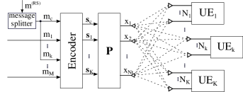
Figure 1: System model.

At the transmitter, a linear precoder $\mathbf{P}^{\left(\text{RS}\right)}=\left[\mathbf{p}_{c},\mathbf{P}\right]\in\mathbb{C}^{N_{T}\times\left(M+1\right)}$ maps the symbols to the transmit antennas. In particular, $\mathbf{p}_{c}\in\mathbb{C}^{N_{t}}$ performs the mapping of the common symbol to the transmit antennas. The private precoder is given by $\mathbf{P}=\left[\mathbf{P}_{1},\mathbf{P}_{2},\dots,\mathbf{P}_{K}\right]$, where $\mathbf{P}_{k}\in\mathbb{C}^{N_{t}\times M_{k}}$ denotes the private precoder of the $k$th user and the vector $\mathbf{p}_{k}$ denotes the $k$th column of $\mathbf{P}$.

Let us consider a general diagonal power loading matrix $\mathbf{A}^{\left(\text{RS}\right)}=\text{diag}\left(\mathbf{a}^{\left(\text{RS}\right)}\right)\in\mathbb{R}^{\left(M+1\right)\times\left(M+1\right)}$. The vector $\mathbf{a}^{\left(\text{RS}\right)}=[a_{c},\mathbf{a}_{1}^{\text{T}},\mathbf{a}_{2}^{\text{T}},\cdots,\mathbf{a}_{k}^{\text{T}}]^{\text{T}}$ assigns the power to the common and private streams. Specifically, the vector $\mathbf{a}_{k}\in\mathbb{R}^{M_{k}}$ allocates the power to the $M_{k}$ private symbols in $\mathcal{M}_{k}$ and the coefficient $a_{c}$ designates the power to the common message. Then, the transmitted signal is expressed by

$$\mathbf{x}=a_{c}s_{c}\mathbf{p}_{c}+\sum_{k=1}^{K}\mathbf{P}_{k}\text{diag}\left(\mathbf{a}_{k}\right)\mathbf{s}_{k}.$$ (1)

The model satisfies the transmit power constraint $\mathbb{E}\left[\lVert\mathbf{x}\rVert^{2}\right]\leq E_{tr}$, where $E_{tr}$ denotes the total transmit power. The transmit vector $\mathbf{x}$ passes through the channel $\mathbf{H}^{\text{T}}=\mathbf{\hat{H}}^{\text{T}}+\mathbf{\tilde{H}}^{\text{T}}\in\mathbb{C}^{N_{r}\times N_{t}}$, where $\mathbf{\hat{H}}^{\text{T}}$ designates the channel estimate and the matrix $\mathbf{\tilde{H}}^{\text{T}}$ models the CSIT quality by adding the estimation error. The matrix $\mathbf{H}_{k}^{\text{T}}\in\mathbb{C}^{N_{k}\times N_{t}}$ represents the channel of the $k$th user. It follows that $\mathbf{H}=[{\mathbf{H}}_{1},\ldots,{\mathbf{H}}_{k},\ldots,{\mathbf{H}}_{K}]$. For simplicity, we consider a flat fading channel which remains fixed during a transmission block.

The signal obtained at the $k$th user following (1) is

$$\mathbf{y}_{k}= \overbrace{a_{c}s_{c}\mathbf{H}_{k}^{\text{T}}\mathbf{p}_{c}}^{\text{Common stream}}+\overbrace{\sum_{i\in\mathcal{M}_{k}}a_{i}s_{i}\mathbf{H}_{k}^{\text{T}}\mathbf{p}_{i}}^{\text{User-k private streams}}+\overbrace{\sum_{\begin{subarray}{c}j=1\\ j\notin\mathcal{M}_{k}\end{subarray}}^{M}a_{j}s_{j}\mathbf{H}_{k}^{\text{T}}\mathbf{p}_{j}}^{\text{Multi-User Interference}}+\mathbf{n}_{k},$$ (2)

where the noise vector $\mathbf{n}_{k}\in\mathbb{C}^{N_{k}\times 1}$ is assumed uncorrelated and follows a complex normal distribution i.e., $\mathbf{n}_{k}\sim\mathcal{CN}\left(\mathbf{0},\sigma_{n}^{2}\mathbf{I}\right)$. The power of (2) at the $i$th receive antenna is given by

$$\mathbb{E}\left[\lvert\text{y}_{k,i}\rvert^{2}\right]= a_{c}^{2}\lvert\mathbf{h}^{\left(k\right)^{\text{T}}}_{i}\mathbf{p}_{c}\rvert^{2}+\sum_{\begin{subarray}{c}j=1\end{subarray}}^{M}a_{j}^{2}\lvert\mathbf{h}^{\left(k\right)^{\text{T}}}_{i}\mathbf{p}_{j}\rvert^{2}+\sigma_{n}^{2}.$$ (3)

Under perfect CSIT assumption, the estimation error goes to zero and equations (2) and (3) remain the same with $\mathbf{H}=\mathbf{\hat{H}}$. Note that the conventional non-RS MIMO system represents a particular case of the model established where no power is distributed to the common message, i.e., $a_{c}=0$ (and therefore no split of the message is conducted).

In what follows we consider the RBD precoding technique [13, 14, 15, 16, 17] to define the private precoder. RBD separates the precoder into two matrices, i.e., $\mathbf{P}_{k}^{\left(\text{RBD}\right)}=\mathbf{P}^{a}_{k}\mathbf{P}^{b}_{k}.$ The filter $\mathbf{P}^{a}_{k}$ partially removes MUI [13] and is computed through the following optimization problem:

$$\mathbf{P}^{a}_{k}=\min_{\mathbf{P}^{a}_{k}}\mathbb{E}\left[\lVert\mathbf{\bar{H}}^{\text{T}}_{k}\mathbf{P}^{a}_{k}\rVert^{2}+\frac{\lVert\mathbf{n}_{k}\rVert^{2}}{\delta^{2}}\right],$$ (4)

where the matrix $\mathbf{\bar{H}}_{k}$ is formed by excluding the $k$th user, i.e. $\mathbf{\bar{H}}_{k}=\left[\mathbf{H}_{1},\ldots,\mathbf{H}_{k-1},~{}\mathbf{H}_{k+1},\ldots,\mathbf{H}_{K}\right]$ and the parameter $\delta$ is a scaling factor imposed in order to fulfil the transmit power constraint. By applying SVD we get $\mathbf{\bar{H}}_{k}^{\text{T}}=\mathbf{\bar{U}}_{k}\mathbf{\bar{\Psi}}_{k}\mathbf{\bar{V}}_{k}^{H}$. The solution to (4) is given by

$$\mathbf{P}^{a}_{k}=\mathbf{\bar{V}}_{k}\left(\mathbf{\bar{\Psi}_{k}}^{\text{T}}\mathbf{\bar{\Psi}}_{k}+\frac{N_{r}\sigma_{n}^{2}}{E_{tr}}\mathbf{I}_{N_{t}}\right)^{-1/2}$$ (5)

The second filter $\mathbf{P}^{b}_{k}$ allows parallel symbol detection. Consider the effective channel matrix defined as $\underaccent{\ddot}{\mathbf{H}}_{k}^{\text{T}}=\mathbf{H}_{k}^{\text{T}}\mathbf{P}^{a}_{k}$. A second SVD is computed on the effective channel , i.e., $\underaccent{\ddot}{\mathbf{H}}_{k}^{\text{T}}=\underaccent{\ddot}{\mathbf{U}}_{k}\underaccent{\ddot}{\mathbf{\Psi}}_{k}\underaccent{\ddot}{\mathbf{V}}_{k}^{H}$, in order to find the second precoder and the receive filter of the $k$th user as given by

$$\mathbf{P}^{b}_{k}= \underaccent{\ddot}{\mathbf{V}}_{k}, \mathbf{G}^{\left(\text{RBD}\right)}_{k}= \underaccent{\ddot}{\mathbf{U}}_{k}^{H}.$$ (6)

III Proposed Stream Combining Techniques

Let us consider a system employing an RS scheme with Gaussian signalling. The instantaneous common rate at the $k$th user is defined as

$$R_{c,k}=\log_{2}\left(1+\gamma_{c,k}\right),$$ (7)

where $\gamma_{c,k}$ is the Signal-to-Interference-plus-noise ratio (SINR) at the $k$th user when decoding the common message.

In order to evaluate the performance we consider the Ergodic Sum Rate (ESR) over a long sequence of fading channel states to ensure that the rates are achievable, as detailed in [3]. The total ESR of the system is given by

$$S_{r}=\min_{k\in\left[1,K\right]}\mathbb{E}\left[\bar{R}_{c,k}\right]+\mathbb{E}\left[\bar{R}_{p}\right].$$ (8)

The first term of (8) represents the ergodic common rate, where $\bar{R}_{c,k}=\mathbb{E}\left[R_{c,k}\lvert\hat{\mathbf{H}}\right]$. The min operator is used since all users should decode the common message. The second term denotes the ergodic sum-private rate with $\bar{R}_{p}=\mathbb{E}\left[R_{p}\lvert\hat{\mathbf{H}}\right]$. The sum-private rate $R_{p}$ embodies all private rates, i.e., $R_{p}=\sum_{k=1}^{K}R_{k}$, where $R_{k}$ denotes the instantaneous private rate of the $k$th user.

Unlike receivers in RS MISO systems, the $k$th receiver in a MIMO system has access to $N_{k}$ copies of the common symbol. Let us consider (2) and define the combined signal $\tilde{\text{y}}_{k}=\mathbf{w}_{k}^{H}\mathbf{y}_{k}$, where the vector $\mathbf{w}_{k}=\left[w_{1}~{}~{}w_{2}~{}~{}\cdots~{}~{}w_{M_{k}}\right]^{\text{T}}$ represents the combining filter used to maximize the SNR. Let us define the vectors $\mathbf{r}_{k,c}=\mathbf{H}_{k}^{\text{T}}\mathbf{p}_{c}$ and $\mathbf{r}_{k,i}=\mathbf{H}_{k}^{\text{T}}\mathbf{p}_{i}$. Then, the average power of $\tilde{\text{y}}_{k}$ is

$$\mathbb{E}\left[\lvert\tilde{\text{y}}_{k}\rvert^{2}\right]=a_{c}^{2}\lvert\mathbf{w}_{k}^{H}\mathbf{r}_{k,c}\rvert^{2}+\sum_{j=1}^{M}a_{j}^{2}\lvert\mathbf{w}_{k}^{H}\mathbf{r}_{k,j}\rvert^{2}+\lVert\mathbf{w}_{k}\rVert^{2}\sigma_{n}^{2}.$$ (9)

From (9) we get the common message SINR given by

$$\gamma_{k,c}=\frac{a_{c}^{2}\lvert\mathbf{w}_{k}^{H}\mathbf{r}_{k,c}\rvert^{2}}{\sum\limits_{i\in\mathcal{M}_{k}}a_{i}^{2}\lvert\mathbf{w}_{k}^{H}\mathbf{r}_{k,i}\rvert^{2}+\sum\limits_{\begin{subarray}{c}j=1\\ j\notin\mathcal{M}_{k}\end{subarray}}^{M}a_{j}^{2}\lvert\mathbf{w}_{k}^{H}\mathbf{r}_{k,j}\rvert^{2}+\lVert\mathbf{w}_{k}\rVert^{2}\sigma_{n}^{2}}.$$ (10)

The structure of the $k$th receiver is shown in Fig. 2, which is different from [11], where the combiner and the private receiver are implemented sequentially. In what follows, we propose combining strategies to set up $\mathbf{w}_{k}$ and enhance the common rate performance.

Figure 2: Receiver structure.

III-A Min-Max Criterion

Let us consider (3) from the model described in (2). The common rate obtained at the $i$th receive antenna of user $k$ can be computed by

$$R_{c,k,i}=\log_{2}\left(1+\frac{a_{c}^{2}\lvert\mathbf{h}_{i}^{\left(k\right)^{\text{T}}}\mathbf{p}_{c}\rvert^{2}}{\sum_{j=1}^{M}a_{j}^{2}\lvert\mathbf{h}_{i}^{\left(k\right)^{\text{T}}}\mathbf{p}_{j}\rvert^{2}+\sigma_{n}^{2}}\right).$$ (11)

The Min-Max criterion selects at each receiver the antenna that leads to the highest common rate, i.e., $R_{c,k}^{\left(\text{max}\right)}=\max_{i}\left(R_{c,k,i}\right).$ The $k$th entry of $\mathbf{w}_{k}$ is set to one if the $k$th antenna is selected and all the other entries are set to zero. Using $R_{c,k}^{\left(\text{max}\right)}$ with (8) we get the sum rate performance.

III-B Maximum Ratio Combining

Another possibility to enhance the common rate is to use Maximum Ratio Combining (MRC). The maximum value of the numerator is achieved when $\mathbf{w}_{k}^{\left(\text{MRC}\right)}=\frac{\mathbf{r}_{k,c}}{\lVert\mathbf{r}_{k,c}\rVert^{2}}$ i.e., when the vectors $\mathbf{w}_{k}$ and $\mathbf{r}_{k,c}$ are parallel. Using the property of the dot product and simplifying terms in (10), the SINR can be expressed as follows:

$$\gamma_{k,c}^{\left(\text{MRC}\right)}=\frac{a_{c}^{2}\lVert\mathbf{r}_{k,c}\rVert^{2}}{\sum\limits_{i\in\mathcal{M}_{k}}a_{i}^{2}\lVert\mathbf{r}_{k,i}\rVert^{2}\cos\beta_{i}+\sum\limits_{\begin{subarray}{c}j=1\\ j\notin\mathcal{M}_{k}\end{subarray}}^{M}a_{j}^{2}\lVert\mathbf{r}_{k,j}\rVert^{2}\cos\beta_{j}+\sigma_{n}^{2}}.$$ (12)

where $\beta_{j}$ is the angle between $\mathbb{w}_{k}$ and $\mathbf{r}_{k,j}$. The sum rate performance can be found by using (12) in (7) and in (8).

III-C Minimum Mean-Square Error Combining

The proposed MMSE combiner (MMSEc) considers the optimization problem given by

$$\mathbf{w}_{k}^{\left(\text{MMSE}\right)}=\min_{\mathbf{w}_{k}}\mathbb{E}\left[\lVert s_{c}-\mathbf{w}_{k}^{H}\mathbf{y}_{k}\rVert^{2}\right].$$ (13)

Evaluating the expected value on the right side of (13), we have

$$\mathbb{E}\left[\lVert s_{c}-\mathbf{w}_{k}^{H}\mathbf{y}_{k}\rVert^{2}\right]= \mathbb{E}\left[\left(s_{c}-\mathbf{w}_{k}^{H}\mathbf{y}_{k}\right)\left(s_{c}-\mathbf{w}_{k}^{H}\mathbf{y}_{k}\right)\right]$$

$$= 1-\mathbf{w}_{k}^{H}\mathbf{H}_{k}^{\text{T}}\mathbf{p}_{c}-\mathbf{p}_{c}^{H}\mathbf{H}_{k}^{*}\mathbf{w}_{k}+$$

$$\mathbf{w}_{k}^{H}\mathbf{R}_{\mathbf{y}_{k}\mathbf{y}_{k}}\mathbf{w}_{k},$$ (14)

where $\mathbf{R}_{\mathbf{y}_{k}\mathbf{y}_{k}}=\mathbb{E}\left[\mathbf{y}_{k}\mathbf{y}_{k}^{H}\right]$. Taking the derivative with respect to $\mathbf{w}_{k}^{H}$ and equating the result to zero we obtain

$$\frac{\partial\mathbb{E}\left[\lVert s_{c}-\mathbf{w}_{k}^{H}\mathbf{y}_{k}\rVert^{2}\right]}{\partial\mathbf{w}_{k}^{H}}=-\mathbf{H}_{k}^{\text{T}}\mathbf{p}_{c}+\mathbf{R}_{\mathbf{y}_{k}\mathbf{y}_{k}}\mathbf{w}_{k}=0.$$ (15)

Solving (15) with respect to $\mathbf{w}_{k}$ we get the MMSEc expression, which is given by

$$\mathbf{w}_{k}^{\left(\text{MMSE}\right)}=\mathbf{R}_{\mathbf{y}_{k}\mathbf{y}_{k}}^{-1}\mathbf{H}_{k}\mathbf{p}_{c}.$$ (16)

Let us consider the quantities:

$$\lVert\mathbf{w}_{k}\rVert^{2}\sigma_{n}^{2}=\text{tr}\left(\mathbf{R}_{\mathbf{y}_{k}\mathbf{y}_{k}}^{-2}\mathbf{H}_{k}^{\text{T}}\mathbf{p}_{c}\mathbf{p}_{c}^{H}\mathbf{H}_{k}^{*}\right)\sigma_{n}^{2},$$ (17)

$$\lvert\mathbf{w}_{k}^{H}\mathbf{r}_{k,i}\rvert^{2}=\mathbf{p}_{i}^{H}\mathbf{H}_{k}^{*}\mathbf{R}_{\mathbf{y}_{k}\mathbf{y}_{k}}^{-1}\mathbf{H}_{k}^{\text{T}}\mathbf{p}_{c}\mathbf{p}_{c}^{H}\mathbf{H}_{k}^{*}\mathbf{R}_{\mathbf{y}_{k}\mathbf{y}_{k}}^{-1}\mathbf{H}_{k}^{\text{T}}\mathbf{p}_{i},$$ (18)

$$\lvert\mathbf{w}_{k}^{H}\mathbf{r}_{k,c}\rvert^{2}=\mathbf{p}_{c}^{H}\mathbf{H}_{k}^{*}\mathbf{R}_{\mathbf{y}_{k}\mathbf{y}_{k}}^{-1}\mathbf{H}_{k}^{\text{T}}\mathbf{p}_{c}\mathbf{p}_{c}^{H}\mathbf{H}_{k}^{*}\mathbf{R}_{\mathbf{y}_{k}\mathbf{y}_{k}}^{-1}\mathbf{H}_{k}^{\text{T}}\mathbf{p}_{c},$$ (19)

Substituting (17),(18), and (19) into (10) we obtain the SINR of MMSEc, which can be used with (7) to get the common rate.

III-D Private Rate

The common symbol is removed from the received signal using a SIC technique [18, 19, 20, 21, 22, 23]. A receive filter $\mathbf{G}_{k}\in\mathbb{C}^{M_{k}\times N_{k}}$ can be used to improve the detection of the private symbols. Let us consider the matrix $\mathbf{F}_{k}=\mathbf{G}_{k}\mathbf{H}_{k}^{\text{T}}$ in order to simplify the notation. Then, the achievable rate of the $k$th user is described by

$$R_{k}=\log_{2}\left(\det\left[\mathbf{I}+\mathbf{F}_{k}\mathbf{P}_{k}\text{diag}\left(\mathbf{a}_{k}\odot\mathbf{a}_{k}\right)\mathbf{P}_{k}^{H}\mathbf{F}^{H}_{k}\mathbf{R}_{\mathbf{z}_{k}\mathbf{z}_{k}}^{-1}\right]\right),$$ (20)

where the covariance matrix of the effective noise is given by

$$\mathbf{R}_{\mathbf{z}_{k}\mathbf{z}_{k}}=\sum\limits_{\begin{subarray}{c}i=1\\ i\neq k\end{subarray}}^{K}\mathbf{F}_{k}\mathbf{P}_{i}\text{diag}\left(\mathbf{a}_{i}\odot\mathbf{a}_{i}\right)\mathbf{P}_{i}^{H}\mathbf{F}_{k}^{H}+\sigma_{n}^{2}\mathbf{I}.$$ (21)

IV Rate Analysis

In this section, we carry out the sum rate analysis of the proposed strategies combined with the RBD precoder. Let us consider the matrices $\mathbf{H}^{\left(k,j\right)}=\mathbf{H}_{k}^{\text{T}}\mathbf{P}^{a}_{j}$,$\mathbf{\Upsilon}^{\left(k,j\right)}=\underaccent{\ddot}{\mathbf{U}}_{k}^{H}\mathbf{H}^{\left(k,j\right)}\underaccent{\ddot}{\mathbf{V}}_{j}$ and $\mathbf{\tilde{\Upsilon}}^{\left(k,j\right)}=\underaccent{\ddot}{\mathbf{U}}_{k}^{H}\mathbf{\tilde{H}}^{\left(k,j\right)}\underaccent{\ddot}{\mathbf{V}}_{j}$ . Employing an RBD precoder leads us to the following received vector:

$$\mathbf{y}_{k}= a_{c}s_{c}\mathbf{H}_{k}^{\text{T}}\mathbf{p}_{c}+\left(\underaccent{\ddot}{\mathbf{U}}_{k}\underaccent{\ddot}{\mathbf{\Psi}}_{k}+\mathbf{\tilde{\Upsilon}}^{\left(k,k\right)}\right)\text{diag}\left(\mathbf{a}_{k}\right)\mathbf{s}_{k}$$

$$+\sum\limits_{\begin{subarray}{c}j=1\\ j\neq k\end{subarray}}^{K}\mathbf{\Upsilon}^{\left(k,j\right)}\text{diag}\left(\mathbf{a}_{j}\right)\mathbf{s}_{j}+\underaccent{\ddot}{\mathbf{U}}_{k}^{H}\mathbf{n}_{k}$$ (22)

For the Min-Max criterion, we have

$$R_{c,k,i}^{\left(RBD\right)}=\log_{2}\Bigg{(}1+\frac{a_{c}^{2}\lvert\mathbf{h}^{\left(k\right)^{\text{T}}}_{j}\mathbf{p}_{c}\rvert^{2}}{\rho^{\left(\text{RBD}\right)^{2}}_{i,k}+{\sum\limits_{\begin{subarray}{c}j=1\\ j\neq k\end{subarray}}^{K}\sum\limits_{m\in\mathcal{M}_{j}}a_{m}^{2}\lvert\upsilon^{\left(k,j\right)}_{i,m-n_{j}}\rvert^{2}}+\sigma_{n}^{2}}\Bigg{)},$$ (23)

where $\rho_{i,k}^{\left(\text{RBD}\right)^{2}}=\sum\limits_{\begin{subarray}{c}l\in\mathcal{M}_{k}\end{subarray}}a_{l}^{2}\lvert\psi_{l-n_{k}}^{\left(k\right)}u_{i,l-n_{k}}^{\left(k\right)}+\tilde{\upsilon}^{\left(k,k\right)}_{i,l-n_{k}}\rvert^{2}$. Then we set $R_{c,k}^{\left(\text{max}\right)}=\max_{i}R_{c,k,i}^{\left(RBD\right)}$ and use (7) and (8) to obtain the performance of the Min-Max criterion. In a perfect CSIT scenario, we have $\mathbf{\Upsilon}^{\left(k,j\right)}=\mathbf{\hat{\Upsilon}}^{\left(k,j\right)}$ and $R_{c,k,i}^{\left(RBD\right)}$ is given by (23) with $\rho_{i,k}^{\left(\text{RBD}\right)^{2}}=\sum\limits_{\begin{subarray}{c}l\in\mathcal{M}_{k}\end{subarray}}a_{l}^{2}\lvert\psi_{l-n_{k}}^{\left(k\right)}u_{i,l-n_{k}}^{\left(k\right)}+\hat{\upsilon}^{\left(k,k\right)}_{i,l-n_{j}k}\rvert^{2}$.

Let us now consider MRC for the $k$th user and evaluate the vector $\mathbf{r}_{k,j}$ with $j\in\mathcal{M}_{q}$ and the column index $t=j-n_{q}$. When $q=k$ the squared norm of vector $\mathbf{r}_{k,j}$ is reduced to:

$$\lVert\mathbf{r}_{k,j}\rVert^{2}=\lVert\underaccent{\ddot}{\psi}_{t}^{\left(k\right)}\underaccent{\ddot}{\mathbf{u}}^{\left(k\right)}_{t}+\underaccent{\ddot}{\mathbf{\tilde{H}}}_{k}^{\text{T}}\underaccent{\ddot}{\mathbf{v}}^{\left(k\right)}_{t}\rVert^{2}.$$ (24)

When $q\neq k$ the squared norm of $\mathbf{r}_{k,j}$ is given by

$$\lVert\mathbf{r}_{k,j}\rVert^{2}=E_{tr}\sum_{i=1}^{N_{k}}\left\lvert\sum_{l=1}^{N_{t}}\sum_{n=1}^{N_{t}}h_{i,l}^{\left(k\right)}\lambda_{n}^{\left(q\right)}\bar{v}_{l,n}^{\left(q\right)}\underaccent{\ddot}{v}_{n,t}^{\left(q\right)}\right\rvert^{2},$$ (25)

where $\lambda_{n}^{\left(q\right)}=\left(\sqrt{E_{tr}\psi_{n}^{\left(q\right)}+N_{r}\sigma_{n}^{2}}\right)^{-1}$. Substituting (24) and (25) in (12) we get the SINR of the MRC criterion, which can be used in (7) and (8) to obtain the achievable sum rate. Under perfect CSIT assumption, (24) is reduced to $\lVert\mathbf{r}_{k,j}\rVert^{2}=\lvert\underaccent{\ddot}{\psi}_{t}^{\left(k\right)}\rvert^{2}$.

Finally, we consider MMSEc and define $\mathbf{D}_{k}=\underaccent{\ddot}{\mathbf{U}}_{k}\underaccent{\ddot}{\mathbf{\Psi}}_{k}+\mathbf{\tilde{\Upsilon}}^{\left(k,k\right)}$, $\mathbf{J_{k}}=\text{diag}\left(\mathbf{a}_{k}\odot\mathbf{a}_{k}\right)$. In the case of MMSEc, we have

$$\small\sum\limits_{i\in\mathcal{M}_{k}}a_{i}^{2}\lvert\mathbf{w}_{k}^{H}\mathbf{r}_{k,i}\rvert^{2}=\text{tr}\left(\mathbf{r}_{k,c}^{H}\mathbf{R}_{\mathbf{y}_{k}\mathbf{y_{k}}}^{-1}\mathbf{D}_{k}\mathbf{J}_{k}\mathbf{D}_{k}^{H}\mathbf{R}_{\mathbf{y}_{k}\mathbf{y_{k}}}^{-1}\mathbf{r}_{k,c}\right)$$ (26)

$$\small\sum\limits_{\begin{subarray}{c}j=1\\ j\notin\mathcal{M}_{k}\end{subarray}}^{M}a_{j}^{2}\lvert\mathbf{w}_{k}^{H}\mathbf{r}_{k,j}\rvert^{2}=\sum\limits_{\begin{subarray}{c}j=1\\ j\neq k\end{subarray}}^{K}\text{tr}\left(\mathbf{r}_{k,c}^{H}\mathbf{R}_{\mathbf{y}_{k}\mathbf{y}_{k}}^{-1}\mathbf{\tilde{\Upsilon}}^{\left(k,j\right)}\mathbf{J}_{k}\mathbf{\tilde{\Upsilon}}^{\left(k,j\right)^{H}}\mathbf{R}_{\mathbf{y}_{k}\mathbf{y_{k}}}^{-1}\mathbf{r}_{k,c}\right)$$ (27)

Substituting (26) and (27) in (10) we obtain the SINR, which can be used in (7) and (8) to obtain the sum rate.

V Simulations

In this section we evaluate the performance of the proposed combining techniques in a RS-based MIMO system employing MMSE and RBD precoders. As reported in the literature [1, 13], these precoders outperform their ZF and BD counterparts by allowing small MUI to significantly reduce the power penalty associated with linear precoding. We set $\mathbf{G}_{k}=\mathbf{I}$ for the MMSE precoder, whereas the RBD precoder uses the receiver defined in (6) since we focus on evaluating the common combiners. We consider $N_{t}=12$ and $K=6$ for all simulations. Each user is equipped with 2 receive antennas. The inputs are Gaussian distributed with zero mean and unit variance. Each coefficient of $\tilde{\mathbf{H}}$ follows a Gaussian distribution, i.e., $\sim\mathcal{CN}(0,\sigma^{2}_{e})$. We consider additive white Gaussian noise and define $\text{SNR}\triangleq E_{tr}/\sigma_{n}^{2}$ with $\sigma_{n}^{2}=1$ for all simulations. The ESR was computed averaging 1000 independent channel realizations. For each channel realization we obtained $\bar{R}_{c}$ and $\bar{R}_{p}$ employing 100 error matrices. We use SVD over the channel $\left(\mathbf{H}=\mathbf{U}\mathbf{\Psi}\mathbf{V}\right)$ and then set $\mathbf{p}_{c}=\mathbf{v}_{1}$. The power allocated to $s_{c}$ was found through exhaustive search in order to maximize the sum rate. Uniform power allocation is used across private users.

For the first simulation, we fixed the channel error variance to $\sigma_{e}^{2}=0.1$. Fig. 3 shows the sum-private rate and the common rate of the RBD precoder with MMSEc, denoted by RBD-RS-MMSEc-Pr and RBD-RS-MMSEc-Cr respectively. The sum-private rate decreases up to 6% when compared to the conventional RBD precoding since part of the transmit power is allocated to the common stream. However, the common rate attains up to 20% of the conventional RBD rate, leading to an overall gain of the system performance. It is important to note that to obtain the gain an efficient power allocation scheme between common and private streams should be employed. The RS scheme deals partially with the MUI which is shown in Fig. 3 where the common rate increases as the SNR grows.

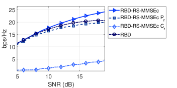
Figure 3: Sum Rate performance under imperfect CSIT

Fig. 4 shows the performance of the proposed schemes as the estimation error increases. The conventional precoders are denoted by MMSE and RBD. MMSE-RS and RBD-RS denote the RS scheme without the common combiner. The best strategy from [11] is represented by BD-RS-MRC. For this simulation we set the SNR to $20$ dB. The robustness of the system increases across all error variances when a common combiner is employed as shown in Fig. 4. The figure shows that the proposed strategy outperforms the BD-RS-MRC scheme. The proposed MIMO RBD-RS-MMSEc attains a sum rate performance up to 34% higher than conventional RBD. Moreover, MMSEc achieves the best performance among the combiners.

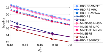
Figure 4: Error variance VS Sum Rate performance

In the last example, we consider that the error in the channel estimate is reduced as the SNR increases, i.e. $\sigma^{2}_{e}=\xi\left(E_{tr}/\sigma^{2}_{n}\right)^{-\alpha}$ with $\xi=0.94$ and $\alpha=0.6$. Fig. 5 shows that the use of combiners results in a higher sum rate than that of conventional schemes. The proposed MIMO RBD-RS-MMSEc obtains the best performance, which is up to 15% when compared to conventional RBD precoding. Future work might consider massive MIMO systems [24, 25]

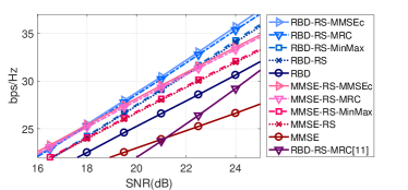
Figure 5: Sum rate performance with imperfect CSIT.

VI Conclusion

Simulation results show that employing a common stream significantly increase the overall performance of the system, contributing up to 20% to the overall system sum rate. Furthermore, the proposed common stream combiners exploit the multipath propagation and the multiple antennas at the receiver to enhancing even more the performance of the common rate as shown by the simulations. The RBD-RS-MMSEc shows an increase in the sum rate performance of more than 15% when compared to conventional techniques. MMSEc also obtains the best performance among the combiners. Simulations have shown that the proposed stream combiners increase the robustness of the system under imperfect CSIT.

References

• [1] M. Joham, W. Utschick, and J. A. Nossek, “Linear transmit processing in MIMO communications systems,” IEEE Transactions on Signal Processing, vol. 53, no. 8, pp. 2700–2712, Aug. 2005.
• [2] Q. H. Spencer, A. L. Swindlehurst, and M. Haardt, “Zero-forcing methods for downlink spatial multiplexing in multiuser MIMO channels,” IEEE Transactions on Signal Processing, vol. 52, no. 2, pp. 461–471, Feb. 2004.
• [3] H. Joudeh and B. Clerckx, “Sum-rate maximization for linearly precoded downlink multiuser MISO systems with partial CSIT: A rate-splitting approach,” IEEE Transactions on Communications, vol. 64, no. 11, pp. 4847–4861, Nov. 2016.
• [4] B. Clerckx, H. Joudeh, C. Hao, M. Dai, and B. Rassouli, “Rate splitting for MIMO wireless networks: a promising PHY-layer strategy for LTE evolution,” IEEE Communications Magazine, vol. 54, no. 5, pp. 98–105, May 2016.
• [5] Y. Mao, B. Clerckx, and V. Li, “Rate-splitting multiple access for downlink communication systems: Bridging, generalizing and outperforming SDMA and NOMA,” EURASIP Journal on Wireless Communications and Networking, vol. 2018, no. 1, p. 133, May 2018.
• [6] C. Hao, Y. Wu, and B. Clerckx, “Rate analysis of two-receiver MISO broadcast channel with finite rate feedback: A rate-splitting approach,” IEEE Transactions on Communications, vol. 63, no. 9, pp. 3232–3246, Sep. 2015.
• [7] A. R. Flores, B. Clerckx, and R. C. de Lamare, “Tomlinson-Harashima precoded rate-splitting for multiuser multiple-antenna systems,” in 2018 15th International Symposium on Wireless Communication Systems (ISWCS), Lisbon, 2018.
• [8] H. Joudeh and B. Clerckx, “Robust transmission in downlink multiuser MISO systems: A rate-splitting approach,” IEEE Transactions on Signal Processing, vol. 64, no. 23, pp. 6227–6242, Dec. 2016.
• [9] G. Lu, L. Li, H. Tian, and F. Qian, “MMSE-based precoding for rate splitting systems with finite feedback,” IEEE Communications Letters, vol. 22, no. 3, pp. 642–645, Mar. 2018.
• [10] C. Hao, B. Rassouli, and B. Clerckx, “Achievable DoF regions of MIMO networks with imperfect CSIT,” IEEE Transactions on Information Theory, vol. 63, no. 10, pp. 6587–6606, Oct. 2017.
• [11] A. Flores and R. C. de Lamare, “Linearly precoded rate-splitting techniques with block diagonalization for multiuser MIMO systems,” in 2019 IEEE International Conference on Communications Workshops (ICC Workshops), Shanghai, China, 2019.
• [12] A. R. Flores, R. C. De Lamare, and B. Clerckx, “Linear precoding and stream combining for rate splitting in multiuser mimo systems,” IEEE Communications Letters, pp. 1–1, 2020.
• [13] V. Stankovic and M. Haardt, “Generalized design of multi-user MIMO precoding matrices,” IEEE Transactions on Wireless Communications, vol. 7, no. 3, pp. 953–961, Mar. 2008.
• [14] H. Sung, S. . Lee, and I. Lee, “Generalized channel inversion methods for multiuser MIMO systems,” IEEE Transactions on Communications, vol. 57, no. 11, pp. 3489–3499, Nov. 2009.
• [15] K. Zu and R. C. d. Lamare, “Low-complexity lattice reduction-aided regularized block diagonalization for mu-mimo systems,” IEEE Communications Letters, vol. 16, no. 6, pp. 925–928, June 2012.
• [16] K. Zu, R. C. de Lamare, and M. Haardt, “Generalized design of low-complexity block diagonalization type precoding algorithms for multiuser mimo systems,” IEEE Transactions on Communications, vol. 61, no. 10, pp. 4232–4242, October 2013.
• [17] W. Zhang, R. C. de Lamare, C. Pan, M. Chen, J. Dai, B. Wu, and X. Bao, “Widely linear precoding for large-scale mimo with iqi: Algorithms and performance analysis,” IEEE Transactions on Wireless Communications, vol. 16, no. 5, pp. 3298–3312, May 2017.
• [18] R. C. De Lamare and R. Sampaio-Neto, “Minimum mean-squared error iterative successive parallel arbitrated decision feedback detectors for ds-cdma systems,” IEEE Transactions on Communications, vol. 56, no. 5, pp. 778–789, May 2008.
• [19] P. Li, R. C. de Lamare, and R. Fa, “Multiple feedback successive interference cancellation detection for multiuser mimo systems,” IEEE Transactions on Wireless Communications, vol. 10, no. 8, pp. 2434–2439, August 2011.
• [20] R. C. de Lamare and R. Sampaio-Neto, “Adaptive reduced-rank equalization algorithms based on alternating optimization design techniques for mimo systems,” IEEE Transactions on Vehicular Technology, vol. 60, no. 6, pp. 2482–2494, July 2011.
• [21] P. Li and R. C. De Lamare, “Adaptive decision-feedback detection with constellation constraints for mimo systems,” IEEE Transactions on Vehicular Technology, vol. 61, no. 2, pp. 853–859, Feb 2012.
• [22] R. C. de Lamare, “Adaptive and iterative multi-branch mmse decision feedback detection algorithms for multi-antenna systems,” IEEE Transactions on Wireless Communications, vol. 12, no. 10, pp. 5294–5308, October 2013.
• [23] A. G. D. Uchoa, C. T. Healy, and R. C. de Lamare, “Iterative detection and decoding algorithms for mimo systems in block-fading channels using ldpc codes,” IEEE Transactions on Vehicular Technology, vol. 65, no. 4, pp. 2735–2741, April 2016.
• [24] R. C. de Lamare, “Massive mimo systems: Signal processing challenges and future trends,” URSI Radio Science Bulletin, vol. 2013, no. 347, pp. 8–20, Dec 2013.
• [25] W. Zhang, H. Ren, C. Pan, M. Chen, R. C. de Lamare, B. Du, and J. Dai, “Large-scale antenna systems with ul/dl hardware mismatch: Achievable rates analysis and calibration,” IEEE Transactions on Communications, vol. 63, no. 4, pp. 1216–1229, April 2015.