Photon-Mediated Charge Exchange Reactions Between ³⁹K Atoms and ⁴⁰Ca⁺ Ions in a Hybrid Trap

Abstract

We present experimental evidence of charge exchange between laser-cooled potassium ³⁹K atoms and calcium ⁴⁰Ca⁺ ions in a hybrid atom-ion trap and give quantitative theoretical explanations for the observations. The ³⁹K atoms and ⁴⁰Ca⁺ ions are held in a magneto-optical (MOT) and a linear Paul trap, respectively. Fluorescence detection and high resolution time of flight mass spectra for both species are used to determine the remaining number of ⁴⁰Ca⁺ ions, the increasing number of ³⁹K⁺ ions, and ³⁹K number density as functions of time. Simultaneous trap operation is guaranteed by alternating periods of MOT and ⁴⁰Ca⁺ cooling lights, thus avoiding direct ionization of ³⁹K by the ⁴⁰Ca⁺ cooling light. We show that the K-Ca⁺ charge-exchange rate coefficient increases linearly from zero with ³⁹K number density and the fraction of ⁴⁰Ca⁺ ions in the 4p ²P_1/2 electronically-excited state. Combined with our theoretical analysis, we conclude that these data can only be explained by a process that starts with a potassium atom in its electronic ground state and a calcium ion in its excited 4p ²P_1/2 state producing ground-state ³⁹K⁺ ions and metastable, neutral Ca (3d4p³P₁) atoms, releasing only 150 cm^-1 equivalent relative kinetic energy. Charge-exchange between either ground- or excited-state ³⁹K and ground-state ⁴⁰Ca⁺ is negligibly small as no energetically-favorable product states are available. Our experimental and theoretical rate coefficients are in agreement given the uncertainty budgets.

I Introduction

Over the past few decades, laser cooling and trapping of atoms, ions, and molecules have significantly contributed to advancing fundamental atomic, molecular, and optical physics research. More recently, experiments successfully merged ion and neutral atom trapping techniques. These experiments include the study of reaction dynamics of neutral atoms and atomic ions Grier et al. (2009); Zipkes et al. (2010); Schmid et al. (2010); Hall et al. (2011); Rellergert et al. (2011); Härter et al. (2012); Ravi et al. (2012); Sivarajah et al. (2012); Ray et al. (2014); Smith et al. (2014); Goodman et al. ; Meir et al. (2016); Saito et al. (2017); Joger et al. (2017); Sikorsky et al. (2018); Kwolek et al. (2019); Tomza et al. (2019), as well as of cold atoms and molecular ionsHall and Willitsch (2012); Deiglmayr et al. (2012); Sullivan et al. (2012); Rellergert et al. (2013). Here, the long storage times of laser-cooled ion-atom systems has allowed the study of processes that are difficult to observe otherwise. The internal and external states of the atoms and ions can be manipulated using laser fields, which enables a careful investigation of the quantum-state dependence of a process.

Most research has focused on colliding neutral and ionic atoms or molecules prepared in their electronic ground state. When one or both colliding partners, however, are prepared in excited electronic states more inelastic channels become available and richer dynamics occurs with corresponding challenges in the theoretical interpretation. Recently, such inelastic collisions have been reported for the ion in an excited state Staanum et al. (2004); Hall et al. (2011); Ratschbacher et al. (2012); Saito et al. (2017); Kwolek et al. (2019); Ben-Shlomi et al. (2019) and for the excited atom colliding with an ion or a charged molecule Mills et al. (2019); Li et al. (2019); Kwolek et al. (2019); Puri et al. (2019); Dörfler et al. (2019), or both particles in an excited state Kwolek et al. (2019). In all these studies the role of excitation in collisional dynamics of various atomic and ionic species has been investigated. However, the control of reaction pathways and population of the excited states is also critically important for multiple applications of ions such as optical frequency standards, quantum simulation, quantum computing and astronomy Schmidt-Kaler et al. (2003); Margolis et al. (2004); Kreuter et al. (2005); Häffner et al. (2008); Blatt and Roos (2012).

Here, we report on the theoretical and experimental investigation of cold charge exchange collisions between laser-cooled potassium (³⁹K) atoms and calcium (⁴⁰Ca⁺) ions in the ground and excited states under controlled experimental conditions. The nearly-equal masses of potassium and calcium enables the simultaneous trapping of the reactant and resultant ions in the same ion trap. Further, direct detection of the ions using a high-resolution time-of-flight mass spectrometer (TOFMS) allows us to follow charge exchange as a function of time. We also show that our data are explained by a process that starts with a potassium atom in its electronic ground state and a calcium ion in its excited 4p ²P_1/2 state producing ground-state ³⁹K⁺ ions and metastable, neutral Ca (4s4p³P₁) atoms, releasing only 150 cm^-1 equivalent relative kinetic energy. Our measured charge-exchange rate coefficient is in good agreement with the theoretical estimate.

The article is organized as follows. In section II, we describe the experimental setup and measurements of the charge-exchange rate coefficient. The theoretical models for different charge exchange pathways are detailed in section III, followed by a discussion in section IV. Details of our electronic structure calculation is given in Supplemental Material.

II Experimental Setup and Observations

The experiments are performed in a spatially overlapped ion-atom hybrid trap comprised of a magneto optical trap (MOT) for neutral ³⁹K atoms and a linear Paul trap for ⁴⁰Ca⁺ ions Jyothi et al. (2019). A schematic of the experimental setup is shown in Fig. 1(a). The ion trap is a segmented electrode linear quadrupole trap with four central rf electrodes (driven at 1.7 MHz) for radial trapping and eight end cap dc electrodes for axial trapping. The apparatus is integrated with a high-resolution TOFMS consisting of two Einzel lenses for ion collimation and a microchannel plate for ion detection.The ions are radially extracted from the Paul trap towards the detector by turning off the rf voltages while, simultaneously, applying high dc voltages on the central electrodes to create a potential gradient.

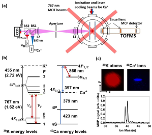
Figure 1: (a) Top view of the experimental apparatus illustrating laser setups, fluorescence detection, and ion time of flight detection. (b) the relevant states, energy levels, and laser colors (not to scale) of ³⁹K, ³⁹K⁺, ⁴⁰Ca, and ⁴⁰Ca⁺. Red vertical lines with arrows and labels $\nu_{\rm c}$ and $\nu_{\rm r}$ correspond to the cooling and repumper lasers for ³⁹K, respectively. The four lasers (blue and red lines with arrows) that control neutral ⁴⁰Ca and ionic ⁴⁰Ca⁺ are discussed in the text. (c) CCD images of the ³⁹K MOT and ⁴⁰Ca⁺ ions, and a TOF mass spectrum showing both ³⁹K⁺ and ⁴⁰Ca⁺ ion peaks.

Neutral ³⁹K atoms derived from a potassium ampule are cooled and trapped in a MOT using three mutually orthogonal and retro-reflected laser beams. The energy-level diagram of ³⁹K atoms relevant for our experiments is shown in Fig. 1(b). Cooling and repumper beams are derived from the same 767 nm laser by MOGLabs mog locked to the D2 crossover peak of a saturation absorption spectrum. A pair of acousto-optic modulators (AOMs) are used to set the desired detunings for the cooling (20 MHz to the red of the 4s($F=2$) to 4p($F’=3$) transition) and repumper (12 MHz to the red of the $F=1$ to $F’=2$ transition) beams. The quadrupole magnetic field for the MOT is created by a pair of coils in anti-Helmholtz configuration mounted outside the vacuum chamber.

Neutral calcium atoms are produced by heating a calcium dispenser with a current of about 2.7 A. The ⁴⁰Ca atoms are ionized by two-photon ionization using lasers at wavelengths of 423 nm and 379 nm focused at the center of the ion trap. The ⁴⁰Ca⁺ ions are Doppler cooled using a 397 nm laser and repumped with an 866 nm laser. The relevant states and energy levels of ⁴⁰Ca and ⁴⁰Ca⁺ are shown in Fig. 1(b). All laser beams for ⁴⁰Ca⁺ are derived from a multi-diode laser module from Toptica Photonics top .

To study cold interactions between ³⁹K and ⁴⁰Ca⁺, the centers of the MOT and Paul trap must coincide. Optimization of the trap overlap is achieved by either moving the MOT center by changing the currents through the coil pair or by moving the center of the Paul trap by changing the dc voltages on the ion trap electrodes. The quality of the relative positioning of the trap centers has been presented in detail in Jyothi et al. (2019). For stable co-trapping and cooling of ³⁹K and ⁴⁰Ca⁺, the 767 nm and 397 nm laser beams are alternately switched at a frequency of 2 kHz using AOMs Jyothi et al. (2019). This prevents ionization of potassium atoms in the MOT from the 4P_3/2 state by the 397 nm Ca⁺ cooling laser beam and limits the reactants collision channels to K(S)+Ca⁺(P), K(P)+Ca⁺(S), and K(S)+Ca⁺(S).

Fluorescence from ³⁹K and ⁴⁰Ca⁺ is detected using photo multiplier tubes (PMT) and an EM-CCD camera. The ³⁹K number density is determined from the fluorescence signal. Ions are also detected using TOFMS, enabling the direct observation of non-fluorescing reaction products such as the ³⁹K⁺ ions. With the optimal extraction voltages, a mass resolution $m/\Delta m$ of 208 is achieved, which is sufficient to resolve the ⁴⁰Ca⁺ and ³⁹K⁺ ion peaks. EM-CCD images of ³⁹K and ⁴⁰Ca⁺ ions as well as a representative TOF mass spectrum of ³⁹K⁺ and ⁴⁰Ca⁺ ions are shown in Fig. 1(c).

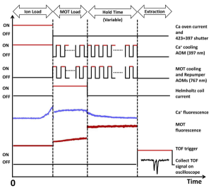
Figure 2: Experimental control sequence to measure the charge-exchange rate between ³⁹K and ⁴⁰Ca⁺ as described in the text. Since the 767 nm and 397 nm laser beams are never simultaneously turned on, excited ³⁹K and excited ⁴⁰Ca⁺ are not simultaneously present. Consequently, charge-exchange collisions only occur via the K(S)+Ca⁺(P), K(P)+Ca⁺(S), and K(S)+Ca⁺(S) channels.

The experiment is controlled by a Kasli FPGA and programmed using ARTIQ (Advanced Real-Time Infrastructure for Quantum physics) Bourdeauducq et al. (2018); art ; Jyothi et al. (2019) provided by m-labs. A typical experimental sequence to measure ³⁹K-⁴⁰Ca⁺ charge exchange is shown in Fig. 2. First, we load and cool approximately 1000 ⁴⁰Ca⁺ into the ion trap. The photo-ionizing lasers for calcium are then blocked using a mechanical shutter to avoid ionization of ³⁹K atoms by these lasers. The MOT laser beams are now turned on to load the MOT to saturation. While loading the MOT, currents on an additional pair of magnetic coils in Helmholtz configuration are turned on to shift the MOT magnetic-field center a few mm from the center of the ion trap. This avoids any interaction between ³⁹K and ⁴⁰Ca⁺ during the MOT loading process. The MOT center is then moved back to the ion-trap center by turning off the Helmholtz coil current. The ³⁹K atoms and ⁴⁰Ca⁺ ions are then allowed to interact for different hold times. During the hold time, the 767 nm and 397 nm laser beams are never on at the same time.

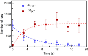
Figure 3: The number of ⁴⁰Ca⁺ and ³⁹K⁺ ions as functions of time for which the ⁴⁰Ca⁺ ions and ³⁹K atoms are held together. Error bars are one standard deviation uncertainties based on six measurements. Dashed lines are exponential fits to the data. The ³⁹K number density in the MOT is $10^{9}$ atoms/cm³.

Figure 4: Typical fluorescence data from ⁴⁰Ca⁺ ions as functions of time in the absence and presence of ³⁹K atoms in the MOT. Blue circles correspond to ⁴⁰Ca⁺ fluorescence data in the absence of the neutral atoms. Purple, red and orange circles show ⁴⁰Ca⁺ fluorescence when the ions are held together with ³⁹K atoms with number densities of $6.8\times 10^{8}$, $14.5\times 10^{8}$, and $16.6\times 10^{8}$, respectively. Dashed lines are exponential fits to the data.

The TOFMS signal, collected as a function of hold time, provides evidence of charge exchange, because our Paul trap holds ⁴⁰Ca⁺ and ³⁹K⁺ ions equally well due to their comparable masses. That is, product ³⁹K⁺ ions are trapped and can be detected with TOFMS. Figure 3 shows the detected number of ⁴⁰Ca⁺ and ³⁹K⁺ ions as a function of hold time. The number of ⁴⁰Ca⁺ decreases with time with a simultaneous one-to-one increase in the number of ³⁹K⁺ ions.

Figure 4 shows typical ⁴⁰Ca⁺ fluorescence as a function of hold time in the absence and presence of ³⁹K atoms. Without ³⁹K atoms, the number of trapped, laser-cooled ⁴⁰Ca⁺ ions is constant for several minutes. When ⁴⁰Ca⁺ ions are allowed to interact with ³⁹K atoms, however, the ⁴⁰Ca⁺ ions disappear in a few seconds as a result of charge exchange. Decay rates measured by ⁴⁰Ca⁺ fluorescence and TOFMS data are consistent. As TOFMS is destructive, both ion and atom traps need to be reloaded for each hold time. Hence, for most measurements described in this article ⁴⁰Ca⁺ ion fluorescence is used to measure decay rates. In fact, fluorescence has been the preferred measurement tool of ultra-cold chemical reaction rates Grier et al. (2009); Hall et al. (2011); Rellergert et al. (2011); Haze et al. (2015).

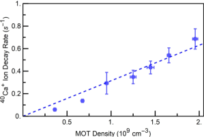
Figure 5: Loss rate of ⁴⁰Ca⁺ ions in the presence of its 397-nm cooling light as a function of ³⁹K number density in the MOT. A linear fit to the data assuming no charge exchange when there are no ³⁹K atoms present gives a rate coefficient of $(4.0\pm{0.2})\times 10^{-10}$ cm³/s. The detuning of the 397-nm laser that cools ⁴⁰Ca⁺ is such that the excited-state ⁴⁰Ca⁺(²P_1/2) population is 24 %.

Figure 5 shows the rate of charge exchange as a function of ³⁹K number density in a MOT when the fraction of ⁴⁰Ca⁺ ions in the excited ²P_1/2 state is 0.24. This excited-state fraction is controlled by the frequency detuning of the 397-nm ⁴⁰Ca⁺ cooling laser from the 4S to 4P_1/2 transition. The rate coefficient increases with ³⁹K number density and a linear fit assuming no charge exchange at zero ³⁹K number density gives a rate coefficient of $(4.0\pm{0.2})\times 10^{-10}$ cm³/s.

To examine the effect of the excited electronic state of ⁴⁰Ca⁺ ions on charge exchange, we varied the population in the 4P_1/2 state by adjusting the frequency detuning and intensity of the ⁴⁰Ca⁺ lasers. Figure 6 shows these data. The rate coefficients increases linearly with excited-state population. We can elaborate that for the 100% population of Ca⁺ ions in the ${}^{2}P$ state the KCa⁺ rate coefficient reaches value of $1.9\times 10^{-9}$ cm³/s, which is only 0.55 times smaller than the Langevin rate for this system (K_L=$3.46\times 10^{-9}$ cm³/s) Langevin (1905) . The rate coefficients of the charge exchange reaction for other systems such as LiCa⁺ and LiYb⁺ with Ca⁺ and Yb⁺ ions in an excited ${}^{2}P$ state have been reported in Refs. Haze et al. (2015); Joger et al. (2017) to be $3.0\times 10^{-10}$ cm³/s (0.06 K_L) and $2.3\times 10^{-9}$ cm³/s (0.5 K_L), respectively. In case of Yb⁺ and Ba⁺ colliding with Rb atoms, there are only measurements for the ions in the ground S state Sayfutyarova et al. (2013); Kru , the charge exchange rate coefficients for both mixtures are smaller than 10^-12 cm³/s.

Finally, we conclude that when all ⁴⁰Ca⁺ ions are in the electronic ground state the charge-exchange rate coefficient is small, or more-precisely falls below our detection threshold.

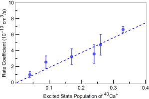
Figure 6: Charge-exchange rate coefficient as a function of the ⁴⁰Ca⁺(4P_1/2) excited-state population. The error bars are one standard deviation uncertainties based on ten measurements.

III Theoretical models for the charge-exchange reaction

III.1 Charge exchange in the presence of the Ca⁺ ion cooling laser

Our experimental measurements provide clear evidence of the important role that the excitation of ⁴⁰Ca⁺ ions into the 4p²P_1/2 state plays in changing the charge exchange rate. To better understand the reaction mechanism we theoretically studied the excited-state electronic potentials of the KCa⁺ molecule in order to identify processes that lead to high-yield reaction channels and the formation of K⁺ ions as well as neutral excited-state Ca atoms.

Enhanced collisional charge-exchange rate occurs when molecular energy levels of Ca⁺K and K⁺Ca configurations are energetically close allowing for efficient charge exchange. As shown in Fig. 7 we find such conditions in collisional interactions between ground state K(²S_1/2) atoms and electronically-excited Ca⁺(${}^{2}{\rm P}_{j=1/2}$) ions on the one hand and between ground state K⁺(¹S₀) ions and metastable Ca(3d4p ${}^{3}{\rm P}_{j=1}$) atoms on the other. These two dissociation limits are only separated by 150 cm^-1 energy equivalent and have energies lying approximately ${E/hc=25000}$ cm^-1 above the K(4s ²S_1/2) + Ca⁺(²S_1/2) ground state. This latter energy corresponds to a photon with a wavelength of 397 nm, the wavelength of the cooling laser for the Ca⁺ ion. Figure 7b) also shows that potentials dissociating to the two nearly-degenerate dissociation limits have an avoided crossing near $28a_{0}$ leading to significant charge exchange. The zero of energy in Figure 7 is at the ${\rm K}(^{2}{\rm S}_{1/2})+{\rm Ca}^{+}(^{2}{\rm S}_{1/2})$ dissociation limit.

Figure 7 is based on an implicit approximation for our coordinate system that will be used throughout this paper. In charge exchange an electron moves from one atom to another, thereby, changing the center of charge and mass of the dimer. We assume that the effects of these changes on rate coefficients is negligible and express all molecular interactions in terms of separation $\vec{R}=(R,\theta,\varphi)$ in spherical coordinates defined as the distance $R$ between and orientation $\theta,\varphi$ of the center of mass of neutral ³⁹K with respect to that of the center of mass of ionic ⁴⁰Ca⁺ in a laboratory-fixed coordinate frame. The reduced mass $\mu=m_{\rm K}m_{\rm Ca}/(m_{\rm K}+m_{\rm Ca})$ is that of the ³⁹K+⁴⁰Ca⁺ system, where $m_{\rm K}$ and $m_{\rm Ca}$ are the masses of ³⁹K and ⁴⁰Ca⁺, respectively.

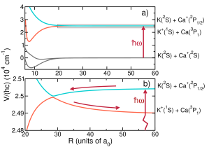
Figure 7: a) Schematic of the relevant electronic potential energy curves as functions of the K+Ca⁺ separation $R$. Only curves relevant for charge-exchange starting from the absorption of a photon from the ${\rm K}(^{2}{\rm S}_{1/2})+{\rm Ca}^{+}(^{2}{\rm S}_{1/2})$ to ${\rm K}(^{2}{\rm S}_{1/2})+{\rm Ca}^{+}(^{2}{\rm P}_{1/2})$ the channels are shown. From low to high energy the two potentials dissociating to the ${\rm K}(^{2}{\rm S}_{1/2})+{\rm Ca}^{+}(^{2}{\rm S}_{1/2})$ limit have ${}^{1}\Sigma^{+}$ and ${}^{3}\Sigma^{+}$ symmetry, respectively. The zero of energy is at the ${\rm K}(^{2}{\rm S}_{1/2})+{\rm Ca}^{+}(^{2}{\rm S}_{1/2})$ dissociation limit and $a_{0}$ is the Bohr radius. Panel b) zooms in on the potentials leading to charge exchange to ${\rm K}^{+}(^{1}{\rm S}_{1/2})+{\rm Ca}(^{3}{\rm P}_{1})$ releasing only 150 cm^-1 equivalent kinetic energy. The gray box in panel a) corresponds to the energy and separation region shown in panel b).

The reaction between atoms and ions is governed by four interactions: a) an isotropic and anisotropic $C_{4}/R^{4}$ induction interaction between the charge of an ion and the induced dipole moment of a neutral atom; b) an anisotropic $C_{3}/R^{3}$ interaction between the ion charge and the quadrupole moment of an excited neutral atom; c) the spin-orbit interaction that defines splitting of the Ca⁺(4p ${}^{2}{\rm P}_{j}$) and Ca(3d4p ${}^{3}{\rm P}_{j}$ fine-structure states; d) the molecular rotation. Both $C_{4}$ and $C_{3}$ coefficients orientationally dependent and defined byproperties of the neutral atom. Dispersive van-der-Waals potentials do not significantly contribute to the atom-ion interaction for $R>20a_{0}$.

If we ignore the rotation of the molecule for the moment, a convenient basis for the reaction from ${\rm K}({\rm 4s}\,^{2}{\rm S}_{j_{a}})+{\rm Ca}^{+}({\rm 4p}\,^{2}{\rm P}_{j_{b}})$ to ${\rm K}^{+}(^{1}{\rm S}_{j^{\prime}_{a}})+{\rm Ca}({\rm 3d4p}\,^{3}{\rm P}_{j^{\prime}_{b}})$ is the body-fixed product basis

$$|q_{a},j_{a},\Omega_{a}\rangle|q_{b},j_{b},\Omega_{b}\rangle\,,$$ (1)

where $q_{i}=0,+1$ is charge state of the atom or ion $i=a$ and $b$ for K/K⁺ and Ca/Ca⁺, respectively, and $\Omega_{i}$ is the projection quantum number of the total atomic/ionic angular momentum $\vec{\jmath}_{i}$ along the interatomic axis $\vec{R}$. We use that within the context of this charge-exchange process labels $q_{i}$, $j_{i}$, and $\Omega_{i}$ uniquely specify an atomic/ionic state. A list of states can be found in Table 1.

Table 1: The quantum numbers for our body-fixed basis states for the ${\rm K}({\rm 4s}\,^{2}{\rm S}_{j_{a}})+{\rm Ca}^{+}({\rm 4p}\,^{2}{\rm P}_{j_{b}})$ to ${\rm K}^{+}(^{1}{\rm S}_{j^{\prime}_{a}})+{\rm Ca}({\rm 3d4p}\,^{3}{\rm P}_{j^{\prime}_{b}})$ reaction and the corresponding diagonal $C_{3}$ and $C_{4}$ coefficients in atomic units. Channels are uniquely described by the charge $q_{i}$, atomic angular momenta $j_{i}$, and its body-fixed projection $\Omega_{i}$ on the internuclear axis with $i=a$ and $b$ for K and Ca, respectively. Potentials are degenerate for $-\Omega$ and $\Omega$, where $\Omega=\Omega_{a}+\Omega_{b}$.

K or K+			Ca or Ca+
$q_{a}$	$j_{a}$	$\Omega_{a}$	$q_{b}$	$j_{b}$	$\Omega_{b}$	$C_{3}$	$C_{4}$
0	$1/2$	$1/2$	+1	1/2	$-1/2$	0	$-$145.29
0	$1/2$	$-1/2$	+1	1/2	1/2	0	$-$145.29
0	1/2	1/2	+1	1/2	1/2	0	$-$145.29
+1	0	0	0	0	0	0	$-$641.0
+1	0	0	0	1	0	5.874	97.95
+1	0	0	0	1	1	$-$2.937	$-$1015.5
+1	0	0	0	2	0	$-$5.874	$-$1404.7
+1	0	0	0	2	1	$-$2.937	$-$1027.9
+1	0	0	0	2	2	5.874	102.7

The matrix elements of the two long-range molecular interactions are diagonal in and independent of the quantum numbers of the ion and only depend on the state of the neutral atom. In fact,

$$\frac{\langle 0,j_{s},\Omega_{s}|C_{3}|0,j^{\prime}_{s},\Omega^{\prime}_{s}\rangle}{R^{3}} = \delta_{\Omega_{s}\Omega^{\prime}_{s}}\frac{q}{R^{3}}(-1)^{j_{s}-\Omega_{s}}$$

$$\quad\times\begin{pmatrix}j_{s}&2&j^{\prime}_{s}\\ -\Omega_{s}&0&\Omega_{s}\end{pmatrix}\langle j_{s}||Q_{2}||j^{\prime}_{s}\rangle$$

in atomic units for the neutral atom with quantum numbers $j_{s}\Omega_{s}$ Tomza et al. (2019). Here, $q=+1$ for the corresponding ion, $\delta_{\Omega\Omega^{\prime}}$ is the Kronecker delta, and (:::) denotes a Wigner 3-$j$ symbol. The matrix elements of the induction potential for K(4s ²S) are

$$\frac{\langle 0,j_{s},\Omega_{s}|C_{4}|0,j^{\prime}_{s},\Omega^{\prime}_{s}\rangle}{R^{4}}=-\delta_{j_{s}\Omega_{s},j^{\prime}_{s}\Omega^{\prime}_{s}}\frac{q^{2}}{2R^{4}}\alpha_{0,s}\,,$$

while the diagonal matrix elements of the induction potential for Ca(3d4p ²P) states are

$$\frac{\langle 0,j_{s},\Omega_{s}|C_{4}|0,j_{s},\Omega_{s}\rangle}{R^{4}} = -\frac{q^{2}}{2R^{4}}\quad$$

$$\times \left[\alpha_{0,s}+\alpha_{2,s}\frac{3\Omega_{s}^{2}-j_{s}(j_{s}+1)}{j_{s}(2j_{s}-1)}\right]\,,$$

from Ref. Mitroy et al. (2010). Off-diagonal matrix elements, coupling states with $|\Delta j_{s}|\leq 2$, can also be found in Ref. Mitroy et al. (2010). Finally, $\langle j_{s}||Q_{2}||j_{s}\rangle$, $\alpha_{0,s}$, and $\alpha_{2,s}$ are the reduced quadrupole-moment matrix elements and static scalar and tensor polarizabilities of the neutral atom $s$ with angular momentum $j_{s}$, respectively. The sum $\Omega=\Omega_{a}+\Omega_{b}$ is conserved for both interactions.

We have calculated the reduced matrix element of the quadrupole moment of Ca(3d4p ³P) states using a non-relativistic multi-configuration-interaction method with an all-electron correlation-consistent polarized valence-only quintuple zeta (CC-pV5Z) basis set Koput and Peterson (2002). For the triplet states calculations have been performed in the $B_{3u}$ representation. More details of our calculation can be found Supplemental Material. This calculation provides the expectation value of the quadrupole operator $\hat{Q}_{20}$ for state $|0,j_{s}=1,\Omega_{s}=0\rangle$ of neutral Ca(3d4p ³P). The value is $-11.748$ a.u. with an one-standard-deviation uncertainty of 3.0 a.u. (Here, a.u. is an abbreviation for atomic unit and we keep all digits to avoid roundoff problems.) Of course, the quadrupole moment for an S state is zero.

We used the static scalar polarizability of $290.48$ a.u. for K($4{\rm s}\,^{2}{\rm S}_{1/2}$) from Ref. Holmgren et al. (2010). For Ca(3d4p ${}^{3}{\rm P}_{0,1,2}$) states we have computed $\alpha_{0,s}$ and $\alpha_{2,s}$ using transition dipole moments from Yu and Derevianko (2018) and perturbation theory. Values for quadrupole moments and static polarizabilities are summarized in Table 2. Table 1 lists the diagonal $C_{3}$ and $C_{4}$ coefficients for the relevant channels $|q_{a},j_{a}\Omega_{a}\rangle|q_{b},j_{b}\Omega_{b}\rangle$.

The charge-exchange-inducing coupling between the body-fixed channels is computed based on the application of the Heitler-London method, in which the electron in the 4s orbital of K moves to the unoccupied 3d orbital of Ca⁺. The coupling is then given by the overlap integral of these non-relativistic atomic Hartree-Fock orbitals and the electron-nucleus Coulomb interaction potential. The coupling matrix element between channels $|0,j_{a}\Omega_{a}\rangle|{+1},j_{b}\Omega_{b}\rangle$ and $|{+1},j^{\prime}_{a}\Omega^{\prime}_{a}\rangle|0,j^{\prime}_{b}\Omega^{\prime}_{b}\rangle$ with the same $\Omega=\Omega_{a}+\Omega_{b}=\Omega^{\prime}_{a}+\Omega^{\prime}_{b}$=0, 1 are $\sqrt{\frac{2}{30}}O(R)$ and $\sqrt{\frac{1}{30}}O(R)$, respectively, where

$$O(R) = \int d^{3}r\,\phi_{\rm K,4s}(\vec{r}-\vec{r}_{\rm K})\frac{e^{2}}{4\pi\epsilon_{0}}\left[\frac{1}{|\vec{r}-{\vec{r}}_{\rm K}|}+\frac{1}{|\vec{r}-{\vec{r}}_{\rm Ca}|}\right]$$ (2)

$$\quad\quad\quad\quad\times\phi_{\rm Ca,3d}(\vec{r}-\vec{r}_{\rm Ca})\,,$$

$\phi_{\rm K,4s}(\vec{r}-\vec{r}_{\rm K})$ and $\phi_{\rm Ca,3d}(\vec{r}-\vec{r}_{\rm Ca})$ are the spatial-components of the K(4s) and Ca(3d) Hartree-Fock electron orbitals, respectively, and $\vec{r}_{i}$ is the location of nucleus $i={\rm K}$ or Ca. For our choice of coordinate system $R=|\vec{r}_{\rm K}-\vec{r}_{\rm Ca}|$ to good approximation. The function $O(R)$ is $hc\times 5.6$ cm^-1 at $R=28a_{0}$ and rapidly goes to zero for $R\to\infty$.

Table 2: Atomic parameters in atomic units used to generate the interaction potentials. See text for definitions.

Term		$\alpha_{0}$		$\alpha_{2}$		$\langle j||Q_{2}||j\rangle$
K (4s)	${}^{2}{\rm S}_{1/2}$	290.	58
Ca (4s2)	${}^{1}{\rm S}_{0}$	157.	1
Ca (3d4p)	${}^{3}{\rm P}_{0}$	1282.	0
Ca (3d4p)	${}^{3}{\rm P}_{1}$	1288.	7	742.	3	$-$16.	086
Ca (3d4p)	${}^{3}{\rm P}_{2}$	1302.	0	$-$1507.	4	32.	173

Figure 8: Long-range adiabatic potential energy curves with $\Omega=0^{\pm}$, 1, and 2 as functions of the atom-ion separation $R$. Panels a) and c) have been computed without the charge-exchange-inducing coupling. Panel (b) shows avoided crossings among adiabatic potentials due to the charge-exchange-inducing coupling near $R=28a_{0}$. The zero of energy in all panels is located at the K(4s ${}^{2}{\rm S}_{1/2}$) + Ca⁺(4p ${}^{2}{\rm P}_{1/2}$) entrance channel (red arrow in panel a).

Figure 8 shows three views of the long-range adiabatic $\Omega=0^{\pm}$, 1 and 2 potentials for the excited-state charge-exchange reaction. Panels a) and c) have been found by diagonalizing the potential matrix at each $R$ in the body-fixed basis of Eq. 1 without the charge-exchange-inducing coupling, while in panel b) this coupling has been included. Consequently, curves dissociating to the K(4s ${}^{2}{\rm S}_{1/2}$) + Ca⁺(4p ${}^{2}{\rm P}$) limits in Fig. 8a) cross those dissociating to the K⁺(${}^{1}{\rm S}_{0}$) + Ca(3d4p ${}^{3}{\rm P}$) limits. These crossings become avoided crossings once charge-exchange-inducing couplings are included, as shown in Fig. 8b) around $R=28a_{0}$. The (avoided) crossings for the curves dissociating to the K(4s ${}^{2}{\rm S}_{1/2}$) + Ca⁺(4p ${}^{2}{\rm P}_{3/2}$) limits are not energetically-accessible from our K(4s ${}^{2}{\rm S}_{1/2}$) + Ca⁺(4p ${}^{2}{\rm P}_{1/2}$) entrance channels and need not be considered further. Charge exchange can only occur between states with the same $\Omega$, which in our system only occurs between $\Omega=0^{\pm}$ and 1 potentials. The asymptotic splittings between the entrance channel and the exit channels is approximately $hc\times 150$ cm^-1. The zero of energy in all panels is located at the K(4s ${}^{2}{\rm S}_{1/2}$) + Ca⁺(4p ${}^{2}{\rm P}_{1/2}$) entrance channel.

For the experimental temperature near 0.1 K and a long-range induction potential, the number of partial waves or relative orbital angular momenta of the atom-ion system, $\vec{\ell}$, contributing to the charge-exchange rate coefficient is large. Then we are justified in approximating the rotational Hamiltonian of the diatom and use the infinite-order sudden approximation Nikitin (2006). This corresponds to performing coupled-channels calculations for each triple $J$, $M$, and $\Omega$ in the channel basis $\sqrt{(2J+1)/8\pi^{2}}D^{J*}_{M\Omega}(\varphi,\theta,0))|q_{a},j_{a}\Omega_{a}\rangle|q_{b},j_{b}\Omega_{b}\rangle$ ignoring couplings between different $\Omega^{\pm}$ and using a diagonal centrifugal potential with matrix element $\hbar^{2}J(J+1)/2\mu R^{2}$ for each channel independent of $M$ and $\Omega^{\pm}$. Here, $D^{j}_{mm^{\prime}}(\alpha\beta\gamma)$ is a Wigner rotation matrix, $\Omega=\Omega_{a}+\Omega_{b}$, $\vec{J}=\vec{\jmath}_{a}+\vec{\jmath}_{b}+\vec{\ell}$ is the total molecular angular momentum with projection quantum number $M$. For $\Omega=0^{-}$, $0^{+}$, and 1 channels are coupled for each $J$ and $M$, respectively, as we can ignore the effects of the energetically-closed K(4s ${}^{2}{\rm S}_{1/2}$) + Ca⁺(4p ${}^{2}{\rm P}_{3/2}$) channels. For a valid coupled-channels calculation we extend the potentials to $R\to 0^{+}\,a_{0}$ to have a repulsive inner wall by adding repulsive $C_{12}/R^{12}$ potentials to the diagonal potential matrix elements in the channel states. Typical examples can be seen in Fig. 7.)

We propagate the wavefunctions in the coupled-channels calculations for each $J,M,\Omega^{\pm}$ using Gordon’s propagator Gordon (1969) and match to scattering boundary conditions at large $R$ to obtain partial charge-exchange rate coefficients $K_{JM,\Omega^{\pm}}(E)$, where $E$ is the entrance-channel collision energy and have summed over all exit channels.

$$K(E)=\sum_{\Omega^{p}=0^{+},0^{-},1}g_{\Omega^{p}}\sum_{J=0}^{\infty}(2J+1)K_{JM,\Omega^{p}}(E)\;,$$ (3)

where $g_{0^{+}}$=1/4, $g_{0^{-}}$= 1/4, and $g_{1}$=1/2.

Finally, we thermally average assuming a Gaussian distribution with a temperature $T_{\rm K}$ and $T_{\rm Ca}$ for ³⁹K and ⁴⁰Ca⁺, respectively. This distribution is used for the trapped ion cloud and based on the evidence that the effective trapping area is limited to a certain radius Delahaye (2019), which increases the likely-hood of low energy ions above that of a Maxwell-Boltzmann distribution. The thermalized total rate coefficient then only depends on the effective temperature

$$T_{\rm eff}=\frac{m_{\rm K}T_{\rm Ca}+m_{\rm Ca}T_{\rm K}}{M}\approx\frac{m_{\rm K}}{M}T_{\rm Ca}\,.$$

where $M=m_{\rm K}+m_{\rm Ca}$ and the second approximate equality follows from $T_{\rm K}\ll T_{\rm Ca}$ in our experiments. Figure 9 shows results for the total charge-exchange rate coefficient from our coupled-channels calculations and compares them to our measurement at $T_{\rm eff}=0.2$ K. The figure first shows a rate coefficient as a function of collision energy $E$. The rate coefficient has many peaks resulting from shape resonances contained by the barrier created by the attractive induction potential and the repulsive centrifugal potential. At $E/k<0.2$ K already twelve such resonances can be observed. Here, $k$ is the Boltzmann constant. In fact, for $E/k=0.2$ K at least forty $J$ contribute significantly to the total charge-exchange rate coefficient. Once the rate coefficient is thermally-averaged the peaks smooth out and the rate coefficient is a slowly increasing function with $T_{\rm eff}$ for $T_{\rm eff}<1$ K. Finally, we have studied the effects of changing the quadrupole moment and thus the $C_{3}$ coefficient within its 20% uncertainty on the thermalized rate coefficient. As shown in Fig. 9 we observe that the rate coefficient changes by 10% to 20% for temperatures between 0.01 K and 1 K. The theoretical rate coefficient is in agreement with the experimental value at $T_{\rm eff}=0.2$ K.

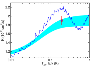
Figure 9: ${\rm K}+{\rm Ca}^{+}\to{\rm K}^{+}+{\rm Ca}$ charge-exchange rate coefficients in the presence of the Ca⁺-ion cooling laser based on coupled-channels calculations as a function of collision energy $E$ or effective temperature $T_{\rm eff}$ as defined in the text. The brown curve shows an example of rate coefficient $K(E)$ as a function of collision energy $E$. The cyan colored band corresponds to the thermally-averaged rate coefficient as a function of $T_{\rm eff}$. The width of the band reflects our estimate of the one-standard deviation uncertainty of the coupled channels calculations. Finally, the red marker with one-standard deviation error bars is our experimentally measured thermally-averaged rate coefficient at $T_{\rm eff}=0.2$ K.

III.2 Other charge-exchange pathways in the K and Ca⁺ system

In this subsection we discuss three other processes that lead to charge exchange between colliding a K atom and a Ca⁺ ion. Their rate coefficients turn out to be much smaller than that for the process described in the previous section. A priori this was not obvious. For completeness, we briefly describe our calculations of these processes. The first process (pathway I) is simply given by the non-radiative process

$${\rm K}(^{2}{\rm S}_{1/2})+{\rm Ca}^{+}(^{2}{\rm S}_{1/2})\to{\rm K}^{+}(^{1}{\rm S}_{0})+{\rm Ca}(^{1}{\rm S}_{0})\,.$$

As already schematically shown in Fig. 7a, K+Ca⁺ collide on a ${}^{1}\Sigma^{+}$ and ${}^{3}\Sigma^{+}$ potential of the KCa⁺ molecule. A second process (pathway II) is a radiative process and combines

$${\rm K}(^{2}{\rm S}_{1/2})+{\rm Ca}^{+}(^{2}{\rm S}_{1/2})\to{\rm K}^{+}(^{1}{\rm S}_{0})+{\rm Ca}(^{1}{\rm S}_{0})+\hbar\omega$$

and

$${\rm K}(^{2}{\rm S}_{1/2})+{\rm Ca}^{+}(^{2}{\rm S}_{1/2})\to{\rm KCa}^{+}({\rm X}\,^{1}\Sigma^{+})+\hbar\omega\,,$$

where the colliding atom and ion spontaneously emit photons with energy $\hbar\omega$. In the second contribution a molecular ion is formed. Finally, non-radiative pathway III is

$${\rm K}(^{2}{\rm P}_{3/2})+{\rm Ca}^{+}(^{2}{\rm S}_{1/2})\to{\rm K}^{+}(^{1}{\rm S}_{0})+{\rm Ca}(^{1}{\rm P}_{1})\,,$$

enabled by the excitation of potassium atoms to the 4p ²P_3/2 state due to the absorption of a MOT photon.

Unlike for the calculations in the previous subsection, we have calculated accurate Born-Oppenheimer potential energy curves $V_{s}(R)$ for all separations $R$. Since the structure of KCa⁺ was unknown, we calculated all ${}^{2S+1}\Lambda^{\pm}$ non-relativistic potentials dissociating to the eight energetically-lowest asymptotes of K+Ca⁺ and K⁺+Ca, using a multi-reference configuration-interaction (MRCI) method within the MOLPRO program package Werner et al. (2012). In addition, we required the non-adiabatic coupling function $Q_{s,s^{\prime}}(R)=\langle\psi_{s};R|d/dR|\psi_{s^{\prime}};R\rangle$ and electronic transition dipole moment $d_{ss^{\prime},\rm e}(R)=\langle\psi_{s};R|\hat{d}|\psi_{s^{\prime}};R\rangle$ between the two energetically-lowest ${}^{1}\Sigma^{+}$ states, where kets $|\psi_{s};R\rangle$ denote the $R$-dependent adiabatic electronic eigen states and $\hat{d}$ is the electronic dipole operator. Details of these calculations are given in Supplemental Material.

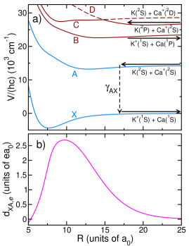
Figure 10: Panel a) The energetically-lowest five ${}^{1}\Sigma^{+}$ Born-Oppenheimer potential energy curves, labeled X, A, B, C, and D, as functions of separation $R$. The potentials have been computed with a multi-reference configuration-interaction method. The arrows indicate the entrance channels for the three pathways discussed in Sec. III.2. The blue curves are relevant for pathways I and III. Red curves are relevant for pathway II. The vertical dashed arrow labeled $\gamma_{\rm AX}$ represents spontaneous emission from state A to X in pathway III. The zero of energy is at the ${\rm K}^{+}(^{1}{\rm S}_{0})+{\rm Ca}(^{1}{\rm S}_{0})$ limit. Panel b) Electronic transition dipole moment $d_{{\rm XA},e}(R)$ between the ground X${}^{1}\Sigma^{+}$ and excited A${}^{1}\Sigma^{+}$ adiabatic Born-Oppenheimer states from our MRCI calculations. The potentials and dipole moment for $R<5a_{0}$ are not shown because the entrance channel A${}^{1}\Sigma^{+}$ potential is repulsive there and not relevant for the calculation of the rate coefficient.

Figure 10a) shows the five ${}^{1}\Sigma^{+}$ Born-Oppenheimer potentials $V_{s}(R)$ relevant for the processes described in this subsection. The long-range interaction between an atom in an S-state and an ion in an S-state is isotropic, has ${}^{1}\Sigma^{+}$ symmetry, and is described by $-C_{4}/R^{4}-C_{6}/R^{6}$. For the energetically-lowest X${}^{1}\Sigma^{+}$ state $C_{4}=78.5E_{\rm h}a_{0}^{4}$ Porsev and Derevianko (2006), while for the first-excited A${}^{1}\Sigma^{+}$ state $C_{4}=145.29E_{\rm h}a_{0}^{4}$ Holmgren et al. (2010) and $C_{6}=3866E_{\rm h}a_{0}^{6}$ Kaur et al. (2015). Here, $E_{\rm h}$ is the Hartree energy and $a_{0}$ is the Bohr radius

Non-radiative charge exchange by Pathway I

The description of cold charge-exchange collisions by pathway I involves the energetically-lowest two ${}^{1}\Sigma^{+}$ Born-Oppenheimer potentials, one ${}^{3}\Sigma^{+}$ potential, the non-adiabatic coupling between the two ${}^{1}\Sigma^{+}$ potential leading to charge exchange, but also the atomic hyperfine interaction of ${}^{39}{\rm K}(4{\rm s}\,^{2}{\rm S}_{1/2})$ between its electron and nuclear spin. The nuclear spin of ⁴⁰Ca⁺ is zero. For obtaining a qualitative estimate of rate coefficients for this pathway we can ignore the atomic hyperfine interaction Hamiltonian and then only account for the spin degeneracies.

With these approximations we can set up coupled-channels equations for charge exchange that includes only the isotropic X${}^{1}\Sigma^{+}$ and A${}^{1}\Sigma^{+}$ Born-Oppenheimer potentials, which are separated in energy by more than $hc\times 10^{3}$ cm³, using a two-channel diabatic representation that can then be used to solve the coupled-channels equations Nikitin (2006). That is, we start with the $R$-dependent electronic eigenstates $|\psi_{s};R\rangle$ with $s$=X or A for the two corresponding adiabatic Born-Oppenheimer states, respectively, and construct $R$-independent diabatic electronic basis functions $|\phi_{i}\rangle$ with $i=1,2$ based on the unitary transformation

$$\left(\begin{array}[]{c}|\phi_{1}\rangle\\ |\phi_{2}\rangle\end{array}\right)=\left(\begin{array}[]{cc}\cos\theta(R)&-\sin\theta(R)\\ \sin\theta(R)&\cos\theta(R)\end{array}\right)\left(\begin{array}[]{c}|\psi_{\rm X};R\rangle\\ |\psi_{\rm A};R\rangle\end{array}\right)$$ (4)

with mixing angle $\theta(R)=\int_{R}^{\infty}Q_{\rm X,A}(R^{\prime})dR^{\prime}$ and non-adiabatic coupling $Q_{\rm X,A}(R)$ as obtained by our MRCI calculations. The potential matrix elements $U_{ij}(R)$ in the diabatic basis $|\phi_{i}\rangle$ are then

$$U_{11}(R)=V_{\rm X}(R)\cos^{2}\theta+V_{\rm A}(R)\sin^{2}\theta\,,$$

$$U_{22}(R)=V_{\rm X}(R)\sin^{2}\theta+V_{\rm A}(R)\cos^{2}\theta\,,$$ (5)

$$U_{12}(R)=U_{21}(R)=(V_{\rm A}(R)-V_{\rm X}(R))\cos\theta\sin\theta\,.$$

Figures 10a) and 11 shows all ingredients and results of the process to create $R$-independent electronic wavefunctions. Specifically, the inputs are $V_{\rm X}(R)$ and $V_{\rm A}(R)$ in Fig. 11a) and $Q_{\rm X,A}(R)$ in Fig. 11b). The zero of energy in Figures 10a) is at the ${\rm K}^{+}(^{1}{\rm S}_{0})+{\rm Ca}(^{1}{\rm S}_{0})$ limit. The resulting mixing angle is shown in Fig. 11c). Finally, diabatic potentials $U_{ii}(R)$ and coupling $U_{12}(R)$ are shown in Fig. 11a) and d), respectively. We note that the diabatic and adiabatic potentials in Fig. 11a) have very different shapes. This difference is due to the fact that the original adiabatic potentials are energetically well separated. The diabatic coupling near the $R=9a_{0}$ crossing point is very large. Conventionally, the diabatization is only performed for the adiabatic potentials that are energetically close.

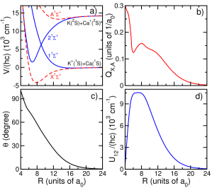
Figure 11: Diabatic representation of the ${\rm K}(^{2}{\rm S}_{1/2})+{\rm Ca}^{+}(^{2}{\rm S}_{1/2})\to{\rm K}^{+}(^{1}{\rm S}_{0})+{\rm Ca}(^{1}{\rm S}_{0})$ charge-exchange process. (a) The ground X${}^{1}\Sigma^{+}$ and excited A${}^{1}\Sigma^{+}$ adiabatic Born-Oppenheimer potentials, $V_{\rm X}(R)$ and $V_{\rm A}(R)$, (dashed red lines) and 1${}^{1}\Sigma^{+}$ and 2${}^{1}\Sigma^{+}$ diabatic potentials, $U_{11}(R)$ and $U_{22}(R)$, (solid blue lines) as functions of separation $R$. (b) the non-adiabatic coupling function $Q_{\rm X,A}(R)$ between the two ${}^{1}\Sigma^{+}$ adiabatic Born-Oppenheimer potentials as a function of $R$. Finally, panels c) and d) show mixing angle $\theta(R)$ and diabatic coupling function $U_{12}(R)$ as functions of separation $R$, respectively.

As the diabatic potential matrix elements are isotropic, we can use basis functions $|\phi_{i}\rangle Y_{\ell m}(\theta,\varphi)$ with $i$=1 and 2 to expand the total molecular wavefunction. Here, $Y_{\ell m}(\theta,\varphi)$ is a spherical harmonic, $\ell$ is the partial wave or the rotational angular momentum quantum number, and $m$ is its projection quantum number in the laboratory frame. We then solve two-channel radial coupled-channels equations for each partial wave $\ell$ and $m=0$ by numerically propagation and obtain the partial non-radiative charge-exchange (nRCE) rate coefficients $K_{\ell m}^{\rm nRCE}(E)$. The rate coefficient is the same for each $m$ and $E$ is the entrance-channel collision energy. The total rate coefficient is then

$$K_{\rm nRCE}(E)=v\sigma_{\rm nRCE}(E)=g\sum_{\ell=0}^{\infty}(2\ell+1)K_{\ell 0}^{\rm nRCE}(E)\,,$$ (6)

where $v=\sqrt{2E/\mu}$ is the relative velocity and ${g=1/4}$ is a statistical probability that accounts for the fact that the entrance threshold K$(^{2}{\rm S}_{1/2})+$Ca${}^{+}(^{2}{\rm S}_{1/2})$ has singlet and triplet total electron spin channels and that only the singlet ${}^{1}\Sigma^{+}$ channel leads to charge exchange.

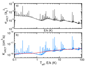
Figure 12: Panel a) Non-radiative charge-exchange cross section from K$(^{2}{\rm S}_{1/2})+$Ca${}^{+}(^{2}{\rm S}_{1/2})$ to K${}^{+}(^{1}{\rm S}_{0})+$Ca$(^{1}{\rm S}_{0})$ as a function of the entrance-channel collision energy. Panel b) Thermalized (red line) and non-thermalized rate coefficients as a function of temperature and collision energy based on the cross section shown in panel a).

Figure 12a) shows our non-radiative charge-exchange cross section $\sigma_{\rm nRCE}(E)$ for pathway I as a function of collision energies between $k\times 0.1$ K and $k\times 100$ K. The sharp resonances are again due to shape resonances of the induction potential from the forty partial waves that contribute significantly to $\sigma_{\rm nRCE}(E)$ at $E/k=0.2$ K. Thermally averaging as in Sec. III.1 assuming temperatures $T_{\rm K}$ and $T_{\rm Ca}$ for the potassium atoms and calcium ions, respectively, removes these resonances as shown in Fig. 12b). The rate coefficient is no larger than $4\times 10^{-18}$ cm³/s, eight orders of magnitude smaller than that found in Sec. III.1 and observed in our experiment.

We finish the discussion of Pathway I by artificially changing the coupling function $U_{12}(R)$ in order to better understand why our prediction for its charge-exchange rate coefficient is so small. We uniformly scale $U_{12}(R)$ and have repeated the calculation of $K_{\rm nRCE}(E)$ for various scale factors. Figure 13 shows the rate coefficient at a single collision energy as a function of $U_{12}(R)$ at $R=9a_{0}$, where the diabatic potentials cross, i.e. $U_{11}(R)=U_{22}(R)$. The figure also shows a prediction based on the Landau-Zener curve-crossing model Zhu and Nakamura (1995); Coveney et al. (1985) using the coupling strength and value and slopes of the diabatized potentials at the crossing point. Our numerical rate coefficient has a characteristic peaked behavior in good agreement with the Landau-Zener theory. It is largest for $U_{12}(9a_{0})/hc\approx 200$ cm^-1 and rapidly decreases for both smaller and larger $U_{12}(9a_{0})$. The rate coefficient based on the Landau-Zener model does not capture the oscillatory behavior of $K_{\rm nRCE}(E)$ with coupling strength as quantum interferences are not captured. Clearly, for the physical coupling strength the rate coefficient is almost negligibly small.

Figure 13: Non-radiative charge-exchange rate coefficients for K$(^{2}{\rm S}_{1/2})+$Ca${}^{+}(^{2}{\rm S}_{1/2})$ to K${}^{+}(^{1}{\rm S}_{0})+$Ca$(^{1}{\rm S}_{0})$ as functions of diabatic coupling strength $U_{12}(R)$ at $R=9a_{0}$, the separation where the two diabatic potentials cross (See Fig. 11a) and d).) The gray curve corresponds to $K_{\rm nRCE}(E)$ at $E/k=0.2$ K, while the red curve corresponds to the rate coefficient based on Landau-Zener theory. The nominal or physical coupling strength is $U_{12}(9a_{0})/hc\approx 9500$ cm^-1 and is indicated by a blue vertical line.

III.3 Radiative charge exchange by Pathway II

The description of charge-exchange by spontaneous emission from K$(^{2}{\rm S}_{1/2})+$Ca${}^{+}(^{2}{\rm S}_{1/2})$ collisions in pathway II involves the same Born-Oppenheimer potentials as in pathway I. In addition to the potentials we require the electronic transition dipole moment between the two energetically-lowest ${}^{1}\Sigma^{+}$ adiabatic states, $d_{{\rm XA},e}(R)$ as a function of $R$. Figure 10b) shows dipole moment $d_{{\rm XA},e}(R)$ determined by our MRCI calculations. The transition dipole moment is largest near $R=10a_{0}$ close to the inner turning point of the excited A${}^{1}\Sigma^{+}$ potential for our cold collision energies. It approaches zero for large separations.

We use the optical potential (OP) approach combined with the distorted-wave Born approximation for the phase shift Zygelman and Dalgarno ; Sayfutyarova et al. (2013) to calculate the total radiative charge-exchange rate coefficient $K_{\rm RCE}(E)=v\sigma_{\rm RCE}(E)$. The cross section $\sigma_{\rm RCE}(E)$ is then

$$\sigma_{\rm RCE}(E)=\frac{\pi}{k^{2}}g\sum_{\ell=0}^{\infty}(2\ell+1)\left\{1-e^{-4\eta_{\ell}(E)}\right\}\;,$$ (7)

where wavenumber $k=\sqrt{2\mu E/\hbar^{2}}$ and the dimensionless quantity.

$$\eta_{\ell}(E) = \frac{2\pi}{3}\frac{\mu}{k}\alpha^{3}\int^{\infty}_{0}\mathrm{d}R\,|F_{\rm A}^{E\ell}(R)|^{2}$$

$$\quad\quad\quad\quad\times|d_{{\rm XA},e}(R)|^{2}[V_{\rm A}(R)-V_{\rm X}(R)]^{3}\;,$$

where $\alpha\approx 1/137$ is the fine-structure constant and $F_{\rm A}^{E\ell}(R)$ is a solution of the single-channel radial Schödinger equation for the A${}^{1}\Sigma^{+}$ potential with collision energy $E$ and partial wave $\ell$. In fact, $F_{\rm A}^{E\ell}(R)\to\sqrt{2/\pi}\sin(kR+\delta_{\rm A,\ell}(k))$ for $R\to\infty$, where $\delta_{\rm A,\ell}(k)$ is the phase shift of the A${}^{1}\Sigma^{+}$ potential. In Eq. III.3 all quantities are expressed in atomic units. Finally, ${g=1/4}$ is a statistical probability that accounts for the fact that the entrance threshold has singlet and triplet total electron spin channels and that only the singlet ${}^{1}\Sigma^{+}$ channel leads to radiative transitions.

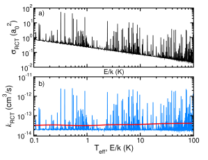
Figure 14: Panel a: Radiative charge exchange cross-section from K$(^{2}{\rm S}_{1/2})+$Ca${}^{+}(^{2}{\rm S}_{1/2})$ to K${}^{+}(^{1}{\rm S}_{0})+$Ca$(^{1}{\rm S}_{0})$ as a function of the entrance-channel collision energy. Panel b: Thermalized (ref line) and non-thermalized rate coefficients as a function of temperature and collision energy.

Figure 14a) shows our radiative charge exchange cross section $\sigma_{\rm RCE}(E)$ for pathway II as a function of collision energy. The sharp resonances are again due to shape resonances of the induction potential from the forty partial waves that contribute significantly at $E/k=0.2$ K. Thermally averaging assuming temperatures $T_{\rm K}$ and $T_{\rm Ca}$ for the potassium atoms and calcium ions, respectively, removes these resonances as shown in Fig. 14b). The rate coefficient is nearly independent of temperature and no larger than $4\times 10^{-14}$ cm³/s. This value is much larger than that for the non-radiative process in pathway I, but still four orders of magnitude smaller than observed in our experiment.

Finally, we estimate that the radiative charge-exchange rate coefficient with the reactants K$(^{2}{\rm P})$ and Ca${}^{+}(^{2}{\rm S}$) is small, of the order of 10^-14 cm³/s, based on a similar analysis as in Sec. III.C. Our experiment is not able to detect charge exchange rate coefficients of this order of magnitude.

III.4 Non-radiative charge exchange with Pathway III

A potassium atom can be resonantly excited to the 4p ²P_3/2 state by the absorption of a photon from the MOT lasers and then react with the calcium ion. That is, the reactants are ${\rm K}(^{2}{\rm P})$ and ${\rm Ca}^{+}(^{2}{\rm S})$. Unlike for Pathway I, more than one product state exists. Several of them have an electronic energy that is a few times $hc\times 10^{3}$ cm^-1 lower in energy than that of the reactants and can lead to charge exchange (See figure in Methods.) Based on the results for Pathway I and, in particular, those in Fig. 13, we limit ourselves to the product state ${\rm K}^{+}(^{1}{\rm S}_{0})+{\rm Ca}(^{1}{\rm P}_{1})$, which releases the least amount of relative kinetic energy. Even then, a model of charge exchange should include $\Sigma$ as well as $\Pi$ molecular states/channels and, as the atomic ${\rm K}(^{2}{\rm P})$ configuration is split into P_1/2 and P_3/2 states, spin-orbit interactions. As our goal is to only obtain an order of magnitude estimate for the rate coefficient it is sufficient to setup a model of charge exchange solely based on the singlet ${}^{1}\Sigma^{+}$ potentials.

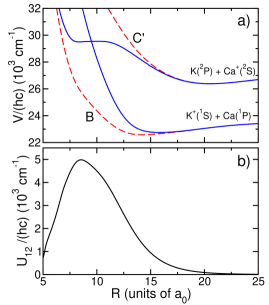
Figure 15: Potentials and couplings relevant for the non-radiative ${\rm K}(^{2}{\rm P})+{\rm Ca}^{+}(^{2}{\rm S})\to{\rm K}^{+}(^{1}{\rm S})+{\rm Ca}(^{1}{\rm P})$ charge-exchange process. (a) The excited B${}^{1}\Sigma^{+}$ Born-Oppenheimer potential and partially-diabatized C${}^{\prime}\,{}^{1}\Sigma^{+}$ potential, as defined in the text, from our MRCI calculations (dashed red lines) as functions of separation $R$. The derived diabatic potentials are shown as solid blue curves. (b) Coupling function $U_{12}(R)$ between the diabatic B and C^′ potentials as a function of $R$.

Figure 10a) shows the three relevant highly-excited ${}^{1}\Sigma^{+}$ Born-Oppenheimer potentials, each dissociating to one of the ${\rm K}^{+}(^{1}{\rm S}_{0})+{\rm Ca}(^{1}{\rm P}_{1})$, ${\rm K}(^{2}{\rm P})+{\rm Ca}^{+}(^{2}{\rm S})$, and ${\rm K}(^{2}{\rm S})+{\rm Ca}^{+}(^{2}{\rm D})$ limits. Avoided crossings between the potentials occur at multiple separations. We were, however, unable to compute the non-adiabatic coupling function $Q_{s,s^{\prime}}(R)$ among the corresponding B${}^{1}\Sigma^{+}$, C${}^{1}\Sigma^{+}$, and D${}^{1}\Sigma^{+}$ states within the MRCI method. Instead, we resort to further approximations based on the observation that the splitting between the C${}^{1}\Sigma^{+}$ and D${}^{1}\Sigma^{+}$ potentials at the avoided crossing near $R=R_{\rm CD}\equiv 15a_{0}$ is small compared to that of others at smaller separations. In fact, the splitting is much smaller than the energy difference between the C${}^{1}\Sigma^{+}$ and D${}^{1}\Sigma^{+}$ potentials at $R=R_{\rm CD}$ and that of the ${\rm K}(^{2}{\rm P})+{\rm Ca}^{+}(^{2}{\rm S})$ reactants and, classically, the crossing can not be accessed. This then implies that to good approximation we can construct a smooth diabatic potential $U_{ii}(R)$ that closely follows the D${}^{1}\Sigma^{+}$ potential for $R<R_{\rm CD}$ and the C${}^{1}\Sigma^{+}$ potential for $R>R_{\rm CD}$. We will denote this potential by C${}^{\prime}\,{}^{1}\Sigma^{+}$. The other diabatic potential will not be relevant for charge exchange as it dissociates to the ${\rm K}(^{2}{\rm S})+{\rm Ca}^{+}(^{2}{\rm D})$ limit. We omit the coupling between these two diabatic potentials.

Figure 15a) shows the B${}^{1}\Sigma^{+}$ and C${}^{\prime}\,{}^{1}\Sigma^{+}$ potentials. The potentials have a broad barely-visible avoided crossing between $7a_{0}$ and $13a_{0}$ similar in shape to that between the X${}^{1}\Sigma^{+}$ and A${}^{1}\Sigma^{+}$ potentials for Pathway I. In other words, there exist a weak non-adiabatic coupling between the adiabatic B${}^{1}\Sigma^{+}$ and C${}^{\prime}\,{}^{1}\Sigma^{+}$ states and, in fact, we will assume that the mixing angle $\theta(R)$ between states B and C^′ is the same as that between the X and A states shown in Fig. 11c). The derived diabatic potentials $U_{11}(R)$, $U_{22}(R)$, and $U_{12}(R)$ are shown in Figs. 15a) and 15b).

An further analysis of the potentials in Fig. 15 shows that the inner turning point for the reactant collision with relative kinetic energies near $E/k=1$ K is around $18a_{0}$ for both the adiabatic C${}^{\prime}\,{}^{1}\Sigma^{+}$ potential and the diabatic potential dissociating to the same limit. Moreover, the energy of the diabatic potentials at the separation where they cross is higher than that of the ${\rm K}(^{2}{\rm P})+{\rm Ca}^{+}(^{2}{\rm S})$ reactants. The crossing is not accessible when $U_{12}(R)$ is either small or large. For the physically-appropriate shape of $U_{12}(R)$, the numerically solution of the two coupled channels gives a thermalized rate coefficient of less than $10^{-18}$ cm³/s at $T_{\rm eff}=0.2$ K, smaller than that for pathway I.

IV Discussions

We have presented our experimental and theoretical investigations of charge exchange interaction between cold ⁴⁰Ca⁺ ions and ³⁹K atoms. Our theoretical analysis of all possible collision pathways confirms that the reaction occurs via the ${\rm K}(^{2}{\rm S}_{1/2})+{\rm Ca}^{+}(^{2}{\rm P}_{1/2})\rightarrow{\rm K}^{+}({\rm{}^{1}S}_{0})+Ca(3d4p^{3}{\rm P}_{1})+\hbar\omega$ channel. The experimentally measured charge exchange rate coefficient is in good agreement with our theoretical calculations.

In the future, it is possible to induce non-adiabatic transition between the first and the second electronic potentials of KCa⁺ molecules using an additional high intensity laser. One of the near future goal is to study the effect of this strong interaction on the charge exchange rate.

Over the past decade, hybrid traps proved to be a good platform to study the elastic as well as rich chemical interactions between cold atoms and ions. The next step ahead is to use this platform for attaining the ro-vibrational ground state of molecular ions. The laser cooled atomic ions can efficiently cool the translational degrees of freedom of the molecular ions Kimura et al. (2011); Rugango et al. (2015) and the internal states of the molecular ions can be sympathetically cooled using ultra cold atoms. Research towards this goal over the past few years shows promising results Rellergert et al. (2013); Hansen et al. (2014). Our next goal involves introducing CaH⁺ molecular ions to the hybrid apparatus and cooling their internal and external degrees of freedom using cold K atoms and Ca⁺ ions. However, the undesired interactions between the atoms, ions and molecular ions Hudson (2009) as well as unwanted dissociation Jyothi et al. (2016) of the molecular ions in the presence of lasers need to be controlled to achieve this goal. For instance, by manipulating the electronic state population of the ⁴⁰Ca⁺ ions we could control the K-Ca⁺ interaction rate and increase the ⁴⁰Ca⁺ ions lifetime in the presence of K atoms from 2 s to 12 s. Internal state cooling of molecular ions can be observed in the time scale of milliseconds. The already established resolved ro-vibrational spectroscopy measurement of CaH⁺ Calvin et al. can be used for the detection of the internal cooling of CaH⁺. Once prepared in the ground state, the CaH⁺ molecular ions are well suited for the test of fundamental theories such as time variation of the proton to electron mass ratio Schiller and Korobov (2005).