Generalized Parallel Tempering on Bayesian Inverse Problems

Abstract

In the current work we present two generalizations of the Parallel Tempering algorithm in the context of discrete-time Markov chain Monte Carlo methods for Bayesian inverse problems. These generalizations use state-dependent swapping rates, inspired by the so-called continuous time Infinite Swapping algorithm presented in [Plattner, Nuria, et al. 2011. J. Chem Phys. 135.13: 134111]. We analyze the reversibility and ergodicity properties of our generalized PT algorithms. Numerical results on sampling from different target distributions, show that the proposed methods significantly improve sampling efficiency over more traditional sampling algorithms such as Random Walk Metropolis, preconditioned Crank-Nicolson, and (standard) Parallel Tempering.

This article has been published as Latz, J., Madrigal-Cianci, J.P., Nobile, F. et al. Generalized parallel tempering on Bayesian inverse problems. Stat Comput 31, 67 (2021). https://doi.org/10.1007/s11222-021-10042-6, and can be accessed here: https://rdcu.be/cznfD

1 Introduction

Modern computational facilities and recent advances in computational techniques have made the use of Markov Chain Monte Carlo (MCMC) methods feasible for some large-scale Bayesian inverse problems (BIP), where the goal is to characterize the posterior distribution of a set of parameters $\theta$ of a computational model which describes some physical phenomena, conditioned on some (usually indirectly) measured data $y$. However, some computational difficulties are prone to arise when dealing with difficult to explore posteriors, i.e., posterior distributions that are multi-modal, or that concentrate around a non-linear, lower-dimensional manifold, since some of the more commonly-used Markov transition kernels in MCMC algorithms, such as random walk Metropolis (RWM) or preconditioned Crank-Nicholson (pCN), are not well-suited in such situations. This in turn can make the computational time needed to properly explore these complicated target distributions arbitrarily long. Some recent works address these issues by employing Markov transitions kernels that use geometric information beskos2017geometric ; however, this requires efficient computation of the gradient of the posterior density, which might not always be feasible, particularly when the underlying computational model is a so-called “black-box”.

In recent years, there has been an active development of computational techniques and algorithms to overcome these issues using a tempering strategy dia2019continuation ; earl2005parallel ; latz2017multilevel ; miasojedow2013adaptive ; vrugt2009accelerating . Of particular importance for the work presented here is the Parallel Tempering (PT) algorithm earl2005parallel ; lkacki2016state ; miasojedow2013adaptive (also known as replica exchange), which finds its origins in the physics and molecular dynamics community. The general idea behind such methods is to simultaneously run $K$ independent MCMC chains, where each chain is invariant with respect to a flattened (referred to as tempered) version of the posterior of interest $\mu$, while, at the same time, proposing to swap states between any two chains every so often. Such a swap is then accepted using the standard Metropolis-Hastings (MH) acceptance-rejection rule. Intuitively, chains with a larger smoothing parameter (referred to as temperature) will be able to better explore the parameter space. Thus, by proposing to exchange states between chains that target posteriors at different temperatures, it is possible for the chain of interest (i.e., the one targeting $\mu$) to mix faster, and to avoid the undesirable behavior of some MCMC samplers of getting “stuck” in a mode. Moreover, the fact that such an exchange of states is accepted with the typical MH acceptance-rejection rule, will guarantee that the chain targeting $\mu$ remains invariant with respect to such probability measure earl2005parallel .

Tempering ideas have been successfully used to sample from posterior distributions arising in different fields of science, ranging from astrophysics to machine learning desjardins2010tempered ; earl2005parallel ; miasojedow2013adaptive ; van2008parameter . The works madras2002markov ; woodard2009conditions have studied the convergence of the PT algorithm from a theoretical perspective and provided minimal conditions for its rapid mixing. Moreover, the idea of tempered distributions has not only been applied in combination with parallel chains. For example, the simulated tempering method marinari_1992 uses a single chain and varies the temperature within this chain. In addition, tempering forms the basis of efficient particle filtering methods for stationary model parameters in Sequential Monte Carlo settings Beskos16 ; Beskos15 ; kahle2018bayesian ; Kantas14 ; latz2017multilevel and Ensemble Kalman Inversion Schillings17 .

A generalization over the PT approach, originating from the molecular dynamics community, is the so-called Infinite Swapping (IS) algorithm dupuis2012infinite ; plattner2011infinite . As opposed to PT, this IS paradigm is a continuous-time Markov process and considers the limit where states between chains are swapped infinitely often. It is shown in dupuis2012infinite that such an approach can in turn be understood as a swap of dynamics, i.e., kernel and temperature (as opposed to states) between chains. We remark that once such a change in dynamics is considered, it is not possible to distinguish particles belonging to different chains. However, since the stationary distribution of each chain is known, importance sampling can be employed to compute posterior expectations with respect to the target measure of interest. Infinite Swapping has been successfully applied in the context of computational molecular dynamics and rare event simulation doll2012rare ; lu2013infinite ; plattner2011infinite ; however, to the best of our knowledge, such methods have not been implemented in the context of Bayesian inverse problems.

In light of this, the current work aims at importing such ideas to the BIP setting, by presenting them in a discrete-time Metropolis-Hastings Markov chain Monte Carlo context. We will refer to these algorithms as Generalized Parallel Tempering (GPT). We emphasize, however, that these methods are not a time discretization of the continuous-time Infinite Swapping presented in dupuis2012infinite , but, in fact, a discrete-time Markov process inspired by the ideas presented therein with suitably defined state-dependent probabilities of swapping states or dynamics. We now summarize the main contributions of this work.

We begin by presenting a generalized framework for discrete time PT in the context of MCMC for BIP, and then proceed to propose, analyze and implement two novel state-dependent PT algorithms inspired by the ideas presented in dupuis2012infinite .

Furthermore, we prove that our GPT methods have the right invariant measure, by showing reversibility of the generated Markov chains, and prove their ergodicity. Finally, we implement the proposed GPT algorithms for an array of Bayesian inverse problems, comparing their efficiency to that of an un-tempered, (single temperature), version of the underlying MCMC algorithm, and standard PT. For the base method to sample at the cold temperature level, we use Random Walk Metropolis (RWM) (Sections 5.3-5.6) or preconditioned Crank-Nicolson (Section 5.7), however, we emphasize that our methods can be used together with any other, more efficient base sampler. Experimental results show improvements in terms of computational efficiency of GPT over un-tempered RWM and standard PT, thus making the proposed methods attractive from a computational perspective. From an implementation perspective, the swapping component of our proposed methods is rejection-free, thus effectively eliminating some tuning parameters on the PT algorithm, such as swapping frequency.

We notice that a PT algorithm with state-dependent swapping probabilities has been proposed in lkacki2016state , however, such a work only consider pairwise swapping of chains and a different construction of the swapping probabilities, resulting in a less-efficient sampler, at least for the BIPs addressed in this work.

Our ergodicity result relies on an $L_{2}$ spectral gap analysis. It is known rudolf2011explicit that when a Markov chain is both reversible and has a positive $L_{2}$-spectral gap, one can in turn provide non-asymptotic error bounds on the mean square error of an ergodic estimator of the chain. Our bounds on the $L_{2}$-spectral gap, however, are far from being sharp and could possibly be improved using e.g., domain decomposition ideas as in woodard2009conditions . Such analysis is left for a future work.

The rest of this paper is organized as follows. Section 2 is devoted to the introduction of the notation, Bayesian inverse problems, and Markov chain Monte Carlo methods. In Section 3, we provide a brief review of (standard) PT (Section 3.2), and introduce the two versions of the GPT algorithm in Sections 3.3 and 3.4, respectively. In fact, we present a general framework that accommodates both the standard PT algorithms and our generalized versions. In Section 4, we recall some of the standard theory of Markov chains in Section 4.1 and state the main theoretical results of the current work (Theorems 1 and 2) in Section 4.2. The proof of these Theorems is given by a series of Propositions in Section 4.2. We present some numerical experiments in Section 5, and draw some conclusions in Section 6.

2 Problem setting

2.1 Notation

Let $(W,\left\|\cdot\right\|)$ be a separable Banach space with associated Borel $\sigma$-algebra $\mathcal{B}(W)$, and let $\nu_{W}$ be a $\sigma$-finite “reference” measure on $W$. For any measure $\mu$ on $(W,\mathcal{B}(W))$ that is absolutely continuous with respect to $\nu_{W}$ (in short $\mu\ll\nu_{W}$), we define the Radon-Nikodym derivative $\pi_{\mu}\mathrel{\mathop{\mathchar 58\relax}}=\frac{\mathrm{d}\mu}{\mathrm{d}\nu_{W}}$. We denote by $\overline{\mathcal{M}}(W)$ the set of real-valued signed measures on $(W,{\mathcal{B}(W)})$, and by $\mathcal{M}(W)\subset\overline{\mathcal{M}}(W)$ the set of probability measures on $(W,{\mathcal{B}(W)})$.

Let $W_{1},W_{2}$ be two separable Banach spaces with reference measures $\nu_{W_{1}},\nu_{W_{2}}$, and let $\mu_{1}\ll\nu_{W_{1}},\mu_{2}\ll\nu_{W_{2}}$ be two probability measures, with corresponding densities given by $\pi_{\mu_{1}},\pi_{\mu_{2}}$. The product of these two measures is defined by

$$\bm{\mu}(A) =\left(\mu_{1}\times\mu_{2}\right)(A)$$ (1)

$$=\iint_{A}\pi_{\mu_{1}}(\theta_{1})\pi_{\mu_{2}}(\theta_{2})\nu_{W_{1}}(\mathrm{d}\theta_{1})\nu_{W_{2}}(\mathrm{d}\theta_{2}),$$ (2)

for all $A\in\mathcal{B}(W_{1}\times W_{2}).$ Joint measures on $(W_{1}\times W_{2},\mathcal{B}(W_{1},\times W_{2}))$ will always be written in boldface.

A Markov kernel on a Banach space $W$ is a function $p\mathrel{\mathop{\mathchar 58\relax}}W\times\mathcal{B}(W)\rightarrow[0,1]$ such that

1. For each $A$ in $\mathcal{B}(W)$, the mapping $W\ni\theta\mapsto p(\theta,A)$, is a $\mathcal{B}(W)$-measurable real-valued function.

2. For each $\theta$ in $W$, the mapping $\mathcal{B}(W)\ni A\mapsto p(\theta,A)$, is a probability measure on $(W,\mathcal{B}(W))$.

We denote by $P$ the Markov transition operator associated to $p$, which acts on measures as $\nu\mapsto\nu P\in\mathcal{M}(W),$ and on functions as $f\mapsto Pf,$ with $Pf$ measurable on $(W,\mathcal{B}(W)),$ such that

$$(\nu P)(A) =\int_{W}p(\theta,A)\nu(\mathrm{d}\theta),\quad\forall A\in{\mathcal{B}(W)},$$ (3)

$$(Pf)(\theta) =\int_{W}f(z)p(\theta,\mathrm{d}z),\quad\forall\theta\in W.$$ (4)

Let $P_{k},\ k=1,2,$ be Markov transition operators associated to kernels $p_{k}\mathrel{\mathop{\mathchar 58\relax}}W_{k}\times\mathcal{B}(W_{k})\mapsto[0,1].$ We define the tensor product Markov operator $\mathbf{P}\mathrel{\mathop{\mathchar 58\relax}}=P_{1}\otimes P_{2}$ as the Markov operator associated with the product measure $\mathbf{p}(\bm{\theta},\cdot)=p_{1}(\theta_{1},\cdot)\times p_{2}(\theta_{2},\cdot),\ \bm{\theta}=(\theta_{1},\theta_{2})\in W_{1}\times W_{2}$. In particular, $\bm{\nu}\mathbf{P}$ is the measure on $(W_{1}\times W_{2},\mathcal{B}(W_{1}\times W_{2}))$ that satisfies

$$(\bm{\nu}\mathbf{P})(A_{1}\times A_{2}) =\iint_{W_{1}\times W_{2}}p_{1}(\theta_{1},A_{1})p_{2}(\theta_{2},A_{2})\bm{\nu}(\mathrm{d}\theta_{1},\mathrm{d}\theta_{2}),$$ (5)

for all $A_{1}\in\mathcal{B}(W_{1})$ and $A_{2}\in\mathcal{B}(W_{2})$. Moreover, $(\mathbf{P}f)\mathrel{\mathop{\mathchar 58\relax}}W_{1}\times W_{2}\rightarrow\mathbb{R}$ is the function given by

$$(\mathbf{P}f)(\bm{\theta}) =\iint_{W_{1}\times W_{2}}f(z_{1},z_{2})p_{1}(\theta_{1},\mathrm{d}z_{1})p_{2}(\theta_{2},\mathrm{d}z_{2}),$$ (6)

for an appropriate $f\mathrel{\mathop{\mathchar 58\relax}}W_{1}\times W_{2}\rightarrow\mathbb{R}$.

We say that a Markov operator $P$ (resp. $\mathbf{P}$) is invariant with respect to a measure $\nu$ (resp. $\bm{\nu}$) if $\nu P=\nu$ (resp. $\bm{\nu}\mathbf{P}=\bm{\nu}$ ). A related concept to invariance is that of reversibility; a Markov kernel $p\mathrel{\mathop{\mathchar 58\relax}}W\times{\mathcal{B}(W)}\mapsto[0,1]$ is said to be reversible (or $\nu$-reversible) with respect to a measure $\nu\in\mathcal{M}(W)$ if

$$\int_{B}p(\theta,A)\nu(\mathrm{d}\theta)=\int_{A}p(\theta,B)\nu(\mathrm{d}\theta),\quad\forall A,B\in{\mathcal{B}(W)}.$$ (7)

For two given $\nu$-invariant Markov operators $P_{1},P_{2}$, we say that $P_{1}P_{2}$ is a composition of Markov operators, not to be confused with $P_{1}\otimes P_{2}$. Furthermore, given a composition of $K$ $\nu$-invariant Markov operators $P_{c}\mathrel{\mathop{\mathchar 58\relax}}=P_{1}P_{2}\dots P_{K}$, we say that $P_{c}$ is palindromic if $P_{1}=P_{K},$ $P_{2}=P_{K-1},$ …, $P_{k}=P_{K-{k+1}},\ k=1,2\dots,K$. It is known (see, e.g., (brooks2011handbook, , Section 1.12.17)) that a palindromic, $\nu$-invariant Markov operator $P_{c}$ has an associated Markov transition kernel $p_{c}$ which is $\nu$-reversible.

2.2 Bayesian inverse problems

Let $(\Theta,\left\|\cdot\right\|_{\Theta})$ and $(Y,\left\|\cdot\right\|_{Y})$ be separable Banach spaces with associated Borel $\sigma$-algebras $\mathcal{B}(\Theta),\ \mathcal{B}(Y)$. In Bayesian Inverse Problems we aim at characterizing the probability distribution of a set of parameters $\theta\in\Theta$ conditioned on some measured data $y\in Y$, where the relation between $\theta$ and $y$ is given by:

$${y}={{\mathcal{F}}}(\theta)+{\varepsilon},\quad\varepsilon\sim\mu_{\textrm{noise}}.$$ (8)

Here $\varepsilon$ is some random noise with known distribution $\mu_{\mathrm{noise}}$ (assumed to have a density $\pi_{\textrm{noise}}$ with respect to some reference measure $\nu_{Y}$ on $Y$) and $\mathcal{F}\mathrel{\mathop{\mathchar 58\relax}}\Theta\mapsto Y$ is the so-called forward mapping operator. Such an operator can model, e.g., the numerical solution of a possibly non-linear Partial Differential Equation (PDE) which takes $\theta$ as a set of parameters. We will assume that the data $y$ is finite dimensional, i.e., $Y=\mathbb{R}^{d_{y}}$ for some $d_{y}\geq 1$, and that $\theta\sim\mu_{\mathrm{pr}}$. Furthermore, we define the potential function $\Phi(\theta;y)\mathrel{\mathop{\mathchar 58\relax}}\Theta\times Y\mapsto\mathbb{R}$ as

$$\Phi(\theta;y)=-\log\left[\pi_{\textrm{noise}}(y-\mathcal{F}(\theta))\right],$$ (9)

where the function $\Phi(\theta;y)$ is a measure of the misfit between the recorded data $y$ and the predicted value $\mathcal{F}(\theta)$, and often depends only on $\left\|y-\mathcal{F}(\theta)\right\|_{Y}$. The solution to the Bayesian inverse problem is given by (see, for example, (Latz19Onthe, , Theorem 2.5))

$${\pi(\theta)}\mathrel{\mathop{\mathchar 58\relax}}=\pi(\theta|y)=\frac{1}{Z}{e^{-\Phi(\theta;y)}}{\pi_{\mathrm{pr}}(\theta)},$$ (10)

where $\mu$ (with corresponding $\nu_{\Theta}$-density $\pi$) is referred to as the posterior measure and

$$Z\mathrel{\mathop{\mathchar 58\relax}}=\int_{\Theta}\exp(-\Phi(\theta;y))\mu_{\textrm{pr}}(\mathrm{d}\theta).$$

The Bayesian approach to the inverse problem consists of updating our knowledge concerning the parameter $\theta$, i.e., the prior, given the information that we observed in Equation (8). One way of doing so is to generate samples from the posterior measure $\mu^{y}$. A common method for performing such a task is to use, for example, the Metropolis-Hastings algorithm, as detailed in the next section. Once samples $\{\theta^{(n)}\}_{n=0}^{N}$ have been obtained, the posterior expectation $\mathbb{E}_{\mu^{y}}[\mathcal{Q}]$ of some $\mu^{y}$-integrable quantity of interest $\mathcal{Q}\mathrel{\mathop{\mathchar 58\relax}}\Theta\mapsto\mathbb{R}$ can be approximated by the following ergodic estimator

$$\mathbb{E}_{\mu^{y}}[\mathcal{Q}]\approx\widehat{\mathcal{Q}}\mathrel{\mathop{\mathchar 58\relax}}=\frac{1}{N-b}\sum_{n=b}^{N}\mathcal{Q}(\theta^{(n)}),$$ (11)

where $b<N$ is the so-called burn-in period, used to reduce the bias typically associated to MCMC algorithms.

2.3 Metropolis-Hastings and tempering

We briefly recall the Metropolis-Hastings algorithm hastings1970monte ; metropolis1953equation . Let $q_{\mathrm{prop}}\mathrel{\mathop{\mathchar 58\relax}}\Theta\times\mathcal{B}(\Theta)\mapsto[0,1]$ be an auxiliary kernel. For $n=1,2,\dots,$ a candidate state $\theta^{*}$ is sampled from $q_{\mathrm{prop}}(\theta^{n},\cdot)$, and proposed as the new state of the chain at step ${n+1}$. Such a state is then accepted (i.e., we set $\theta^{n+1}=\theta^{*})$, with probability $\alpha_{\textrm{MH}}$,

$$\alpha_{\text{MH}}(\theta^{n},\theta^{*})=\min\left\{1,\frac{\pi_{\mu}(\theta^{*})q_{\mathrm{prop}}(\theta^{*},\theta^{n})}{\pi_{\mu}(\theta^{n})q_{\mathrm{prop}}(\theta^{n},\theta^{*})}\right\},$$ (12)

otherwise the current state is retained, i.e., $\theta^{n+1}=\theta^{n}$. Notice that, with a slight abuse of notation, we are denoting kernel and density by the same symbol $q_{\mathrm{prop}}$. The Metropolis-Hastings algorithm induces the Markov transition kernel $p\mathrel{\mathop{\mathchar 58\relax}}\Theta\times\mathcal{B}(\Theta)\mapsto[0,1]$

$$p(\theta,A) =\int_{A}\alpha_{\mathrm{MH}}(\theta,\theta^{*})q_{\mathrm{prop}}(\theta,\mathrm{d\theta^{*}})$$ (13)

$$+\delta_{\theta}(A)\int_{\Theta}(1-\alpha_{\mathrm{MH}}(\theta,\theta^{*}))q_{\mathrm{prop}}(\theta,\mathrm{d\theta^{*}}),$$ (14)

for every $\theta\in\Theta$ and $A\in\mathcal{B}(\Theta)$. In most practical algorithms, the proposal state $\theta^{*}$ is sampled from a state-dependent auxiliary kernel $q_{\mathrm{prop}}(\theta^{n},\cdot)$. Such is the case for random walk Metropolis or preconditioned Crank Nicolson, where $q_{\mathrm{prop}}(\theta^{n},\cdot)=\mathcal{N}(\theta^{n},\Sigma)$ or $q_{\mathrm{prop}}(\theta^{n},\cdot)=\mathcal{N}(\sqrt{1-\rho^{2}}\theta^{n},\rho\Sigma),$ $0<\rho<1$, respectively. However, these types of localized proposals tend to present some undesirable behaviors when sampling from certain difficult measures, which are, for example, concentrated over a manifold or are multi-modal earl2005parallel . In the first case, in order to avoid a large rejection rate, the “step-size” $\left\|\Sigma^{1/2}\right\|$ of the proposal kernel must be quite small, which will in turn produce highly-correlated samples. In the second case, chains generated by these localized kernels tend to get stuck in one of the modes. In either of these cases, very long chains are required to properly explore the parameter space.

One way of overcoming such difficulties is to introduce tempering. Let $\mu_{k},\mu_{\textrm{pr}}$ be probability measures on $(\Theta,\mathcal{B}(\Theta)),$ $k=1,\dots,K,$ such that all $\mu_{k}$ are absolutely continuous with respect to $\mu_{\textrm{pr}}$, and let $\{T_{k}\}_{k=1}^{K}$ be a set of $K$ temperatures such that $1=T_{1}<T_{2}<\dots<T_{K}\leq\infty$. In a Bayesian setting, $\mu_{\textrm{pr}}$ corresponds to the prior measure and $\mu_{k},k=1,\dots,K$ correspond to posterior measures associated to different temperatures. Denoting by $\pi_{k}$ the $\mu_{\mathrm{pr}}$-density of $\mu_{k}$, we set

$$\pi_{k}(\theta) \mathrel{\mathop{\mathchar 58\relax}}=\frac{e^{-\Phi(\theta;y)/T_{k}}}{Z_{k}},\quad\theta\in\Theta,$$ (15)

where $\quad Z_{k}\mathrel{\mathop{\mathchar 58\relax}}=\int_{\Theta}e^{-\Phi(\theta;y)/T_{k}}\mu_{\textrm{pr}}(\mathrm{d}\theta),$ and with $\Phi(\theta;y)$ as the potential function defined in (9). In the case where $T_{K}=\infty$, we set $\mu_{K}=\mu_{\textrm{pr}}$. Notice that $\mu_{1}$ corresponds to the target posterior measure.

We say that for $k=2,\dots,K,$ each measure $\mu_{k}$ is a tempered version of $\mu_{1}$. In general, the ${1/T_{k}}$ term in (15) serves as a “smoothing” factor, which in turn makes $\mu_{k}$ easier to explore as $T_{k}\to\infty$. In PT MCMC algorithms, we sample from all posterior measures $\mu_{k}$ simultaneously. Here, we first use a $\mu_{k}$-reversible Markov transition kernel $p_{k}$ on each chain, and then, we propose to exchange states between chains at two consecutive temperatures, i.e., chains targeting $\mu_{k},\mu_{k+1},\ k\in\{1,\dots,K-1\}$. Such a proposed swap is then accepted or rejected with a standard Metropolis-Hastings acceptance rejection step. This procedure is presented in Algorithm 1. We remark that such an algorithm can be modified to, for example, propose to swap states every $N_{s}$ steps of the chain, or to swaps states between two chains $\mu_{i},\mu_{j}$, with $i,j$ chosen randomly and uniformly from the index set $\{1,2,\dots,K\}$. In the next section we present the generalized PT algorithms which swap states according to a random permutation of the indices drawn from a state dependent probability.

Algorithm 1 Standard PT.

function Standard PT($N,\{p_{k}\}_{k=1}^{K}$, $\{\pi_{k}\}_{k=1}^{K},\ \mu_{\textrm{pr}}$)

     Sample $\theta_{k}^{(1)}\sim\mu_{\textrm{pr}},\ k=1,\dots,K$

      # Do one step of MH on each chain

     for $n=1,2,\dots,N-1$ do

         for $k=1,\dots,K$ do

              Sample $\theta_{k}^{(n+1)}\sim p_{k}(\theta_{k}^{(n)},\cdot)$

         end for

          # Swap states

         for $k=1,2,\dots,K-1$ do

              Swap states $\theta^{(n+1)}_{k}$ and $\theta^{(n+1)}_{k+1}$ with probability

$$\alpha_{\mathrm{swap}}=\min\left\{1,\frac{\pi_{k}(\theta^{(n+1)}_{k+1})\pi_{k+1}(\theta^{(n+1)}_{k})}{\pi_{k}(\theta^{(n+1)}_{k})\pi_{k+1}(\theta^{(n+1)}_{k+1})}\right\}$$

         end for

     end for

     Output $\{\theta^{(n)}_{1}\}_{n=1}^{N}$

end function

3 Generalizing Parallel Tempering

Infinite Swapping was initially developed in the context of continuous-time MCMC algorithms, which were used for molecular dynamics simulations. In continuous-time PT, the swapping of the states is controlled by a Poisson process on the set $\{1,\ldots,K\}$. Infinite Swapping is the limiting algorithm obtained by letting the waiting times of this Poisson process go to zero. Hence, we swap the states of the chain infinitely often over a finite time interval. We refer to dupuis2012infinite for a thorough introduction and review of Infinite Swapping in continuous-time. In Section 5 of the same article, the idea to use Infinite Swapping in time-discrete Markov chains was briefly discussed. Inspired by this discussion, we present two Generalizations of the (discrete-time) Parallel Tempering strategies. To that end, we propose to either (i) swap states in the chains at every iteration of the algorithm in such a way that the swap is accepted with probability one, which we will refer to as the Unweighted Generalized Parallel Tempering (UGPT), or (ii), swap dynamics (i.e., swap kernels and temperatures between chains) at every step of the algorithm. In this case, importance sampling must also be used when computing posterior expectations since this in turn provides a Markov chain whose invariant measure is not the desired one. We refer to this approach as Weighted Generalized Parallel Tempering (WGPT). We begin by introducing a common framework to both PT and the two versions of GPT.

Let $(\Theta,\left\|\cdot\right\|_{\Theta})$ be a separable Banach space with associated Borel $\sigma$-algebra $\mathcal{B}(\Theta)$. Let us define the $K$-fold product space $\Theta^{K}\mathrel{\mathop{\mathchar 58\relax}}=\bigtimes^{K}_{k=1}\Theta$,with associated product $\sigma$-algebra $\mathcal{B}^{K}\mathrel{\mathop{\mathchar 58\relax}}=\bigotimes^{K}_{k=1}\mathcal{B}(\Theta)$, as well as the product measures on $(\Theta^{K},\mathcal{B}^{K})$

$$\bm{\mu}\mathrel{\mathop{\mathchar 58\relax}}=\bigtimes^{K}_{k=1}\mu_{k},$$ (16)

where $\mu_{k}$ $k=1,\dots,K$ are the tempered measures with temperatures $1=T_{1}<T_{2}<T_{3}<\dots<T_{K}\leq\infty$ introduced in the previous section. Similarly, we define the product prior measure $\bm{\mu}_{\mathrm{pr}}\mathrel{\mathop{\mathchar 58\relax}}=\bigtimes_{k=1}^{K}\mu_{\mathrm{pr}}.$ Notice that $\bm{\mu}$ has a density $\bm{\pi}(\bm{\theta})$ with respect to $\bm{\mu}_{\textrm{prior}}$ given by

$$\bm{\pi}(\bm{\theta})=\prod_{k=1}^{K}\pi_{k}(\theta_{k}),\quad\bm{\theta}\mathrel{\mathop{\mathchar 58\relax}}=(\theta_{1},\dots,\theta_{K})\in\Theta^{K},$$ (17)

with $\pi_{i}(\theta)$ added subscript given as in (15). The idea behind the tempering methods presented herein is to sample from $\bm{\mu}$ (as opposed to solely sampling from $\mu_{1}$) by creating a Markov chain obtained from the successive application of two $\bm{\mu}$-invariant Markov kernels $\mathbf{p}$ and $\mathbf{q}$, to some initial distribution $\bm{\nu}$, usually chosen to be the prior $\bm{\mu}_{\mathrm{pr}}$. Each kernel acts as follows. Given the current state $\bm{\theta}^{n}=(\theta^{n}_{1},\dots,\theta^{n}_{K}),$ the kernel $\mathbf{p}$, which we will call the standard MCMC kernel, proposes a new, intermediate state $\tilde{\bm{\theta}}^{n+1}=(\tilde{\theta}^{n+1}_{1},\dots,\tilde{\theta}^{n+1}_{K}),$ possibly following the Metropolis-Hastings algorithm (or any other algorithm that generates a $\bm{\mu}$-invariant Markov operator). The Markov kernel $\mathbf{p}$ is a product kernel, meaning that each component $\tilde{\theta}_{k}^{n}$, $k=1\dots,K,$ is generated independently of the others. Then, the swapping kernel $\mathbf{q}$ proposes a new state $\bm{\theta}^{n+1}=(\theta_{1}^{n+1},\dots,\theta_{K}^{n+1})$ by introducing an “interaction” between the components of $\tilde{\bm{\theta}}^{(n+1)}.$ This interaction step can be achieved, e.g., in the case of PT, by proposing to swap two components at two consecutive temperatures, i.e., components $k$ and $k+1$, and accepting this swap with a certain probability given by the usual Metropolis-Hastings acceptance-rejection rule. In general, the swapping kernel is applied every $N_{s}$ steps of the chain, for some $N_{s}\geq 1$. We will devote the following subsection to the construction of the swapping kernel $\mathbf{q}$.

3.1 The swapping kernel $\mathbf{q}$

Define $\mathscr{S}_{K}$ as the collection of all the bijective maps from $\{1,2,\dots,K\}$ to itself, i.e., the set of all $K!$ possible permutations of $\mathrm{id}\mathrel{\mathop{\mathchar 58\relax}}=\{1,\dots,K\}$. Let $\sigma\in\mathscr{S}_{K}$ be a permutation, and define the swapped state $\bm{\theta}_{\sigma}\mathrel{\mathop{\mathchar 58\relax}}=(\theta_{\sigma(1)},\dots,\theta_{\sigma(K)}),$ and the inverse permutation $\sigma^{-1}\in\mathscr{S}_{K}$ such that $\sigma\circ\sigma^{-1}=\sigma^{-1}\circ\sigma=\mathrm{id}$. In addition, let $S_{K}\subseteq\mathscr{S}_{K}$ be any subset of $\mathscr{S}_{K}$ closed with respect to inversion, i.e., $\sigma\in S_{K}\implies\sigma^{-1}\in S_{K}$. We denote the cardinality of $S_{K}$ by $|S_{K}|.$

Example 1

As a simple example, consider a Standard PT as in Algorithm 1 with $K=4$. In this case, we attempt to swap two contiguous temperatures $T_{i}$ and $T_{i+1},\ i=1,2,3$. Thus, $S_{K}$ is the set of permutations $\{\sigma_{1,2},\sigma_{2,3},\sigma_{3,4}\}$ with:

$$\sigma_{1,2} =(2,1,3,4),$$ (18)

$$\sigma_{2,3} =(1,3,2,4),$$ (19)

$$\sigma_{3,4} =(1,2,4,3).$$ (20)

Notice that each permutation is its own inverse; for example:

$$\sigma_{1,2}(\sigma_{1,2})=\sigma_{1,2}((2,1,3,4))=(1,2,3,4)=\mathrm{id}.$$

To define the swapping kernel $\mathbf{q}$, we first need to define the swapping ratio and swapping acceptance probability.

Definition 1 (Swapping ratio)

We say that a function $r\mathrel{\mathop{\mathchar 58\relax}}\Theta^{K}\times S_{K}\mapsto[0,1]$ is a swapping ratio if it satisfies the following two conditions:

1. $\forall\bm{\theta}\in\Theta^{K}$, $r(\bm{\theta},\cdot)$ is a probability mass function on $S_{K}$.

2. $\forall\sigma\in S_{K}$, $r(\cdot,\sigma)$ is measurable on $(\Theta^{K},\mathcal{B}^{K})$.

Definition 2 (Swapping acceptance probability)

Let $\bm{\theta}\in\Theta^{K}$ and $\sigma,\ \sigma^{-1}\in S_{K}$. We call swapping acceptance probability the function $\alpha_{\mathrm{{swap}}}\mathrel{\mathop{\mathchar 58\relax}}\Theta^{K}\times S_{K}\mapsto[0,1]$ defined as

$$\alpha_{\mathrm{{swap}}}(\bm{\theta},\sigma)=\begin{cases}\min\left\{1,\frac{\bm{\pi}(\bm{\theta}_{\sigma})r(\bm{\theta}_{\sigma},\sigma^{-1})}{\bm{\pi}(\bm{\theta})r(\bm{\theta},\sigma)}\right\},&\text{if }r(\bm{\theta},\sigma)>0,\\ 0&\text{if }r(\bm{\theta},\sigma)=0.\end{cases}$$ (21)

We can now define the swapping kernel $\mathbf{q}$.

Definition 3 (Swapping kernel)

Given a swapping ratio $r\mathrel{\mathop{\mathchar 58\relax}}\Theta^{K}\times S_{K}\mapsto[0,1]$ and its associated swapping acceptance probability $\alpha_{\mathrm{swap}}\mathrel{\mathop{\mathchar 58\relax}}\Theta^{K}\times S_{K}\mapsto[0,1]$, we define the swapping Markov kernel $\mathbf{q}\mathrel{\mathop{\mathchar 58\relax}}\Theta^{K}\times\mathcal{B}^{K}\mapsto[0,1]$ as

$$\mathbf{q}(\bm{\theta},B)=\sum_{\sigma\in S_{K}}r(\bm{\theta},\sigma)\left[(1-\alpha_{\mathrm{{swap}}}(\bm{\theta},\sigma))\delta_{\bm{\theta}}(B)\right.$$ (22)

$$\left.+\alpha_{\mathrm{{swap}}}(\bm{\theta},\sigma)\delta_{\bm{\theta}_{\sigma}}(B)\right],\qquad\bm{\theta}\in\Theta^{K},\ B\in\mathcal{B}^{K},$$ (23)

where $\delta_{\bm{\theta}}(B)$ denotes the Dirac measure in $\bm{\theta}$, i.e., $\delta_{\bm{\theta}}(B)=1$ if $\bm{\theta}\in B$ and 0 otherwise.

The swapping mechanism should be understood in the following way: given a current state of the chain $\bm{\theta}\in\Theta^{K},$ the swapping kernel samples a permutation $\sigma$ from $S_{K}$ with probability $r(\bm{\theta},\sigma)$ and generates $\bm{\theta}_{\sigma}.$ This permuted state is then accepted as the new state of the chain with probability $\alpha_{\mathrm{swap}}(\bm{\theta},\sigma)$. Notice that the swapping kernel follows a Metropolis-Hastings-like procedure with “proposal” distribution $r(\bm{\theta},\sigma)$ and acceptance probability $\alpha_{\mathrm{swap}}(\bm{\theta},\sigma)$. Moreover, as detailed in the next proposition, such a kernel is reversible with respect to $\bm{\mu}$, since it is a Metropolis-Hastings type kernel.

Proposition 1

The Markov kernel $\mathbf{q}$ defined in (22) is reversible with respect to the product measure $\bm{\mu}$ defined in (16).

Proof

Let $A,B\in\mathcal{B}^{K}$. We want to show that

$$\int_{A}q(\bm{\theta},B)\bm{\mu}(\mathrm{d}\bm{\theta})=\int_{B}q(\bm{\theta},A)\bm{\mu}(\mathrm{d}\bm{\theta}).$$

Thus,

$$\int_{A}q(\bm{\theta},B)\bm{\mu}(\mathrm{d}\bm{\theta})=\underbrace{\sum_{\sigma\in S_{K}}\int_{A}r(\bm{\theta},\sigma)\alpha_{\textrm{swap}}(\bm{\theta},\sigma)\delta_{\bm{\theta}_{\sigma}}(B)\bm{\pi}(\bm{\theta})\bm{\mu}_{\mathrm{pr}}(\mathrm{d}\bm{\theta})}_{I}$$ (24)

$$+\underbrace{\sum_{\sigma\in S_{K}}\int_{A}r(\bm{\theta},\sigma)\left(1-\alpha_{\textrm{swap}}(\bm{\theta},\sigma)\right)\delta_{\bm{\theta}}(B)\bm{\pi}(\bm{\theta})\bm{\mu}_{\mathrm{pr}}(\mathrm{d}\bm{\theta})}_{II}.$$ (25)

Let $A_{\sigma}\mathrel{\mathop{\mathchar 58\relax}}=\{\bm{z}\in\Theta^{K}\mathrel{\mathop{\mathchar 58\relax}}\bm{z}_{\sigma^{-1}}\in A\}$, and, for notational simplicity, write $\min\{a,b\}=\{a\wedge b\},\ a,b\in\mathbb{R}$. From $I$, we have:

$$I=\sum_{\sigma\in S_{K}}\int_{A}\left\{1\wedge\frac{\bm{\pi}(\bm{\theta}_{\sigma})r(\bm{\theta}_{\sigma},\sigma^{-1})}{\bm{\pi}(\bm{\theta})r(\bm{\theta},\sigma)}\right\}r(\bm{\theta},\sigma)\bm{\pi}(\bm{\theta})\delta_{\bm{\theta}_{\sigma}}(B)\bm{\mu}_{\mathrm{pr}}(\mathrm{d}\bm{\theta})$$ (26)

$$=\sum_{\sigma\in S_{K}}\int_{A}\left\{1\wedge\frac{\bm{\pi}(\bm{\theta})r(\bm{\theta},\sigma)}{\bm{\pi}(\bm{\theta}_{\sigma})r(\bm{\theta}_{\sigma},\sigma^{-1})}\right\}r(\bm{\theta}_{\sigma},\sigma^{-1})\bm{\pi}(\bm{\theta}_{\sigma})\delta_{\bm{\theta}_{\sigma}}(B)\bm{\mu}_{\mathrm{pr}}(\mathrm{d}\bm{\theta}).$$ (27)

Then, noticing that $\bm{\mu}_{\mathrm{pr}}$ is permutation invariant, we get

$$I=\sum_{\sigma\in S_{K}}\int_{A_{\sigma}}\left\{1\wedge\frac{\bm{\pi}(\bm{\theta}_{\sigma^{-1}})r(\bm{\theta}_{\sigma^{-1}},\sigma)}{\bm{\pi}(\bm{\theta})r(\bm{\theta},\sigma^{-1})}\right\}$$ (28)

$$\qquad\qquad\times r(\bm{\theta},\sigma^{-1})\bm{\pi}(\bm{\theta})\delta_{\bm{\theta}}(B)\bm{\mu}_{\mathrm{pr}}(\mathrm{d}\bm{\theta})$$ (29)

$$=\sum_{\sigma\in S_{K}}\int_{A_{\sigma}\cap B}\left\{1\wedge\frac{\bm{\pi}(\bm{\theta}_{\sigma^{-1}})r(\bm{\theta}_{\sigma^{-1}},\sigma)}{\bm{\pi}(\bm{\theta})r(\bm{\theta},\sigma^{-1})}\right\}$$ (30)

$$\qquad\qquad\times r(\bm{\theta},\sigma^{-1})\bm{\pi}(\bm{\theta})\delta_{\bm{\theta}}(B)\bm{\mu}_{\mathrm{pr}}(\mathrm{d}\bm{\theta})$$ (31)

$$=\sum_{\sigma\in S_{K}}\int_{B}\left\{1\wedge\frac{\bm{\pi}(\bm{\theta}_{\sigma^{-1}})r(\bm{\theta}_{\sigma^{-1}},\sigma)}{\bm{\pi}(\bm{\theta})r(\bm{\theta},\sigma^{-1})}\right\}$$ (32)

$$\qquad\qquad\times r(\bm{\theta},\sigma^{-1})\bm{\pi}(\bm{\theta})\delta_{\bm{\theta}}(A_{\sigma})\bm{\mu}_{\mathrm{pr}}(\mathrm{d}\bm{\theta})$$ (33)

$$=\sum_{\sigma\in S_{K}}\int_{B}\left\{1\wedge\frac{\bm{\pi}(\bm{\theta}_{\sigma^{-1}})r(\bm{\theta}_{\sigma^{-1}},\sigma)}{\bm{\pi}(\bm{\theta})r(\bm{\theta},\sigma^{-1})}\right\}$$ (34)

$$\qquad\qquad\times r(\bm{\theta},\sigma^{-1})\bm{\pi}(\bm{\theta})\delta_{\bm{\theta}_{\sigma^{-1}}}(A)\bm{\mu}_{\mathrm{pr}}(\mathrm{d}\bm{\theta})$$ (35)

$$=\sum_{\sigma\in S_{K}}\int_{B}r(\bm{\theta},\sigma^{-1})\bm{\pi}(\bm{\theta})\alpha_{\textrm{swap}}(\bm{\theta},\sigma^{-1})\delta_{\bm{\theta}_{\sigma^{-1}}}(A)\bm{\mu}_{\mathrm{pr}}(\mathrm{d}\bm{\theta})$$ (36)

$$=\sum_{\sigma\in S_{K}}\int_{B}r(\bm{\theta},\sigma)\bm{\pi}(\bm{\theta})\alpha_{\mathrm{swap}}(\bm{\theta},\sigma)\delta_{\bm{\theta}_{\sigma}}(A)\bm{\mu}_{\mathrm{pr}}(\mathrm{d}\bm{\theta}).$$ (37)

For the second term $II$ we simply have

$$II=\sum_{\sigma\in S_{K}}\int_{A}r(\bm{\theta},\sigma)(1-\alpha_{\mathrm{swap}}(\bm{\theta},\sigma))\delta_{\bm{\theta}}(B)\bm{\pi}(\bm{\theta})\bm{\mu}_{\mathrm{pr}}(\mathrm{d}\bm{\theta})$$ (38)

$$=\sum_{\sigma\in S_{K}}\int_{A\cap B}r(\bm{\theta},\sigma)(1-\alpha_{\mathrm{swap}}(\bm{\theta},\sigma))\delta_{\bm{\theta}}(B)\bm{\pi}(\bm{\theta})\bm{\mu}_{\mathrm{pr}}(\mathrm{d}\bm{\theta})$$ (39)

$$=\sum_{\sigma\in S_{K}}\int_{B}r(\bm{\theta},\sigma)(1-\alpha_{\mathrm{swap}}(\bm{\theta},\sigma))\delta_{\bm{\theta}}(A)\bm{\pi}(\bm{\theta})\bm{\mu}_{\mathrm{pr}}(\mathrm{d}\bm{\theta}).$$ (40)

This generic form of the swapping kernel provides the foundation for both PT and GPT. We describe these algorithms in the following subsections.

3.2 The Parallel Tempering case

We first show how a PT algorithm that only swaps states between the $i^{\mathrm{th}}$ and $j^{\mathrm{th}}$ components of the chain can be cast in the general framework presented above. To that end, let $\sigma_{i,j}$ be the permutation of $(1,2,\dots,K),$ which only permutes the $i^{\mathrm{th}}$ and $j^{\mathrm{th}}$ components, while leaving the other components invariant (i.e., such that $\sigma(i)=j$, $\sigma(j)=i,$ and $\sigma(k)=k$, $k\neq i,k\neq j$). We can take $S_{K}=\{\sigma_{i,j},\ i,j=1,\dots,K\}$ and define the PT swapping ratio between components $i$ and $j$ by $r_{i,j}^{\mathrm{(PT)}}\mathrel{\mathop{\mathchar 58\relax}}\Theta^{K}\times S_{K}\mapsto[0,1]$ as

$$r_{i,j}^{\mathrm{(PT)}}(\bm{\theta},\sigma)\mathrel{\mathop{\mathchar 58\relax}}=\begin{cases}1&\text{ if }\sigma=\sigma_{i,j},\\ 0&\text{ otherwise}.\end{cases}$$ (41)

Notice that this implies that $r_{i,j}^{\mathrm{(PT)}}(\bm{\theta}_{\sigma},\sigma^{-1})=r_{i,j}^{\mathrm{(PT)}}(\bm{\theta},\sigma)$ since $\sigma^{-1}_{i,j}=\sigma_{i,j}$ and $r_{i,j}^{\mathrm{(PT)}}$ does not depend on $\bm{\theta}$, which in turn leads to the swapping acceptance probability $\alpha_{\mathrm{swap}}^{\mathrm{(PT)}}\mathrel{\mathop{\mathchar 58\relax}}\Theta^{K}\times S_{K}\mapsto[0,1]$ defined as:

$$\alpha_{\mathrm{swap}}^{\mathrm{{(PT)}}}(\bm{\theta},\sigma_{i,j}) \mathrel{\mathop{\mathchar 58\relax}}=\min\left\{1,\frac{\bm{\pi}(\bm{\theta}_{\sigma_{i,j}})}{\bm{\pi}(\bm{\theta})}\right\},$$ (42)

$$\alpha_{\mathrm{swap}}^{\mathrm{(PT)}}(\bm{\theta},\sigma) =0,\ \sigma\neq\sigma_{i,j}.$$ (43)

Thus, we can define the swapping kernel for the Parallel Tempering algorithm that swaps components $i$ and $j$ as follows:

Definition 4 (Pairwise Parallel Tempering swapping kernel)

Let $\bm{\theta}\in\Theta^{K}$, $\sigma_{i,j}\in S_{K}$. We define the Parallel Tempering swapping kernel, which proposes to swap states between the $i^{\mathrm{th}}$ and $j^{\mathrm{th}}$ chains as $\mathbf{q}_{i,j}^{\mathrm{{(PT)}}}\mathrel{\mathop{\mathchar 58\relax}}\Theta^{K}\times\mathcal{B}^{K}\mapsto[0,1]$ given by

$$\mathbf{q}_{i,j}^{\mathrm{{(PT)}}}(\bm{\theta},B)=\sum_{\sigma\in S_{K}}r_{i,j}^{\mathrm{{(PT)}}}(\bm{\theta},\sigma)\left((1-\alpha_{\mathrm{{swap}}}^{\mathrm{{{(PT)}}}}(\bm{\theta},\sigma))\delta_{\bm{\theta}}(B)\right.$$ (44)

$$\left.+\alpha_{\mathrm{{swap}}}^{\mathrm{{{(PT)}}}}(\bm{\theta},\sigma)\delta_{\bm{\theta}_{\sigma}}(B)\right)$$ (45)

$$=\left(1-\min\left\{1,\frac{\bm{\pi}(\bm{\theta}_{\sigma_{i,j}})}{\bm{\pi}(\bm{\theta})}\right\}\delta_{\bm{\theta}}(B)\right)$$ (46)

$$+\min\left\{1,\frac{\bm{\pi}(\bm{\theta}_{\sigma_{i,j}})}{\bm{\pi}(\bm{\theta})}\right\}\delta_{\bm{\theta}_{\sigma_{i,j}}}(B),\quad\forall B\in\mathcal{B}^{K}.$$ (47)

In practice, however, the PT algorithm considers various sequential swaps between chains, which can be understood by applying the composition of kernels $\mathbf{q}^{\mathrm{(PT)}}_{i,j}\mathbf{q}^{\mathrm{(PT)}}_{k,\ell}\dots$ at every swapping step. In its most common form brooks2011handbook ; earl2005parallel ; miasojedow2013adaptive , the PT algorithm, hereafter referred to as standard PT (which on a slight abuse of notation we will denote by PT), proposes to swap states between chains at two consecutive temperatures. Its swapping kernel $\mathbf{q}^{\mathrm{(PT)}}\mathrel{\mathop{\mathchar 58\relax}}\Theta^{K}\times\mathcal{B}^{K}\mapsto[0,1]$ is given by

$$\mathbf{q}^{\mathrm{(PT)}}\mathrel{\mathop{\mathchar 58\relax}}=\mathbf{q}^{\mathrm{(PT)}}_{1,2}\mathbf{q}^{\mathrm{(PT)}}_{2,3}...\mathbf{q}^{\mathrm{(PT)}}_{K-1,K}.$$ (48)

Moreover, the algorithm described in earl2005parallel , proposes to swap states every $N_{s}\geq 1$ steps of MCMC. The complete kernel for the PT kernel is then given by brooks2011handbook ; earl2005parallel ; miasojedow2013adaptive

$$\mathbf{p}^{\mathrm{(PT)}}\mathrel{\mathop{\mathchar 58\relax}}=\mathbf{q}^{\mathrm{(PT)}}_{1,2}\mathbf{q}^{\mathrm{(PT)}}_{2,3}...\mathbf{q}^{\mathrm{(PT)}}_{K-1,K}\mathbf{p}^{N_{s}},$$ (49)

where $\mathbf{p}$ is a standard reversible Markov transition kernel used to evolve the individual chains independently.

Remark 1

Although the kernel $\mathbf{p}$ as well as each of the $\mathbf{q}_{i,i+1}$ are $\bm{\mu}$-reversible, notice that (49) does not have a palindromic structure, and as such it is not necessarily $\bm{\mu}$-reversible. One way of making the PT algorithm reversible with respect to $\bm{\mu}$ is to consider the palindromic form

$$\mathbf{p}^{\mathrm{(RPT)}}\mathrel{\mathop{\mathchar 58\relax}}=$$ (50)

$$\left(\mathbf{q}^{\mathrm{(PT)}}_{1,2}\mathbf{q}^{\mathrm{(PT)}}_{2,3}...\mathbf{q}^{\mathrm{(PT)}}_{K-1,K}\right)\mathbf{p}^{N_{s}}\left(\mathbf{q}^{\mathrm{(PT)}}_{K,K-1}...\mathbf{q}^{\mathrm{(PT)}}_{3,2}\mathbf{q}^{\mathrm{(PT)}}_{2,1}\right),$$ (51)

where RPT stands for Reversible Parallel Tempering. In practice, there is not much difference between $\mathbf{p}^{\mathrm{(RPT)}}$ and $\mathbf{p}^{\mathrm{(PT)}}$, however, under the additional assumption of geometric ergodicity of the chain (c.f Section 4) having a reversible kernel is useful to compute explicit error bounds on the non-asymptotic mean square error of an ergodic estimator rudolf2011explicit .

3.3 Unweighted Generalized Parallel Tempering

The idea behind the Unweighted Generalized Parallel Tempering algorithm is to generalize PT so that (i) $N_{s}=1$ provides a proper mixing of the chains, (ii) the algorithm is reversible with respect to $\bm{\mu}$, and (iii) the algorithm considers arbitrary sets $S_{K}$ of swaps (always closed w.r.t inversion), instead of only pairwise swaps. We begin by constructing a kernel of the form (22). Let $r^{\mathrm{{(UW)}}}\mathrel{\mathop{\mathchar 58\relax}}\Theta^{K}\times S_{K}\mapsto[0,1]$ be a function defined as

$$r^{\mathrm{{(UW)}}}(\bm{\theta},\sigma)\mathrel{\mathop{\mathchar 58\relax}}=\frac{\bm{\pi}(\bm{\theta}_{\sigma})}{\sum_{\sigma^{\prime}\in S_{K}}\bm{\pi}(\bm{\theta}_{\sigma^{\prime}})},\quad\bm{\theta}\in\Theta^{K},\sigma\in S_{K}.$$ (52)

Clearly, (52) is a swapping ratio according to Definition 1. As such, given some state $\bm{\theta}\in\Theta^{K}$, $r^{\mathrm{{(UW)}}}(\bm{\theta},\sigma)$ assigns a state-dependent probability to each of the ${|S_{K}|}$ possible permutations in $S_{K}$. A permutation $\sigma\in S_{K}$ is then accepted with probability $\alpha_{\mathrm{swap}}^{\mathrm{{(UW)}}}(\bm{\theta},\sigma)$, given by

$$\alpha_{\mathrm{swap}}^{\mathrm{{(UW)}}}(\bm{\theta},\sigma)\mathrel{\mathop{\mathchar 58\relax}}=\min\left\{1,\frac{\bm{\pi}(\bm{\theta}_{\sigma})r^{\mathrm{{(UW)}}}(\bm{\theta}_{\sigma},\sigma^{-1})}{\bm{\pi}(\bm{\theta})r^{\mathrm{{(UW)}}}(\bm{\theta},\sigma)}\right\}.$$ (53)

Thus, we can define the swapping kernel for the UGPT algorithm, which takes the form of (22), with the particular choice of $r(\bm{\theta},\sigma)=r^{\mathrm{{(UW)}}}(\bm{\theta},\sigma)$ and

$$\alpha_{\mathrm{swap}}(\bm{\theta},\sigma)=\alpha_{\mathrm{swap}}^{\mathrm{{(UW)}}}(\bm{\theta},\sigma).$$

Notice that $\alpha^{\mathrm{{(UW)}}}_{\text{swap}}(\bm{\theta},\sigma)=1,\forall\sigma\in S_{K}$. Indeed, if we further examine Equation (53), we see that

$$\frac{\bm{\pi}(\bm{\theta}_{\sigma})r^{\mathrm{{(UW)}}}(\bm{\theta}_{\sigma},\sigma^{-1})}{\bm{\pi}(\bm{\theta})r^{\mathrm{{(UW)}}}(\bm{\theta},\sigma)} =\frac{\bm{\pi}(\bm{\theta}_{\sigma})}{\bm{\pi}(\bm{\theta})}\cdot\frac{\bm{\pi}(\bm{\theta})}{\bm{\pi}(\bm{\theta}_{\sigma})}\cdot\frac{\sum_{\sigma^{\prime}}\bm{\pi}(\bm{\theta}_{\sigma^{\prime}})}{\sum_{\hat{\sigma}}\bm{\pi}(\bm{\theta}_{\hat{\sigma}})}$$ (54)

$$=\frac{\bm{\pi}(\bm{\theta}_{\sigma})}{\bm{\pi}(\bm{\theta})}\cdot\frac{\bm{\pi}(\bm{\theta})}{\bm{\pi}(\bm{\theta}_{\sigma})}=1.$$ (55)

In practice, this means that the proposed permuted state is always accepted with probability 1. The expression of the UGPT kernel then simplifies as follows.

Definition 5 (unweighted swapping kernel)

The unweighted swapping kernel $\mathbf{q}^{\mathrm{{(UW)}}}\mathrel{\mathop{\mathchar 58\relax}}\Theta^{K}\times\mathcal{B}^{K}\mapsto[0,1]$ is defined as

$$\mathbf{q}^{\mathrm{{(UW)}}}(\bm{\theta},B)=\sum_{\sigma\in S_{K}}r^{\mathrm{{(UW)}}}(\bm{\theta},\sigma)\delta_{\bm{\theta}_{\sigma}}(B),\$$ (56)

$\forall\bm{\theta}\in\Theta^{K},\ B\in\mathcal{B}^{K}.$ Applying this swapping kernel successively with the kernel $\mathbf{p}=p_{1}\times p_{2}\times\dots p_{K}$ in the order $\mathbf{q}^{\mathrm{{(UW)}}}\mathbf{p}\mathbf{q}^{\mathrm{{(UW)}}}=\mathrel{\mathop{\mathchar 58\relax}}\mathbf{p}^{\mathrm{{(UW)}}}$ gives what we call Unweighted Generalized Parallel Tempering kernel $\mathbf{p}^{\mathrm{{(UW)}}}$. Lastly, we write the UGPT in operator form as

$$\mathbf{P}^{\mathrm{{(UW)}}}\mathrel{\mathop{\mathchar 58\relax}}=\mathbf{Q}^{\mathrm{{(UW)}}}\mathbf{P}\mathbf{Q}^{\mathrm{{(UW)}}},$$ (57)

where $\mathbf{P}$ and $\mathbf{Q}^{\mathrm{{(UW)}}}$ are the Markov operators corresponding to the kernels $\mathbf{p}$ and $\mathbf{q}^{\mathrm{{(UW)}}}$, respectively. We now investigate the reversibility of the UGPT kernel. We start with a rather straightforward result.

Proposition 2

Suppose that, for any $k=1,2,\dots,K,$ $p_{k}$ is $\mu_{k}$-reversible. Then, $\mathbf{p}=p_{1}\times\dots\times p_{K}$ is reversible with respect to $\bm{\mu}$.

Proof

We prove reversibility by confirming that equation (7) holds true. To that end, let $\bm{\theta}\in\Theta^{K},\ A,B\in\mathcal{B}^{K}$, where $A$ and $B$ tensorize, i.e., $A\mathrel{\mathop{\mathchar 58\relax}}=\prod_{k=1}^{K}A_{k}$ and $B\mathrel{\mathop{\mathchar 58\relax}}=\prod_{k=1}^{K}B_{k}$, with $A_{1},\ldots,A_{K},B_{1},\ldots,B_{K}\in\mathcal{B}(\Theta)$. Then,

$$\int_{A}\bm{\pi}(\bm{\theta})\mathbf{p}(\bm{\theta},B)\mathrm{d}\bm{\theta} =\prod_{k=1}^{K}\int_{A_{k}}\pi(\theta_{k})p(\theta_{k},B_{k})\mathrm{d}\theta_{k}$$ (58)

$$=\prod_{k=1}^{K}\int_{B_{k}}\pi(\theta_{k})p(\theta_{k},A_{k})\mathrm{d}\theta_{k}$$ (59)

$$=\int_{B}\bm{\pi}(\bm{\theta})\mathbf{p}(\bm{\theta},A)\mathrm{d}\bm{\theta}.$$ (60)

Showing that the previous equality holds for sets $A,B$ that tensorize is indeed sufficient to show that the claim holds for any $A,B\in\mathcal{B}^{K}$. This follows from Carathéodory’s Extension Theorem applied as in the proof of uniqueness of product measures; see (Ash2000, , §1.3.10, 2.6.3), for details.

We can now prove the reversibility of the chain generated by $\mathbf{p}^{\mathrm{(UW)}}$.

Proposition 3 (Reversibility of the UGPT chain)

Suppose that, for any $k=1,2,\dots,K,$ $p_{k}$ is $\mu_{k}$-reversible. Then, the Markov chain generated by $\mathbf{p}^{\emph{(UW)}}$ is $\bm{\mu}$-reversible.

Proof

It follows from Proposition 1 and 2 that the kernels $\mathbf{q}^{\mathrm{{(UW)}}}$ and $\mathbf{p}$ are $\bm{\mu}$-reversible. Furthermore, since $\mathbf{p}^{\mathrm{{(UW)}}}$ is a palindromic composition of kernels, each of which is reversible with respect to $\bm{\mu}$, then, $\mathbf{p}^{\mathrm{{(UW)}}}$ is reversible with respect to $\bm{\mu}$ brooks2011handbook .

The UGPT algorithm proceeds by iteratively applying the kernel $\mathbf{p}^{\mathrm{{(UW)}}}$ to a predefined initial state. In particular, states are updated using the procedure outlined in Algorithm 2.

Algorithm 2 Unweighted Generalized Parallel Tempering.

function Generalized Parallel Tempering($\mathbf{p},N,\bm{\nu}$)

     Sample $\bm{\theta}^{(1)}\sim\bm{\nu}$

     for $n=1,2,\dots,N-1$ do

          # First swapping kernel

         Sample $\bm{\theta}^{(n)}_{\sigma}\sim\mathbf{q}^{\mathrm{{(UW)}}}(\bm{\theta}^{(n)},\cdot)$

          # Markov transition kernel $\mathbf{p}$

         Sample $\bm{z}^{(n+1)}\sim\mathbf{p}(\bm{\theta}_{\sigma}^{(n)},\cdot)$ kernel

          # Second swapping kernel

         Sample $\bm{\theta}^{(n+1)}\sim\mathbf{q}^{\mathrm{{(UW)}}}(\bm{z}^{(n+1)},\cdot)$

     end for

     Output $\{\theta^{(n)}_{1}\}_{n=1}^{N}$

end function

Remark 2

In practice, one does not need to perform $|S_{K}|$ posterior evaluations when computing $r^{\mathrm{(UW)}}(\bm{\theta}^{n},\cdot),$ rather “just” $K$ of them. Indeed, since $\pi_{j}(\theta^{n}_{k})\propto\pi(\theta_{k})^{T_{j}},$ $k,j=1,2,\dots,K$, we just need to store the values of $\pi(\theta^{n}_{k}),k=1,2,\dots,K$, for a fixed $n,$ and then permute over the temperature indices.

Let now $\mathcal{Q}\mathrel{\mathop{\mathchar 58\relax}}\Theta\mapsto\mathbb{R}$ be a quantity of interest. The posterior mean of $\cal Q$ , $\mu(\mathcal{Q})\mathrel{\mathop{\mathchar 58\relax}}=\mu_{1}(\mathcal{Q})$ is approximated using $N\in\mathbb{N}$ samples by the following ergodic estimator $\widehat{\mathcal{Q}}_{(\mathrm{UW})}$:

$$\mu(\mathcal{Q})\approx\widehat{\mathcal{Q}}_{(\mathrm{UW})}=\frac{1}{N-b}\sum_{n=b}^{N}\mathcal{Q}(\theta^{(n)}_{1}).$$

3.3.1 A comment on the pairwise state-dependent PT method of lkacki2016state

The work lkacki2016state presents a similar state-dependent swapping. We will refer to the method presented therein as Pairwise State Dependent Parallel Tempering (PSDPT). Such a method, however, differs from UGPT from the fact that (i) only pairwise swaps are considered and (ii) it is not rejection free. We summarize such a method for the sake of completeness. Let $S_{K,\mathrm{pairwise}}$ denote the group of pairwise permutations of $(1,2,\dots,K).$ Given a current state $\bm{\theta}\in\Theta^{K}$, the PSDPT algorithm samples a pairwise permutation $\bm{\theta}_{\sigma_{i,j}}\in S_{K,\mathrm{pairwise}}$ with probability $r_{i,j}^{\mathrm{(PSDPT)}}(\bm{\theta},\sigma_{i,j})$ given by

$$r_{i,j}^{\mathrm{(PSDPT)}}(\bm{\theta},\sigma_{i,j})\mathrel{\mathop{\mathchar 58\relax}}=\frac{\exp(-|\Phi(\theta_{i},y)-\Phi(\theta_{j};y)|)}{\sum_{k,l}\exp(-|\Phi(\theta_{k},y)-\Phi(\theta_{l};y)|)},$$ (61)

and then accepts this swap with probability

$$\alpha_{\mathrm{swap}}^{\mathrm{(PSDPT)}}(\bm{\theta},\sigma_{i,j})\mathrel{\mathop{\mathchar 58\relax}}=\min\left\{1,\left(\frac{\pi_{1}(\theta_{i})}{\pi_{1}(\theta_{j})}\right)^{\frac{1}{T_{j}}-\frac{1}{T_{i}}}\right\}.$$

This method is attractive from an implementation point of view in the sense that it promotes pairwise swaps that have a similar energy, and as such, are likely (yet not guaranteed) to get accepted. In contrast, UGPT always accepts the new proposed state, which in turn leads to a larger amount of global moves, thus providing a more efficient algorithm. This is verified on the numerical experiments.

3.4 Weighted Generalized Parallel Tempering

Following the intuition of the continuous-time Infinite Swapping approach of dupuis2012infinite ; plattner2011infinite , we propose a second discrete-time algorithm, which we will refer to as Weighted Generalized Parallel Tempering (WGPT). The idea behind this method is to swap the dynamics of the process, that is, the Markov kernels and temperatures, instead of swapping the states such that any given swap is accepted with probability 1. We will see that the Markov kernel obtained when swapping the dynamics is not invariant with respect to the product measure of interest $\bm{\mu}$; therefore, an importance sampling step is needed when computing posterior expectations.

For a given permutation $\sigma\in S_{K}$, we define the swapped Markov kernel $\mathbf{p}_{\sigma}\mathrel{\mathop{\mathchar 58\relax}}\Theta^{K}\times\mathcal{B}^{K}\mapsto[0,1]$ and the swapped product posterior measure $\bm{\mu}_{\sigma}$ (on the measurable space $(\Theta^{K},\mathcal{B}^{K})$) as:

$$\mathbf{p}_{\sigma}(\bm{\theta},\cdot)={p}_{\sigma(1)}(\theta_{1},\cdot)\times\dots\times{p}_{\sigma(K)}(\theta_{K},\cdot),$$ (62)

$$\bm{\bm{\mu}}_{\sigma}\mathrel{\mathop{\mathchar 58\relax}}=\mu_{\sigma(1)}\times\dots\times\mu_{\sigma(K)},$$ (63)

where the swapped posterior measure has a density with respect to $\bm{\mu}_{\textrm{prior}}$ given by

$$\bm{\bm{\pi}}_{\sigma}(\bm{\theta})\mathrel{\mathop{\mathchar 58\relax}}=\pi_{\sigma(1)}(\theta_{1})\times\dots\times\pi_{\sigma(K)}(\theta_{K}),\quad\theta\in\Theta^{K},\sigma\in S_{K}$$ (64)

Moreover, we define the swapping weights

$$w_{\sigma}(\bm{\theta})\mathrel{\mathop{\mathchar 58\relax}}=\frac{\bm{\pi}_{\sigma}(\bm{\theta})}{\sum_{\sigma^{\prime}\in S_{K}}\bm{\pi}_{\sigma^{\prime}}(\bm{\theta})},\quad\bm{\theta}\in\Theta^{K},\ \sigma\in S_{K}.$$ (65)

Note that, in general, $\bm{\pi}_{\sigma}(\bm{\theta})\neq\bm{\pi}(\bm{\theta}_{\sigma})$, and as such, $w_{\sigma}(\bm{\theta})\neq r^{\mathrm{{(UW)}}}(\bm{\theta},\sigma)$, with $w_{\sigma}$ defined as in (65).

Definition 6

We define the Weighted Generalized Parallel Tempering kernel $\mathbf{p}^{\mathrm{(W)}}\mathrel{\mathop{\mathchar 58\relax}}\Theta^{K}\times B^{K}\mapsto[0,1]$ as the following state-dependent, convex combination of kernels:

$$\mathbf{p}^{\mathrm{(W)}}(\bm{\theta},\cdot)\mathrel{\mathop{\mathchar 58\relax}}=\sum_{\sigma\in S_{K}}w_{\sigma}(\bm{\theta})\mathbf{p}_{\sigma}(\bm{\theta},\cdot),\quad\bm{\theta}\in\Theta^{K},\ \sigma\in S_{K}.$$ (66)

Thus, the WGPT chain is obtained by iteratively applying $\mathbf{p}^{\mathrm{(W)}}$. We show in proposition 4 that the resulting Markov chain has invariant measure

$$\bm{\bm{\mu}}_{\text{W}} =\frac{1}{{|S_{K}|}}\sum_{\sigma\in S_{K}}\bm{\bm{\mu}}_{\sigma}=\tilde{\mu}\times\dots\times\tilde{\mu},$$ (67)

with $\tilde{\mu}=\frac{1}{|S_{K}|}\sum_{\sigma}\mu_{\sigma},$ i.e., the average with tensorization. Furthermore, $\bm{\mu}_{\mathrm{W}}$ has a density (w.r.t the prior $\bm{\mu}^{0}$) given by

$$\bm{\bm{\pi}}_{\text{W}}(\bm{\theta}) =\frac{1}{{|S_{K}|}}\sum_{\sigma\in S_{K}}\bm{\pi}_{\sigma}(\bm{\theta}),\quad\bm{\theta}\in\Theta^{K},$$ (68)

and a similar average and then tensorization representation applies to $\bm{\pi}_{\mathrm{W}}.$ We now proceed to show that $\mathbf{p}^{(\mathrm{W})}(\bm{\theta},\cdot)$ is $\bm{\mu}_{\mathrm{W}}$-reversible (hence $\bm{\mu}_{\mathrm{W}}$-invariant).

Proposition 4 (Reversibility of the WGPT chain)

Suppose that, for any $k=1,2,\dots,K$ $p_{k}$ is $\mu_{k}$-reversible. Then, the Markov chain generated by $\mathbf{p}^{\emph{(W)}}$ is $\bm{\mu}_{\textrm{W}}$-reversible.

Proof

We show reversibility by showing that (7) holds true. Thus, for $\bm{\theta}\in\Theta^{K},\ A,B\in\mathcal{B}^{K}$, with $A\mathrel{\mathop{\mathchar 58\relax}}=A_{1}\times\dots\times A_{K}$, $A_{k}\in\mathcal{B}(\Theta)$, and with $B_{k}$ defined in a similar way, we have that:

$$\int_{A}\mathbf{p}^{\mathrm{(W)}}(\bm{\theta},B)\bm{\pi}_{\text{W}}(\bm{\theta})\bm{\mu}_{\mathrm{pr}}(\mathrm{d}\bm{\theta})$$ (69)

$$=\int_{A}\left[\sum_{\sigma\in S_{K}}w_{\sigma}(\bm{\theta})\mathbf{p}_{\sigma}(\bm{\theta},B)\right]\frac{\sum_{\rho\in S_{K}}\bm{\pi}_{\rho}(\bm{\theta})}{{|S_{K}|}}\bm{\mu}_{\mathrm{pr}}(\mathrm{d}\bm{\theta})$$ (70)

$$=\int_{A}\left[\sum_{\sigma\in S_{K}}\frac{\bm{\pi}_{\sigma}(\bm{\theta})}{\sum_{\sigma^{\prime}\in S_{K}}\bm{\pi}_{\sigma^{\prime}}(\bm{\theta})}\mathbf{p}_{\sigma}(\bm{\theta},B)\right]$$ (71)

$$\times\frac{\sum_{\rho\in S_{K}}\bm{\pi}_{\rho}(\bm{\theta})}{{|S_{K}|}}\bm{\mu}_{\mathrm{pr}}(\mathrm{d}\bm{\theta})$$ (72)

$$=\frac{1}{{|S_{K}|}}\sum_{\sigma\in S_{K}}\int_{A}\bm{\pi}_{\sigma}(\bm{\theta})\mathbf{p}_{\sigma}(\bm{\theta},B)\bm{\mu}_{\mathrm{pr}}(\mathrm{d}\bm{\theta})=I.$$ (73)

From proposition 2, and multiplying and dividing by

$$\sum_{\rho\in S_{K}}\bm{\pi}_{\rho}(\bm{\theta})$$

we obtain

$$I=\frac{1}{{|S_{K}|}}\sum_{\sigma\in S_{K}}\int_{B}\bm{\pi}_{\sigma}(\bm{\theta})\mathbf{p}_{\sigma}(\bm{\theta},A)\bm{\mu}_{\mathrm{pr}}(\mathrm{d}\bm{\theta})\quad\text{(by Prop. \ref{Eq:prop_rev})}$$ (74)

$$=\frac{1}{{|S_{K}|}}\sum_{\sigma\in S_{K}}\int_{B}\frac{\bm{\pi}_{\sigma}(\bm{\theta})\mathbf{p}_{\sigma}(\bm{\theta},A)}{\sum_{\sigma^{\prime}\in S_{K}}\bm{\pi}_{\sigma^{\prime}}(\bm{\theta})}\sum_{\rho\in S_{K}}\bm{\pi}_{\rho}(\bm{\theta})\bm{\mu}_{\mathrm{pr}}(\mathrm{d}\bm{\theta})$$ (75)

$$=\sum_{\sigma\in S_{K}}\int_{B}w_{\sigma}(\bm{\theta})\mathbf{p}_{\sigma}(\bm{\theta},A)\bm{\pi}_{\mathrm{W}}(\bm{\theta})\bm{\mu}_{\mathrm{pr}}(\mathrm{d}\bm{\theta})$$ (76)

$$=\int_{B}\mathbf{p}^{\mathrm{(W)}}(\bm{\theta},A)\bm{\pi}_{\text{W}}(\bm{\theta})\bm{\mu}_{\mathrm{pr}}(\mathrm{d}\bm{\theta}).$$ (77)

where once again, in light of Carathéodory’s Extension Theorem, it is sufficient to show that reversibility holds for sets that tensorize.

We remark that the measure $\bm{\mu}_{\mathrm{W}}$ is not of interest per se. However, we can use importance sampling to compute posterior expectations. Let $\mathcal{Q}(\bm{\theta})\mathrel{\mathop{\mathchar 58\relax}}=\mathcal{Q}(\theta_{1})$ be a $\bm{\mu}$-integrable quantity of interest. We can write

$$\mathbb{E}_{\mu_{1}}[\mathcal{Q}] =\mathbb{E}_{\bm{\mu}}[\mathcal{Q}(\theta_{1})]=\mathbb{E}_{\bm{\mu}_{\text{W}}}\left[\mathcal{Q}(\theta_{1})\frac{\bm{\pi}(\bm{\theta})}{\bm{\pi}_{\text{W}}(\bm{\theta})}\right]$$ (78)

$$=\frac{1}{{|S_{K}|}}\sum_{\sigma\in S_{K}}\mathbb{E}_{\bm{\mu}_{\text{W}}}\left[\mathcal{Q}(\theta_{\sigma(1)})\frac{\bm{\pi}(\bm{\theta}_{\sigma})}{\bm{\pi}_{\text{W}}(\bm{\theta}_{\sigma})}\right].$$ (79)

The last equality can be justified since $\bm{\mu}_{\mathrm{W}}$ is invariant by permutation of coordinates. Thus, we can define the following (weighted) ergodic estimator $\widehat{\mathcal{Q}}_{(\mathrm{W})}$ of the posterior mean of a quantity of interest $\mathcal{Q}$ by

$$\mu(\mathcal{Q}) \approx$$ (80)

$$\widehat{\mathcal{Q}}_{(\mathrm{W})}=\frac{1}{{|S_{K}|}}\frac{1}{N}\sum_{\sigma\in S_{K}}\sum_{n=1}^{N}\frac{\bm{\pi}(\bm{\theta}^{(n)}_{\sigma})}{\bm{\pi}_{\text{W}}(\bm{\theta}^{(n)}_{\sigma})}\mathcal{Q}(\theta^{(n)}_{\sigma(1)})$$ (81)

$$=\frac{1}{{|S_{K}|}}\frac{1}{N}\sum_{\sigma\in S_{K}}\sum_{n=1}^{N}\widehat{w}(\bm{\theta}^{(n)},\sigma)\mathcal{Q}(\theta^{(n)}_{\sigma(1)}),$$ (82)

where we have denoted the importance sampling weights by $\widehat{w}(\bm{\theta},\sigma)\mathrel{\mathop{\mathchar 58\relax}}=\frac{\bm{\pi}(\bm{\theta}_{\sigma})}{\bm{\pi}_{\text{W}}(\bm{\theta}_{\sigma})}=\frac{\mathrm{d}\bm{\mu}}{\mathrm{d}\bm{\mu}_{\mathrm{W}}}(\bm{\theta}_{\sigma})$ and where $N$ is the number of samples in the chain. Notice that $w(\bm{\theta},\sigma)=\widehat{w}(\bm{\theta},\sigma^{-1}).$ As a result, the WGPT algorithm produces an estimator based on $NK$ weighted samples, rather than “just” $N$, at the same computational cost of UGPT. Thus, the previous estimator evaluates the quantity of interest $\mathcal{Q}$ not only in the points $\mathcal{Q}(\theta_{1}^{(n)})$, but also in all states of the parallel chains, $\mathcal{Q}(\theta^{(n)}_{\sigma(1)})$ for all $\sigma\in S_{K}$, namely $\mathcal{Q}(\theta^{(n)}_{k}),\ k=1,2,\dots,K$.

Remark 3

Although it is known that, in some cases, an importance sampling estimator can be negatively affected by the dimensionality of the parameter space $\Theta$ (see e.g., (asmussen2007stochastic, , Remark 1.17) or (mcbook, , Examples 9.1-9.3)), we argue that this is not the case for our estimator. Indeed, notice that the importance-sampling weights $\widehat{w}(\bm{\theta},\sigma)$ are always upper bounded by $|S_{K}|$, and do not blow up when the dimension goes to infinity. In Section 5.7 we present a numerical example on a high-dimensional problem. The results on that section evidence the robustness of WGPT with respect to the dimension of $\theta$.

The Weighted Generalized Parallel Tempering procedure is shown in Algorithm 3. To reiterate, we remark that sampling from $\mathbf{p}_{\sigma}(\bm{\theta}^{(n)},\cdot)$ involves a swap of dynamics, i.e., kernels and temperatures.

Algorithm 3 Weighted Generalized Parallel Tempering.

function Weighted Generalized Parallel Tempering($\ \mathbf{p},N,\bm{\nu}$)

     Sample $\bm{\theta}^{(1)}\sim\bm{\nu}$

     for $n=1,2,\dots,N-1$ do

          # Sample permutation $\sigma$ with probability $w_{\sigma}(\bm{\theta}^{n})$

         Sample $\sigma\sim\{w_{\sigma^{\prime}}(\bm{\theta}^{n})\}_{\sigma^{\prime}\in S_{K}}$

          # Sample state with the swapped Markov kernel

         Sample $\bm{\theta}^{(n+1)}\sim\mathbf{p}_{\sigma}(\bm{\theta}^{(n)},\cdot)$

     end for

     Output $\{\bm{\theta}^{(n)}\}_{n=1}^{N},\{\{w_{\sigma^{\prime}}(\bm{\theta}^{n})\}_{\sigma^{\prime}\in S_{K}}\}_{n=1}^{N}$.

end function

Just as in Remark 2, one only needs to evaluate the posterior $K$ times (instead of $|S_{K}|$) to compute $w_{(\cdot)}(\bm{\theta}^{n})$.

4 Ergodicity of Generalized Parallel Tempering

4.1 Preliminaries

We assume that the chains generated by the MCMC kernels $p_{k}$, for $k=1,\dots,K$, are aperiodic, $\mu_{k}$-irreducible asmussen2007stochastic , and have invariant measure $\mu_{k}$ on the measurable space $(\Theta,\mathcal{B}(\Theta))$. Let $r\in[1,\infty)$ and $\mu\in\mathcal{M}(\Theta)$ be a “reference” probability measure. On a BIP setting, this reference measure is considered to be the posterior. We define the following spaces

$$L_{r}=L_{r}(\Theta,\mu)=\left\{f\mathrel{\mathop{\mathchar 58\relax}}\Theta\mapsto\mathbb{R},\ \mu\text{-measurable, }\right.$$ (83)

$$\left.\quad\quad\quad\quad\text{ s.t }\left\|f\right\|_{r}^{r}\vcentcolon=\int|f(\theta)|^{r}\mu(\mathrm{d}\theta)<\infty\right\},$$ (84)

$$L_{r}^{0}=L^{0}_{r}(\Theta,\mu)=\left\{f\in L_{r}(\Theta,\mu),\right.$$ (85)

$$\left.\quad\quad\quad\quad\text{ s.t }\mu(f)\mathrel{\mathop{\mathchar 58\relax}}=\int_{\Theta}f(\theta)\mu(\mathrm{d}\theta)=0\right\}.$$ (86)

Moreover, when $r=\infty$, we define

$$L_{\infty}(\Theta,\mu)\mathrel{\mathop{\mathchar 58\relax}}=\left\{f\mathrel{\mathop{\mathchar 58\relax}}\Theta\mapsto\mathbb{R},\ \text{ s.t }\inf_{\underset{B\in\mathcal{B}(\Theta)}{\mu(B)=0}}\underset{y\in\Theta\backslash B}{\sup}\mathinner{\!\left\lvert f(y)\right\rvert}<\infty\right\}.$$ (87)

Notice that, clearly, ${L^{0}_{r}(\Theta,\mu)}\subset{L_{r}(\Theta,\mu)}$. In addition we define the spaces of measures

$$\mathcal{M}_{r}(\Theta,\mu)\mathrel{\mathop{\mathchar 58\relax}}=\{\nu\in\mathcal{M}(\Theta)\text{ s.t. }\nu\ll\mu,\ \left\|\nu\right\|_{L_{r}(\Theta,\mu)}<\infty\},$$ (88)

$$\text{where}\quad\left\|\nu\right\|_{L_{r}(\Theta,\mu)}\vcentcolon=\left\|\frac{\mathrm{d}\nu}{\mathrm{d}\mu}\right\|_{L_{r}(\Theta,\mu)}.$$ (89)

Notice that the definition of $L_{r}$-norm depends on the reference measure $\mu,$ and on $\Theta$.

A Markov operator $P\mathrel{\mathop{\mathchar 58\relax}}L_{r}(\Theta,\mu)\mapsto L_{r}(\Theta,\mu)$ with invariant measure $\mu$ is a bounded linear operator whose norm is given by

$$\left\|P\right\|_{L_{r}(\Theta,\mu)\mapsto L_{r}(\Theta,\mu)}\mathrel{\mathop{\mathchar 58\relax}}=\sup_{\left\|f\right\|_{L_{r}(\Theta,\mu)}=1}\left\|Pf\right\|_{L_{r}(\Theta,\mu)},$$ (90)

for $\ f\in L_{r}(\Theta,\mu).$ It is well-known (see, e.g., rudolf2011explicit ) that any Markov operator $P$ on $L_{r}(\Theta,\mu)$ with invariant measure $\mu$ can be understood as a weak contraction in $L_{r}(\Theta,\mu),$ i.e., $\left\|P\right\|_{L_{r}(\Theta,\mu)\mapsto L_{r}(\Theta,\mu)}\leq 1$. To quantify the convergence of a Markov chains generated by a Markov operator $P$, we define the concept of geometric ergodicity. Let $r\in[1,\infty]$. A Markov operator $P$ with invariant measure $\mu\in\mathcal{M}(\Theta)$ is said to be $L_{r}(\Theta,\mu)$-geometrically ergodic if for all probability measures $\nu\in\mathcal{M}_{r}(\Theta,\mu)$ there exists an $\alpha\in(0,1)$ and $C_{\nu}<\infty$ such that

$$\lVert\nu P^{n}-\mu\rVert_{L_{r}(\Theta,\mu)}\leq C_{\nu}\alpha^{n},\ \ n\in\ \mathbb{N}.$$ (91)

A related concept to $L_{2}$-geometric ergodicity is that of $L_{2}$-spectral gap. A Markov operator $P\mathrel{\mathop{\mathchar 58\relax}}{L_{2}(\Theta,\mu)}\mapsto L_{2}(\Theta,\mu)$ with invariant measure $\mu\in\mathcal{M}(\Theta)$ has an $L_{2}(\Theta,\mu)$-spectral gap $1-\beta>0$, with $\beta<1$, if the following holds

$$\left\|P\right\|_{L^{0}_{2}(\Theta,\mu)\mapsto L^{0}_{2}(\Theta,\mu)}\leq\beta.$$ (92)

The next Proposition, whose proof can be found e.g., in rudolf2011explicit , relates the existence of an $L_{2}$-spectral gap to the geometric ergodicity of the chain (with $\beta\leq\alpha$, in general).

Proposition 5

Let $P\mathrel{\mathop{\mathchar 58\relax}}L_{2}(\Theta,\mu)\mapsto L_{2}(\Theta,\mu)$ be a $\mu$ reversible Markov transition operator. The existence of an $L_{2}(\Theta,\mu)$-spectral gap implies $L_{r}(\Theta,\mu)$-geometric ergodicity for any $r\in[1,\infty]$.

Proof

The previous claim is shown in (rudolf2011explicit, , Proposition 3.17 and Appendix A.4). It is also shown in rudolf2011explicit that, in general, $\beta\leq\alpha$, with $\alpha,\beta$ given as in Equations (91) and (92).

Our path to prove ergodicity of the GPT algorithms will be to show the existence of an $L_{2}$-spectral gap.

4.2 Geometric ergodicity and $L_{2}$-spectral gap for GPT

The main results of this section are presented in Theorem 1 and Theorem 2, which show the existence of an $L_{2}$-spectral gap for both the UGPT and WGPT algorithms, respectively.

We begin with the definition of overlap between two probability measures. Such a concept will later be used to bound the spectral gap of the GPT algorithms.

Definition 7 (Density overlap)

Let $\mu_{k},\mu_{j}$ be two probability measures on the measurable space $(\Theta,\mathcal{B}(\Theta))$, each having respective densities $\pi_{k}(\theta),\pi_{j}(\theta),\ \theta\in\Theta,$ with respect to some common reference measure $\nu_{\Theta}$ also on $(\Theta,\mathcal{B}(\Theta))$. We define the overlap between $\pi_{k}(\theta)$ and $\pi_{j}(\theta)$ as

$$\eta_{\nu_{\Theta}}(\pi_{k},\pi_{j})\mathrel{\mathop{\mathchar 58\relax}} =\int_{\Theta}\min\{\pi_{k}(\theta),\pi_{j}(\theta)\}\nu_{\Theta}(\mathrm{d\theta})$$ (93)

$$=1-\frac{1}{2}\left\|\mu_{k}-\mu_{j}\right\|_{L_{1}(\Theta,\nu_{\Theta})}.$$ (94)

An analogous definition holds for $\bm{\pi}_{\sigma},\bm{\pi}_{\rho}$, with $\rho,\sigma\in S_{K}$.

Assumption 1

For $k=1,\dots,K$, let $\mu_{k}\in\mathcal{M}_{1}(\Theta,\mu_{\mathrm{pr}})$ be given as in (15), $p_{k}\mathrel{\mathop{\mathchar 58\relax}}\Theta\times\mathcal{B}(\Theta)\mapsto[0,1]$ be the Markov kernel associated to the $k^{\text{th}}$ dynamics and let $P_{k}\mathrel{\mathop{\mathchar 58\relax}}L_{r}(\Theta,\mu_{k})\mapsto L_{r}(\Theta,\mu_{k})$ be its corresponding $\mu_{k}$ invariant Markov operator. In addition, for $\sigma,\rho\in S_{K}$, define the measures $\bm{\mu}_{\sigma},\bm{\mu}_{\rho}\in\mathcal{M}(\Theta^{K})$ as in Equation (16). Throughout this work it is assumed that:

1. The Markov kernel $p_{k}$ is $\mu_{k}$-reversible.

2. The Markov operator $P_{k}$ has an $L_{2}(\Theta,\mu_{k})$ spectral gap.

3. For any $\sigma,\rho\in S_{K}$, $\Lambda_{\sigma,\rho}\mathrel{\mathop{\mathchar 58\relax}}=\eta_{\bm{\mu}_{\mathrm{pr}}}(\bm{\pi}_{\sigma},\bm{\pi}_{\rho})>0,$ with $\bm{\pi}_{\sigma},\bm{\pi}_{\rho}$ defined as in (64).

These assumptions are relatively mild. In particular, C1 and C2 are known to hold for many commonly-used Markov transition kernels, such as RWM, Metropolis-adjusted Langevin Algorithm, Hamiltonian Monte Carlo, (generalized) preconditioned Crank-Nicolson, among others, under mild regularity conditions on $\pi$ asmussen2007stochastic ; hairer2014spectral . Assumption C3 holds true given the construction of the product measures in Section 3.

We now present an auxiliary result that we will use to bound the spectral gap of both the Weighted and Unweighted GPT algorithms.

Proposition 6

Suppose that Assumption 1 holds and let $\mathbf{P}\mathrel{\mathop{\mathchar 58\relax}}=\bigotimes_{k=1}^{K}P_{k}\mathrel{\mathop{\mathchar 58\relax}}L_{2}(\Theta^{K},\bm{\mu})\mapsto L_{2}(\Theta^{K},\bm{\mu}),$ with invariant measure $\bm{\mu}=\mu_{1}\times\dots\times\mu_{K}$. Then, $\mathbf{P}$ has an $L_{2}(\Theta^{K},\bm{\mu})$-spectral gap, i.e., $\left\|\mathbf{P}\right\|_{L^{0}_{2}(\Theta^{K},\bm{\mu})\mapsto L^{0}_{2}(\Theta^{K},\bm{\mu})}<1$. Moreover, the Markov chain obtained from $\mathbf{P}$ is $L_{r}$ geometrically ergodic, for any $r\in[1,\infty]$.

Proof

We limit ourselves to the case $K=2$, since the case for $K>2$ follows by induction. Denote by $I\mathrel{\mathop{\mathchar 58\relax}}L_{2}(\Theta,\mu_{k})\mapsto L_{2}(\Theta,\mu_{k}),k=1,2$ the identity Markov transition operator, and let $f\in L_{2}(\Theta^{2},\bm{\mu}).$ Notice that $f$ admits a spectral representation in $L_{2}(\Theta^{2},\bm{\mu})$ given by $f(\bm{\theta})=\sum_{k,j}\phi_{k}(\theta_{1})\psi_{j}(\theta_{2})c_{k,j}$, with $c_{k,j}\in\mathbb{R}$, and where $\{\phi_{k}\}_{i\in\mathbb{N}}$ is a complete orthonormal basis (CONB) of $L_{2}(\Theta,\mu_{1})$ and $\{\psi_{j}\}_{j\in\mathbb{N}}$ is a CONB of $L_{2}(\Theta,\mu_{2})$, so that $\{\phi_{k}\otimes\psi_{j}\}_{k,j\in\mathbb{N}}$ is a CONB of $L_{2}(\Theta^{2},\bm{\mu})$. Moreover, we assume that $\phi_{0}=\psi_{0}=1$, and write, for notational simplicity $\left\|P_{1}\right\|=\left\|P_{1}\right\|_{L_{2}(\Theta,\mu_{1})\mapsto L_{2}(\Theta,\mu_{1})}$, and $\left\|{P_{2}}\right\|=\left\|P_{2}\right\|_{L_{2}(\Theta,\mu_{2})\mapsto L_{2}(\Theta,\mu_{2})}$. Lastly, denote $f_{0}=f-c_{0,0}$, so that $f_{0}\in L_{2}^{0}(\Theta^{2},\bm{\mu})$. Notice that

$$\left\|(P_{1}\otimes I)f_{0}\right\|^{2}_{L_{2}(\Theta^{2},\bm{\mu})}=\left\|\sum_{(k,j)\neq(0,0)}\left(P_{1}\phi_{k}\right)\psi_{j}c_{k,j}\right\|^{2}_{L_{2}(\Theta^{2},\bm{\mu})}$$ (95)

$$=\left\|\sum_{j=0}^{\infty}\left(\sum_{k=1}^{\infty}P_{1}\phi_{k}c_{k,j}\right)\psi_{j}+\sum_{j=1}^{\infty}c_{0,j}P_{1}\phi_{0}\psi_{j}\right\|^{2}_{L_{2}(\Theta^{2},\bm{\mu})}.$$ (96)

Splitting the sum, we get from the orthonormality of the basis that:

$$\eqref{eq:p1}=\sum_{j=1}^{\infty}\left\|\sum_{k=1}^{\infty}P_{1}\phi_{k}c_{k,j}+c_{0,j}P_{1}\phi_{0}\right\|^{2}_{L_{2}(\Theta,\mu_{1})}$$ (97)

$$+\left\|\sum_{k=1}^{\infty}P_{1}\phi_{k}c_{k,0}\right\|^{2}_{L_{2}(\Theta,\mu_{1})}$$ (98)

$$=\sum_{j=1}^{\infty}\left\|P_{1}\left(\sum_{k=1}^{\infty}\phi_{k}c_{k,j}\right)\right\|^{2}_{L_{2}(\Theta,\mu_{1})}+\sum_{j=1}^{\infty}\left\|c_{0,j}\phi_{0}\right\|^{2}_{L_{2}(\Theta,\mu_{1})}$$ (99)

$$+\left\|P_{1}\left(\sum_{k=1}^{\infty}\phi_{k}c_{k,0}\right)\right\|^{2}_{L_{2}(\Theta,\mu_{1})}$$ (100)

$$\leq\sum_{j=1}^{\infty}\left(\left\|P_{1}\right\|^{2}\sum_{k=1}^{\infty}c_{k,j}^{2}+c_{0,j}^{2}\right)+\left\|P_{1}\right\|^{2}\sum_{k=1}^{\infty}c_{k,0}^{2}$$ (101)

$$=\left\|P_{1}\right\|^{2}\left\|f_{0}\right\|_{L_{2}(\Theta^{2},\bm{\mu})}^{2}+(1-\left\|P_{1}\right\|^{2})\sum_{j=1}^{\infty}(c_{0,j})^{2}.$$ (102)

Proceeding similarly, we can obtain an equivalent bound for $\left\|(I\otimes P_{2})f_{0}\right\|_{L_{2}(\Theta^{2},\bm{\mu})}^{2}$. We are now ready to bound $\left\|\mathbf{P}\right\|^{2}_{L_{2}(\Theta^{2},\bm{\mu})\mapsto L_{2}(\Theta^{2},\bm{\mu})}$:

$$\left\|\mathbf{P}f_{0}\right\|^{2}_{L_{2}(\Theta^{2},\bm{\mu})}=\left\|(P_{1}\otimes P_{2})f_{0}\right\|_{L_{2}(\Theta^{2},\bm{\mu})}^{2}$$ (103)

$$=\left\|(P_{1}\otimes I)(I\otimes P_{2})f_{0}\right\|_{L_{2}(\Theta^{2},\bm{\mu})}^{2}$$ (104)

$$\leq\left\|P_{1}\right\|^{2}\left\|(I\otimes P_{2})f_{0}\right\|_{L_{2}(\Theta^{2},\bm{\mu})}^{2}$$ (105)

$$+(1-\left\|P_{1}\right\|^{2})$$ (106)

$$\times\left(\sum_{j=1}^{\infty}\left((I\otimes P_{2})\sum_{(\ell,k)\neq(0,0)}c_{\ell,k}\phi_{\ell}\psi_{k},\phi_{0}\psi_{j}\right)^{2}\right)$$ (107)

$$=\left\|P_{1}\right\|^{2}\left\|(I\otimes P_{2})f_{0}\right\|_{L_{2}(\Theta^{2},\bm{\mu})}^{2}$$ (108)

$$+(1-\left\|P_{1}\right\|^{2})\left(\sum_{j=1}^{\infty}\left(\sum_{k=1}^{\infty}c_{0,k}(P_{2}\psi_{k}),\psi_{j}\right)^{2}\right)$$ (109)

$$\leq\left\|P_{1}\right\|^{2}\left\|(I\otimes P_{2})f_{0}\right\|_{L_{2}(\Theta^{2},\bm{\mu})}^{2}$$ (110)

$$+(1-\left\|P_{1}\right\|^{2})\left\|P_{2}\left(\sum^{\infty}_{k=1}c_{0,k}\psi_{k}\right)\right\|_{L_{2}(\Theta,\mu_{2})}^{2}$$ (111)

$$\leq\left\|P_{1}\right\|^{2}\left\|P_{2}\right\|^{2}\left\|f_{0}\right\|_{L_{2}(\Theta^{2},\bm{\mu})}^{2}$$ (112)

$$+\left\|P_{1}\right\|^{2}(1-\left\|P_{2}\right\|^{2})\left(\sum_{j=1}^{\infty}c_{j,0}^{2}\right)$$ (113)

$$+(1-\left\|P_{1}\right\|^{2})\left\|P_{2}\right\|^{2}\left(\sum_{k=1}^{\infty}c_{0,k}^{2}\right)$$ (114)

Assuming without loss of generality that $\left\|P_{1}\right\|\geq\left\|P_{2}\right\|$, we can use the inequality above to bound

$$\left\|\mathbf{P}f_{0}\right\|^{2}_{L_{2}(\Theta^{2},\bm{\mu})} \leq\left\|P_{1}\right\|^{2}\left\|P_{2}\right\|^{2}\left\|f_{0}\right\|_{L_{2}(\Theta^{2},\bm{\mu})}^{2}$$ (115)

$$+\left\|P_{1}\right\|^{2}(1-\left\|P_{2}\right\|^{2})\underbrace{\left(\sum_{j=1}^{\infty}c_{j,0}^{2}+\sum_{k=1}^{\infty}c_{0,k}^{2}\right)}_{\text{$\leq\left\|f_{0}\right\|_{L_{2}(\Theta^{2},\bm{\mu})}^{2}$}}$$ (116)

$$\leq\left\|P_{1}\right\|^{2}\left\|f_{0}\right\|_{L_{2}(\Theta^{2},\bm{\mu})}^{2}.$$ (117)

Thus, we have that

$$\left\|\bm{P}\right\|_{L^{0}_{2}(\Theta^{2},\bm{\mu})\mapsto L^{0}_{2}(\Theta^{2},\bm{\mu})}\leq\max_{k=1,2}\{\left\|P_{k}\right\|_{L^{0}_{2}(\Theta,\mu_{k})\mapsto L^{0}_{2}(\Theta,\mu_{k})}\}<1.$$

The previous result can easily be extended to $K>2$. Lastly, $L_{r}(\Theta^{K},\bm{\mu})$-geometric ergodicity $\forall r\in[1,\infty]$ follows from proposition 5.

We can use the previous result to prove the geometric ergodicity of the UGPT algorithm:

Theorem 1 (Ergodicity of UGPT )

Suppose Assumption 1 holds and denote by $\bm{\mu}$ the invariant measure of the UGPT Markov operator $\mathbf{P}^{\emph{(UW)}}$. Then, $\mathbf{P}^{\emph{(UW)}}$ has an $L_{2}(\Theta^{K},\bm{\mu})$-spectral gap. Moreover, the chain generated by $\mathbf{P}^{\emph{(UW)}}$ is $L_{r}(\Theta^{K},\bm{\mu})$-geometrically ergodic for any $r\in[1,\infty]$.

Proof

Recall that $\mathbf{P}^{\mathrm{(UW)}}\mathrel{\mathop{\mathchar 58\relax}}=\mathbf{Q}^{\mathrm{(UW)}}\mathbf{P}\mathbf{Q}^{\mathrm{(UW)}}$. From the definition of operator norm, we have that

$$\left\|\mathbf{P}^{\mathrm{(UW)}}\right\|_{L^{0}_{2}(\Theta^{K},\bm{\mu})\mapsto L^{0}_{2}(\Theta^{K},\bm{\mu})}$$ (118)

$$\leq\left\|\mathbf{Q}^{\mathrm{(UW)}}\right\|^{2}_{L^{0}_{2}(\Theta^{K},\bm{\mu})\mapsto L^{0}_{2}(\Theta^{K},\bm{\mu})}\left\|\mathbf{P}\right\|_{L^{0}_{2}(\Theta^{K},\bm{\mu})\mapsto L^{0}_{2}(\Theta^{K},\bm{\mu})}$$ (119)

$$\leq\left\|\mathbf{P}\right\|_{L^{0}_{2}(\Theta^{K},\bm{\mu})\mapsto L^{0}_{2}(\Theta^{K},\bm{\mu})}<1,$$ (120)

where the previous line follows from Proposition 6 and the fact that $\mathbf{Q}^{\mathrm{(UW)}}$ is a weak contraction in $L_{2}(\Theta^{K},\bm{\mu})$ (see, e.g., (baxter1995rates, , Proposition 1)). Lastly, $L_{r}(\Theta^{K},\bm{\mu})$-geometric ergodicity $\forall r\in[1,\infty]$ follows from proposition 5 and the fact that $\mathbf{P}^{\mathrm{(UW)}}$ is $\bm{\mu}$-reversible by Proposition 3.

We now turn to proving geometric ergodicity for the WGPT algorithm. We begin with an auxiliary result, lower-bounding the variance of a $\bm{\mu}_{\mathrm{W}}$-integrable functional $f\in L_{2}(\Theta^{K},\bm{\mu}_{\mathrm{W}})$.

Proposition 7

Let $f\in L^{0}_{2}(\Theta^{K},\bm{\mu}_{\mathrm{W}})$ be a $\bm{\mu}_{\mathrm{W}}$-integrable function such that $\left\|f\right\|_{L_{2}(\Theta^{K},\bm{\mu}_{\mathrm{W}})}=1,$ and denote by $\mathbb{V}_{\bm{\mu}_{\mathrm{W}}}[f]$, $\mathbb{V}_{\bm{\mu}_{\sigma}}[f]$ the variance of $f$ with respect to $\bm{\mu}_{\mathrm{W}},\bm{\mu}_{\sigma}$, respectively with $\sigma\in S_{K}$. In addition, suppose Assumption 1 holds. Then, it can be shown that

$$0<\frac{\Lambda_{m}}{2-\Lambda_{m}}\leq\frac{1}{{|S_{K}|}}\sum_{\sigma\in S_{K}}\mathbb{V}_{\bm{\mu}_{\sigma}}[f]\leq\mathbb{V}_{\bm{\mu}_{\mathrm{W}}}[f]=1,$$ (121)

with $\Lambda_{m}=\underset{\sigma,\rho\in S_{K}}{\min}\{\Lambda_{\sigma,\rho}\}$ and $\Lambda_{\sigma,\rho}$ as in Assumption C3.

Proof

The proof is technical and tedious and is presented in Appendix A.

We are finally able to prove the ergodicity of the WGPT algorithm.

Theorem 2 (Ergodicity of WGPT)

Suppose Assumption 1 holds for some $r\in[1,\infty]$ and denote by $\bm{\mu}_{\emph{W}}$ the invariant measure of the WGPT Markov operator $\mathbf{P}^{\emph{(W)}}$. Then, $\mathbf{P}^{\emph{(W)}}$ has an $L_{2}(\Theta^{K},\bm{\mu}_{\emph{W}})$-spectral gap. Moreover, the chain generated by $\mathbf{P}^{\emph{(W)}}$ is $L_{r}(\Theta^{K},\bm{\mu}_{\emph{W}})$ geometrically ergodic for any $r\in[1,\infty]$.

Proof

Let $\mathcal{L}\mathrel{\mathop{\mathchar 58\relax}}=\{f\in L_{2}^{0}(\Theta^{K},\bm{\mu}_{\mathrm{W}})\mathrel{\mathop{\mathchar 58\relax}}\left\|f\right\|_{L_{2}^{0}(\Theta^{K},\bm{\mu}_{\mathrm{W}})}=1\}$, and, for notational clarity, write

$$\left\|\mathbf{P}_{\sigma}\right\|_{L^{0}_{2}}\mathrel{\mathop{\mathchar 58\relax}}=\left\|\mathbf{P}_{\sigma}^{2}\right\|_{L^{0}_{2}(\Theta^{K},\bm{\bm{\mu}}_{\sigma})\mapsto L^{0}_{2}(\Theta^{K},\bm{\bm{\mu}}_{\sigma})}.$$

Then, from the definition of operator norm,

$$\left\|\mathbf{{\bm{P}^{\text{(w)}}}}\right\|_{L^{0}_{2}(\Theta^{K},\bm{\bm{\mu}_{\mathrm{W}}})\mapsto L^{0}_{2}(\Theta^{K},\bm{\bm{\mu}_{\mathrm{W}}})}^{2}$$ (122)

$$={\sup}_{f\in\mathcal{L}}\left\|\mathbf{{\bm{P}^{\text{(w)}}}}f\right\|^{2}_{L_{2}(\Theta^{K},\bm{\bm{\mu}_{\mathrm{W}}})}$$ (123)

$$=\underset{f\in\mathcal{L}}{\sup}\int_{\Theta^{K}}\mathinner{\!\left\lvert\sum_{\sigma\in S_{K}}w_{\sigma}(\bm{\theta})\int_{\Theta^{K}}f(\bm{y})\mathbf{p}_{\sigma}(\bm{\theta},\mathrm{d}\bm{y})\right\rvert}^{2}\bm{\mu}_{\mathrm{W}}(\mathrm{d}\bm{\theta})$$ (124)

$$\leq\underset{f\in\mathcal{L}}{\sup}\int_{\Theta^{K}}\sum_{\sigma\in S_{K}}w_{\sigma}(\bm{\theta})\mathinner{\!\left\lvert\int_{\Theta^{K}}f(\bm{y})\mathbf{p}_{\sigma}(\bm{\theta},\mathrm{d}\bm{y})\right\rvert}^{2}\bm{\mu}_{\mathrm{W}}(\mathrm{d}\bm{\theta})$$ (125)

$$=\underset{f\in\mathcal{L}}{\sup}\frac{1}{{|S_{K}|}}\sum_{\sigma\in S_{K}}\int_{\Theta^{K}}\mathinner{\!\left\lvert\int_{\Theta^{K}}f(\bm{y})\mathbf{p}_{\sigma}(\bm{\theta},\mathrm{d}\bm{y})\right\rvert}^{2}\bm{\mu}_{\sigma}(\mathrm{d}\bm{\theta}),$$ (126)

where the second to last line follows from the convexity of $(\cdot)^{2}$ and the last line follows from the definition of $w_{\sigma}$ and $\bm{\mu}_{\mathrm{W}}.$ Now, let $\bar{f}_{\sigma}\mathrel{\mathop{\mathchar 58\relax}}=\bm{\mu}_{\sigma}(f)$. Notice that we have

$$\int_{\Theta^{K}}\mathinner{\!\left\lvert\int_{\Theta^{K}}f(\bm{y})\mathbf{p}_{\sigma}(\bm{\theta},\mathrm{d}\bm{y})\right\rvert}^{2}\bm{\mu}_{\sigma}(\mathrm{d}\bm{\theta})$$ (127)

$$= \int_{\Theta^{K}}\mathinner{\!\left\lvert\int_{\Theta^{K}}(f(\bm{y})-\bar{f}_{\sigma}+\bar{f}_{\sigma})\mathbf{p}_{\sigma}(\bm{\theta},\mathrm{d}\bm{y})\right\rvert}^{2}\bm{\mu}_{\sigma}(\mathrm{d}\bm{\theta})$$ (128)

$$= \int_{\Theta^{K}}\left(\mathinner{\!\left\lvert\int_{\Theta^{K}}(f(\bm{y})-\bar{f}_{\sigma})\mathbf{p}_{\sigma}(\bm{\theta},\mathrm{d}\bm{y})\right\rvert}^{2}+\mathinner{\!\left\lvert\int_{\Theta^{K}}\bar{f}_{\sigma}\mathbf{p}_{\sigma}(\bm{\theta},\mathrm{d}\bm{y})\right\rvert}^{2}\right.$$ (129)

$$\left.+2\bar{f}_{\sigma}\int_{\Theta^{K}}(f(\bm{y})-\bar{f}_{\sigma})\mathbf{p}_{\sigma}(\bm{\theta},\mathrm{d}\bm{y})\right)\bm{\mu}_{\sigma}(\mathrm{d}\bm{\theta})$$ (130)

$$= \underbrace{\int_{\Theta^{K}}\left(\int_{\Theta^{K}}(f(\bm{y})-\bar{f}_{\sigma})\mathbf{p}_{\sigma}(\bm{\theta},\mathrm{d}\bm{y})\right)^{2}\bm{\mu}_{\sigma}(\mathrm{d}\bm{\theta})}_{\text{$I$}}+(\bar{f}_{\sigma})^{2}$$ (131)

$$+2\bar{f}_{\sigma}\underbrace{\int_{\Theta^{K}}\int_{\Theta^{K}}(f(\bm{y})-\bar{f}_{\sigma})\mathbf{p_{\sigma}(\bm{\theta},\mathrm{d}\bm{y})\bm{\mu}_{\sigma}(\mathrm{d}\bm{\theta})}}_{\text{$=0$ by stationarity}}$$ (132)

Thus, multiplying and dividing $I$ by

$$\left(\int_{\Theta^{K}}\left(f(\bm{\theta})-\bar{f}_{\sigma}\right)^{2}\bm{\mu}_{\sigma}(\mathrm{d}\bm{\theta})\right),$$

we obtain from the definition of $\left\|\mathbf{P}_{\sigma}\right\|_{L^{0}_{2}}^{2}$ that:

$$\eqref{eq:p2}= \left(\frac{\int_{\Theta^{K}}\left(\int_{\Theta^{K}}(f(\bm{y})-\bar{f}_{\sigma})\mathbf{p}_{\sigma}(\bm{\theta},\mathrm{d}\bm{y})\right)^{2}\bm{\mu}_{\sigma}(\mathrm{d}\bm{\theta})}{\int_{\Theta^{K}}\left(f(\bm{\theta})-\bar{f}_{\sigma}\right)^{2}\bm{\mu}_{\sigma}(\mathrm{d}\bm{\theta})}\right)$$ (133)

$$\times\left(\int_{\Theta^{K}}\left(f(\bm{\theta})-\bar{f}_{\sigma}\right)^{2}\bm{\mu}_{\sigma}(\mathrm{d}\bm{\theta})\right)+(\bar{f}_{\sigma})^{2}$$ (134)

$$\leq \left\|\mathbf{P}_{\sigma}\right\|_{L^{0}_{2}}^{2}\left(\int_{\Theta^{K}}\left(f(\bm{\theta})-\bar{f}_{\sigma}\right)^{2}\bm{\mu}_{\sigma}(\mathrm{d}\bm{\theta})\right)+(\bar{f}_{\sigma})^{2}$$ (135)

$$= \left\|\mathbf{P}_{\sigma}\right\|_{L^{0}_{2}}^{2}\left(\int_{\Theta^{K}}f(\bm{\theta})^{2}\bm{\mu}_{\sigma}(\mathrm{d}\bm{\theta})\right)$$ (136)

$$+\left(1-\left\|\mathbf{P}_{\sigma}\right\|_{L^{0}_{2}}^{2}\right)(\bar{f}_{\sigma})^{2}$$ (137)

$$= \left(\int_{\Theta^{K}}f(\bm{\theta})^{2}\bm{\mu}_{\sigma}(\mathrm{d}\bm{\theta})\right)-\underbrace{\left(1-\left\|\mathbf{P}_{\sigma}\right\|_{L^{0}_{2}}^{2}\right)}_{\text{$\mathrel{\mathop{\mathchar 58\relax}}=\gamma$, with $\gamma\in(0,1)$}}$$ (138)

$$\times\left(\int_{\Theta^{K}}\left(f(\bm{\theta})-\bar{f}_{\sigma}\right)^{2}\bm{\mu}_{\sigma}(\mathrm{d}\bm{\theta})\right).$$ (139)

Replacing Equation (139) into Equation (126), we get

$$\left\|\mathbf{P}^{\mathrm{(W)}}\right\|^{2}_{L_{2}^{0}(\Theta^{K},\bm{\mu}_{\mathrm{W}})\mapsto L_{2}^{0}(\Theta^{K},\bm{\mu}_{\mathrm{W}})}$$ (140)

$$\leq\underset{f\in\mathcal{L}}{\sup}\left(\int_{\Theta^{K}}f(\bm{\theta})^{2}\bm{\mu}_{\mathrm{W}}(\mathrm{d}\bm{\theta})\right)-\frac{\gamma}{|S_{K}|}\sum_{\sigma\in S_{K}}\mathbb{V}_{\bm{\mu}_{\sigma}}[f]$$ (141)

$$\leq 1-\gamma\left(\frac{\Lambda_{m}}{2-\Lambda_{m}}\right)<1\quad\text{(by Proposition \ref{proposition:bound_var})}.$$ (142)

Thus, $\mathbf{{\bm{P}^{\text{(w)}}}}$ has an $L_{2}(\Theta^{K},\bm{\mu}_{\mathrm{W}})$ spectral gap. Once again, $L_{r}(\Theta^{K},\bm{\mu}_{\mathrm{W}})$-geometric ergodicity (with $r\in[1,\infty])$ follows from Proposition 5 and the fact that $\mathbf{P}^{\mathrm{(W)}}$ is $\bm{\mu}_{\mathrm{W}}$-reversible by Proposition 4.

4.2.1 Discussion and comparison to similar theoretical result

Theorems 1 and 2 state the existence of an $L_{2}$-spectral gap, hence $L_{r}$-geometric ergodicity for both the UGPT and the WGPT algorithm. Their proof provides also a quantification of the $L_{2}$-spectral gap in terms of the $L_{2}$-spectral gap of each individual Markov operator $P_{k}$. Such a bound is, however, not satisfactory as it does not use any information on the temperature and it just states that the $L_{2}$-spectral gap of the UWPT and WGPT chain is not worse that the smallest $L_{2}$-spectral gap among the individual chains (without swapping). This result is not sharp, as it can be evidenced in the numerical section, where a substantial improvement in convergence is achieved by our methods.

Convergence results for the standard parallel tempering algorithm have been obtained in the works miasojedow2013adaptive and woodard2009conditions . In particular, the work miasojedow2013adaptive has proved geometric ergodicity for the pairwise parallel tempering algorithm using the standard drift condition construction of meyn2012markov . It is unclear from that work which convergence rate is obtained for the whole algorithm. In comparison, our results are given in terms of spectral gaps. On the other hand, the work woodard2009conditions presents conditions for rapid mixing of a particular type of parallel tempering algorithm, where the transition kernel is to be understood as a convex combination of such kernels, as opposed to our case, where it is to be understood as a tensorization. Their obtained results provide, for their setting, a better convergence rate that the one we obtained for the UGPT. We believe that their result can be extended to the UGPT algorithm, and this will be the focus of future work. On the other hand, the use of the ideas in woodard2009conditions for the WGPT algorithm seems more problematic.

5 Numerical experiments

We now present four academic examples to illustrate the efficiency of both GPT algorithms discussed herein and compare them to the more traditional random walk Metropolis and standard PT algorithms. Notice that we compare the different algorithms in their simplest version that uses random walk Metropolis as a base transition kernel. The only exception is in Section 5.7, which presents a high-dimensional BIP for which the preconditioned Crank-Nicolson cotter2013mcmc is used as the base method in all algorithms instead of RWM. More advanced samplers, such as Adaptive metropolis haario2006dram ; haario2001adaptive , or other transition kernels, could be used as well to replace RWM or pCN. Experiments 5.3, 5.4 and 5.5 were run in a Dell (R) Precision (TM) T3620 workstation with Intel(R) Core(TM) i7-7700 CPU with 32 GB of RAM. Numerical simulations in Section 5.3 and 5.5 were run on a single thread, while the numerical simulations in Section 5.4 were run on an embarrassingly parallel fashion over 8 threads using the Message Passing Interface (MPI) and the Python package MPI4py dalcin2005mpi . Lastly, experiments 5.6 and 5.7 were run on the Fidis cluster of the EPFL. The scripts used to generate the results presented in this section were written in Python 3.6, and can be found in DOI: 10.5281/zenodo.4736623

5.1 Implementation remarks

In most Bayesian inverse problems, particularly those dealing with large-scale computational models, the computational cost is dominated by the evaluation of the forward operator, which can be, for example, the numerical approximation of a possibly non-linear partial differential equation. In the case where all possible permutations are considered (i.e., $S_{K}=\mathscr{S}_{K}$), there are $K!$ possible permutations of the states, the computation of the swapping ratio in the GPT algorithms can become prohibitively expensive if one is to evaluate $K!$ forward models, even for moderate values of $K$. This problem can be circumvented by storing the values $\pi(\theta^{(n)}_{k})$, $k=1,\dots,K,$ $n=1,\dots N$, since the swapping ratio for GPT consists of permutations of these values, divided by the temperature parameters. Thus, “only” $K$ forward model evaluations need to be computed at each step and the swapping ratio can be computed at negligible cost for moderate values of $K$.

There is, however, a clear trade-off between the choice of $K$ (which has a direct impact on the efficiency of the method), and the computational cost associated to (G)PT. Intuitively, a large $K$ would provide a better mixing, however, it requires a larger number of forward model evaluations, which tends to be costly. We remark that such a trade-off between efficiency and number of function evaluations is also present in some advanced MCMC methods, such as Hamiltonian Monte Carlo, where one needs to choose a number of time steps for the time integration (see, e.g., beskos2017geometric ). Furthermore, there is an additional constraint when choosing $S_{K}=\mathscr{S}_{K}$, and it is the permutation cost associated to computing $r^{\mathrm{{(UW)}}}(\bm{\theta},\sigma)$ and $w_{\sigma}(\bm{\theta})$. In particular, the computation of either of those quantities has a complexity of $K!$ thus, this cost will eventually surpass the cost of evaluating the forward model $K$ times. This is illustrated in Figure 1, where we plot the cost per sample of two different posteriors vs $K$. These posteriors are taken from the numerical examples in Sections 5.5 and 5.7. The posterior in Section 5.5 is rather inexpensive to evaluate, since one can compute the forward map ${\mathcal{F}}$ analytically (the difficulty associated to sampling from that posterior comes from its high multi-modality). On the contrary, evaluating the posterior in Section 5.7 requires numerically approximating the solution to a time-dependent, second-order PDE, and as such, evaluating such a posterior is costly. As we can see for $K\leq 6$, the computational cost in both cases is dominated by the forward model evaluation. Notice that for $K\leq 9$, the cost per sample from posterior (165) is dominated by the evaluation of the forward model.

Figure 1: Cost per sample vs $K$ for $S_{K}=\mathscr{S}_{K}$ for the forward model in Section 5.5 and the forward model in 5.7.

Thus, for high values of $K$, it is advisable to only consider the union of properly chosen semi-groups $A,B$ of $\mathscr{S}_{K},$ with $A\cap B\neq\emptyset,$ such that $A,B$ generates $\mathscr{S}_{K}$ (i.e., if the smallest semi-groups that contains $A$ and $B$ is $\mathscr{S}_{K}$ itself), and $|A\cup B|<|\mathscr{S}_{K}|=K!,$ which is referred to as partial Infinite Swapping in the continuous case dupuis2012infinite . One particular way of choosing $A$ and $B$ is to consider, for example, $A$ to be the set of permutations that only permute the indices associated with relatively low temperatures while leaving the other indices unchanged, and $B$ as the set of permutations for the indices of relatively high temperatures, while leaving the other indices unchanged. Intuitively, swaps between temperatures that are, in a sense, “close” to each other tend to be chosen with a higher probability. We refer the reader to (dupuis2012infinite, , Section 6.2) for a further discussion on this approach in the continuous-time setting. One additional idea would be to consider swapping schemes that, for example, only permute states between $\mu_{i}$ and $\mu_{i+1},\mu_{i+2},\dots,\mu_{i+\ell}$ for some user-defined $\ell\geq 1$ and any given $i=1,2,\dots,K-1$. The intuition behind this choice also being that swaps between posteriors that are at close temperatures are more likely to occur than swaps between posteriors with a high temperature difference. We intend to explore this further in depth in future work.

We reiterate that the total number of temperatures $K$ depends heavily on the problem and the computational budget available doll2012rare ; van2008parameter ; Yu11744 For the experiments considered in the work we chose $K=4$ or $K=5$, which provide an acceptable compromise between acceleration and cost.

5.2 Experimental setup

We now present an experimental setup common to all the numerical examples presented in the following subsections. In particular, all the experiments presented in this work utilize a base method given by either RWM (for experiments 5.3 through 5.6) or pCN (used in experiment 5.7) for the Markov transition kernels $p$. Furthermore, we take $S_{K}=\mathscr{S}_{K}$ for all experiments, where $K=5$ for experiment 5.5 and $K=4$ for the other 4 experiments. In addition, we follow the rule of thumb of earl2005parallel for the choice of temperatures, setting, for each experiment, $T_{k}=a^{k-1},$ $k=1,\dots,K$, for some positive constant $a>1$. The particular choice of $a$ is problem-dependent and it is generally chosen so that $\mu_{K}$ becomes sufficiently simple to explore. For each experiment we implement 5 MCMC algorithms to sample from a given posterior $\mu=\mu_{1}$, namely, the base (untempered) method (either RWM or pCN), and such a method combined with the standard PT algorithm (PT) with $N_{s}=1,$ the PSDPT algorithm of lkacki2016state , and both versions of GPT. For our setting, the tempered algorithms have a cost (in terms of number of likelihood evaluations) that is $K$ times larger than the base method. Thus, to obtain a fair comparison across all algorithms, we run the chain for the base method $K$ times longer. Lastly, given some problem-dependent quantity of interest $\mathcal{Q}$, we assess the efficiency of our proposed algorithms to compute the posterior expectation of $\mathcal{Q}$ by comparing the mean square error (experiments 5.3-5.5), for which the exact value of $\mathbb{E}_{\mu}[\mathcal{Q}]$ is known, or the variance (experiments 5.6-5.7) of the ergodic estimator $\hat{\mathcal{Q}}$ obtained over $N_{\text{runs}}$ independent runs of each algorithm.

5.3 Density concentrated over a quarter circle-shaped manifold

Let $\mu$ be a probability measure that has density $\pi$ with respect to the uniform Lebesgue measure on the unit square $\mu_{\mathrm{pr}}=\mathcal{U}([0,1]^{2})$ given by

$$\pi(\theta)=\frac{1}{Z}\exp\left(-10000(\theta_{1}^{2}+\theta_{2}^{2}-0.8^{2})^{2}\right)\mathbf{1}_{[0,1]^{2}},\$$ (143)

where $\theta=(\theta_{1},\theta_{2}),$ $Z$ is the normalization constant, and $\mathbf{1}_{[0,1]^{2}}$ is the indicator function over the unit square. We remark that this example is not of particular interest per se; however, it can be used to illustrate some of the advantages of the algorithms discussed herein. The difficulty of sampling from such a distribution comes from the fact that its density is concentrated over a quarter circle-shaped manifold, as can be seen on the left-most plot in Figure 2. This in turn will imply that a single level RWM chain would need to take very small steps in order to properly explore such density.

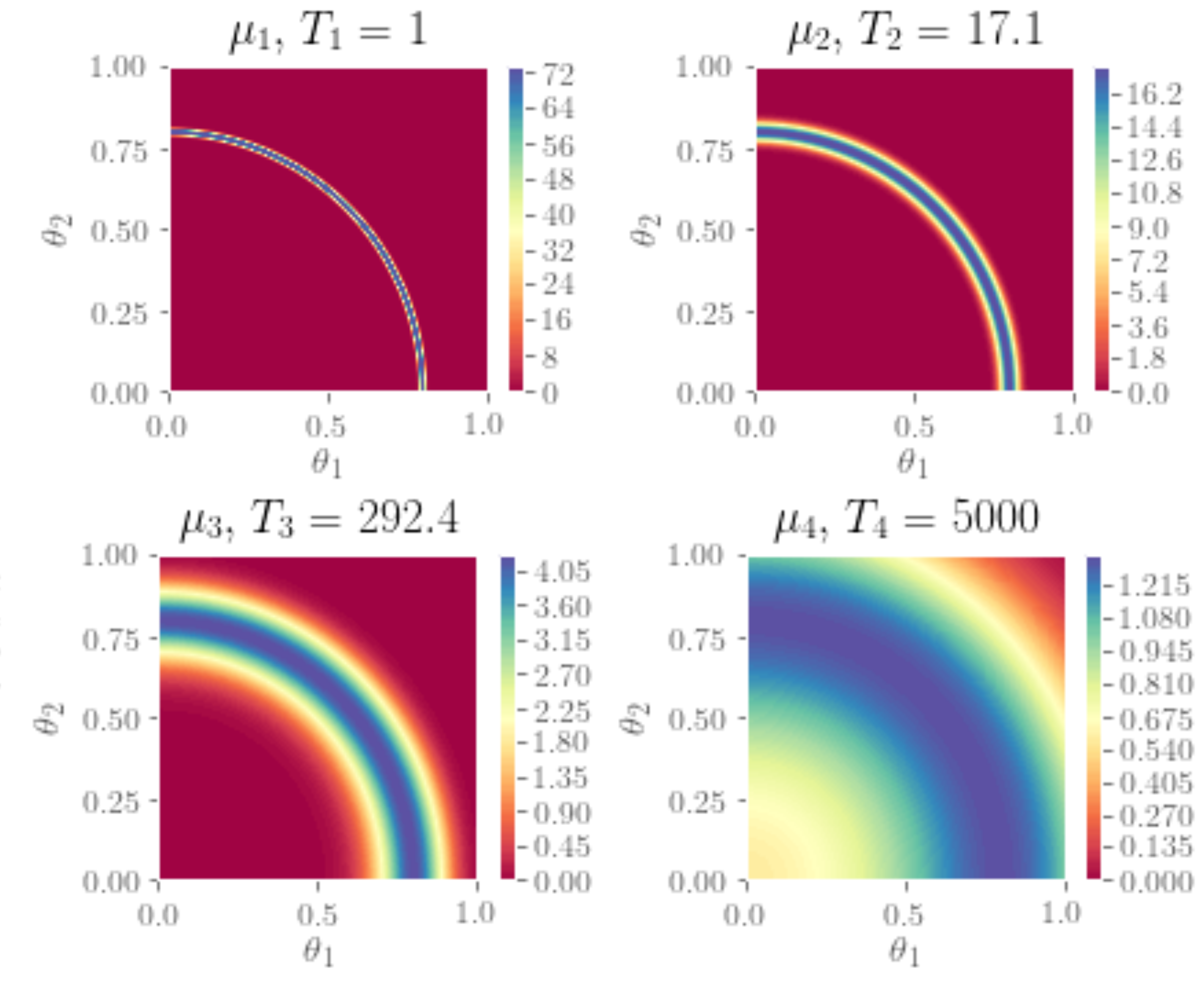
Figure 2: Tempered densities (with $T_{1}=1,\ T_{2}=17.1,\ T_{3}=292.4,\ T_{4}=5000$) for the density concentrated around a quarter circle-shaped manifold example. As we can see, the density becomes less concentrated as the temperature increases, which allows us to use RWM proposals with larger step sizes.

We aim at estimating $\hat{\mathcal{Q}}_{i}=\mathbb{E}_{\mu}[\theta_{i}]\approx\hat{\theta}_{i}$, for $i=1,2$. For the tempered algorithms (PT, PSDPT, UGPT, and WGPT), we consider $K=4$ temperatures and choose $T_{4}=5000$, so that the tempered density $\pi_{4}$ becomes sufficiently simple to explore the target distribution. This gives $T_{1}=1,T_{2}=17.1,T_{3}=292.4,T_{4}=5000$. We compare the quality of our algorithms by examining the variance of the estimators $\hat{\theta}_{i},$ $i=1,2$ computed over $N_{\text{runs}}=100$ independent MCMC runs of each algorithm. For the tempered algorithms, each estimator is obtained by running the inversion experiment for $N=25,000$ samples per run, discarding the first 20% of the samples (5000) as a burn-in. Accordingly, we run the single-chain random walk Metropolis algorithm for $N_{\mathrm{RWM}}=KN=100,000$ iterations, per run, and discard the first 20% of the samples obtained with the RWM algorithm (20,000) as a burn-in.

The untempered RWM algorithm uses Gaussian proposals with covariance matrix $\Sigma_{\mathrm{RWM}}=\rho_{1}^{2}I_{2\times 2},$ where $I_{2\times 2}$ is the identity matrix in $\mathbb{R}^{2\times 2}$, and $\rho^{2}_{1}=0.022$ is chosen in order to obtain an acceptance rate of around 0.23. For the tempered algorithms (i.e., PT, PSDPT, and both versions of GPT), we use $K=4$ RWM kernels $p_{k}$, $k=1,2,3,4$, with proposal density $q_{\mathrm{prop},k}(\theta^{(n)}_{k},\cdot)=\mathcal{N}(\theta_{k}^{(n)},\rho_{k}^{2}I_{2\times 2})$, where $\rho_{k}$ is shown in Table 1. This choice of $\rho_{k}$ gives an acceptance rate for each chain of around 0.23. Notice that $\rho_{1}$ corresponds to the “step-size” of the single-temperature RWM algorithm.

	$k=1$	$k=2$	$k=3$	$k=4$
$\rho_{k}$	0.022	0.090	0.310	0.650

Table 1: Step size of the RWM proposal distribution for the manifold experiment.

Experimental results for the ergodic run are shown in Table 2. We can see how both GPT algorithms provide a gain over RWM, PT and PSDPT algorithms, with the WGPT algorithm providing the largest gain. Scatter plots of the samples obtained with each method are presented in Figure 3. Here, the subplot titled “WGPT” (bottom row, middle) corresponds to weighted samples from $\bm{\mu}_{\textrm{W}}$, with weight $\hat{w}$ as in (82), while the one titled “WGPT (inv)” (bottom row, right) corresponds to samples from $\bm{\mu}_{\mathrm{W}}$ without any post-processing. Notice how the samples from the latter concentrates over a thicker manifold, which in turn makes the target density easier to explore when using state-dependent Markov transition kernels.

	Mean		MSE		MSE${}_{\mathrm{RWM}}/$MSE
	$\hat{\theta}_{1}$	$\hat{\theta}_{2}$	$\hat{\theta}_{1}$	$\hat{\theta}_{2}$	$\hat{\theta}_{1}$	$\hat{\theta}_{2}$
RWM	0.50996	0.50657	0.00253	0.00261	1.00	1.00
PT	0.50978	0.51241	0.00024	0.00021	10.7	11.0
PSDPT	0.50900	0.50956	0.00027	0.00026	9.53	10.2
UGPT	0.50986	0.50987	0.00016	0.00016	16.1	16.4
WGPT	0.51062	0.50838	0.00015	0.00014	16.9	18.4

Table 2: Results for the density concentrated around a circle-shaped manifold experiment. As we can see, both GPT algorithms provide an improvement over PT, PSDPT and RWM. The computational cost is comparable across all algorithms.

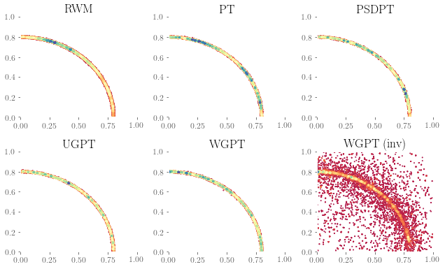
Figure 3: Scatter-plots of the samples from $\mu$ obtained with each algorithm on a single run. Top, from left to right: random walk Metropolis, PT and PSDPT. Bottom, from left to right: UGPT, WGPT (after re-weighting the samples), and WGPT, before re-weighting the samples.

5.4 Multiple source elliptic BIP

We now consider a slightly more challenging problem, for which we try to recover the probability distribution of the location of a source term in a Poisson equation (Eq. (144)), based on some noisy measured data. Let $(\Theta,\mathcal{B}(\Theta),\mu_{\mathrm{pr}})$ be the measure space, set $\Theta=\bar{D}\mathrel{\mathop{\mathchar 58\relax}}=[0,1]^{2}$, with Lebesgue (uniform) measure $\mu_{\mathrm{pr}},$ and consider the following Poisson’s equation with homogeneous boundary conditions:

$$\begin{cases}\Delta u(x,\theta)=f(x,\theta),&x\in D,\ \theta\in\Theta,\\ u(x,\theta)=0,&x\in\partial D.\end{cases}$$ (144)

Such equation can model, for example, the electrostatic potential $u\mathrel{\mathop{\mathchar 58\relax}}=u(x,\theta)$ generated by a charge density $f(x,\theta)$ depending on an uncertain location parameter $\theta\in\Theta$. Data $y$ is recorded on an array of $64\times 64$ equally-spaced points in $D$ by solving (144) with a forcing term given by

$$f(x)=\sum_{i=1}^{4}e^{-1000[(x_{1}-s^{(i)}_{1})^{2}+(x_{2}-s^{(i)}_{2})^{2}]},$$ (145)

where the true source locations $s^{(i)},\ i=1,2,3,4,$ are given by $s^{(1)}=(0.2,0.2),\ s^{(2)}=(0.2,0.8),\ s^{(3)}=(0.8,0.2),$ and $s^{(4)}=(0.8,0.8)$. Such data is assumed to be polluted by an additive Gaussian noise with distribution $\mathcal{N}(0,\eta^{2}I_{64\times 64})$, with $\eta=3.2\times 10^{-6}$, (which corresponds to a $1$% noise) and where $I_{64\times 64}$ is the 64-dimensional identity matrix. Thus, we set $(Y,\left\|\cdot\right\|_{Y})=(\mathbb{R}^{64\times 64},\left\|\cdot\right\|)$, with $\left\|A\right\|=(64\eta)^{-2}\left\|A\right\|^{2}_{F}$, for some arbitrary matrix $A\in\mathbb{R}^{64\times 64},$ where $\left\|\cdot\right\|_{F}$ is the Frobenius norm. We assume a misspecified model where we only consider a single source in Eq. (145). That, is, we construct our forward operator ${\mathcal{F}}\mathrel{\mathop{\mathchar 58\relax}}\Theta\mapsto Y$ by solving (144) with a source term given by

$$f(x,\theta)=e^{-1000[(x_{1}-\theta_{1})^{2}+(x_{2}-\theta_{2})^{2}]}.$$ (146)

In this particular setting, this leads to a posterior distribution with four modes since the prior density is uniform in the domain and the likelihood has a local maximum whenever $(\theta_{1},\theta_{2})=(s_{1}^{(i)},s_{2}^{(i)}),\ i=1,2,3,4$. The Bayesian inverse problem at hand can be understood as sampling from the posterior measure $\mu$, which has a density with respect to the prior $\mu_{\mathrm{pr}}=\mathcal{U}(\bar{D})$ given by

$$\pi(\theta)=\frac{1}{Z}\exp\left(-\frac{1}{2}\left\|y-\mathcal{F}(\theta)\right\|^{2}_{\Sigma}\right),$$ (147)

for some (intractable) normalization constant $Z$ as in (10). We remark that the solution to (144) with a forcing term of the form of (146) is approximated using a second-order accurate finite difference approximation with grid-size $h=1/64$ on each spatial component.

The difficulty in sampling from the current BIP arises from the fact that the resulting posterior $\mu$ is multi-modal and the number of modes is not known apriori (see Figure 4).

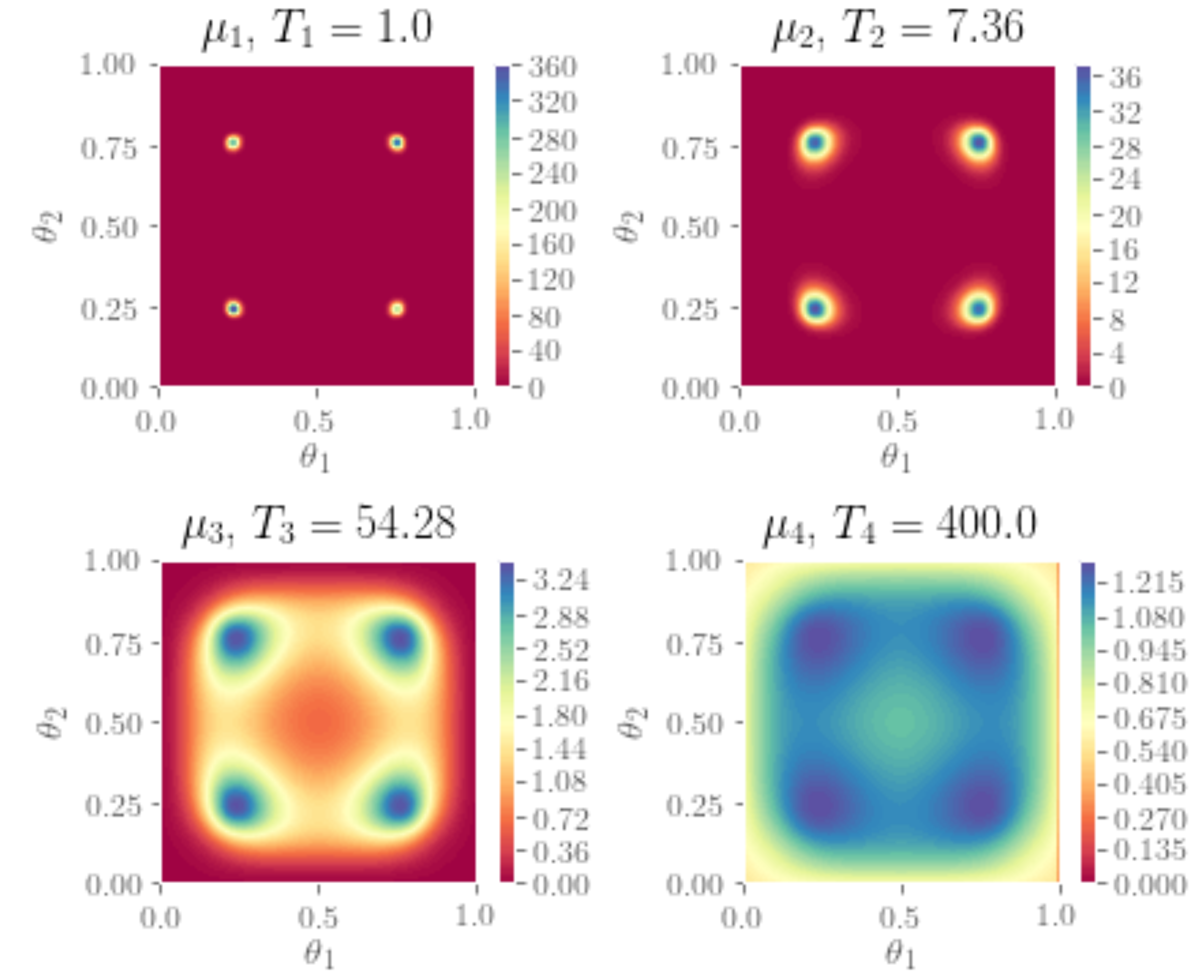
Figure 4: True tempered densities for the elliptic BIP example. Notice that the density is not symmetric, due to the additional random noise.

We follow a similar experimental setup to the previous example, and aim at estimating $\hat{\mathcal{Q}}_{i}=\mathbb{E}_{\mu}[\theta_{i}]\approx\hat{\theta}_{i}$, for $i=1,2$. We use $K=4$ temperatures and $N_{\text{runs}}=100$. For the PT, PSDPT and GPT algorithms, four different temperatures are used, with $T_{1}=1,\ \ T_{2}=7.36,\ \ T_{3}=54.28,$ and $T_{4}=400$. For each run, we obtain $N=25,000$ samples with the PT, PSDPT, and both GPT algorithms, and $N=100,000$ samples with RWM, discarding the first 20% of the samples in both cases (5000, 20000, respectively) as a burn-in. On each of the tempered chains, we use RWM proposals, with step-sizes shown in table 3. This choice of step size provides an acceptance rate of about 0.24 across all tempered chains and all tempered algorithms. For the single-temperature RWM run, we choose a larger step size ($\rho_{\mathrm{RWM}}=0.16$) so that the RWM algorithm is able to explore the whole distribution. Such a choice, however, provides a smaller acceptance rate of about 0.01 for the single-chain RWM.

Experimental results are shown in Table 4. Once again, we can see how both GPT algorithms provide a gain over RWM and both variations of the PT algorithm, with the WGPT algorithm providing a larger gain. Scatter-plots of the obtained samples are shown in Figure 4.

	$k=1$	$k=2$	$k=3$	$k=4$
$\rho_{k,\mathrm{Tempered}}$	0.030	0.100	0.400	0.600
$\rho_{k,\mathrm{RWM}}$	0.160	-	-	-

Table 3: Step size of the RWM proposal distribution for the elliptic BIP experiment.

	Mean		MSE		MSE${}_{\mathrm{RWM}}/$MSE
	$\theta_{1}$	$\theta_{2}$	$\theta_{1}$	$\theta_{2}$	$\theta_{1}$	$\theta_{2}$
RWM	0.48509	0.51867	0.00986	0.01270	1.00	1.00
PT	0.48731	0.50758	0.00042	0.00036	23.0	29.2
PSDPT	0.48401	0.50542	0.00079	0.00099	12.4	10.7
UGPT	0.48624	0.50620	0.00038	0.00027	25.9	38.2
WGPT	0.48617	0.50554	0.00025	0.00023	38.6	44.9

Table 4: Results for the elliptic BIP problem. The computational cost is comparable across all algorithms, given that the cost of each iteration is dominated by the cost of solving the underlying PDE.

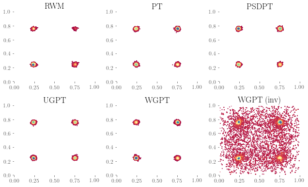
Figure 5: Scatterplots of the samples from $\mu$ obtained with different algorithms on a single run. Top, from left to right: random walk Metropolis, PT and PSDPT. Bottom, from left to right: UGPT, WGPT (after re-weighting the samples), and WGPT, before re-weighting the samples. As we can see, WGPT (before re-weighting) is able to "connect" the parameter space.

5.5 1D wave source inversion

We consider a small variation of example 5.1 in motamed2019wasserstein . Let $(\Theta,\mathcal{B}(\Theta),\mu_{\mathrm{pr}})$ be a measure space, with $\Theta=[-5,5]$ and uniform (Lebesgue) measure $\mu_{\mathrm{pr}}$, and let $I=(0,T]$ be a time interval. Consider the following Cauchy problem for the 1D wave equation:

$$\begin{cases}u_{tt}(x,t,\theta)-u_{xx}(x,t,\theta)=0,&(x,t,\theta)\in\mathbb{R}\times I\times\Theta,\\ u(x,0,\theta)=h(x,\theta),&(x,t,\theta)\in\mathbb{R}\times\{0\}\times\Theta,\\ u_{t}(x,0,\theta)=0,&(x,t,\theta)\in\mathbb{R}\times\{0\}\times\Theta.\\ \end{cases}$$ (148)

Here, $h(x,\theta)$ acts as a source term generating a initial wave pulse. Notice that Equation (148) can be easily solved using d’Alembert’s formula, namely

$$u(x,t,\theta)=\frac{1}{2}\left(h(x-t,\theta)+h(x+t,\theta)\right).$$ (149)

Synthetic data $y$ is generated by solving Equation (148) with initial data

$$h(x,\theta_{1},\theta_{2}) =\frac{1}{2}\left(e^{-100(x-\theta_{1}-0.5)^{2}}+e^{-100(x-\theta_{1})^{2}}\right.$$ (150)

$$\left.+e^{-100(x-\theta_{1}+0.5)^{2}}+e^{-100(x-\theta_{2}-0.5)^{2}}\right.$$ (151)

$$\left.+e^{-100(x-\theta_{2})^{2}}+e^{-100(x-\theta_{2}+0.5)^{2}}\right),$$ (152)

with $\theta_{1}=-3,\theta_{2}=3$ and observed at $N_{R}=11$ equally-spaced receiver locations between $R_{1}=-5$ and $R_{2}=5$ on $N_{T}=1000$ time instants between $t=0$ and $T=5$. The signal recorded by each receiver is assumed to be polluted by additive Gaussian noise $\mathcal{N}(0,\eta^{2}I_{1000\times 1000})$, with $\eta=0.01$, which corresponds to roughly 1% noise. We set $(Y,\left\|\right\|_{Y})=(\mathbb{R}^{11\times 1000},\left\|\cdot\right\|_{\Sigma}),$ with

$$\left\|A\right\|_{\Sigma}^{2}=(\sqrt{N_{R}}\eta)^{-2}\sum_{i=1}^{N_{R}}\sum_{j=1}^{N_{T}}A_{i,j}^{2},$$

$A\in\mathbb{R}^{11\times 1000}$. Once again, we assume a misspecified model where we construct our forward operator ${\mathcal{F}}\mathrel{\mathop{\mathchar 58\relax}}\Theta\mapsto Y$ by solving (148) with a source term given by

$$h(x,\theta) =\left(e^{-100(x-\theta-0.5)^{2}}\right.$$ (153)

$$\left.+e^{-100(x-\theta)^{2}}+e^{-100(x-\theta+0.5)^{2}}\right).$$ (154)

The Bayesian inverse problem at hand can be understood as sampling from the posterior measure $\mu$, which has a density with respect to the prior $\mu_{\mathrm{pr}}=\mathcal{U}([-5,5])$ given by

$$\pi(\theta) =\frac{1}{Z}\exp\left(-\frac{1}{2}\left\|y-\mathcal{F}(\theta)\right\|^{2}_{\Sigma}\right)$$ (155)

$$=\frac{1}{Z}\exp\left(-\Phi(\theta;y)\right),$$ (156)

for some (intractable) normalization constant $Z$ as in (10). The difficulty in solving this BIP comes from the high multi-modality of the potential $\Phi(\theta;y)$, as it can be seen in Figure 6. This, shape of $\Phi(\theta;y)$ makes the posterior difficult to explore using local proposals.

Figure 6: Multi-modal potential for the Cauchy problem. Notice the minima around $\theta=-3$ and $\theta=3$.

In this case, we consider $K=5$, and set $T_{1}=1,\ \ T_{2}=5,\ \ T_{3}=25,$ $T_{4}=125$ and $T_{5}=625$. Notice that from Figure 1, the computational cost per sample is dominated by the evaluation of (155) for values of $K\leq 6$. Once again, we obtain $N=25,000$ samples with the PT, PSDPT, and both GPT algorithms, and $N=125,000$ samples with RWM, discarding the first 20% of the samples in both cases (5000, 25000, respectively) as a burn-in. On each of the tempered chains, we use RWM proposals, with step-sizes shown in table 5. This choice of step size provides an acceptance rate of about 0.4 across all tempered chains and all tempered algorithms. The choice of step-size for the RWM algorithm is done in such a way that it can "jump" modes, which are at distance of roughly 1/2.

We consider $\mathcal{Q}=\theta$ as a quantity of interest. Experimental results are shown in Table 6. Once again, we can see how both GPT algorithms provide a gain over RWM and both variations of the PT algorithm, with the WGPT algorithm providing the largest gain. Notice that, given the high muti-modality of the posterior at hand, the simple RWM algorithm is not well-suited for this type of distribution, as it can be seen from its large variance; this suggests that the RWM usually gets "stuck" at one mode of the posterior. Notice that, intuitively, due to the symmetric nature of the potential, one would expect the true mean of $\theta$ to be close to 0. This value was computed by means of numerical integration and is given by $\mathbb{E}_{\mu}[\theta]=0.08211$.

	$k=1$	$k=2$	$k=3$	$k=4$	$k=5$
$\rho_{k,\mathrm{Tempered}}$	0.02	0.05	0.10	0.50	2.0
$\rho_{k,\mathrm{RWM}}$	0.5	-	-	-	-

Table 5: Step size of the RWM proposal distribution for the Cauchy BIP experiment.

	Mean	MSE	MSE${}_{\mathrm{RWM}}/$MSE
RWM	-0.10120	9.36709	1.000
PT	0.05118	0.03681	254.5
PSDPT	0.15840	0.21701	43.20
UGPT	0.08976	0.03032	308.9
WGPT	0.06149	0.02518	372.0

Table 6: Results for the 1D Cauchy BIP problem. The computational cost is comparable across all algorithms.

5.6 Acoustic wave source inversion

We consider a more challenging problem, for which we try to recover the probability distribution of the spatial location of a (point-like) source term, together with the material properties of the medium, on an acoustic wave equation (Eq. (157)), based on some noisy measured data. We begin by describing the mathematical model of such wave phenomena. Let $(\Theta,\mathcal{B}(\Theta),\mu_{\mathrm{pr}})$ be the measure space , with Lebesgue (uniform) measure $\mu_{\mathrm{pr}}$, set $\bar{D}\mathrel{\mathop{\mathchar 58\relax}}=[0,3]\times[0,2],$ $\partial D=\bar{\Gamma}_{N}\cup\bar{\Gamma}_{\mathrm{Abs}},\ \mathring{\Gamma}_{\mathrm{N}}\cap\mathring{\Gamma}_{\mathrm{Abs}}=0,$ $|\Gamma_{\mathrm{N}}|,|\Gamma_{\mathrm{Abs}}|>0,$ and define $\Theta=D\times\Theta_{\alpha}\times\Theta_{\beta},$ where $\Theta_{\alpha}=[6,14]$, $\Theta_{\beta}=[4500,5500]$. Here, we are considering a rectangular spatial domain $D$, with the top boundary denoted by $\Gamma_{\mathrm{N}}$ and the side and bottom boundaries denoted by $\Gamma_{\mathrm{Abs}}$. Lastly, let $\theta\mathrel{\mathop{\mathchar 58\relax}}=(s_{1},s_{2},\alpha,\beta)\in\Theta$. Consider the following acoustic wave equation with absorbing boundary conditions:

$$\begin{cases}\alpha^{2}u_{tt}-\nabla\cdot(\beta^{2}\nabla u)=f,&\text{in }D\times(0,T)\times\Theta,\\ u=u_{t}=0,&\text{in }D\times\{0\}\times\Theta,\\ \beta^{2}\nabla u\cdot\hat{n}=0,&\text{on }\Gamma_{\mathrm{N}}\times(0,T)\times\Theta,\\ \beta^{2}\nabla u\cdot\hat{n}=-\alpha\beta u_{t},&\text{on }\Gamma_{\mathrm{Abs}}\times(0,T)\times\Theta,\end{cases}$$ (157)

where $u=u(x,t,\theta)$, and $f=f(x,t,\theta)$. Here the boundary condition on the top boundary $\Gamma_{\mathrm{N}}$ corresponds to a Neumann boundary condition, while the boundary condition on $\Gamma_{\mathrm{Abs}}$ corresponds to the so-called absorbing boundary condition, a type of artificial boundary condition used to minimize reflection of wave hitting the boundary. Data $y\in Y$ is obtained by solving Equation $\eqref{Eq:acoustic}$ with a force term given by

$$f(x,t,\theta) =10^{11}e^{-\frac{1}{2\cdot 0.1^{2}}\left[\left(x_{1}-s_{1}\right)^{2}+\left(x_{2}-s_{2}\right)^{2}\right]}$$ (158)

$$\times(1-2\cdot 1000\pi^{2}t^{2})e^{-2\cdot 1000^{2}\pi^{2}t^{2}},$$ (159)

with a true set of parameters $\Theta\ni\theta^{*}\mathrel{\mathop{\mathchar 58\relax}}=(s_{1},s_{2},\alpha,\beta)$ given by $s_{1}=1.5,s_{2}=1.0,\alpha=10,\beta=5000$, and observed on $N_{R}=3$ different receiver locations $R_{1}=(1.0,2.0),R_{2}=(1.5,2.0),R_{3}=(2.0,2.0)$ at $N_{T}=117$ equally-spaced time instants between $t=0$ and $t=0.004$. In physical terms, the parameters $s_{1},s_{2}$ represent the source location, while the parameters $\alpha,\beta$ are related to the material properties of the medium. Notice that, on a slight abuse of notation, we have used the symbol $\pi$ to represent the number $3.14159\dots$ in equation (158) and it should not be confused with the symbol for density. The data measured by each receiver is polluted by additive Gaussian noise $\mathcal{N}(0,\eta^{2}I_{117\times 117})$, with $\eta=0.013$, which corresponds to roughly a 2% noise. Thus, we have that $(Y,\left\|\cdot\right\|_{Y})=(\mathbb{R}^{3\times 117},\left\|\cdot\right\|_{\Sigma}),$ where $\left\|A\right\|_{\Sigma}^{2}\mathrel{\mathop{\mathchar 58\relax}}=(\sqrt{N_{R}}\eta)^{-2}\sum_{i=1}^{N_{R}}\sum_{j=0}^{N_{T}}A_{i,j}^{2}$. Thus, the forward mapping operator $\mathcal{F}\mathrel{\mathop{\mathchar 58\relax}}\Theta\mapsto Y$ can be understood as the numerical solution of Equation (157) evaluated at 117 discrete time instants at each of the 3 receiver locations. Such a numerical approximation is obtained by the finite element method using piece-wise linear elements and the time stepping is done using a Forward Euler scheme with sufficiently small time-steps to respect the so-called Courant-Friedrichs-Lewy condition quarteroni2009numerical . This numerical solution is implemented using the Python library FEniCS logg2012automated , using 40$\times 40$ triangular elements. The Bayesian inverse problem at hand can thus be understood as sampling from the posterior measure $\mu$, which has a density with respect to the prior $\mu_{\mathrm{pr}}=\mathcal{U}(\Theta)$ given by

$$\pi(\theta)=\frac{1}{Z}\exp\left(-\frac{1}{2}\left\|y-\mathcal{F}(\theta)\right\|^{2}_{\Sigma}\right).$$ (160)

The previous BIP presents two difficulties; on the one hand, Equation (157) is, typically, expensive to solve, which in turn translates into expensive evaluations of the posterior density. On the other, the log-likelihood has an extremely complicated structure, which in turn makes its exploration difficult. This can be seen in Figure 7, where we plot of the log-likelihood for different source locations $(s_{1},s_{2})$ and for fixed values of the material properties $\alpha=10,\beta=5000.$ More precisely, we plot $\tilde{\Phi}((s_{1},s_{2});y)\mathrel{\mathop{\mathchar 58\relax}}=-\frac{1}{2}\left\|y-{\mathcal{F}}(s_{1},s_{2},10,5000)\right\|^{2}_{\Sigma}$ on a grid of $100\times 100$ equally spaced points $(s_{1},s_{2})$ in $D$. It can be seen that, even though the log-likelihood has a clear peak around the true value of $(s_{1},s_{2})$, there are also regions of relatively high concentration of log-probability, surrounded by regions with a significantly smaller log-probability, making it a suitable problem for our setting.

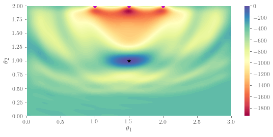
Figure 7: Plot of the log-likelihood for different values of $s_{1}$, $s_{2}$ and fixed values of $\alpha=10$ and $\beta=5000$. The magenta points represent the reciever locations $R_{1},R_{2},R_{3}$. The black point represents the true location of the source $(s_{1},s_{2})=(1.5,1.0)$.

Following the same set-up of previous experiments, we aim at estimating $\hat{\mathcal{Q}}_{i}=\mathbb{E}_{\mu}[\theta_{i}]\approx\hat{\theta}_{i}$, for $i=1,2$. Once again, we consider $K=4$ temperatures for the tempered algorithms (PT, PSDPT, UGPT, and WGPT), and set temperatures to $T_{1}=1,T_{2}=7.36,T_{3}=54.28,$ $T_{4}=400$. We compare the quality of our algorithms by examining the variance of the estimators $\hat{\theta}_{i},$ $i=1,2$ computed over $N_{\text{runs}}=50$ independent MCMC runs of each algorithm. For each run, we run the tempered algorithms obtaining $N=7,000$ samples, discarding the first 20% of the samples (1400) as a burn-in. For the RWM algorithm, we run the inversion experiment for $N_{\mathrm{RWM}}=KN=28,000$ iterations, and discard the first 20% of the samples obtained (5600) as a burn-in.

Each individual chain is constructed using Gaussian RWM proposals $q_{\mathrm{prop},k}(\theta^{n}_{k},\cdot)=\mathcal{N}(\theta^{n}_{k},\mathcal{C}_{k})$, $k=1,2,3,4$, with covariance $\mathcal{C}_{k}$ described in Table 7. The covariance is tuned in such a way that the acceptance rate of each chain is around 0.2. The variance of the estimators obtained with each method is presented in Table 8. Once again, our GPT algorithms outperform all other tested methods for this particular setting. In particular, our methods provide huge computational gains when compared to RWM and the PSDPT algorithm of lkacki2016state , as well as some moderate computational gains when compared to the standard PT.

	$\mathcal{C}^{1/2}_{k,\mathrm{Tempered}}$	$\mathcal{C}^{1/2}_{k,\mathrm{RWM}}$
$k=1$	$\mathrm{Diag}(0.01,0.01,0.2,5)$	$\mathrm{Diag}(0.02,0.02,0.2,5)$
$k=2$	$\mathrm{Diag}(0.06,0.06,0.4,14)$	-
$k=3$	$\mathrm{Diag}(0.3,0.3,0.6,20)$	-
$k=4$	$\mathrm{Diag}(1,1,1,50)$	-

Table 7: Step size of the RWM proposal distribution for the acoustic BIP experiment. Here $\mathrm{Diag}(d_{1},d_{2},\dots,d_{N})$ is to be understood as the $N\times N$ diagonal matrix with entries $d_{1},d_{2},\dots,d_{N}$.

	Mean		Var		Var${}_{\mathrm{RWM}}/$Var
	$s_{1}$	$s_{2}$	$s_{1}$	$s_{2}$	$s_{1}$	$s_{2}$
RWM	1.33801	1.54293	$9.86\times 10^{-1}$	8.21$\times 10^{-2}$	1.000000	1.000
PT	1.50121	1.00829	$6.61\times 10^{-6}$	$2.77\times 10^{-4}$	149136.1	296.2
PSDPT	1.39775	1.23119	$2.48\times 10^{-1}$	$6.54\times 10^{-2}$	3.900000	1.200
UGPT	1.50177	1.00711	$2.72\times 10^{-6}$	$2.38\times 10^{-4}$	361744.5	345.0
WGPT	1.50174	1.00601	$2.08\times 10^{-6}$	$1.46\times 10^{-4}$	472133.2	558.6

Table 8: Results for the acoustic BIP problem. Once again, we can see that both GPT algorithm provide an improvement over RWM, PT and PSDPT. The computational cost is comparable across all algorithms, given that the cost of each iteration is dominated by the cost of solving the underlying PDE.

5.7 High-dimensional acoustic wave inversion

Lastly, we present a high-dimensional example for which we try to invert for the material properties $\beta^{2}$ in (157). For simplicity, we will consider fixed values of $\alpha=1,$ $s_{1}=1.5,$ and $s_{2}=1$. In this case, we set $\beta^{2}=10+\hat{\beta}^{2}(x)$, where $\hat{\beta}(x)$ is taken to be a realization of a random field discretized on a mesh of $N_{x}\times N_{y}$ triangular elements. This modeling choice ensures that $\beta^{2}$ is lower bounded. In this case, we will invert for the nodal values of (the finite element discretization of) $\hat{\beta}$, which will naturally result in a high-dimensional problem. We remark that one is usually interested in including the randomness in $\beta^{2}$, instead of $\hat{\beta}$; however, we purposely choose to do so to induce an explicitly multi-modal posterior, and as such, to better illustrate the advantages of our proposed methods when sampling from these types of distributions.

We begin by formalizing the finite-element discretization of the parameter space (see e.g., bui2016fem for a more detailed discussion).

Let $\bar{D}=[0,3]\times[0,2],$ denote the physical space of the problem and let $V_{h}$ be a finite-dimensional subspace of $L_{2}(D)$ arising from a given finite element discretization. We write the finite element approximation $\hat{\beta}_{h}\in V_{h}$ of $\hat{\beta}$ as

$$\hat{\beta}(x)\approx\hat{\beta}_{h}(x)=\sum_{n=1}^{N_{\text{v}}}b_{n}\phi_{n}(x),$$

where $\{\phi\}_{n=1}^{N_{\text{v}}}$ are the Lagrange basis functions corresponding to the nodal points $\{x_{n}\}_{n=1}^{N_{\text{v}}}$, $(b_{1},\dots,b_{N_{\text{v}}})^{T}=\mathrel{\mathop{\mathchar 58\relax}}\theta\in\mathbb{R}^{N_{\text{v}}}$ is the set of nodal parameters and $N_{\text{v}}$ corresponds to the number of vertices used in the FE discretization. Thus, the problem of inferring the distribution of $\beta$ given some data $y$, can be understood as inferring the distribution of $\theta$ given $y$. For our particular case, we will discretize $D$ using $28\times 28$ (non-overlapping) piece-wise linear finite elements, which results in $N_{\text{v}}=841$ and as such $\Theta=\mathbb{R}^{841}$. We consider a Gaussian prior $\mu_{\mathrm{pr,\infty}}=\mathcal{N}(0,\mathcal{A}^{-2})$, where $\mathcal{A}$ is a differential operator acting on $L_{2}(D)$ of the form

$$\mathcal{A}\mathrel{\mathop{\mathchar 58\relax}}=-a\nabla\cdot(H\nabla)+dI,\quad a,d>0,$$ (161)

together with Robin boundary conditions $\nabla(\cdot)\cdot\hat{n}+\sqrt{ad}(\cdot)=0$, where, following VillaPetraGhattas21 , $H$ is taken of the form

$$H\mathrel{\mathop{\mathchar 58\relax}}=\begin{pmatrix}e_{1}\sin^{2}(\ell)+e_{2}\cos^{2}(\ell)&&&(e_{1}-e_{2})\sin(\ell)\cos(\ell)\\ (e_{1}-e_{2})\sin(\ell)\cos(\ell)&&&e_{1}\cos^{2}(\ell)+e_{2}\sin^{2}(\ell)\end{pmatrix}.$$ (162)

Here $H$ models the spatial anisotropy of a Gaussian Random field sampled from $\mu_{\mathrm{pr,\infty}}$. It is known that for a two-dimensional (spatial) space, the covariance operator $\mathcal{A}^{-2}$ is symmetric and trace-class bui2016fem , and as such, the (infinite-dimensional) prior measure is well-defined. Thus, we set

$$\hat{\beta}(x)\sim{\mu}_{\mathrm{pr,\infty}},$$ (163)

which in turn induces the discretized prior:

$${\hat{\beta}_{h}}(x)\sim\mu_{\mathrm{pr}}\mathrel{\mathop{\mathchar 58\relax}}=\mathcal{N}(0,\mathcal{A}_{h}^{-2}),$$ (164)

where $\mathcal{A}_{h}^{-2}$ is a finite-element approximation of $\mathcal{A}$ using $28\times 28$ (non-overlapping) piece-wise linear finite elements. Samples from $\mu_{\mathrm{pr}}$ are obtained using the FEniCS package logg2012automated and the hIPPYlib library VillaPetraGhattas21 .

We follow an approach similar to our previous example. We collect data $y\in Y$ by solving Equation (157) with a force term given by (158) and a true field $\hat{\beta}^{*}_{h}\sim\mu_{\mathrm{pr}}$ with $a=0.1$, $d=0.5$, $\ell=\pi/4$, $e_{1}=2$ and $e_{2}=0.5$. Such a realization of $\hat{\beta}^{*}_{h}$ is shown in Figure 8.

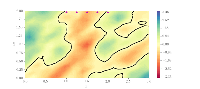
Figure 8: True field $\hat{\beta}^{*}_{h}(x)$. Notice the anisotropy on the field. The magenta points represent the receiver locations. The black line represents the zero-level set of the field.

Furthermore, data is observed at $N_{R}=5$ different receiver locations $R_{1}=(1.0,2.0),R_{2}=(1.25,2.0),R_{3}=(1.5,2.0),R_{4}=(1.75,2.0)$, and $R_{5}=(2.0,2.0)$ at $N_{T}=600$ equally-spaced time instants between $t=0$ and $t=0.6$. The data measured by each receiver is polluted by an (independent) additive Gaussian noise $\eta\sim\mathcal{N}(0,\sigma_{\mathrm{noise}}^{2}I_{600\times 600})$, with $\sigma=0.021$, which corresponds to roughly a 0.5% noise. Thus, we have that $(Y,\left\|\cdot\right\|_{Y})=(\mathbb{R}^{5\times 600},\left\|\cdot\right\|_{\Sigma})$. Similarly as in Section 5.6, the forward mapping operator $\mathcal{F}\mathrel{\mathop{\mathchar 58\relax}}\Theta\mapsto Y$ can be understood as the numerical solution of Equation (157) evaluated at 600 discrete time instants at each of the 5 receiver locations. Numerical implementation follows a similar set-up as in Section 5.6, however, for simplicity, we use $28\times 28$ triangular elements to approximate the forward operator ${\mathcal{F}}$. The Bayesian inverse problem at hand can thus be understood as sampling from the posterior measure $\mu$, which has a Radon-Nikodym derivative with respect to the prior $\mu_{\mathrm{pr}}$ given by

$$\pi(\theta)=\frac{\mathrm{d}\mu}{\mathrm{d}\mu_{\mathrm{pr}}}(\theta)=\frac{1}{Z}\exp\left(-\frac{1}{2}\left\|y-\mathcal{F}(\theta)\right\|^{2}_{\Sigma}\right).$$ (165)

The previous BIP has several difficulties; clearly, it is a high-dimensional posterior. Furthermore, just as in the previous example, the underlying mathematical model for the forward operator is a costly time-dependent PDE. By choosing to invert for $\hat{\beta}_{h}\sim\mu_{\mathrm{pr}}$ (instead of $\beta_{h}^{2}\approx\beta^{2}$), and since $\mu_{\mathrm{pr}}$ is centered at zero, we induce a multi-modal posterior, indeed, if the posterior concentrates around $\hat{\beta}^{*}_{h}$ it will also have peaks at any other $\hat{\beta}^{j}$ obtained by flipping the sign of $\hat{\beta}^{*}_{h}$ in a concentrated region separated by the zero level set of $\hat{\beta}^{*}_{h}$ (we identify 7 regions in Figure 8). This can be seen in Figure 9, where we plot 4 posterior samples $\hat{\beta}_{h}\sim\mu$. Notice the change in sign between some regions. Lastly, as a quantities of interest, we will consider $\mathcal{Q}_{1}=\int_{D}\exp(\hat{\beta}(x))\mathrm{d}x$ and $\mathcal{Q}_{2}=\exp(\hat{\beta}(1.5,1))$. We remark that, although these quantities of interest do not have any meaningful physical interpretation, they are, however, affected by the multi-modality of the posterior, and as such, well suited to exemplify the capabilities of our method.

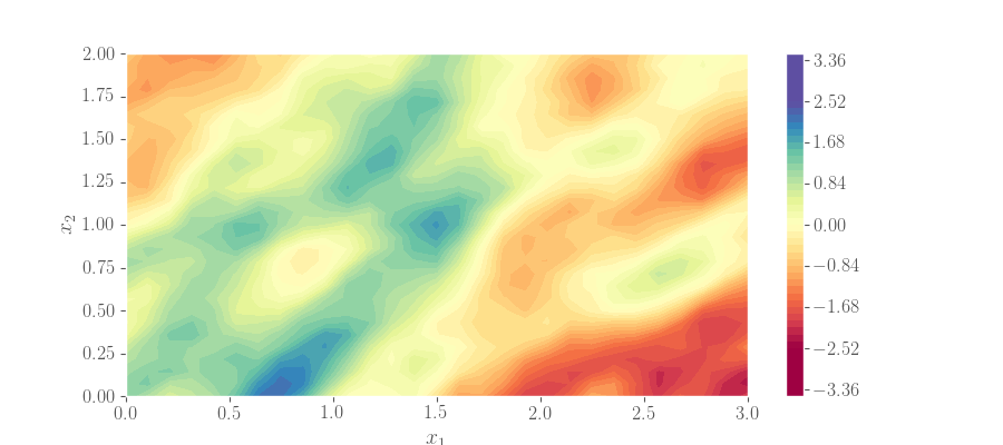
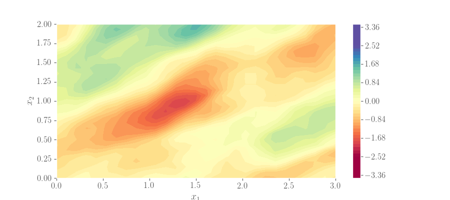
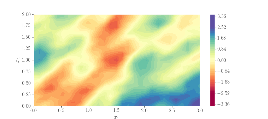
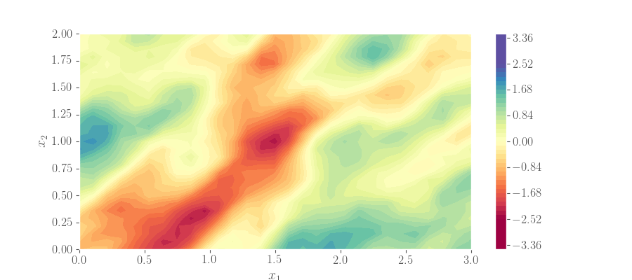
Figure 9: Posterior samples $\hat{\beta}_{h}\sim\mu$ obtained with the UW GPT algorithm. Notice the resemblance to Figure 8.

Given the high-dimensionality of the posterior, we present a slightly different experimental setup in order to estimate $\mathbb{E}_{\mu}[\mathcal{Q}_{i}]\approx\hat{\mathcal{Q}}_{i}$, $i=1,2$. In particular, we will use the preconditioned Crank-Nicolson (pCN) as a base method, instead of RWM, for the transition kernel $p$. We compare the quality of our algorithms by examining the variance of the estimators $\hat{\mathcal{Q}}_{i}$ computed over $N_{\text{runs}}=50$ independent MCMC runs of each algorithm, with $K=4$ temperatures for the tempered algorithms given by $T_{1}=1,T_{2}=4.57,T_{3}=20.89,T_{4}=100$. For the tempered algorithms, each estimator is obtained by running the inversion experiment for $N=4,800$ samples, discarding the first 20% of the samples (800) as a burn-in. For the untempered pCN algorithm, we run the inversion experiment for $N_{\mathrm{pCN}}=KN=19,200$ iterations, and discard the first 20% of the samples obtained (3840) as a burn-in.

Each individual chain is constructed using pCN proposals $q_{\mathrm{prop},k}(\theta^{n}_{k},\cdot)=\mathcal{N}(\sqrt{1-\rho_{k}^{2}}\theta^{n}_{k},\rho_{k}^{2}\mathcal{A}_{h}^{-2})$, $k=1,2,3,4$, with $\rho_{k}$ described in Table 9. The simple, un-tempered pCN algorithm is run with a step size given by $\rho=\rho_{1}$. The values of $\rho_{k}$ are tuned in such a way that the acceptance rate of each chain is around 0.3 and are reported in Table 9. The variance of the estimators obtained with each method is presented in Table 10. Once again, even for this high-dimensional, highly multi-modal case, our proposed methods perform considerably better than the other algorithms.

	$k=1$	$k=2$	$k=3$	$k=4$
$\rho_{k}$	0.1	0.2	0.4	0.8

Table 9: Values of $\rho_{k}$ for the pCN kernel for the high-dimensional wave inversion problem.

	Mean		Var		Var${}_{\mathrm{pCN}}/$Var
	$\hat{\mathcal{Q}}_{1}$	$\hat{\mathcal{Q}}_{2}$	$\hat{\mathcal{Q}}_{1}$	$\hat{\mathcal{Q}}_{2}$	$\hat{\mathcal{Q}}_{1}$	$\hat{\mathcal{Q}}_{2}$
pCN	8.8665	1.5255	5.7362	0.6029	1.00	1.00
PT +pCN	8.7710	1.5311	1.3308	0.1380	4.31	4.36
PSDPT +pCN	8.5546	1.4453	2.1289	0.2666	2.69	2.26
UGPT +pCN	8.7983	1.4614	1.0543	0.1051	5.49	5.73
WGPT +pCN	8.6464	1.4643	1.0126	0.1016	5.74	5.93

Table 10: Results for the high-dimensional acoustic BIP problem. As for the previous examples, The computational cost is comparable across all algorithms.

6 Conclusions and future work

In the current work, we have proposed, implemented, and analyzed two versions of the GPT, and applied these methods to a BIP context. We demonstrate that such algorithms produce reversible and geometrically-ergodic chains under relatively mild conditions. As shown in Section 5, such sampling algorithms provide an attractive alternative to the more standard Parallel Tempering when sampling from difficult (i.e., multi-modal or concentrated around a manifold) posteriors. We remark that the framework considered here-in can be combined with other, more advanced MCMC algorithms, such as, e.g., the Metropolis-adjusted Langevin algorithm (MALA), or the Delayed Rejection Adaptive Metropolis (DRAM), for example haario2006dram .

We intend to carry out a number of future extensions of the work presented herein. One of our short-term goals is to extend the methodology developed in the current work to a Multi-level Markov Chain Monte Carlo context, as in dodwell2015hierarchical ; madrigal2021analysis In addition, from a theoretical point of view, we would like to investigate the role that the number of chains and the choice of temperatures play on the convergence of the GPT algorithm, as it has been done previously for Parallel Tempering in woodard2009conditions . Improving on the estimates presented here would likely be the focus of future work. We also believe that by excluding the identity permutation (i.e., $\mathrm{id}\notin S_{K}$) on the UGPT, one could obtain a swapping kernel which is better in the so-called Peskun sense, see andrieu2009pseudo for more details. We intend to carry further numerical experiments to better understand and compare swapping strategies. Furthermore, from a computational perspective, given that the framework presented in this work is, in principle, dimension independent, the methods explored in this work can also be combined with dimension-independent samplers such as the ones presented in beskos2017geometric ; cui2016dimension , thus providing a sampling algorithm robust to both multi-modality and large dimensionality of the parameter space. Given the additional computational cost of these methods, a non-trivial coupling of GPT and these methods needs to be devised. Lastly, we aim at applying the methods developed in the current work to more computationally challenging BIP, in particular those arising in seismology and seismic source inversion, where it is not uncommon to find multi-modal posterior distributions when inverting for a point source.

Appendix

Appendix A Proof of Proposition 7

Proof

This proof is partially based on the proof of Theorem 1.2 in madras2002markov . Let $\bm{\theta},\bm{y}\in\Theta^{K}$ and define $\bar{f}_{\sigma}\mathrel{\mathop{\mathchar 58\relax}}=\bm{\mu}_{\sigma}(f)$. The right-most inequality follows from the fact that

$$1 =\mathbb{V}_{\bm{\mu}_{\mathrm{W}}}[f]=\int_{\Theta^{K}}f(\bm{\theta})^{2}\bm{\mu}_{\mathrm{W}}(\mathrm{d}\bm{\theta})$$ (166)

$$=\frac{1}{|S_{K}|}\sum_{\sigma\in S_{K}}\int_{\Theta^{K}}f^{2}(\bm{\theta})\bm{\mu}_{\sigma}(\mathrm{d}\bm{\theta})$$ (167)

$$=\frac{1}{|S_{K}|}\sum_{\sigma\in S_{K}}\left(\mathbb{V}_{\bm{\mu}_{\sigma}}[f]+\bar{f}_{\sigma}^{2}\right)\geq\frac{1}{|S_{K}|}\sum_{\sigma\in S_{K}}\mathbb{V}_{\bm{\mu}_{\sigma}}[f]$$ (168)

We follow a procedure similar to the proof of (madras2002markov, , Theorem 1.2) for the lower bound on the variance. We introduce an ordering on $S_{K}={\sigma_{1},\sigma_{2},\dots,\sigma_{|S_{K}|}},$ define the matrix $C\in\mathbb{R}^{{|S_{K}|}\times{|S_{K}|}}$ as the matrix with entries

$$C_{ij}=\int_{\Theta^{K}}\int_{\Theta^{K}}(f(\bm{\theta})-f(\bm{y}))^{2}\bm{\mu}_{\sigma_{i}}(\mathrm{d}\bm{\theta})\bm{\mu}_{\sigma_{j}}(\mathrm{d}\bm{y}),$$ (169)

where $C_{jj}=2\mathbb{V}_{\bm{\mu}_{\sigma_{j}}}[f]$ and

$$2=2\mathbb{V}_{\bm{\mu}_{\mathrm{W}}}[f] =\int_{\Theta^{K}}\int_{\Theta^{K}}(f(\bm{\theta})-f(\bm{y}))^{2}\left(\frac{1}{{|S_{K}|}}\sum_{i=1}^{|S_{K}|}\bm{\mu}_{\sigma_{i}}(\mathrm{d}\bm{\theta})\right)$$ (170)

$$\times\left(\frac{1}{{|S_{K}|}}\sum_{j=1}^{|S_{K}|}\bm{\mu}_{\sigma_{j}}(\mathrm{d}\bm{y})\right)$$ (171)

$$=\sum_{i,j}\frac{1}{{|S_{K}|^{2}}}C_{ij}.$$ (172)

We thus aim at finding an upper bound of Equation (172) in terms of $({|S_{K}|})^{-1}\sum_{\sigma\in S_{K}}\mathbb{V}_{\sigma}[f]$.

By assumption C3, for any $\sigma_{i},\sigma_{j}\in S_{K}$ the densities $\bm{\pi}_{\sigma_{i}},\bm{\pi}_{\sigma_{j}}$ of $\bm{\mu}_{\sigma_{i}},\bm{\mu}_{\sigma_{j}}$ (with respect to $\bm{\mu}_{\mathrm{pr}}$) have an overlap $\Lambda_{\sigma_{i},\sigma_{j}}>0$. For brevity, in the following we use the shorthand notation $\Lambda_{i,j}$ for $\Lambda_{\sigma_{i},\sigma_{j}}$Thus, we can find densities

$$\bm{\eta}_{ij}\mathrel{\mathop{\mathchar 58\relax}}=\Lambda_{ij}^{-1}\underset{\bm{\theta}\in\Theta^{K}}{\min}\{\bm{\pi}_{\sigma_{i}}(\bm{\theta}),\bm{\pi}_{\sigma_{j}}(\bm{\theta})\},\bm{\varphi}_{i},\bm{\psi}_{j}$$

such that $\bm{\pi}_{\sigma_{i}}=\Lambda_{ij}\bm{\eta}_{ij}+(1-\Lambda_{ij})\bm{\varphi}_{i},$ and $\bm{\pi}_{\sigma_{j}}=\Lambda_{ij}\bm{\eta}_{ij}+(1-\Lambda_{ij})\bm{\psi}_{j}$. Thus, integrating over $\Theta^{K},$ we get for the diagonal entries of the $C$ matrix:

$$C_{ii}=2\mathbb{V}\bm{\mu}_{\sigma_{i}}[f]$$ (173)

$$=\iint(f(\bm{\theta})-f(\bm{y}))^{2}\left(\Lambda_{ij}\bm{\eta}_{ij}(\bm{\theta})+(1-\Lambda_{ij})\bm{\varphi}_{i}(\bm{\theta})\right)$$ (174)

$$\times\left(\Lambda_{ij}\bm{\eta}_{ij}(\bm{y})+(1-\Lambda_{ij})\bm{\varphi}_{i}(\bm{y})\right)\bm{\mu}_{\mathrm{pr}}(\mathrm{d}\bm{\theta})\bm{\mu}_{\mathrm{pr}}(\mathrm{d}\bm{y})$$ (175)

$$=\iint(f(\bm{\theta})-f(\bm{y}))^{2}\Lambda_{ij}^{2}\bm{\eta}_{ij}(\bm{\theta})\bm{\eta}_{ij}(\bm{y})\bm{\mu}_{\mathrm{pr}}(\mathrm{d}\bm{\theta})\bm{\mu}_{\mathrm{pr}}(\mathrm{d}\bm{y})$$ (176)

$$+\iint(f(\bm{\theta})-f(\bm{y}))^{2}\Lambda_{ij}(1-\Lambda_{ij})\bm{\varphi}_{i}(\bm{y})\bm{\eta}_{ij}(\bm{\theta})\bm{\mu}_{\mathrm{pr}}(\mathrm{d}\bm{\theta})\bm{\mu}_{\mathrm{pr}}(\mathrm{d}\bm{y})$$ (177)

$$+\iint(f(\bm{\theta})-f(\bm{y}))^{2}\Lambda_{ij}(1-\Lambda_{ij})\bm{\varphi}_{i}(\bm{\theta})\bm{\eta}_{ij}(\bm{y})\bm{\mu}_{\mathrm{pr}}(\mathrm{d}\bm{\theta})\bm{\mu}_{\mathrm{pr}}(\mathrm{d}\bm{y})$$ (178)

$$+\iint(f(\bm{\theta})-f(\bm{y}))^{2}(1-\Lambda_{ij})^{2}\bm{\varphi}_{i}(\bm{y})\bm{\varphi}_{i}(\bm{\theta})\bm{\mu}_{\mathrm{pr}}(\mathrm{d}\bm{\theta})\bm{\mu}_{\mathrm{pr}}(\mathrm{d}\bm{y})$$ (179)

$$=2\Lambda_{ij}^{2}\mathbb{V}_{\bm{\eta}_{ij}}[f]+2(1-\Lambda_{ij})^{2}\mathbb{V}_{\bm{\varphi}_{i}}[f]+2\Lambda_{ij}(1-\Lambda_{ij})$$ (180)

$$\times\iint(f(\bm{\theta})-f(\bm{y}))^{2}\bm{\eta}_{ij}(\bm{\theta})\bm{\varphi}_{i}(\bm{\theta})\bm{\mu}_{\mathrm{pr}}(\mathrm{d}\bm{\theta})\bm{\mu}_{\mathrm{pr}}(\mathrm{d}\bm{y}).$$ (181)

Notice that equation (181) implies that

$$\iint(f(\bm{\theta})-f(\bm{y}))^{2}\bm{\eta}_{ij}(\bm{\theta})\bm{\varphi}_{i}(\bm{\theta})\bm{\mu}_{\mathrm{pr}}(\mathrm{d}\bm{\theta})\bm{\mu}_{\mathrm{pr}}(\mathrm{d}\bm{y})$$ (182)

$$\leq\frac{\mathbb{V}_{\bm{\mu}_{\sigma_{i}}}[f]-\Lambda_{ij}^{2}\mathbb{V}_{\bm{\eta}_{ij}}[f]}{\Lambda_{ij}(1-\Lambda_{ij})}.$$ (183)

As for the non-diagonal entries of $C$, we have

$$C_{ij}=\iint(f(\bm{\theta})-f(\bm{y}))^{2}\left[\Lambda_{ij}\bm{\eta}_{ij}(\bm{\theta})\right.$$ (184)

$$+\left.(1-\Lambda_{ij})\bm{\varphi}_{i}(\bm{\theta})\right](\Lambda_{ij}\bm{\eta}_{ij}(\bm{y})$$ (185)

$$+(1-\Lambda_{ij})\bm{\psi}_{j}(\bm{y}))\bm{\mu}_{\mathrm{pr}}(\mathrm{d}\bm{\theta})\bm{\mu}_{\mathrm{pr}}(\mathrm{d}\bm{y})$$ (186)

$$=2\Lambda_{ij}^{2}\mathbb{V}_{\bm{\eta}_{ij}}[f]$$ (187)

$$+(1-\Lambda_{ij})^{2}\iint(f(\bm{\theta})-f(\bm{y}))^{2}\bm{\varphi}_{i}(\bm{\theta})\bm{\psi}_{j}(\bm{y})\bm{\mu}_{\mathrm{pr}}(\mathrm{d}\bm{\theta})\bm{\mu}_{\mathrm{pr}}(\mathrm{d}\bm{y})$$ (188)

$$+\Lambda_{ij}(1-\Lambda_{ij})\iint(f(\bm{\theta})-f(\bm{y}))^{2}$$ (189)

$$\times\left(\bm{\eta}_{ij}(\bm{\theta})\bm{\psi}_{j}(\bm{y})+\bm{\eta}_{ij}(\bm{y})\bm{\varphi}_{i}(\bm{\theta})\right)\bm{\mu}_{\mathrm{pr}}(\mathrm{d}\bm{\theta})\bm{\mu}_{\mathrm{pr}}(\mathrm{d}\bm{y}).$$ (190)

We can bound the second term in the previous expression using Cauchy-Schwarz. Let $\bm{z}\in\Theta^{K}$. Then,

$$\iint(f(\bm{\theta})-f(\bm{y}))^{2}\bm{\varphi}_{i}(\bm{\theta})\bm{\psi}_{j}(\bm{y})\bm{\mu}_{\mathrm{pr}}(\mathrm{d}\bm{\theta})\bm{\mu}_{\mathrm{pr}}(\mathrm{d}\bm{y})$$ (191)

$$=\iiint(f(\bm{\theta})-f(\bm{z})+f(\bm{z})-f(\bm{y}))^{2}\bm{\varphi}_{i}(\bm{\theta})\bm{\psi}_{j}(\bm{y})\bm{\eta}_{ij}(\bm{z})$$ (192)

$$\times\bm{\mu}_{\mathrm{pr}}(\mathrm{d}\bm{\theta})\bm{\mu}_{\mathrm{pr}}(\mathrm{d}\bm{y})\bm{\mu}_{\mathrm{pr}}(\mathrm{d}\bm{z})$$ (193)

$$\leq 2\iiint\left(\left(f(\bm{\theta})-f(\bm{z})\right)^{2}+(f(\bm{z})-f(\bm{y}))^{2}\right)\bm{\varphi}_{i}(\bm{\theta})\bm{\psi}_{j}(\bm{y})\bm{\eta}_{ij}(\bm{z})$$ (194)

$$\times\bm{\mu}_{\mathrm{pr}}(\mathrm{d}\bm{\theta})\bm{\mu}_{\mathrm{pr}}(\mathrm{d}\bm{y})\bm{\mu}_{\mathrm{pr}}(\mathrm{d}\bm{z})$$ (195)

$$=2\iint(f(\bm{\theta})-f(\bm{z}))^{2}\bm{\varphi}_{i}(\bm{\theta})\bm{\eta}_{ij}(\bm{z})\bm{\mu}_{\mathrm{pr}}(\mathrm{d}\bm{\theta})\bm{\mu}_{\mathrm{pr}}(\mathrm{d}\bm{z})$$ (196)

$$+2\iint(f(\bm{y})-f(\bm{z}))^{2}\bm{\psi}_{j}(\bm{y})\bm{\eta}_{ij}(\bm{z})\bm{\mu}_{\mathrm{pr}}(\mathrm{d}\bm{y})\bm{\mu}_{\mathrm{pr}}(\mathrm{d}\bm{z}).$$ (197)

Thus, from equations (182), (184), and (197) we get

$$C_{ij} \leq 2\Lambda_{ij}^{2}\mathbb{V}_{\bm{\eta}_{ij}}[f]+(2(1-\Lambda_{ij})^{2}+\Lambda_{ij}(1-\Lambda_{ij}))$$ (198)

$$\times\left(\iint(f(\bm{\theta})-f(\bm{y}))^{2}\left(\bm{\eta}_{ij}(\bm{\theta})\bm{\psi}_{j}(\bm{y})\right.\right.$$ (199)

$$\left.\left.+\bm{\eta}_{ij}(\bm{y})\psi_{i}(\bm{\bm{\theta}})\right)\bm{\mu}_{\mathrm{pr}}(\mathrm{d}\bm{\theta})\bm{\mu}_{\mathrm{pr}}(\mathrm{d}\bm{y})\right)$$ (200)

$$=2\Lambda_{ij}^{2}\mathbb{V}_{\bm{\eta}_{ij}}[f]+(2-\Lambda_{ij})(1-\Lambda_{ij})$$ (201)

$$\times\frac{\left(\mathbb{V}_{\bm{\mu}_{\sigma_{i}}}[f]-\Lambda_{ij}^{2}\mathbb{V}_{\bm{\eta}_{ij}}[f]+\mathbb{V}_{\bm{\mu}_{\sigma_{j}}}[f]-\Lambda_{ij}^{2}\mathbb{V}_{\bm{\eta}_{ij}}[f]\right)}{\Lambda_{ij}(1-\Lambda_{ij})}$$ (202)

$$=\frac{2-\Lambda_{ij}}{\Lambda_{ij}}\left(V_{\bm{\mu}_{\sigma_{i}}}[f]+V_{\bm{\mu}_{\sigma_{j}}}[f]\right)-4\Lambda_{ij}(1-\Lambda_{ij})\mathbb{V}_{\bm{\eta}_{ij}}[f]$$ (203)

$$\leq\frac{2-\Lambda_{ij}}{\Lambda_{ij}}\left(V_{\bm{\mu}_{\sigma_{i}}}[f]+V_{\bm{\mu}_{\sigma_{j}}}[f]\right),$$ (204)

since $\Lambda_{ij}\in(0,1)\ \forall i,j$. Finally, from equations (172) and (204) we get that

$$1 =V_{\bm{\mu}_{\mathrm{W}}}[f]=\frac{1}{2}\sum_{i,j}\frac{1}{{|S_{K}|^{2}}}C_{ij}$$ (205)

$$\leq\frac{1}{2}\frac{1}{{|S_{K}|^{2}}}\sum_{i,j=1}^{|S_{K}|}\frac{2-\Lambda_{ij}}{\Lambda_{ij}}\left(V_{\bm{\mu}_{\sigma_{j}}}[f]+V_{\bm{\mu}_{\sigma_{j}}}[f]\right)$$ (206)

$$\leq\frac{2-\Lambda_{m}}{\Lambda_{m}}\left(\frac{1}{{|S_{K}|}}\sum_{i=1}^{|S_{K}|}\mathbb{V}_{\bm{\mu}_{\sigma_{i}}}[f]\right),$$ (207)

with $\Lambda_{m}\mathrel{\mathop{\mathchar 58\relax}}=\underset{i,j=1,2,\dots,|S_{K}|}{\min\{\Lambda_{ij}\}}>0$, and $\Lambda_{i,j}$ as in Assumption C3. Notice that we have used (204) for the first inequality, including the case $i=j$, in the previous equation. This in turn yields the lower bound

$$0<\frac{\Lambda_{m}}{2-\Lambda_{m}}\leq\left(\frac{1}{{|S_{K}|}}\sum_{i\in S_{K}}\mathbb{V}_{\bm{\mu}_{{}_{i}}}[f]\right).$$ (208)

References

- (1) Andrieu, C., Roberts, G.O.: The pseudo-marginal approach for efficient Monte Carlo computations. The Annals of Statistics 37(2), 697–725 (2009)
- (2) Ash, R.B.: Probability and measure theory. Harcourt/Academic Press, Burlington, MA (2000)
- (3) Asmussen, S., Glynn, P.W.: Stochastic simulation: algorithms and analysis, vol. 57. Springer Science & Business Media (2007)
- (4) Baxter, J.R., Rosenthal, J.S.: Rates of convergence for everywhere-positive Markov chains. Statistics & probability letters 22(4), 333–338 (1995)
- (5) Beskos, A., Girolami, M., Lan, S., Farrell, P.E., Stuart, A.M.: Geometric MCMC for infinite-dimensional inverse problems. Journal of Computational Physics 335, 327–351 (2017)
- (6) Beskos, A., Jasra, A., Kantas, N., Thiery, A.: On the convergence of adaptive sequential Monte Carlo methods. Ann. Appl. Probab. 26(2), 1111–1146 (2016). URL https://doi.org/10.1214/15-AAP1113
- (7) Beskos, A., Jasra, A., Muzaffer, E., Stuart, A.: Sequential Monte Carlo methods for Bayesian elliptic inverse problems. Stat. Comp. 25, 727–737 (2015). DOI 10.1007/s11222-015-9556-7
- (8) Brooks, S., Gelman, A., Jones, G., Meng, X.L.: Handbook of Markov chain Monte Carlo. CRC press (2011)
- (9) Bui-Thanh, T., Nguyen, Q.P.: Fem-based discretization-invariant mcmc methods for pde-constrained bayesian inverse problems. Inverse Problems & Imaging 10(4), 943 (2016)
- (10) Cotter, S.L., Roberts, G.O., Stuart, A.M., White, D.: Mcmc methods for functions: modifying old algorithms to make them faster. Statistical Science pp. 424–446 (2013)
- (11) C.Schillings, A.M.Stuart: Analysis of the ensemble Kalman filter for inverse problems. SINUM 55, 1264–1290 (2017). DOI 10.1137/16M105959X
- (12) Cui, T., Law, K.J., Marzouk, Y.M.: Dimension-independent likelihood-informed MCMC. Journal of Computational Physics 304, 109–137 (2016)
- (13) Dalcín, L., Paz, R., Storti, M.: MPI for python. Journal of Parallel and Distributed Computing 65(9), 1108–1115 (2005)
- (14) Desjardins, G., Courville, A., Bengio, Y., Vincent, P., Delalleau, O.: Tempered Markov chain Monte Carlo for training of restricted boltzmann machines. In: Proceedings of the thirteenth international conference on artificial intelligence and statistics, pp. 145–152 (2010)
- (15) Dia, B.M.: A continuation method in Bayesian inference. arXiv preprint arXiv:1911.11650 (2019)
- (16) Dodwell, T.J., Ketelsen, C., Scheichl, R., Teckentrup, A.L.: A hierarchical multilevel markov chain monte carlo algorithm with applications to uncertainty quantification in subsurface flow. SIAM/ASA Journal on Uncertainty Quantification 3(1), 1075–1108 (2015)
- (17) Doll, J., Plattner, N., Freeman, D.L., Liu, Y., Dupuis, P.: Rare-event sampling: Occupation-based performance measures for parallel tempering and infinite swapping Monte Carlo methods. The Journal of chemical physics 137(20), 204112 (2012)
- (18) Dupuis, P., Liu, Y., Plattner, N., Doll, J.D.: On the infinite swapping limit for parallel tempering. Multiscale Modeling & Simulation 10(3), 986–1022 (2012)
- (19) Earl, D.J., Deem, M.W.: Parallel tempering: Theory, applications, and new perspectives. Physical Chemistry Chemical Physics 7(23), 3910–3916 (2005)
- (20) Haario, H., Laine, M., Mira, A., Saksman, E.: DRAM: efficient adaptive MCMC. Statistics and computing 16(4), 339–354 (2006)
- (21) Haario, H., Saksman, E., Tamminen, J.: An adaptive Metropolis algorithm. Bernoulli 7(2), 223–242 (2001)
- (22) Hairer, M., Stuart, A.M., Vollmer, S.J., et al.: Spectral gaps for a Metropolis–Hastings algorithm in infinite dimensions. The Annals of Applied Probability 24(6), 2455–2490 (2014)
- (23) Hastings, W.K.: Monte Carlo sampling methods using Markov chains and their applications. Oxford University Press (1970)
- (24) Kahle, C., Lam, K., Latz, J., Ullmann, E.: Bayesian parameter identification in Cahn–Hilliard models for biological growth. SIAM/ASA Journal on Uncertainty Quantification 7(2), 526–552 (2019). DOI 10.1137/18M1210034. URL https://doi.org/10.1137/18M1210034
- (25) Kantas, N., Beskos, A., Jasra, A.: Sequential Monte Carlo Methods for High-Dimensional Inverse Problems: A case study for the Navier–Stokes equations. SIAM/ASA J. Uncertain. Quantif. 2(1), 464–489 (2014). URL https://doi.org/10.1137/130930364
- (26) Łącki, M.K., Miasojedow, B.: State-dependent swap strategies and automatic reduction of number of temperatures in adaptive parallel tempering algorithm. Statistics and Computing 26(5), 951–964 (2016)
- (27) Latz, J.: On the well-posedness of Bayesian inverse problems. arXiv e-prints arXiv:1902.10257 (2019)
- (28) Latz, J., Papaioannou, I., Ullmann, E.: Multilevel Sequential2 Monte Carlo for Bayesian inverse problems. Journal of Computational Physics 368, 154 – 178 (2018). DOI https://doi.org/10.1016/j.jcp.2018.04.014. URL http://www.sciencedirect.com/science/article/pii/S0021999118302286
- (29) Logg, A., Mardal, K.A., Wells, G.: Automated solution of differential equations by the finite element method: The FEniCS book, vol. 84. Springer Science & Business Media (2012)
- (30) Lu, J., Vanden-Eijnden, E.: Infinite swapping replica exchange molecular dynamics leads to a simple simulation patch using mixture potentials. The Journal of chemical physics 138(8), 084105 (2013)
- (31) Madras, N., Randall, D., et al.: Markov chain decomposition for convergence rate analysis. The Annals of Applied Probability 12(2), 581–606 (2002)
- (32) Madrigal-Cianci, J.P., Nobile, F., Tempone, R.: Analysis of a class of Multi-Level Markov Chain Monte Carlo algorithms based on Independent Metropolis-Hastings. arXiv preprint arXiv:2105.02035 (2021)
- (33) Marinari, E., Parisi, G.: Simulated tempering: A new Monte Carlo scheme. Europhysics Letters (EPL) 19(6), 451–458 (1992). DOI 10.1209/0295-5075/19/6/002. URL https://doi.org/10.1209%2F0295-5075%2F19%2F6%2F002
- (34) Metropolis, N., Rosenbluth, A.W., Rosenbluth, M.N., Teller, A.H., Teller, E.: Equation of state calculations by fast computing machines. The journal of chemical physics 21(6), 1087–1092 (1953)
- (35) Meyn, S.P., Tweedie, R.L.: Markov chains and stochastic stability. Springer Science & Business Media (2012)
- (36) Miasojedow, B., Moulines, E., Vihola, M.: An adaptive parallel tempering algorithm. Journal of Computational and Graphical Statistics 22(3), 649–664 (2013)
- (37) Motamed, M., Appelo, D.: Wasserstein metric-driven bayesian inversion with applications to signal processing. International Journal for Uncertainty Quantification 9(4) (2019)
- (38) Owen, A.B.: Monte Carlo theory, methods and examples (2013)
- (39) Plattner, N., Doll, J., Dupuis, P., Wang, H., Liu, Y., Gubernatis, J.: An infinite swapping approach to the rare-event sampling problem. The Journal of chemical physics 135(13), 134111 (2011)
- (40) Quarteroni, A., Quarteroni, S.: Numerical models for differential problems, vol. 2. Springer (2009)
- (41) Rudolf, D.: Explicit error bounds for Markov chain Monte Carlo. Dissertationes Math. 485, 1–93 (2012). URL https://doi.org/10.4064/dm485-0-1
- (42) Van Der Sluys, M., Raymond, V., Mandel, I., Röver, C., Christensen, N., Kalogera, V., Meyer, R., Vecchio, A.: Parameter estimation of spinning binary inspirals using Markov chain Monte Carlo. Classical and Quantum Gravity 25(18), 184011 (2008)
- (43) Villa, U., Petra, N., Ghattas, O.: HIPPYlib: An Extensible Software Framework for Large-Scale Inverse Problems Governed by PDEs: Part I: Deterministic Inversion and Linearized Bayesian Inference. ACM Trans. Math. Softw. 47(2) (2021). DOI 10.1145/3428447. URL https://doi.org/10.1145/3428447
- (44) Vrugt, J.A., Ter Braak, C., Diks, C., Robinson, B.A., Hyman, J.M., Higdon, D.: Accelerating Markov chain Monte Carlo simulation by differential evolution with self-adaptive randomized subspace sampling. International Journal of Nonlinear Sciences and Numerical Simulation 10(3), 273–290 (2009)
- (45) Woodard, D.B., Schmidler, S.C., Huber, M., et al.: Conditions for rapid mixing of parallel and simulated tempering on multimodal distributions. The Annals of Applied Probability 19(2), 617–640 (2009)
- (46) Yu, T.Q., Lu, J., Abrams, C.F., Vanden-Eijnden, E.: Multiscale implementation of infinite-swap replica exchange molecular dynamics. Proceedings of the National Academy of Sciences 113(42), 11744–11749 (2016). DOI 10.1073/pnas.1605089113. URL https://www.pnas.org/content/113/42/11744