Boosting Answer Set Optimization with Weighted Comparator Networks

Abstract

Answer set programming (ASP) is a paradigm for modeling knowledge intensive domains and solving challenging reasoning problems. In ASP solving, a typical strategy is to preprocess problem instances by rewriting complex rules into simpler ones. Normalization is a rewriting process that removes extended rule types altogether in favor of normal rules. Recently, such techniques led to optimization rewriting in ASP, where the goal is to boost answer set optimization by refactoring the optimization criteria of interest. In this paper, we present a novel, general, and effective technique for optimization rewriting based on comparator networks, which are specific kinds of circuits for reordering the elements of vectors. The idea is to connect an ASP encoding of a comparator network to the literals being optimized and to redistribute the weights of these literals over the structure of the network. The encoding captures information about the weight of an answer set in auxiliary atoms in a structured way that is proven to yield exponential improvements during branch-and-bound optimization on an infinite family of example programs. The used comparator network can be tuned freely, e.g., to find the best size for a given benchmark class. Experiments show accelerated optimization performance on several benchmark problems.

Note: This article has been published in Theory and Practice of Logic Programming, 20(4), 512-551, © The Author(s), 2020.

1 Introduction

Answer set programming (ASP) [Brewka et al. (2011), Janhunen and Niemelä (2016)] is a declarative programming paradigm that offers rich rule-based languages for modeling and solving challenging reasoning problems in knowledge intensive domains. In ASP, various reasoning tasks reduce to the computation of answer sets for a given input program and, typically, the program is instantiated into a variable-free ground program in order to simplify the computation of answer sets. Moreover, the actual search for answer sets may generally rely on preprocessing steps where more complex ground rules are rewritten in terms of simpler ones either to gain better performance or to accommodate back-end solvers with limited language support. Such preprocessing includes the process of normalization, which produces only normal rules [Bomanson and Janhunen (2013), Bomanson et al. (2014), Bomanson (2017)].

More recently, similar rewriting techniques were developed for refactoring optimization statements [Bomanson et al. (2016)], giving rise to the concept of optimization rewriting in ASP with the goal of boosting search performance in answer set optimization. Several of the explored designs for normalization and rewriting rely on rule-based encodings of gadgets such as binary decision diagrams (BDDs) or sorting networks [Batcher (1968)]. Sorting networks form extensively studied classes of circuits with applications to sorting on parallel computers and encoding cardinality constraints or other pseudo-Boolean constraints in logical formalisms such as Boolean satisfiability (SAT) and ASP. They are used to sort vectors of elements by performing predetermined series of compare-exchange operations on pairs of input elements by elementary circuits known as comparators. More generally, networks with such structure are known as comparator networks whether they guarantee to produce sorted output or not. It is convenient to represent comparator networks as Knuth diagrams, as illustrated in Figure 1. The input is fed to the left end of the circuit and it proceeds through the network along the vertical lines representing the wires of the network. Individual comparators are marked with bullets connected by lines and eventually they produce the output at the right end of the circuit.

In this paper, we concentrate on rewriting optimization statements used in ASP into modified optimization statements involving auxiliary atoms defined in terms of newly introduced normal rules. The motivation behind the introduction of new atoms is to offer modern answer set solvers additional branching points as well as further concepts to learn about. There are theoretical proof complexity results–given in the context of ASP by Lifschitz and Razborov (?), Anger et al. (?), and Gebser and Schaub (?)—illustrating the promise behind new auxiliary atoms, potentially leading to exponentially smaller search spaces.

SAT encodings of sorting networks, among others, are specifically known to cut down otherwise exponential numbers of clauses generated by a SAT Modulo Theories solver (SMT) when used to express particularly troublesome sets of cardinality constraints [Abío et al. (2013)]. The novel rewriting scheme presented in this paper exploits comparator networks as the underlying design, but in contrast to previous work by Bomanson et al. (?) treats the weights of an optimization statement in a different way. To formulate the essential idea of this paper independently of ASP, we generalize comparators to accept weighted input signals and introduce the resulting notion of weighted comparator networks. We exploit these networks in deriving meaningful identities on linear combinations of weights and signals. The main technique redistributes weights associated with the input signals of a comparator network over the structure of the network. The net effect of the redistribution is that weights get smaller and their number increases while the sum of weights stays invariant. These weights are distributed such that, in general, they become increasingly uniform towards the end of the network. At the very end, given a sufficiently deep and well connected network, the outputs of the comparator network will be weighted by the minimum $m$ of all initial input weights. In this way, the sorted output atoms form a kind of a sliding switch using which the solver may make assumptions on the weight of answer sets being sought for. In recursive designs, such as sorting networks based on mergers [Batcher (1968)], the same line of reasoning can be applied recursively at particular inner levels of the network.

The idea discussed above gives rise to a rewriting scheme for optimization statements in ASP. We analyze the scheme formally and prove that it enables an exponential improvement in branch-and-bound solving performance on an example family of ASP optimization programs. Moreover, the optimization rewriting scheme is realized in a new tool called pbtranslate. We present an experimental study on the performance effect of the tool when used as a preprocessor for the state-of-the-art answer set solver clasp. Our results identify a number of benchmark problems where the search for optimal answer sets is accelerated.

The rest of this article is organized as follows. In Section 2, we give the basic definitions and notations related with comparator and sorting networks. Furthermore, we review the basic notions of answer set programming to the extent needed in this paper. The process of weight propagation over comparator networks is explained in Section 3 and shown to preserve the correct interpretation of pseudo-Boolean expressions in general. Section 4 concentrates on applying weight propagation to rewriting ASP optimization statements. In this context, a theorem is presented on the correctness of such rewritings, when the underlying comparator networks are encoded with rules and weights are propagated over the network according to a general scheme. A formal analysis of the performance improving potential behind the rewritings is also presented for an example family of answer set optimization programs. This analysis is experimentally verified to be relevant to actual answer set solvers on the family of programs. Moreover, the rewritings are also evaluated in extensive experiments over a range of relevant benchmarks from, e.g., answer set programming competitions. An account of related work is provided Section 5. Finally, the paper is concluded in Section 6 with a summary and a sketch of future work.

Figure 1: An example sorting network on four wires $i$ having three layers of comparators at levels $l$. On the left, the network is shown operating on the input numbers $[\textrm{2},\textrm{3},\textrm{4},\textrm{1}]$ and in the middle, on the binary sequence $[\textrm{0},\textrm{1},\textrm{1},\textrm{0}]$. Each of the comparators takes the two values from its left and places them on its right in ascending order. For example, the comparator in the upper left corner keeps $[2,3]$ as $[2,3]$ whereas the one below it turns $[4,1]$ to $[1,4]$. By the properties of sorting networks, these and any other input sequences become sorted in the end. The rightmost diagram illustrates the indexing convention used in this paper for values associated with wires.

2 Preliminaries

In this section, we review the basic definitions of ASP as well as comparator networks which also cover sorting networks as their special case. To reach the goals of this paper, it is also essential to translate comparator networks into ASP and to establish that the resulting negation-free logic programs faithfully capture the compare-exchange operations performed by networks.

2.1 Answer Set Programs and Nogoods

Below, we present (ground) answer set programs as sets consisting of normal rules, which are typical primitives for modeling search problems [Janhunen and Niemelä (2016)], and nogoods, which are typical primitives for modeling search procedures [Gebser et al. (2012)]. To this end, we first define concepts related to the latter. In particular, an assignment $A$ is a set of signed literals $\sigma$ of the form $\textbf{T}x$ or $\textbf{F}x$, each of which expresses the assignment of an atom $x$ to true or false, respectively. Intuitively, an assignment is a three-valued interpretation that may leave any atoms as undefined. A nogood $\delta$ is syntactically identical to an assignment, but a nogood carries the meaning that all partial assignments $A\supseteq\delta$ are forbidden. A constraint $\Gamma$ is a set of nogoods $\delta$. An assignment $A$ is in conflict with a nogood $\delta$ if $\delta\subseteq A$, and with a set of nogoods $\Gamma$ if it is in conflict with any $\sigma^{\prime}\in\Gamma$. Formally, an answer set program $P$ is a set of normal rules of the form (1), shown below, and nogoods $\delta$. Each program is assumed to be associated with a predefined signature $\mathrm{At}(P)$ that is a superset of the atoms occurring in the program. Intuitively, the head atom $a$ of a normal rule is to be derived, if the other rules in $P$ can be used to derive all atoms ${b_{1}}{,}\,\ldots{,}\,{b_{k}}$ in the positive body and no atoms ${c_{1}}{,}\,\ldots{,}\,{c_{m}}$ in the negative body of the rule. The set of all head atoms $a$ of rules in $P$ is denoted by $\mathrm{head}(P)$. A default literal $l$ is either an atom $a$ or its negation $\texttt{{not}}\,a$, expressing success or failure to prove $a$, respectively. An optimization program $O$ is a pair $\langle{{P},{e}}\rangle$ where $P$ is an answer set program and $e$ is an objective function in the form of a pseudo-Boolean expression ${w_{1}l_{1}}+\cdots+{w_{n}l_{n}}$ with weights ${w_{1}}{,}\,\ldots{,}\,{w_{n}}$ and literals ${l_{1}}{,}\,\ldots{,}\,{l_{n}}$. The objective function $e$ can be written as a set of weak constraints of the form (3) in the ASP-Core-2 input language [Calimeri et al. (2013)] or as a single optimization statement (4). For convenience, we consider certain further extensions to answer set programs: namely choice rules of the form (5) and cardinality constraints of the form (6). Intuitively, a choice rule differs from a normal rule in that it justifies the derivation of any subset of its head atoms ${a_{1}}{,}\,\ldots{,}\,{a_{m}}$ if its body conditions are satisfied, and that subset is allowed to be empty. A cardinality constraint forbids the pseudo-Boolean expression ${1l_{1}}+\cdots+{1l_{n}}$ from taking a value less than $k$. That is, it requires at least $k$ of the literals ${l_{1}}{,}\,\ldots{,}\,{l_{n}}$ to be true.

$$a\mathbin{\texttt{{:-}}}{b_{1}}{\and}\,\ldots{\and}\,{b_{k}}\and{\texttt{{not}}\,c_{1}}{\and}\,\ldots{\and}\,{\texttt{{not}}\,c_{m}}\texttt{{.}}$$ (1)

$$\begin{array}[]{@{}ccc@{}}\mathbin{\texttt{{:\raisebox{-3.01385pt}{\textasciitilde{}}\,}}}l_{1}\texttt{{.}}~{}\texttt{{[}}w_{1}\texttt{{,}}\,1\texttt{{]}}&\dots&\mathbin{\texttt{{:\raisebox{-3.01385pt}{\textasciitilde{}}\,}}}l_{n}\texttt{{.}}~{}\texttt{{[}}w_{n}\texttt{{,}}\,n\texttt{{]}}\end{array}$$ (3)

$$\texttt{{\#minimize}}\,\bm{\{}{w_{1}\texttt{{,}}\,1\texttt{{:}}\,l_{1}}\texttt{{;\,...;\,}}{w_{n}\texttt{{,}}\,n\texttt{{:}}\,l_{n}}\bm{\}}\texttt{{.}}$$ (4)

$$\{{{a_{1}}{,}\,\ldots{,}\,{a_{m}}}\}\mathbin{\texttt{{:-}}}{l_{1}}{\and}\,\ldots{\and}\,{l_{n}}\texttt{{.}}$$ (5)

$$\mathbin{\texttt{{:-}}}\bm{\#count\,\{}{l_{1}}{;}\,\ldots{;}\,{l_{n}}\bm{\}}<k$$ (6)

An interpretation $I\subseteq\mathrm{At}(P)$ of a program $P$ is an assignment that is complete in that it leaves no atom $a\in\mathrm{At}(P)$ undefined, and which is here represented as the set of atoms assigned true. An interpretation $I\subseteq\mathrm{At}(P)$ satisfies a nogood $\delta$ if there is any $\textbf{T}a\in\delta$ such that $a\not\in I$ or any $\textbf{F}a\in\delta$ such that $a\in I$; it satisfies a rule (1) if it satisfies the nogood $\{\textbf{F}a$, $\textbf{T}b_{1}$, $\dots$, $\textbf{T}b_{k}$, $\textbf{F}c_{1}$, $\dots$, $\textbf{F}c_{m}\}$; and it satisfies the answer set program $P$ if it satisfies all nogoods and rules in $P$. The reduct ${P}^{I}$ of $P$ with respect to $I$ contains the rule $a\mathbin{\texttt{{:-}}}{b_{1}}{\and}\,\ldots{\and}\,{b_{k}}$ for each rule (1) in $P$ with $\{{{c_{1}}{,}\,\ldots{,}\,{c_{m}}}\}\cap I=\emptyset$. The set $\mathrm{AS}(P)$ of answer sets of a program $P$ is the set of interpretations $I\subseteq\mathrm{At}(P)$ that satisfy $P$ and are $\subseteq$-minimal among the interpretations $J$ that satisfy all rules in $P^{I}$ and the condition $J\setminus\mathrm{head}(P)=I\setminus\mathrm{head}(P)$. This last condition is an extension to the usual definition of answer sets [Brewka et al. (2011)] that supports the convenient use of monotone constructs in the form of nogoods and non-monotone constructs in the form of normal rules in a single answer set program. In particular, for programs with nogoods, the defined answer sets coincide with the standard ones and for programs with only nogoods, they coincide with the classical models of the program. Regarding optimization, given a pseudo-Boolean expression $e={w_{1}l_{1}}+\cdots+{w_{n}l_{n}}$, the value $e(I)$ of $e$ in an interpretation $I\subseteq\mathrm{At}(P)$ is the sum of weights $w_{i}$ for literals $l_{i}$ satisfied by $I$. An answer set $I$ of a program $P$ is optimal for the optimization program $\langle{{P},{e}}\rangle$ iff $e(I)$ equals $\min\{{e(J)}\mid{J\in\mathrm{AS}(P)}\}$. In general, an answer set program $P$ has a set of $e$-optimal answer sets, which can be enumerated by modern ASP solvers such as clasp [Gebser et al. (2015)].

Regarding the semantics of choice rules and cardinality constraints, we treat both as syntactic shortcuts. To this end, a choice rule (5) stands for the set of normal rules

$$\{{d\mathbin{\texttt{{:-}}}{l_{1}}{\and}\,\ldots{\and}\,{l_{n}}\texttt{{.}}}\}\cup\{{a_{i}\mathbin{\texttt{{:-}}}\texttt{{not}}\,a^{\prime}_{i},d\texttt{{.}}\hskip 4.0pta^{\prime}_{i}\mathbin{\texttt{{:-}}}\texttt{{not}}\,a_{i}\texttt{{.}}}\mid{1\leq i\leq m}\},$$

where atoms $d$ and $a^{\prime}_{i}$ for $1\leq i\leq m$ are new auxiliary atoms not appearing elsewhere in the program. On the other hand, a cardinality constraint (6) stands for the set of nogoods

$$\{{\{{\textbf{F}a}\mid{\text{atom $a\in X$}}\}\cup\{{\textbf{T}a}\mid{\texttt{{not}}\,a\in X}\}}\mid{X\subseteq\{{{l_{1}}{,}\,\ldots{,}\,{l_{n}}}\},|X|=n-k+1}\},$$

which individually forbids each $(n-k+1)$ subset of the literals $\{{{l_{1}}{,}\,\ldots{,}\,{l_{n}}}\}$ from being falsified. This ensures that at least $k$ of the literals may be satisfied.

In addition to the answer sets of a program, we consider a superset of them, namely the set of supported models of the program [Apt et al. (1987)]. These are important in answer set solving due to this superset relation: answer sets can be characterized as supported models that satisfy additional conditions. This is the approach behind, e.g., the ASP solver clasp [Gebser et al. (2012)]. Formally, the set $\mathrm{Supp}(P)$ of supported models of a program $P$ is the set of interpretations $I\subseteq\mathrm{At}(P)$ that satisfy the program $P$ and the condition that for every atom $a\in I$, there is some rule (1) in $P$ with $a$ as the head and with $\{{{b_{1}}{,}\,\ldots{,}\,{b_{k}}}\}\subseteq I$ and $\{{{c_{1}}{,}\,\ldots{,}\,{c_{m}}}\}\cap I=\emptyset$. In order to capture this semantics in the form of a constraint, we define the supported model constraint $\Gamma_{\mathrm{supp}}(P)$ of an answer set program $P$ to be the set of nogoods

$$\{\{{\textbf{T}a}\mid{a\in I}\}\cup\{{\textbf{F}a}\mid{a\in\mathrm{At}(P)\setminus I}\}\;|\;\text{$I\subseteq\mathrm{At}(P),I\not\in\mathrm{Supp}(P)$}\}$$

that is satisfied exactly by the supported models of $P$. The constraint $\Gamma_{\mathrm{supp}}(P)$ defined here is naive and generally huge. However, it is used only for theoretical considerations in this paper, and it is therefore sufficient. In actual implementations [Gebser et al. (2012)], it is better to approach supported models via Clark’s completion [Clark (1978)].

The role of nogoods in the definition of an answer set in this paper is to reject unwanted answer sets. In accordance with this, the addition of nogoods to an answer set program has a monotone impact on the answer sets of the program when the nogoods involve no new atoms. In particular, the set $\mathrm{AS}(P\cup\Gamma)$ of answer sets of the union of an answer set program $P$ and a constraint $\Gamma$ on the atoms in $\mathrm{At}(P)$ can be obtained as $\mathrm{AS}(P\cup\Gamma)=\{{M\in\mathrm{AS}(P)}\mid{\text{$M$ satisfies $\Gamma$}}\}$. This is in contrast with the generally non-monotone behavior of answer set semantics, due to which the addition of a rule, such as a fact, may not only decrease, but also increase the number of answer sets.

We define two programs $P$ and $Q$ over the same signature $D$ to be classically equivalent, denoted by $P\equiv_{c}Q$, if each interpretation $I\subseteq D$ satisfies either both $P$ and $Q$ or neither $P$ nor $Q$. Observe that this equivalence concept is preserved under the addition of nogoods in the following way. Given any constraint $\Lambda$, if two programs $P$ and $Q$ are classically equivalent, then so are $P\cup\Lambda$ and $Q\cup\Lambda$. In other words, $\equiv_{c}$ is a congruence relation for $\cup$.

2.2 Comparator/Sorting Networks

Intuitively, a comparator checks whether a predetermined pair of input elements is ordered and, if not, changes their order. Formally, we define a comparator to be a tuple $\langle{i,j,l}\rangle$ consisting of wires $1\leq i<j$ and a level $l\geq 1$. In this notation, the comparators of the network in Figure 1 are $\langle{1,2,1}\rangle,\langle{3,4,1}\rangle,\langle{1,3,2}\rangle,\langle{2,4,2}\rangle,\langle{2,3,3}\rangle$. We consider two comparators compatible if their sets $\{{i,j}\}$ of wires are disjoint or their levels $l$ distinct. A (comparator) network $N$ is a set of mutually compatible comparators. The independence of the comparators from the input beyond the input size makes comparator networks data oblivious. This facilitates their implementation in hardware and representation in logical formalisms. We say that a network $N$ is confined to a set $I$ of wires and an interval $E$ of levels if every comparator $\langle{i,j,l}\rangle\in N$ satisfies $\{{i,j}\}\subseteq I$ and $l\in E$. Unless stated otherwise, we assume that each network $N$ is confined to both $I=\{{{1}{,}\,\ldots{,}\,{n}}\}$ and $E=\{{{1}{,}\,\ldots{,}\,{d}}\}$ where $n$ and $d$ give the width and the depth parameters of the network $N$, respectively. A layer $L$ is a network of comparators confined to a single level. Accordingly, the wires of comparators of a layer must be distinct. The layer $L$ of a network $N$ at level $l$ is $L=\{{\langle{i,j,l}\rangle\in N}\}$.

Given an input vector $\vec{x}$ consisting of $n$ comparable values, a layer $L$ of comparators permutes them by swapping every wrongly-ordered pair $x_{i}>x_{j}$ occurring on the wires $i,j$ of any single comparator $\langle{i,j,l}\rangle\in L$, while leaving all other values intact. Furthermore, the output of a network $N$ of depth $d$ is $f_{d}(\cdots(f_{1}(\vec{x}))\cdots)$ where each function $f_{l}$ gives the output of the layer at level $l$. Consequently, as the output of a single layer is always some permutation of its inputs, so is the output of the entire network. Put otherwise, the output is identical to the input when regarded as a multiset of values. Given an input vector $\vec{x}$, we define a network $N$ of depth $d$ to yield a two-dimensional array of wire values $\mathbf{WV}_{N}(\vec{x})=(x_{il})$ indexed by wire $i\in\{{{1}{,}\,\ldots{,}\,{n}}\}$ and level $l\in\{{{0}{,}\,\ldots{,}\,{d}}\}$, such that the column of values at level $l$ is the output of the network of layers up to $l$, i.e., the network $\{{\langle{i,j,l^{\prime}}\rangle\in N\;|\;l^{\prime}\leq l}\}$. We illustrate wire values superimposed over networks as in Figure 1.

A sorting network $N$ is a comparator network that sorts every input $\vec{x}$ into a respective output $\vec{y}$ such that ${y_{1}}{\leq}\,\ldots{\leq}\,{y_{n}}$. A confined network $C$ is a tuple $C=\langle{N,I,E}\rangle$ where $N$ is a network confined to the sets of wires $I$ and levels $E$. Confined networks $\langle{N_{1},I_{1},E_{1}}\rangle$ and $\langle{N_{2},I_{2},E_{2}}\rangle$ are compatible if $I_{1}\cap I_{2}=\emptyset$ or $E_{1}\cap E_{2}=\emptyset$. A decomposition $D=\{{{S_{1}}{,}\,\ldots{,}\,{S_{m}}}\}$ of a network $N$ is a set of mutually compatible confined networks $S_{i}=\langle{N_{i},I_{i},E_{i}}\rangle$ such that $\bigcup_{i=1}^{m}N_{i}=N$.

2.3 Capturing Comparator Networks with ASP

A comparator network $N$ for Boolean input vectors $\vec{x}$ can be translated into ASP as follows. We introduce an atom $\texttt{{x}}_{il}$ to capture the wire value $x_{il}$ for each wire $i$ and level $l$ so that $\texttt{{x}}_{il}$ is to be true iff $x_{il}=1$ in the matrix $\mathbf{WV}_{N}(\vec{x})=(x_{il})$. The effect of a comparator $\langle{i,j,l}\rangle\in N$ can be captured in terms of the following rules [Bomanson et al. (2016)] for $0<l\leq n$:

$\begin{array}[]{l@{\hspace{2em}}l@{\hspace{2em}}l}\texttt{{x}}_{il}\mathbin{\texttt{{:-}}}\texttt{{x}}_{i(l-1)}\and\texttt{{x}}_{j(l-1)}\texttt{{.}}\hfil\hskip 20.00003pt&\texttt{{x}}_{jl}\mathbin{\texttt{{:-}}}\texttt{{x}}_{i(l-1)}\texttt{{.}}\hfil\hskip 20.00003pt&\texttt{{x}}_{jl}\mathbin{\texttt{{:-}}}\texttt{{x}}_{j(l-1)}\texttt{{.}}\end{array}$

In addition, if a wire $i$ at level $l$ is not incident with any comparator, a rule of inertia is introduced:

$\texttt{{x}}_{il}\mathbin{\texttt{{:-}}}\texttt{{x}}_{i(l-1)}\texttt{{.}}$

We write $\mathrm{ASP}(N)$ for the ASP translation of $N$ in this way and state the following result:

Lemma 1

Let $N$ be a comparator network of width $n$ and depth $d$ and $\mathrm{ASP}(N)$ its translation into a negation-free answer set program. Also, let $\vec{x}$ be any Boolean input vector for $N$, $\mathbf{WV}_{N}(\vec{x})=(x_{il})$ the resulting matrix of wire values, and $\mathrm{InF}(\vec{x})=\{{\texttt{{x}}_{i0}}\mid{x_{i0}=1}\}$ an encoding of the input vector $\vec{x}$ as facts. Then $\mathrm{ASP}(N)\cup\mathrm{InF}(\vec{x})$ has a unique answer set $X\subseteq\mathrm{At}(\mathrm{ASP}(N))$ such that for all wires $1\leq i\leq n$ and for all levels $0\leq l\leq d$, the atom $\texttt{{x}}_{il}\in X$ iff the wire value $x_{il}=1$.

Proof 2.1.

For the base case $l=0$, we note that $\texttt{{x}}_{i0}\in X$ $\iff$ $\texttt{{x}}_{i0}\in\mathrm{InF}(\vec{x})$ $\iff$ $x_{i0}=1$, since $\texttt{{x}}_{i0}$ is defined by a fact or no rule in $\mathrm{InF}(\vec{x})$ and by no rule in $\mathrm{ASP}(N)$, and $X$ is $\subseteq$-minimal. Induction step $0<l\leq d$ follows.

If $i$ and $j$ are wires incident with a comparator $\langle{i,j,l}\rangle$ at level $l$, then the rules of $\mathrm{ASP}(N)$ and the $\subseteq$-minimality of $X$ guarantee that (i) $\texttt{{x}}_{il}\in X$ $\iff$ $\texttt{{x}}_{i(l-1)}\in X$ and $\texttt{{x}}_{j(l-1)}\in X$ $\iff$ $x_{i(l-1)}=1$ and $x_{j(l-1)}=1$ (by inductive hypothesis) $\iff$ $x_{il}=\min\{{x_{i(l-1)},x_{j(l-1)}}\}$ $\iff$ $x_{il}=1$; and (ii) $\texttt{{x}}_{jl}\in X$ $\iff$ $\texttt{{x}}_{i(l-1)}\in X$ or $\texttt{{x}}_{j(l-1)}\in X$ $\iff$ $x_{i(l-1)}=1$ or $x_{j(l-1)}=1$ (by inductive hypothesis) $\iff$ $x_{jl}=\max\{{x_{i(l-1)},x_{j(l-1)}}\}$ $\iff$ $x_{jl}=1$.

If a wire $i$ is not incident with comparators, it follows by the inertia rule and $\subseteq$-minimality that $\texttt{{x}}_{il}\in X$ $\iff$ $\texttt{{x}}_{i(l-1)}\in X$ $\iff$ $x_{i(l-1)}=1$ (by inductive hypothesis) $\iff$ $x_{il}=1$.

3 Propagating Weights Over Comparator Networks

In this section, we consider contexts where comparator networks are supplemented by weight information. Namely, we wish to model comparator networks with fixed multipliers, or weights, applied to their input wires. Such input can be extracted from, e.g., pseudo-Boolean constraints or optimization statements that are the targets of optimization rewriting techniques, to be discussed in Section 4. Our goal is to explore the performance implications of moving these weights along the network using propagation operations that we define in this section.

We begin by introducing the concept of wire weights for a network on $n$ wires and $d$ layers. They are non-negative numbers $a_{ij}$ indexed by wires $1\leq i\leq n$ and levels $0\leq j\leq d$ in the same way as wire values. A network with wire weights relates to a linear function as follows.

Definition 3.2.

For a comparator network $N$ with wire weights $\mathbf{A}=(a_{ij})$, the weight function $w_{N,\mathbf{A}}$ is defined on input $\vec{x}$ yielding the wire values $\mathbf{WV}_{N}(\vec{x})=(x_{ij})$ by

$$w_{N,\mathbf{A}}(\vec{x})=\sum_{i=1}^{n}\sum_{j=0}^{d}a_{ij}x_{ij}.$$ (7)

Example 3.3.

In the following, we have a network with wire weights, wire values based on an input vector $\vec{x}=[\textrm{1},\textrm{2},\textrm{0}]$, and a calculation that yields the respective weight function value $130$. This is an example on how a network combined with wire weights relates to a linear function on input vectors such as $\vec{x}$. Here and in the sequel, we emphasize wire weights with a distinct font.

$$\mathrel{\phantom{+}}\mathfrak{\phantom{0}0}\cdot\textrm{1}+\mathfrak{\phantom{0}0}\cdot\textrm{1}+\mathfrak{30}\cdot\textrm{1}$$

$$+\mathfrak{10}\cdot\textrm{2}+\mathfrak{\phantom{0}0}\cdot\textrm{2}+\mathfrak{40}\cdot\textrm{0}$$

$$+\mathfrak{\phantom{0}0}\cdot\textrm{0}+\mathfrak{20}\cdot\textrm{0}+\mathfrak{40}\cdot\textrm{2}\mathrlap{~{}=130}$$

  $\blacksquare$

As can be seen, the nonzero wire weights in Example 3.3 are already scattered around the comparator network, occupying all the layers. This state represents the goal that we want to achieve from a starting point, where only the leftmost input weights of comparators are nonzero. Indeed, given a comparator network $N$ and wire weights $\mathbf{A}$, we are interested in modifying the weights by propagating as much of them as deep inside the network as possible. To this end, we develop a propagation function $\mathcal{P}$ that produces new weights $\mathbf{U}=\mathcal{P}(\mathbf{A})$ so that the respective weight function stays the same, i.e., $w_{N,\mathbf{A}}(\vec{x})=w_{N,\mathbf{U}}(\vec{x})$ for all input vectors $\vec{x}$. To obtain an idea of how this can be achieved in practice, let us study a simple example.

Example 3.4.

[0,r, ,Propagation over a single comparator

] Consider a network $N=\{{\langle{1,2,1}\rangle}\}$ with a single comparator. Example initial and propagated weights $\mathbf{A}$ and $\mathbf{U}$ for $N$, respectively, are shown on the right. The difference between these weights is that at first, all weight is on the input, whereas afterwards, a weight amount of $40$ has been propagated from the input to the output on both wires. By comparing the weights, we may observe that the weights $\mathbf{A}$ yield the weight function $w_{N,\mathbf{A}}(\vec{x})=40x_{1}+50x_{2}$, whereas the weights $\mathbf{U}$ yield the weight function $w_{N,\mathbf{U}}(\vec{x})=10x_{2}+40(\min\{{x_{1},x_{2}}\}+\max\{{x_{1},x_{2}}\})=10x_{2}+40(x_{1}+x_{2})$. Namely, $w_{N,\mathbf{A}}(\vec{x})=w_{N,\mathbf{U}}(\vec{x})$ for every input $\vec{x}$. Therefore, the change of weights from $\mathbf{A}$ to $\mathbf{U}$ preserves the semantics of the network as a linear function.   $\blacksquare$

The idea behind the preceding example generalizes to larger networks. The result is a weight propagation function that can be applied to wire weights of comparator networks without altering the values of any weight functions associated with them. Namely, considering an arbitrary comparator network as a black-box, one may move a constant amount of weight from each of its inputs to each of its outputs, while keeping all other weights inside the network intact. The propagated weight will contribute the same total weight to the value of the weight function (7) before and after the move on any input $\vec{x}$. Therefore, the move preserves the semantics of the network as a linear function, in the same way as the propagation step in Example 3.4 does. To see this, one may consider that if the input to a single comparator is known, then the function of the comparator can be represented as a permutation. Either the permutation swaps the input pair, or keeps it as it is. Furthermore, this inductively holds for any comparator network: given any input, the output is a permutation of it, although the permutation is generally more complex. Consequently, the cardinality of Boolean input and output pairs are always equal. This preservation of cardinality guarantees the preservation of weight functions under this propagation step. As for the choice of the constant amount of weight that is moved, one can pick the minimum of the input weights. This will maximize the moved weight without producing any negative weights. In the following, the resulting weight propagation function is defined formally, its weight function preservation property is captured in a theorem, and a proof for the theorem is provided following the strategy sketched above.

Definition 3.5.

Given wire weights $\mathbf{A}=(a_{ij})$ for a comparator network $N$ on $n$ wires and $d$ layers, and $c=\min\{{a_{i0}}\mid{1\leq i\leq n}\}$, the weight propagation function $\mathcal{P}$ maps $\mathbf{A}$ to the wire weights $\mathcal{P}(\mathbf{A})=\mathbf{U}=(u_{ij})$ of $N$ where

$$u_{ij}=\begin{cases}a_{ij}-c,&\text{if $j=0$,}\\ a_{ij},&\text{if $0<j<d$,}\\ a_{ij}+c,&\text{if $j=d$}.\end{cases}$$

Theorem 3.6.

Given wire weights $\mathbf{A}$ and $\mathbf{U}=\mathcal{P}(\mathbf{A})$ for a comparator network $N$, for any input vector $\vec{x}$, it holds that $w_{N,\mathbf{A}}(\vec{x})=w_{N,\mathbf{U}}(\vec{x})$.

Proof 3.7.

Let $\mathbf{A}=(a_{ij})$, $c=\min\{{a_{i0}}\mid{1\leq i\leq n}\}$, and $\mathbf{U}=(u_{ij})=\mathcal{P}(\mathbf{A})$. For any input vector $\vec{x}$,

$$\begin{split}w_{N,\mathbf{A}}(\vec{x})-w_{N,\mathbf{U}}(\vec{x})&=\sum_{i=1}^{n}\sum_{j=0}^{d}(a_{ij}-u_{ij})x_{ij}\\ &=\sum_{i=1}^{n}\bigg{[}(a_{i0}-u_{i0})x_{i0}+\sum_{j=1}^{d-1}(a_{ij}-u_{ij})x_{ij}+(a_{id}-u_{id})x_{id}\bigg{]}\\ &=c\sum_{i=1}^{n}x_{i0}-c\sum_{i=1}^{n}x_{id}.\end{split}$$ (8)

Let $\sigma$ be the permutation capturing the effect of $N$ on the input vector $\vec{x}$ (cf. Section 2.2). Then, we have $x_{i0}=x_{\sigma(i)d}$ for every $1\leq i\leq n$. Since $\sigma$ is a permutation, we thus obtain $\sum_{i=1}^{n}x_{i0}=\sum_{i=1}^{n}x_{\sigma(i)d}=\sum_{i=1}^{n}x_{id}$ and therefore (8) evaluates to $0$.

As a special case, Definition 3.5 and Theorem 3.6 are applicable to a network consisting of a single comparator. In fact, the preceding example, Example 3.4, illustrates this case, since the weights there are chosen so that that $\mathbf{U}=\mathcal{P}(\mathbf{A})$. Next, we show a larger example.

Example 3.8.

The weight propagation function $\mathcal{P}$ for the weights of any network $N$ is rather humble. Yet, it manages to push all the weight to the output in the special case that only the initial input weights are nonzero and they are all equal. Therefore, in this case of uniform input weights, $\mathcal{P}$ is optimal in terms of moving weights forward. The following sorting network on five wires with initial and final weights shown on the left and right, respectively, illustrates this case. Weights kept intact are shown in gray.

These kinds of wire weights arise in practice in the context of ASP optimization statements with uniform weights. We will address the connection between weight propagation and ASP more thoroughly in Section 4, however, we note here that our focus therein lies particularly in handling optimization statements with non-uniform weights. To this end, in the following we extend the usefulness of weight propagation to settings with more varied input weights.   $\blacksquare$

To improve upon the lacking granularity in the discussed weight propagation technique, we wish to propagate weights in smaller steps, spanning parts of networks at a time. We formulate these steps by constructing a weight propagation function $\mathcal{P}_{D}$ parameterized by a decomposition $D$ of the comparator network $N$ at hand. The role of the decomposition parameter $D$ is to determine components over which weight propagation can be carried out gradually. The intended design of the function $\mathcal{P}_{D}$ is such that for example, given a decomposition $D=\{{\langle{N,\{{{1}{,}\,\ldots{,}\,{n}}\},\{{{1}{,}\,\ldots{,}\,{d}}\}}\rangle}\}$ of $N$ where the entire network is treated as a single component, we replicate the black-box behavior of $\mathcal{P}$. For another example, given a decomposition $D=\{{{S_{1}}{,}\,\ldots{,}\,{S_{m}}}\}$ in which every comparator $C_{k}=\langle{i,j,l}\rangle\in N$ is placed in a separate component $S_{k}=\langle{C_{k},\{{i,j}\},\{{l}\}}\rangle$, the function will propagate a maximal amount of weight forward over individual comparators at a time. We call these two types of decompositions trivial and refer to the end of this section for more complex, non-trivial ones that represent intermediate decompositions between them. However, before stating the formal definition of $\mathcal{P}_{D}$, we lay out an example of its intended outcome based on a trivial, fine-grained decomposition $D$.

Example 3.9.

The following illustrates weight propagation steps over the comparators of a sorting network $N$ on four wires starting with the initial wire weights $\mathbf{A}$ on the very left and ending in the fully propagated wire weights $\mathcal{P}(\mathbf{A})$ on the very right. In each transition between a pair of diagrams, the comparators of a single layer are used independently as the basis of propagation.

To understand the above, let us focus on the comparator on the top left with input weights $40$ and $50$ at the beginning. Going from the first to the second diagram, an amount of $40$ is extracted from both of these weights and pushed over the comparator to its immediate output. In fact, this is precisely the same step as carried out in isolation in Example 3.4. Moreover, the entire weight propagation process depicted here consists of repetitions of similar steps performed separately. In this way, the network is taken as a white box with structure that guides the weight propagation process in fine detail. This is in contrast to the black-box treatment of the network in Example 3.8.   $\blacksquare$

To ease the formal definition of the weight propagation function $\mathcal{P}_{D}$ for decompositions $D$, we first define a version, $\mathcal{P}_{C}$, for confined networks $C$, in order to express individual propagations.

Definition 3.10.

Given wire weights $\mathbf{A}=(a_{ij})$ for a network $N$ on $n$ wires and $d$ layers, a confined comparator network $C=\langle{N,I,E}\rangle$, and $c=\min\{{a_{ij}}\mid{1\leq i\leq n,j=\min E-1}\}$, the weight propagation function $\mathcal{P}_{C}$ maps $\mathbf{A}$ to the wire weights $\mathcal{P}_{C}(\mathbf{A})=\mathbf{U}=(u_{ij})$ for $N$ defined by

$$u_{ij}=\begin{cases}a_{ij}-c,&\text{if $i\in I$ and $j=\min E-1$,}\\ a_{ij},&\text{if $\langle{i,j}\rangle\in(\{{{1}{,}\,\ldots{,}\,{n}}\}\times\{{{1}{,}\,\ldots{,}\,{d}}\})\setminus(I\times\{{\min E-1,\max E}\})$,}\\ a_{ij}+c,&\text{if $i\in I$ and $j=\max E$}.\end{cases}$$

Lemma 3.11.

Given wire weights $\mathbf{A}$ and $\mathbf{U}=\mathcal{P}_{C}(\mathbf{A})$ for a network $N$ of a confined comparator network $C$, for any input vector $\vec{x}$, it holds that $w_{N,\mathbf{A}}(\vec{x})=w_{N,\mathbf{U}}(\vec{x})$.

The proof of Lemma 3.11 is analogous to the proof of Theorem 3.6 and is thus omitted. One may think of $\mathcal{P}_{C}$ as the function $\mathcal{P}$ affecting only the inputs and outputs of a particular component $C$.

Example 3.12.

Consider a weight propagation step over a confined network $C=\langle{N,I,E}\rangle$ where the allowed wires are $I=\{{1,3,4,5}\}$ and levels $E=\{{2,3}\}$. The gray numbers indicate weights out of the scope of $C$. Only the leftmost and rightmost weights are modified, the middle ones stay intact. The specific comparators in the network do not matter, as long as they are confined to $I$ and $E$.

  $\blacksquare$

We want to order confined networks in such a way that when propagating weights over them, each propagation step picks up from where the previous step left off, pushing weights forward naturally. To this end, we write $C\leq C^{\prime}$ for pairs of mutually compatible confined networks $C=\langle{N,I,E}\rangle$ and $C^{\prime}=\langle{N^{\prime},I^{\prime},E^{\prime}}\rangle$ that satisfy $\min E\leq\max E^{\prime}$. The intuition behind $C\leq C^{\prime}$ is that $C$ cannot possibly depend on the output of $C^{\prime}$ and can thus be propagated over first. The weight propagation function $\mathcal{P}_{D}$ for decompositions $D$ based on compatible components is defined in the following, where we follow the convention for function composition by which $(f\circ g)(x)=f(g(x))$.

Definition 3.13.

Given a decomposition $D$ consisting of confined networks $S_{1}\leq\cdots\leq S_{m}$, the weight propagation function $\mathcal{P}_{D}$ is defined as $\mathcal{P}_{D}=\mathcal{P}_{S_{m}}\circ\cdots\circ\mathcal{P}_{S_{1}}$.

Theorem 3.14.

Given wire weights $\mathbf{A}$ and $\mathbf{U}=\mathcal{P}_{D}(\mathbf{A})$ for a comparator network $N$ and a decomposition $D$ of $N$, for any input vector $\vec{x}$, it holds that $w_{N,\mathbf{A}}(\vec{x})=w_{N,\mathbf{U}}(\vec{x})$.

Proof 3.15.

Let $S_{1}\leq\cdots\leq S_{m}$ be the confined networks in $D$ and write $\mathbf{U}_{i}=\mathcal{P}_{\{{{S_{1}}{,}\,\ldots{,}\,{S_{i}}}\}}(\mathbf{A})$ for every $1\leq i\leq m$ so that $\mathbf{U}_{0}=\mathbf{A}$, $\mathbf{U}_{i}=\mathcal{P}_{\{{S_{i}}\}}(\mathbf{U}_{i-1})$ and $\mathbf{U}_{m}=\mathbf{U}$. Lemma 3.11 proves each of the equalities $w_{N,\mathbf{U}_{0}}(\vec{x})=\cdots=w_{N,\mathbf{U}_{m}}(\vec{x})$ and thus $w_{N,\mathbf{A}}(\vec{x})=w_{N,\mathbf{U}_{0}}(\vec{x})=w_{N,\mathbf{U}_{m}}(\vec{x})$.

We end this section by detailing a family of sparse decompositions $D_{k}(N)$ for use with any network $N$ and the weight propagation function $\mathcal{P}_{D_{k}(N)}$. The decompositions are parameterized by a sparseness factor $k$, which controls the rough fraction $1/k$ of nonzero weights remaining after weight propagation. These decompositions represent hybrids between the trivial ones in terms of numbers of nonzero weights remaining after propagation. In this way, they enable to experiment with the effectiveness of weight propagation in more detail, which we do later in Section 4. For context, recall the trivial decompositions in which all comparators are either placed in a single component or separate components. Propagation based on these decompositions results in either minimally or maximally many weights being propagated. In particular, in the expected setting where the initial weights are zero for all but the input, this difference is reflected in the numbers of nonzero weights that remain after propagation as follows. When all comparators are in a single component, the number of remaining nonzero weights is at most $2n$, and when all comparators are in separate components, it is at most $(0.5n+1)\times d$. As an alternative, the decomposition can be designed to provide a balance between these two extremes.

The sparseness factor $k$ is a positive integer that reduces the number of weights remaining after propagation by roughly a factor of $k$. This is done by placing propagated weights only on levels that are multiples of $k$, in addition to the last level. We first define it formally and then show examples of how to create and use it. To form the decomposition, the comparators in $N$ are first partitioned based on which of the following ranges their levels $l$ fall into: $E_{1}=\{{{1}{,}\,\ldots{,}\,{k}}\}$, $E_{2}=\{{{k+1}{,}\,\ldots{,}\,{2k}}\}$, $\dots$, $E_{p}=\{{{kp+1}{,}\,\ldots{,}\,{d}}\}$ where $p=\lfloor{d/k}\rfloor$. That is, the first $k$ layers are in one component, the next $k$ layers in another, and so on. Then the components are refined individually. More specifically, for each $1\leq j\leq p$, the wires $\{{{1}{,}\,\ldots{,}\,{n}}\}$ are partitioned into a number $n_{j}$ of minimal sets $I_{1j},\dots,I_{n_{j}j}$ such that for each comparator associated with $E_{j}$, its two wires fall into the same set. Moreover, any wires not adjacent to those comparators, if any, form one of the sets. This amounts to a partition of the comparators into connected components described indirectly in terms of wires. The final decomposition is then obtained as $D_{k}(N)=\{{\langle{N_{ij},I_{ij},\{{l\in E_{j}}\mid{l\leq d}\}}\rangle}\mid{1\leq j\leq p,1\leq i\leq n_{j}}\}$ where each network $N_{ij}$ is $N_{ij}=\{{\langle{i^{\prime},j^{\prime},l}\rangle\in N}\mid{i^{\prime},j^{\prime}\in I_{ij},l\in E_{j}}\}$. One may observe that this construction places all comparators in separate components when $k=1$, and in the same component when $k\geq d$ and the network is connected. Therefore, for connected networks, $D_{k}(N)$ generalizes the trivial decompositions.

Example 3.16.

The decomposition $D_{2}(N)$ can be formed in two steps for the network $N$ on $10$ wires shown below on the left. First, the layers of the network are partitioned and then the wires within those partitions are further partitioned by identifying connected components.

The transition from the first to the second diagram illustrates the partition of layer levels into the sets $E_{1}=\{{1,2}\}$, $E_{2}=\{{3,4}\}$, and $E_{3}=\{{5,6}\}$. In the second transition, these parts are further refined by partitioning wires in the context of $E_{1}$ to $I_{11}=\{{1,2,3}\}$, $I_{21}=\{{4,5}\}$, $I_{31}=\{{{6}{,}\,\ldots{,}\,{10}}\}$, in the context of $E_{2}$ to $I_{12}=\{{1,2,4}\}$, $I_{22}=\{{3,5}\}$, $I_{32}=\{{{6}{,}\,\ldots{,}\,{10}}\}$, and in the context of $E_{3}$ to $I_{13}=\{{1,2}\}$, $I_{23}=\{{3,4,7,8}\}$, $I_{33}=\{{9,10}\}$. Note that the parts $I_{12}$ and $I_{22}$ are indeed distinct, despite their seeming overlap in the diagram.   $\blacksquare$

Example 3.17.

The following shows propagation over a network $N$ taken from the top left of the network in Example 3.16. The network is decomposed into the four confined networks in $D_{2}(N)$ highlighted with thick lines and distinct markers. The separation to circles and squares stems from levels, and to black and white from wires. The transitions illustrate propagation over the two components with circles in any order, followed by the two components with squares in any order of colors. Observe that all nonzero weights are on levels $0$, $2$ and $4$ in the end. The fact that these are multiples of two stems from the choice of $k=2$ in $D_{k}(N)$.

  $\blacksquare$

4 Application of Weights and Sorting Networks to Answer Set Programming

In this section, we focus on the application of comparator networks and propagated weights to solving optimization problems expressed in ASP. Specifically, we present a novel approach to optimization rewriting and prove the correctness of the approach in Section 4.1. Then, we give formal and experimental results proving the potential for exponential improvements in time consumption when solving an example family of programs in Section 4.2. These promising performance indicators are complemented in Section 4.3 with a discussion on potential drawbacks of the approach concerning the impact of weight propagation on unit propagation. Finally, a thorough experimental evaluation is given in Section 4.4 in order to asses practical performance on an extensive set of benchmarks stemming from prior ASP competitions. The benchmarks are augmented with some newly generated instances to better match the state-of-the-art performance level of contemporary ASP optimization.

4.1 Optimization Rewriting using Sorting Networks

As demonstrated in Section 2.3, a comparator network $N$ can be translated into an answer set program $\mathrm{ASP}(N)$ that captures the wire values of $N$ when the input is encoded in atoms. This can be used to translate any given optimization program $\langle{P,e}\rangle$ into another one $\langle{P\cup\mathrm{ASP}(N),e^{\prime}}\rangle$ that yields the same answer sets with some added atoms and unchanged optimization values. The key observation relevant to this paper is that this presents an opportunity to craft the new pseudo-Boolean expression $e^{\prime}$ in terms of atoms and weights that express the wire values and wire weights of an appropriately chosen network $N$. The techniques from Section 3 are applicable to determining those wire weights: we may calculate them by propagating weights taken from the original pseudo-Boolean expression $e$ across the network $N$. A key benefit of this is that the fresh atoms in $\mathrm{ASP}(N)$ can help tremendously in branch-and-bound optimization. Namely, as will be demonstrated formally in Section 4.2, optimization rewriting using specifically sorting networks can yield even exponential savings in terms of the numbers of learned nogoods that stem from optimization statements. Moreover, sorting networks can be generated efficiently with well-known schemes, such as Batcher’s odd-even merge sorting networks [Batcher (1968)]. Hence, sorting networks are a good starting point for $N$. However, currently known practically feasible sorting networks are $O(n(\log n)^{2})$ in size, which is a problem when rewriting large optimization statements. Thus it can pay off to sacrifice some of the benefits of the fresh atoms by using smaller networks that sort only some input sequences or only some subsequences of inputs. This question of which network to use is further addressed in experiments on various networks in Section 4.4.

Before formal results, we recall the splitting set theorem [Lifschitz and Turner (1994)] formulated for the respective bottom and top programs $B$ and $T$ such that the rule bodies of $T$ may refer to atoms defined by the rule heads of $B$, but not vice versa:

Proposition 4.18.

An interpretation $I\subseteq\mathrm{At}(B\cup T)$ is an answer set of $B\cup T$ iff (i) $I_{B}=I\cap\mathrm{At}(B)$ is an answer set of $B$ and (ii) $I_{T}=I\cap\mathrm{At}(T)$ is an answer set of $T\cup\{{a}\mid{a\in I_{B}\cap\mathrm{At}(T)}\}$.

Now we are ready to present the main formal result of this paper. The result ensures that the answer sets of a program and the respective optimization values are principally unchanged when its optimization statement is rewritten based on a network whose translation is added to the answer set program. The rewritten optimization statement contains the atoms of the translation weighted by the original weights after propagating them over the network. For convenience, we consider cases where the original pseudo-Boolean expression $e$ being minimized is given in terms of literally the same atoms $\texttt{{x}}_{i0}$ that are used to encode the input vector in the translation $\mathrm{ASP}(N)$.

Theorem 4.19.

Let $N$ be a comparator network on $n$ wires, $D$ a decomposition of $N$, $\mathbf{A}=(a_{ij})$ and $\mathbf{U}=(u_{ij})=\mathcal{P}_{D}(\mathbf{A})$ wire weights for $N$ where $a_{ij}=0$ for every level $j>0$, $\mathrm{ASP}(N)$ the translation of $N$ into an answer set program, $P$ an answer set program such that $j=0$ for every $\texttt{{x}}_{ij}\in\mathrm{At}(P)$, and $e=\sum_{i=1}^{n}a_{i0}\texttt{{x}}_{i0}$ and $e^{\prime}=\sum_{i=1}^{n}\sum_{j=0}^{d}u_{ij}\texttt{{x}}_{ij}$ pseudo-Boolean expressions. Then there is a bijection $f:\mathrm{AS}(P)\to\mathrm{AS}(P\cup\mathrm{ASP}(N))$ such that $e(M)=e^{\prime}(f(M))$ for every $M\in\mathrm{AS}(P)$.

Proof 4.20.

For an interpretation $M\subseteq\mathrm{At}(P)$, define a vector $\vec{x}_{M}$ that has at index $1\leq i\leq n$ value $1$, if $\texttt{{x}}_{i0}\in M$, and $0$, otherwise. Let $X_{M}$ be the set $X_{M}=\{{\texttt{{x}}_{ij}}\mid{x_{ij}=1}\}$ where $x_{ij}$ refer to the wire values $\mathbf{WV}_{N}(\vec{x}_{M})$ of the network $N$ given the input $\vec{x}_{M}$. In the following, we prove that $f(M)=M\cup X_{M}$ defined for $M\subseteq\mathrm{At}(P)$ provides the bijection of interest. First, let us establish that $f$ maps an answer set $M\in\mathrm{AS}(P)$ to an answer set $f(M)\in\mathrm{AS}(P\cup\mathrm{ASP}(N))$. This holds because $M\cup X_{M}\in\mathrm{AS}(P\cup\mathrm{ASP}(N))$, which follows from the “if” direction of Proposition 4.18. The first requirement in the proposition is satisfied by the assumption $M\in\mathrm{AS}(P)$, and the second by the fact that $X_{M}\in\mathrm{AS}(\mathrm{ASP}(N)\cup\{{\texttt{{x}}_{i0}}\mid{\texttt{{x}}_{i0}\in M}\})$, which follows from Lemma 1.

Second, the function $f$ is an injection, i.e., it maps all inputs $M\in\mathrm{AS}(P)$ to distinct outputs $f(M)$. This holds because the input $M$ can be recovered from the output $f(M)$. Namely, $f(M)\cap\mathrm{At}(P)=(M\cup X_{M})\cap\mathrm{At}(P)=M$, since $X_{M}\cap\mathrm{At}(P)=\{{\texttt{{x}}_{i0}\in X_{M}}\}\subseteq M$.

Third, the function $f$ is a surjection, i.e., for every output $I\in\mathrm{AS}(P\cup\mathrm{ASP}(N))$ there is an input $M\in\mathrm{AS}(P)$ such that $f(M)=I$. Indeed, by the “only if” direction of Proposition 4.18, every answer set $I\in\mathrm{AS}(P\cup\mathrm{ASP}(N))$ can be split into the answer sets $M=I\cap\mathrm{At}(P)\in\mathrm{AS}(P)$ and $X=I\cap\mathrm{At}(\mathrm{ASP}(N))\in\mathrm{AS}(\mathrm{ASP}(N)\cup\{{\texttt{{x}}_{i0}}\mid{\texttt{{x}}_{i0}\in M}\})$. By Lemma 1, the latter must be $X=X_{M}$. Therefore, it follows that $I=M\cup X=M\cup X_{M}=f(M)$. Finally, for every input $M\in\mathrm{AS}(P)$, we have $e^{\prime}(f(M))=e^{\prime}(X_{M})=\sum_{\texttt{{x}}_{ij}\in X}u_{ij}=\sum_{i=1}^{n}\sum_{j=0}^{d}u_{ij}x_{ij}=w_{N,\mathbf{U}}(\vec{x}_{M})=w_{N,\mathbf{A}}(\vec{x}_{M})=\sum_{i=1}^{n}a_{i0}x_{i0}=\sum_{\texttt{{x}}_{i0}\in X}a_{i0}=e(X)=e(M)$. The third and the third to last equalities are due to Lemma 1 while the fifth is due to Lemma 3.14.

It immediately follows that optimal answer sets of the program are preserved.

Corollary 4.21.

Let $N$, $n$, $D$, $\mathbf{A}$, $\mathbf{U}$, $\mathrm{ASP}(N)$, $e$, and $e^{\prime}$ be defined as in Theorem 4.19. Then there is a bijection $f:\mathrm{AS}(P)\to\mathrm{AS}(P\cup\mathrm{ASP}(N))$ such that each $M\in\mathrm{AS}(P)$ is optimal for $\langle{{P},{e}}\rangle$ iff $f(M)$ is optimal for $\langle{{P\cup\mathrm{ASP}(N)},{e^{\prime}}}\rangle$.

4.2 Formal Performance Analysis

In this section, we formally analyze the rewriting techniques from Section 4.1. Our focus is on the performance of an optimizing ASP solver without and with optimization rewriting. We obtain a result showcasing an exponential improvement in favor of optimization rewriting based on sorting networks and weight propagation on an example family of optimization programs. The programs in the family are designed to select subsets of size at least $k$ atoms from among $n$ atoms and to minimize the number of picked atoms. The subsets with precisely $k$ atoms are then optimal, and the role of optimization is to rule out all the subsets larger than that.

The result applies in principle to any ASP solver that performs optimization via branch-and-bound search on the optimization value and operates with nogoods and propagators in a manner we detail in the analysis. These background assumptions reflect existing conflict driven nogood learning (CDNL) solving techniques on a simplified level and with the additional assumption that learned nogoods are kept in memory indefinitely without deleting them.

We begin the rest of this section by briefly discussing the relevant mechanics of optimizing ASP solvers and necessary formal preliminaries. Then we prove statements concerning solving difficulty without and with optimization rewriting. Finally, we investigate the behavior of actual ASP solvers on sample programs from the family. These experimental results likewise show a significant improvement in favor of optimization rewriting. This confirmation is meaningful since actual “black-box” ASP solvers generally carry intricate features beyond those of any formal model of a solver. These experiments that are linked with the formal analysis are later complemented in Section 4.4 by a broader evaluation on an extensive set of heterogeneous benchmarks of greater practical relevance.

Regarding ASP optimization, as discussed above, we concentrate on minimization using the branch-and-bound optimization strategy. A solver employing this strategy on an optimization program $\langle{{P},{e}}\rangle$ implements a recursive procedure in which it

1. takes as input a range of integers known to contain the optimal value of the pseudo-Boolean expression $e$, and which is initially huge,

2. partitions the range into two nonempty ranges by some heuristic procedure, or returns a value in the range if the range contains only a single value,

3. searches for an answer set $M$ of $P$ with a value $e(M)$ within the lower range, and

4. recursively calls the procedure on either the lower range adjusted to end in $e(M)$ or the upper range, depending on whether an answer set was found or not, respectively.

Given an optimization program with at least some answer set, this procedure will eventually find one of the $e$-optimal ones. The requirement of bounding $e(M)$ to a low range can be represented as a set of nogoods, i.e., a constraint. However, because such a set of nogoods is generally prohibitively large, it is typically represented indirectly by a propagator. A propagator is essentially a procedure for determining whether an assignment conflicts with a specific constraint, or is close to conflicting with it, and which can explain such conflicts in terms of nogoods. Propagators fit into a solving process that implements lazy generation of constraints as follows. To begin with, an input answer set program is split into two parts: a regular part and a part with constraints that are initially abstracted away from the solver. Then, the solver begins a search for an answer set of the regular part only. In order to adhere to the abstracted constraints, the solver consults propagators specific to the constraints at various points in the search process on whether the current assignment satisfies all of them. As long as all constraints are satisfied, the solver proceeds as usual. However, in the event that a propagator reports a conflict between its current assignment and a constraint, the solver learns the nogoods given by the respective propagator as an explanation for the conflict. The solver then resolves the conflict, which is now reflected in the nogoods that the solver is aware of, and continues the search.

This optimization process has the following key properties that we make use of. The first key property is that exactly one of the searches in Step 3 discovers an answer set $M$ with an optimal value $v$ for $e(M)$, and another one of the searches imposes a bound $v-1$ for $e$, and which proves the optimality of $v$ by yielding no answer sets. In a hypothetical, ideal scenario, the search for $M$ proceeds without conflicts and no searches beyond these two need to be done. Even in such a best-case scenario, the challenge in the optimization task includes the inescapable difficulty of proving the optimality of $v$. That difficulty, however, can be considerable even in the best-case scenario. In our analysis, we focus on this case for simplicity of analysis, and due to its computationally challenging and integral role in the optimization task. That is, we consider the difficulty of searching with a bound $v-1$ right below the optimal value $v$. The second key property is that the described lazy generation of constraints brings a variable fraction of nogoods from constraints to the knowledge of the solver during search. This fraction can range from zero to one, even in practice. In some searches, an answer set is found before a constraint leads to a significant number of conflicts, in which case the fraction is low. In some other searches, a constraint is central in rejecting a large number of candidate answer sets, and perhaps all otherwise feasible answer sets, in which case the fraction can be high. The family of optimization programs we present represents an extreme case, with a fraction of exactly one. The family builds on certain “bottle-neck” constraints that have been used to illustrate differences between SMT decision solvers that use either propagators or encodings [Abío et al. (2013)]. The analysis required here is complicated by both a shift to the context of ASP from SMT and particularly the consideration of optimization instances instead of decision instances. The ASP optimization programs considered here are parameterized by non-negative integers $n\leq k$, they have $\binom{n}{k}$ optimal answer sets, and we accordingly name them binomial optimization programs. The answer sets of these programs consist of all subsets of at least $k$ atoms selected from ${\texttt{{x}}_{1}}{,}\,\ldots{,}\,{\texttt{{x}}_{n}}$. From those answer sets, the ones with precisely $k$ atoms are optimal.

Definition 4.22.

The binomial program $P^{n}_{k}$ consists of the rules $\{{{\texttt{{x}}_{1}}{;}\,\ldots{;}\,{\texttt{{x}}_{n}}}\}$ and $\mathbin{\texttt{{:-}}}\bm{\#count\,\{}{\texttt{{x}}_{1}}{;}\,\ldots{;}\,{\texttt{{x}}_{n}}\bm{\}}<k$.

Definition 4.23.

The binomial optimization program $O^{n}_{k}$ is the optimization program $\langle{{P^{n}_{k}},{{1\texttt{{x}}_{1}}+\cdots+{1\texttt{{x}}_{n}}}}\rangle$.

The optimal value for the objective function ${1\texttt{{x}}_{1}}+\cdots+{1\texttt{{x}}_{n}}$ is $k$. Therefore, applying branch-and-bound optimization to $O^{n}_{k}$ entails, as per the earlier discussion on optimization, for the binomial program $P^{n}_{k}$ to be solved once under the constraint that the objective function ${1\texttt{{x}}_{1}}+\cdots+{1\texttt{{x}}_{n}}$ takes a value less than $k$. Observe that this constraint is impossible to satisfy, and that it can be represented by the set of nogoods $\{{\{{\textbf{T}x}\mid{x\in X}\}}\mid{X\subseteq\{{{\texttt{{x}}_{1}}{,}\,\ldots{,}\,{\texttt{{x}}_{n}}}\},|X|=k}\}$. This infeasible decision problem is the target of our subsequent analysis.

We model propagators as simple functions that, in the event of a conflict, designate a single violated nogood to be the explanation reported back to the solver. This is a streamlined definition in comparison to, e.g., the definition given by Drescher and Walsh (?) according to which propagators take as arguments partial assignments that may or may not conflict with the constraint and return sets of nogoods including at least one violated nogood on conflicts.

Definition 4.24.

A propagator $\pi$ for a constraint $\Gamma$ is a function from partial assignments $A$ in conflict with $\Gamma$ to nogoods $\delta^{\prime}\in\Gamma$ in conflict with $A$. The constraint $\Gamma$ of a propagator $\pi$ is denoted by $\Gamma_{\pi}$.

In order to reason about the set of nogoods accumulated by calling a propagator during search, we below formulate the concept of a history of partial assignments provided as input to a propagator. Based on such a history, the propagator generates explanatory nogoods.

Definition 4.25.

A propagator call history (PCH) for an answer set program $P$ and a propagator $\pi$ is a sequence ${A_{1}}{,}\,\ldots{,}\,{A_{m}}$ of partial assignments such that for all $1\leq i\leq m$, the partial assignment $A_{i}$ satisfies $\Gamma_{\mathrm{supp}}(P)$, ${\pi(A_{1})}{,}\,\ldots{,}\,{\pi(A_{i-1})}$ and conflicts with $\Gamma_{\pi}$.

Intuitively, a PCH is a record of all the calls a solver makes to a propagator before the first answer set is found, or before the search space is exhausted while searching for one. This definition reflects a number of assumptions we make in modeling the ASP solving process. For one, we assume that propagator-produced nogoods are never deleted and that propagators are called only on partial assignments that satisfy all nogoods known to the solver, including the nogoods previously generated by the propagators themselves. This assumption is behind the requirement in the definition for each assignment $A_{i}$ to satisfy all nogoods generated in response to the earlier partial assignments ${A_{1}}{,}\,\ldots{,}\,{A_{i-1}}$. This makes our formal analysis feasible, but technically demands an ASP solver with infinite memory. In reality, ASP solvers manage memory by deleting some nogoods periodically and possibly re-learning them later [Gebser et al. (2012)], and this includes propagator-produced nogoods [Drescher and Walsh (2012)]. The requirement that $A_{i}$ also satisfies $\Gamma_{\mathrm{supp}}(P)$ reflects another assumption: the solver makes sure that partial assignments are viable supported model candidates of $P$ before calling propagators on them. Enforcing consistency with the supported model semantics like here is a well established method in ASP solving [Gebser et al. (2012), Alviano et al. (2015)], and therefore this assumption maintains practical relevance of our results.

As mentioned, we take interest in programs that have no answer sets, since they are important in optimality proofs. When solving such answer set programs, any used propagators will need to be queried sufficiently many times, so that the answer set program that is revealed to the solver has no answer sets either. We formalize this condition as a property of a PCH.

Definition 4.26.

Let $P$ be an answer set program and $\pi$ a propagator such that $P\cup\Gamma_{\pi}$ has no answer sets. A PCH ${A_{1}}{,}\,\ldots{,}\,{A_{m}}$ for $P$ and $\pi$ is complete if $P\cup\{{{\pi(A_{1})}{,}\,\ldots{,}\,{\pi(A_{m})}}\}$ has no answer sets.

Given these notions, we are equipped to present a proposition on the significant difficulty of solving a binomial program combined with a constraint that rejects all of its answer sets. Here we use the length of a PCH as an abstract measure of that solving difficulty, and in particular, the difficulty due to nogoods generated by a propagator in order to represent the added constraint. The length turns out to be exponential even in this simple case. The result concerns a situation where no optimization rewriting takes place. The proposition essentially states that a propagator that is responsible for the optimization statement of a binomial optimization program has to generate an exponential number of nogoods for the final unsatisfiability proof stage. Afterwards, we give a result that instead concerns the case where sorting network based optimization rewriting is used. An exponential difference in outcomes will be apparent between these two results.

Proposition 4.27.

Let $n$ and $k$ be non-negative integers such that $k\leq n$, $\pi$ a propagator for the constraint

$$\{{\{{\textbf{T}x}\mid{x\in X}\}}\mid{X\subseteq\{{{\texttt{{x}}_{1}}{,}\,\ldots{,}\,{\texttt{{x}}_{n}}}\},|X|=k}\},$$

and let ${A_{1}}{,}\,\ldots{,}\,{A_{m}}$ be a complete PCH for the answer set program $P^{n}_{k}$ and $\pi$. Then $m=\binom{n}{k}$.

Proof 4.28.

Let $\Delta=\pi(A_{1})\cup\cdots\cup\pi(A_{m})$ be the set of nogoods produced by the propagator $\pi$ in response to the PCH ${A_{1}}{,}\,\ldots{,}\,{A_{m}}$. On the one hand, each nogood $\delta\in\Gamma_{\pi}$ corresponds to an answer set $\{{x}\mid{\textbf{T}x\in\delta}\}$ of the answer set program $P^{n}_{k}$ that also satisfies all the other nogoods, i.e., those in $\Gamma_{\pi}\setminus\{{\delta}\}$. On the other hand, the clear unsatisfiability of $P^{n}_{k}\cup\Gamma_{\pi}$ and the completeness of ${A_{1}}{,}\,\ldots{,}\,{A_{m}}$ imply unsatisfiability of $P\cup\Delta$. No $\delta\in\Gamma_{\pi}$ can be excluded from $\Delta$ without giving up the unsatisfiability of $P\cup\Delta$, and therefore we must have $\Gamma_{\pi}\subseteq\Delta$. Hence $m\geq\binom{n}{k}$. Also, certainly $m=|\Delta|\leq\binom{n}{k}$, and therefore $m=\binom{n}{k}$.

The following lemma is integral in proving our next result. The lemma states that all nonempty nogoods over the output atoms of a sorting network can be simplified into singleton nogoods.

Lemma 4.29.

Let $n$, $k$, and $d$ be non-negative integers such that $k\leq n$, $N$ a sorting network of width $n$ and depth $d$, $\mathrm{ASP}(N)$ the translation of $N$ into an answer set program, $\Lambda=\Gamma_{\mathrm{supp}}(\mathrm{ASP}(N)\cup\{{\{{{\texttt{{x}}_{10}}{,}\,\ldots{,}\,{\texttt{{x}}_{n0}}}\}}\})$ the supported model constraint of that translation combined with a choice rule on the input atoms of the network, and $\delta$ a nonempty nogood of positive signed literals over ${\texttt{{x}}_{1d}}{,}\,\ldots{,}\,{\texttt{{x}}_{nd}}$. Then $\Lambda\cup\{{\delta}\}\equiv_{c}\Lambda\cup\{{\{{\textbf{T}\texttt{{x}}_{id}}\}}\}$ where $i=\min\{{j}\mid{\textbf{T}\texttt{{x}}_{jd}\in\delta}\}$.

Proof 4.30.

Let $n$, $k$, $d$, $N$, $\mathrm{ASP}(N)$, $\Lambda$, $\delta$, and $i$ be as above. Using similar reasoning as in the proof of Lemma 1, it can be shown that in each supported model $M\models\Gamma_{\mathrm{supp}}(\mathrm{ASP}(N))$, the outputs ${\texttt{{x}}_{1d}}{,}\,\ldots{,}\,{\texttt{{x}}_{nd}}$ are sorted such that false precedes true. That is, for each $1\leq j<k\leq n$, if $\texttt{{x}}_{jd}\in M$ then $\texttt{{x}}_{kd}\in M$. We will use this to prove the lemma one supported model at a time. To this end, let us consider any supported model $M\models\Lambda$ of the translation of the network. On the one hand, if $\texttt{{x}}_{id}\in M$, then the mentioned sortedness property guarantees that also $\texttt{{x}}_{jd}\in M$ for each $j\in\{{{i}{,}\,\ldots{,}\,{n}}\}$, which particularly includes each $j$ such that $\texttt{{x}}_{jd}\in\delta$, and therefore $\delta\subseteq M$. On the other hand, if $\texttt{{x}}_{id}\not\in M$, then $\delta\not\subseteq M$. Hence, $M$ satisfies $\{{\textbf{T}\texttt{{x}}_{id}}\}$ iff it satisfies $\delta$. As this holds for any $M\models\Lambda$, we obtain the consequent of the lemma.

Now it can be shown that the addition of a sorting network to the setting considered in Proposition 4.27 yields an improvement in solving difficulty, as measured by PCH length, from exponential to linear. This reduction stems from the fact that after the addition of the sorting network, the constraint that bounds the optimization value can be stated in terms of the output atoms of the network. The benefit of this is that, in the context of that network, there is only a linear number of logically distinct nogoods over its output atoms. Therefore, any propagator for the constraint may only produce up to a linear number of nogoods.

Proposition 4.31.

Let $n$, $k$, and $d$ be non-negative integers such that $k\leq n$, $N$ a sorting network of width $n$ and depth $d$, $\mathrm{ASP}(N)$ the translation of $N$ into an answer set program, $P^{n}_{k}$ a binomial program on atoms ${\texttt{{x}}_{10}}{,}\,\ldots{,}\,{\texttt{{x}}_{n0}}$, $\pi$ a propagator for the constraint

$$\{{\{{\textbf{T}x}\mid{x\in X}\}}\mid{X\subseteq\{{{\texttt{{x}}_{1d}}{,}\,\ldots{,}\,{\texttt{{x}}_{nd}}}\},|X|=k}\},$$

and let ${A_{1}}{,}\,\ldots{,}\,{A_{m}}$ be a complete PCH for $\mathrm{ASP}(N)\cup P^{n}_{k}$ and $\pi$. Then $m\leq n-k+1$.

Proof 4.32.

Let $n$, $k$, $d$, $N$, $\mathrm{ASP}(N)$, $P^{n}_{k}$, $\pi$, and ${A_{1}}{,}\,\ldots{,}\,{A_{m}}$ be as above, and define $\Lambda=\Gamma_{\mathrm{supp}}(\mathrm{ASP}(N)\cup\{{\{{{\texttt{{x}}_{10}}{,}\,\ldots{,}\,{\texttt{{x}}_{n0}}}\}}\})$. By Lemma 4.29, for each $1\leq i\leq m$, we have $\Lambda\cup\{{\pi(A_{i})}\}\equiv_{c}\Lambda\cup\{{\{{\sigma_{i}}\}}\}$ where $\sigma_{i}$ is the signed literal $\textbf{T}\texttt{{x}}_{jd}$ with $j=\min\{{k}\mid{\texttt{{x}}_{kd}\in\pi(A_{i})}\}$. Also, let $\sim$ be the equivalence relation that holds for nogoods $\sigma$ and $\sigma^{\prime}$ if $\Delta\cup\sigma\equiv_{c}\Delta\cup\sigma^{\prime}$ where $\Delta=\Gamma_{\mathrm{supp}}(\mathrm{ASP}(N)\cup P^{n}_{k})$. Observe that $\Delta=\Lambda\cup\delta$ where $\delta$ is the constraint $\mathbin{\texttt{{:-}}}\bm{\#count\,\{}{\texttt{{x}}_{10}}{;}\,\ldots{;}\,{\texttt{{x}}_{n0}}\bm{\}}<k$. Because $\equiv_{c}$ is a congruence relation with respect to addition of constraints, this implies $\pi(A_{i})\sim\{{\sigma_{i}}\}$. Based on the definitions of a propagator and a PCH, we can prove that the relation $\sim$ holds for no pair of nogoods from ${\pi(A_{1})}{,}\,\ldots{,}\,{\pi(A_{m})}$. From the transitivity of the equivalence relation $\sim$ it follows that no two of ${\sigma_{1}}{,}\,\ldots{,}\,{\sigma_{m}}$ are identical and therefore $|\{{{\sigma_{1}}{,}\,\ldots{,}\,{\sigma_{m}}}\}|=m$. Given that $\sigma_{i}$ is the first signed literal in the nogood $\pi(A_{i})$, which forbids a $k$-subset of the output atoms of $N$, the signed literal $\sigma_{i}$ must be one of ${\textbf{T}\texttt{{x}}_{1d}}{,}\,\ldots{,}\,{{\textbf{T}\texttt{{x}}_{(n-k+1)(d)}}}$. Hence, $\{{{\sigma_{1}}{,}\,\ldots{,}\,{\sigma_{m}}}\}\subseteq\{{{\textbf{T}\texttt{{x}}_{1d}}{,}\,\ldots{,}\,{\textbf{T}\texttt{{x}}_{(n-k+1)(d)}}}\}$ and thus, $m\leq n-k+1$.

In order to study the impact of optimization rewriting on binomial optimization programs $O^{n}_{k}$ in practice as well we ran experiments using the preprocessing tool pbtranslate and the state-of-the-art ASP solver clasp (v. 3.3.3) [Gebser et al. (2015)]. A part of the goal in these experiments is to investigate the difference between an actual, off-the-shelf ASP solver and the simplified, abstract ASP solver considered in our preceding analysis. In particular, these experiments verify that improvements of high magnitude as in the analysis can also be witnessed in practice. To keep the results as relevant to practical ASP solving as possible, the solver clasp was ran without disabling any of its sophisticated solving techniques. Moreover, the entire optimization problem was solved, as opposed to only the final unsatisfiability proofs that were considered in the analysis. To keep the results consistent between runs and manageable to interpret, a single solving configuration was fixed, namely “tweety”, so that clasp would not automatically pick different solving configurations between runs.

Table 1: Numbers of conflicts reported by clasp after solving binomial optimization programs $O^{n}_{\lfloor n/2\rfloor}$ with varying numbers of atoms $n$.

$n$	5	6	7	8	9	10	15	20	25
norm+tweety	7	12	19	36	65	134	3.66k	248k	16.2M
norm+rw+tweety	5	9	9	18	19	42	167	1.72k	23.6k
norm+tweety+usc	6	14	16	42	42	172	1.26k	11.3k	84.8k
tweety	4	10	15	35	56	126	3.21k	263k	17.2M
rw+tweety	5	10	15	32	48	124	3.27k	234k	12.6M
tweety+usc	5	14	18	53	80	197	4.81k	1.09M	60.5M
$\binom{n}{\lfloor n/2\rfloor}$	10	20	35	70	126	252	6.44k	185k	5.20M

Table 2: CPU times in seconds to complement the numbers of conflicts shown in Table 1.

$n$	8	9	10	15	20	25
norm+tweety	0.0159	0.0127	0.0154	0.048	4.09	928.7
norm+rw+tweety	0.0151	0.0125	0.0125	0.0126	0.0352	0.513
norm+tweety+usc	0.0157	0.0137	0.0173	0.0235	0.19	1.29
tweety	0.0121	0.00908	0.00621	0.0205	2.87	219.8
rw+tweety	0.0035	0.00586	0.00384	0.0377	4.42	790.0
tweety+usc	0.00934	0.0103	0.0106	0.0529	14.1	2248.6

The results are shown in Table 1 in the form of numbers of conflicts reported by clasp for increasing program size parameters $n$. These conflicts are of particular interest in relation to the preceding analysis. This is because the number of conflicts reported by the solver gives an upper bound on the number of conflicts due to a nogood produced by a propagator for the optimization statement. That number, in turn, corresponds to the PCH length considered in the analysis. Regarding the bound parameter $k$ of the binomial programs, only the case $k=\lfloor n/2\rfloor$ was studied to simplify parameterization. This choice of $k$ maximizes the number of optimal answer sets for any given $n$. That maximum number is given by the central binomial coefficient $\binom{n}{\lfloor n/2\rfloor}$. These numbers are shown for reference in the Table 1, since they also give the complete PCH lengths predicted in Proposition 4.27.

The experiments were repeated with a number of solving pipelines, obtained by composing different preprocessing and solving options into various combinations. Initial preprocessing consisted either of sorting network based normalization of the cardinality constraints in the instances (norm) or of keeping them as is so that clasp can handle them with its internal propagators. Optimization was implemented by default by clasp via the branch-and-bound strategy and optionally via branch-and-bound after optimization rewriting (rw) or via (unsatisfiable) core-guided optimization (usc). This amounts to the $2\times 3$ systems shown in the table, of which the pipelines norm+tweety and norm+rw+tweety are the most relevant to the preceding analysis. In particular, pipeline norm+tweety is most representative of the setting in Proposition 4.27 and pipeline norm+rw+tweety of Proposition 4.31. These pipelines are actual, complex analogues of the abstract, simplified solving settings considered in the propositions. Results for the remaining pipelines are provided for reference so that the significance of the different components in the above pipelines can be evaluated in a useful context. These reference pipelines contain the core-guided pipelines as well as pipelines without normalization. The reason for why we regard pipelines with normalization more relevant to the preceding analysis is that normalization reduces the number of conflicts due to cardinality constraints. Therefore, the numbers of conflicts reported for the pipelines with normalization are more closely reflective of the numbers of conflicts due to optimization statements, although still not exact.

The results show that sorting network based optimization rewriting brings the numbers of conflicts down to minuscule fractions of the original numbers in pipelines that include normalization, i.e., in norm+rw+tweety and norm+tweety. This improvement in conflicts is more significant than what is obtained with core-guided optimization in norm+tweety+usc, although both do yield improvements of comparable magnitude. Regarding normalization, it improves each pipeline to which it is applied and it is a strong factor in achieving best results in this comparison. That is, it improves the performance of pipelines whether they use branch-and-bound or core-guided optimization strategies and whether or not they use optimization rewriting or not. Moreover, the improvements due to optimization rewriting and normalization are of similar magnitudes. To see this, one may consider the changes obtained when adding optimization rewriting (rw) to pipelines with or without normalization, and then contrasting them with the changes obtained when adding normalization (norm) to pipelines with or without optimization rewriting. Specifically, going from pipeline tweety to rw+tweety yields a mild improvement, and from pipeline norm+tweety to norm+rw+tweety a huge improvement. Likewise, going from pipeline tweety to norm+tweety yields a mild improvement, and from pipeline rw+tweety to norm+rw+tweety a huge improvement.

Regarding the relation between this experimental evaluation and the preceding formal analysis, both do highlight improvements due to optimization rewriting, yet none of the statistics obtained in this evaluation precisely match the ones predicted in the abstract formal analysis. For example, Proposition 4.27 predicts an exponential number of propagator related conflicts to occur during an unsatisfiability proof when no optimization rewriting is being used. The precise predicted numbers are given by the central binomial coefficients in Table 1. However, this coefficient does not provide a consistent lower bound for any of the pipelines. Specifically, looking at the numbers of conflicts for pipeline tweety, which is the pipeline closest to the setting in the proposition, the central binomial coefficient provides a lower bound for it only starting at $n=20$. This is an indication that clasp internally improves upon the abstract solver model we consider, and that these improvements make a difference at least for modest program sizes $n<20$. On the other hand, Proposition 4.31 predicts at most a linear number of propagator related conflicts to occur during an unsatisfiability proof when optimization rewriting is being used. That is, it predicts the optimization related propagator to produce an insignificant number of conflicts during the final unsatisfiability proof. Nevertheless, the numbers of conflicts for all of the tested systems run into the thousands and higher when $n=25$. This has several potential reasons: the experiments measure conflicts over the entire optimization process and not only the final unsatisfiability proof, all conflicts are measured as opposed to only propagator related conflicts, and that solving techniques such as nogood deletion are used so that individual propagator related conflicts may occur more than once. A tighter comparison between the experiments and the analysis could be obtained by extending the solver to separately count the numbers of nogoods generated by different propagators. Such a comparison is outside the scope of this experimental evaluation, however.

The CPU times required by these experiments are shown in Table 2. In light of these CPU times, the picture is primarily similar as before: pipeline norm+rw+tweety is the overall winner and together with norm+tweety+usc they are in a class of their own above the rest. There is one main difference, however, which is that pipeline tweety fares relatively better than before, and at $n=25$ it overtakes the pipelines norm+tweety and rw+tweety, which add normalization or optimization rewriting only, respectively. This is in line with the fact that both normalization and optimization rewriting increase the program size, which generally increases the amount of work per conflict done by the solver.

4.3 Challenges Due to Heterogeneous Weights

In this section, we describe challenges in optimization rewriting that come with having heterogeneous and possibly large weights in optimization functions. This is to contrast with the positive formal results of Section 4.2 that concern optimization functions with only unit weights or generally uniform weights. The extent to which the benefits of sorting network based optimization rewriting survive these challenges in practice is later studied experimentally in Section 4.4.

Weight propagation makes it harder to identify certain opportunities for inference. For illustration, suppose we have a branch-and-bound solver that has already found an answer set of value $70$ for an optimization program $\langle{{P},{e}}\rangle$ with the objective function $e=40\texttt{{x}}_{10}+70\texttt{{x}}_{20}$. As per the discussion on branch-and-bound solving in Section 4.2, the solver will search for more optimal answer sets by enforcing the upper bound $e<70$. From this point onward, it is reasonable to expect the solver to infer the atom $\texttt{{x}}_{20}$ to be false given that its weight alone surpasses this bound. However, this immediate inference becomes less immediately obvious once optimization rewriting is applied based on sorting networks and weight propagation. To see this, consider rewriting the objective function $e$ using a network $N$ with a single comparator. The variables and rules of the ASP translation $\mathrm{ASP}(N)$ of $N$ are:

In this case, any non-trivial weight propagation turns the objective function $e$ into $e^{\prime}$. These expressions are shown below as weights over $N$ and as equations:

After this rewriting, it is computationally straightforward again to infer that $\texttt{{x}}_{20}$ is false. However, the inference now requires the solver to either perform lookahead based on the encoding of the sorting network or to rely on a previously learned nogood that captures the inference. Lookahead is an inference technique in which an atom without a truth value is temporarily and heuristically assigned one, and the logical consequences of the assignment are explored via propagation. In the case of $\texttt{{x}}_{20}$, if it is assigned true, then unit propagation finds $\texttt{{x}}_{21}$ to be true as well by one of the rules in $\mathrm{ASP}(N)$. As the total weight of $\texttt{{x}}_{20}$ and $\texttt{{x}}_{21}$ exceeds the upper bound, $\texttt{{x}}_{20}$ can be inferred to be false.

In summary, and in the terminology of constraint programming and SAT, unit propagation (UP) on rewritten optimization statements involving non-unit weights does not maintain generalized arc consistency (GAC). Regarding this terminology, given a constraint and an assignment, GAC stands for the desirable condition that every assignment of an individual atom that follows as their logical consequence is included in the assignment, as in [Abío et al. (2013)]. Furthermore, for an encoding of a constraint to maintain GAC by UP, it is required that repeated iteration of UP over the encoding always reaches a state that satisfies GAC. When an optimization statement is interpreted as a type of dynamic constraint, and optimization rewriting is taken to produce an encoding of it, the above discussed example indicates that there are inferences that are not captured by UP after rewriting. This is a drawback of the presented approach. The significance of it is unclear, however. Indeed, GAC has been routinely studied for SAT encodings of pseudo-Boolean constraints and the studies have found both encodings that do and do not maintain GAC to perform well in practice [Abío et al. (2012), Zhou and Kjellerstrand (2016)]. Hence, even though GAC is a positive feature, maximum pursuit of it has not always proven fruitful, particularly when it has demanded larger encodings. Nevertheless, the current lack of GAC-maintenance in optimization rewriting leaves potential room for finding ways to recuperate the lost propagations and to benefit even further from optimization rewriting in possible future work.

4.4 Experimental Evaluation

Next we continue the evaluation of the optimization rewriting approach from Section 4.1 by presenting extensive experimental evaluations. The approach is implemented in the tool pbtranslate in the form of translations between answer set programs encoded in ASP Intermediate Format (aspif; Gebser et al. 2016b). To evaluate the novel techniques presented in this paper, we composed solving pipelines that preprocess with rewriting techniques and then search with the state-of-the-art ASP solver clasp (v. 3.3.3) [Gebser et al. (2015)]. These pipelines are contrasted with reference pipelines that involve no rewriting. The purpose of the experiments is to measure the general efficiency of the approach as well as the impact of the types of used comparator networks and weight propagation strategies. A scheme of sorting networks $N$ of depth $O(\log^{2}n)$ and size $O(n\log^{2}n)$ is taken as a basis for the comparator networks in light of the formal support for sorting networks established in Section 4.2. The networks are constructed recursively from small fixed-size sorting networks and Batcher’s odd-even merge sorters [Batcher (1968)]. These networks are varied by creating copies $L_{d}$ limited to depths $d$. This is motivated by the following factors. For one, even the modest-appearing size growth $O(n\log^{2}n)$ is large enough to be problematic on many optimization statements considered in these experiments. Indeed, as discussed further later, even 80-fold instance-size blowup factors are seen. Second, even the depth-limited networks sort many input sequences and bring other sequences closer to sorted states. Hence, it is reasonable to expect depth-limited networks to retain a part of the benefits of sorting networks while providing easily manageable rewriting sizes.

The pipelines generally operate as described below unless otherwise noted. First, the pipelines perform optimization rewriting using sorting networks $N$. The rewriting techniques rely on weight propagation based on decompositions $D_{1}(N)$ that lead to maximally fine grained weight propagation. Finally, clasp is ran with the branch and bound optimization strategy. Based on these processing steps, we formed individual solving pipelines of which reference pipeline clasp skips rewriting; reference pipeline usc skips rewriting and uses the core-guided optimization strategy with disjoint core preprocessing; pipeline F includes rewriting; pipelines $L_{d}$ rewrite using networks limited to a depth of $d$; and pipelines $W_{k}$ rewrite using sparse decompositions $D_{k}(N)$; pipeline $W_{\text{--}}$ rewrites using sorting networks without weight propagation. That is, pipeline $W_{\text{--}}$ extends the original program with an encoding of a sorting network without altering the optimization statement. For clarity, here and in the sequel, different fonts are used to distinguish the system clasp and the pipeline clasp. The sparseness factor $k$ in the decomposition $D_{k}(N)$ controls the rough fraction $1/k$ of nonzero weights produced by the weight propagation function $\mathcal{P}_{D_{k}(N)}$. In these pipeline labels, an infinite subscript $\infty$ stands for a very large number which causes pipeline $L_{\infty}$ to essentially apply no depth limit and pipeline $W_{\infty}$ to place weights on only the input layer and the last layer.

For benchmarks, we picked a number of instance sets, each involving non-unit weights. Table 3 includes the results for Bayesian Network Learning [Cussens (2011), Jaakkola et al. (2010)] with samples from three data sets. In abstract terms, the task here is to construct an acyclic graph from certain building blocks specified in the instance, and to optimize a sum of scores associated with them. Also included is Markov Network Learning [Janhunen et al. (2017)], where the purpose is to construct a chordal graph under certain conditions while again optimizing a sum of scores. Moreover, in MaxSAT from the Sixth ASP Competition [Gebser et al. (2015)], the Maximum Satisfiability problem is encoded in ASP and solved for a set of industrial instances from the 2014 MaxSAT Evaluation [MaxSAT-Comp (2014)]. Then there is Curriculum-based Course Timetabling [Banbara et al. (2013), Bonutti et al. (2012)], where the goal is to assign resources in the form of time slots and rooms to lectures while satisfying and minimizing additional criteria. Furthermore, Table 4 includes Fastfood and Traveling Salesperson (TSP) from the Second ASP Competition [Denecker et al. (2009)] with newly generated instance sets that are harder and easier than in the competition, respectively. In Fastfood, the task is to essentially pick a subset of nodes from a one dimensional line in order to minimize the sum of distances from each node to the closest node in the subset. In the well-known TSP problem, the task is to pick a subset of edges that form a path and minimize the sum of weights associated with the chosen edges.

These benchmarks contain only optimization statements with truly heterogeneous weights, as opposed to optimization statements with only one or a few distinct weights. The reason for focusing on heterogeneous weights is that, as discussed in Section 4.3, the case with non-uniform weights is particularly challenging. Moreover, in the complementary case with few distinct weights, weight propagation is straightforward in the way that most if not all input weights are simply moved directly onto output wires. Weight propagation that moves all weights like this can be very effective. Namely, with appropriate choices of low depth odd-even sorting networks, this special case of weight propagation coincides to a large degree with an optimization rewriting technique introduced and experimentally evaluated by Bomanson et al. (?) under the label “64”. The number 64 refers to a value for a parameter used therein. The closest counterpart to this parameter in the terminology and parameterization of this paper would be the use of roughly depth-21 sorting networks and maximally coarse grained weight propagation. The relevant results therein are already strongly positive. In view that, the challenge posed by uniform weights has been addressed to a larger extent than the case of non-uniform weights, which therefore remains as a further, greater challenge that is focused on here.

Table 3: Solving performance of clasp using core-guided optimization (usc), branch-and-bound (clasp), and branch-and-bound after optimization rewriting. The rows correspond to pipelines, the numbered columns $n$ to subsets of instances, and the letters O,S,M, and T to a classification of results. In addition, $S_{1}$ indicates solution quality scores computed with the same formula as in the Seventh ASP Competition as well as the Mancoosi International Solver Competition. Note however, that the $S_{1}$ score of a single solver depends on its performance relative to the other pipelines in the comparison, and therefore the scores here are not directly comparable to those in the competitions. Best pipelines per benchmark are highlighted in view of both classifications and $S_{1}$ scores. Moreover, the “cons” columns give the average base $10$ logarithms of the numbers of constraints remaining after rewriting. Rewriting is based on either ($L_{d}$) depth $d$ comparator networks, ($F$) full sorting networks, ($W_{k}$) full sorting networks and decompositions $D_{k}$ with sparseness factors $k$ that limit numbers of weights produced by weight propagation roughly to fractions $1/k$, or ($W_{\text{--}}$) full sorting networks without weight propagation. The pipelines clasp and $L_{0}$ coincide, as do the pipelines $F$, $L_{\infty}$, and $W_{1}$.

Bayes Alarm   4   5   1   1   1   2   23   cons     $S_{1}$          $\text{clasp\hskip 1.0ptusc~{}1}_{\phantom{0}\phantom{0}}$ O S S S S S S   4.4 22.4          $\text{clasp}/L_{0\phantom{0}}$ O O O S O S S   4.4 87.5          $L_{4\phantom{0}}$ O O O O S S S   4.8 77.2          $L_{8\phantom{0}}$ O O O O O O S   4.9 80.1          $L_{16}$ O O O O O O S   5.1 81.7          $L_{32}$ O O O O O O S   5.4 84.7          $\text{F}/L_{\infty}/W_{1\phantom{0}}$ O O O O O O S   5.8 66.4          $W_{4\phantom{0}}$ O O O O O O S   5.8 56.6          $W_{8\phantom{0}}$ O O O O O O S   5.8 64.1          $W_{16}$ O O O O S O S   5.8 59.7          $W_{32}$ O O S S S S S   5.8 44.2          $W_{\infty}$ O O S S S S S   5.8 44.8          $W_{\text{--}\phantom{0}}$ O O S S S S S   5.8 59.8	Bayes Hailfinder   4   12   1   2   1   1   3   1   1   1   2   2   2   1   2   1   1   18   cons     $S_{1}$ O S S S S S S S S S S S S S S S S S   4.1 21.6 O O O O O O O O O O O O O O O S S S   4.1 93.0 O O O O O O O O O O O O O O O O S S   4.6 94.6 O O O O O O O O O O O O O O O O S S   4.8 91.8 O O O O O O O O O O O O O O O O S S   5.0 89.7 O O O O O O O O O O O O O O O O O S   5.2 92.2 O O O O O O O O O O O O S S S S S S   5.6 68.5 O O O O O S O O O O O S S O S S S S   5.6 65.6 O O O O O O O O S O S S S S S S S S   5.6 60.6 O O O O S O O S O S S S S S S S S S   5.6 57.5 O O O S O S S S O S S S S S S S S S   5.6 47.6 O O S O O O S O S S S S S S S S S S   5.6 60.6 O O O O S O O O O S O O O S S S S S   5.6 81.6
Bayes Water   4   12   1   2   1   2   1   1   8   cons     $S_{1}$          $\text{clasp\hskip 1.0ptusc~{}1}_{\phantom{0}\phantom{0}}$ O S S S S S S S S   2.9 19.6          $\text{clasp}/L_{0\phantom{0}}$ O O S S S S S S S   2.9 63.8          $L_{4\phantom{0}}$ O O O O O O S S S   3.9 83.9          $L_{8\phantom{0}}$ O O O O O O O S S   4.1 90.8          $L_{16}$ O O O O O O O S S   4.3 93.1          $L_{32}$ O O O O O O O O S   4.6 95.3          $\text{F}/L_{\infty}/W_{1\phantom{0}}$ O O O O O O O S S   4.8 91.3          $W_{4\phantom{0}}$ O O O O O O S S S   4.8 87.9          $W_{8\phantom{0}}$ O O O O O O O S S   4.8 85.3          $W_{16}$ O O O O O S S S S   4.8 75.7          $W_{32}$ O O O O S S S S S   4.8 73.7          $W_{\infty}$ O O O S S S S S S   4.8 68.1          $W_{\text{--}\phantom{0}}$ O O O O S S S S S   4.8 75.0	Markov Network   13   2   1   1   2   51   2   cons     $S_{1}$ S S S S S S T   4.4 6.94 O O S S S S S   4.4 81.9 O O O O O S S   4.7 70.5 O O O O O S S   4.8 70.9 O O O O O S S   4.9 70.3 O O O O S S S   5.1 68.3 O O O O S S S   5.5 65.1 O O O O S S S   5.5 68.0 O O O O S S S   5.5 67.5 O O O O S S S   5.5 63.8 O O O S S S S   5.5 66.8 O S S S S S S   5.5 67.4 O S S S S S S   5.5 65.3
MaxSAT   3   1   2   1   1   1   1   5   1   4   cons     $S_{1}$          $\text{clasp\hskip 1.0ptusc~{}1}_{\phantom{0}\phantom{0}}$ O S O O O O O O O S   5.2 82.1          $\text{clasp}/L_{0\phantom{0}}$ O O S S O O O S S S   5.2 73.2          $L_{4\phantom{0}}$ O O O S O O O S S S   5.3 76.8          $L_{8\phantom{0}}$ O O O O O O O S S S   5.3 76.4          $L_{16}$ O O O O O O O S S S   5.4 75.4          $L_{32}$ O O O O O S S S S S   5.6 59.6          $\text{F}/L_{\infty}/W_{1\phantom{0}}$ O O O O S S S S S S   5.9 66.8          $W_{4\phantom{0}}$ O O O O S S S S S S   5.9 68.2          $W_{8\phantom{0}}$ O O O O S S S S S S   5.9 67.5          $W_{16}$ O O O O S S S S S S   5.9 64.3          $W_{32}$ O O O O S S S S S S   5.9 68.6          $W_{\infty}$ O O O O S S S S S S   5.9 71.8          $W_{\text{--}\phantom{0}}$ O O S S O O S S M S   5.9 56.8	Timetabling   2   1   6   4   2   4   3   2   2   1   2   7   1   11   2   1   2   4   cons     $S_{1}$ O O O O O O O O O O O O O S T S T T   5.2 74.9 O O O O O S O O S S S S S S S S S S   5.2 80.2 O O O O O O O S S O S S S S S S S M   5.5 70.7 O O O O O O O O O O S S S S S S S M   5.6 78.1 O O O O O O O O O O O S S S S S S M   5.8 81.1 O O O O S O S S O S O S S S S S S M   6.0 74.2 O O S S S S M S S S S S M S S M M M   6.6 25.8 O O S S S S M S S S S S M S S M M M   6.6 24.3 O S S S S S M S S S S S M S S M M M   6.6 24.2 O S S S S S M S S S S S M S S M M M   6.6 19.8 O S S S S S M S S S S S M S S M M M   6.6 20.8 O O S S S S M S S S S S M S S M M M   6.6 34.8 O O O S S S M S S S S S M S S M M M   6.6 49.4

Table 4: Further results in the same form as in Table 3.

Fastfood   12   1   1   4   1   3   1   7   cons     $S_{1}$ $\text{clasp\hskip 1.0ptusc~{}1}_{\phantom{0}\phantom{0}}$ S S S S S S S S   4.7 7.14 $\text{clasp}/L_{0\phantom{0}}$ O O O S S S S S   4.7 76.0 $L_{4\phantom{0}}$ O O O S S S S S   5.0 71.0 $L_{8\phantom{0}}$ O O O O S S S S   5.1 82.4 $L_{16}$ O O O O O O O S   5.2 95.2 $L_{32}$ O O O O O O O S   5.5 96.0 $\text{F}/L_{\infty}/W_{1\phantom{0}}$ O O O O O O S S   5.8 96.7 $W_{4\phantom{0}}$ O O O O O S S S   5.8 91.2 $W_{8\phantom{0}}$ O O O O S S S S   5.8 85.5 $W_{16}$ O O S S S S S S   5.8 62.6 $W_{32}$ O S S S S S S S   5.8 51.7 $W_{\infty}$ O S S S S S S S   5.8 52.1 $W_{\text{--}\phantom{0}}$ O O S S S S S S   5.8 68.1

TSP   22   1   1   1   2   1   1   1   1   1   1   3   2   1   1   1   1   1   14   cons     $S_{1}$ S S S S S S S S S S S S S S S S S S S   3.2 7.14 O S O O O O O O S S S S S S S S S S S   3.2 75.4 O O O O O O O O O O O S S S S S S S S   3.5 81.3 O O O O O O O O O O O O S O S S S S S   3.6 89.5 O O O O O O O O O O O O O S S S S O S   3.8 87.7 O O O O O O O O O O O O O O O O O S S   4.0 91.4 O O O O O O O O O O O O O O O O S S S   4.0 92.1 O O O O O S O O O O S S S S O S S S S   4.0 82.5 O O O O O O O S S O S S S S S S S S S   4.0 71.4 O O O S S S S S O S O S S S S S S S S   4.0 66.5 O O S S S S S S S S S S S S S S S S S   4.0 63.2 O O S O S S S S S S S S S S S S S S S   4.0 64.8 O O O O O O S O O S S S S S S S S S S   4.0 73.2

Tables 3 and 4 show the results. After running each pipeline-instance combination with a 10 minute time limit and a 3GB memory limit on Linux machines with Intel Xeon CPU E5-2680 v3 2.50GHz processors, each run was classified as (O) finished and solved with a confirmed optimal solution, (S) unfinished, but with some solutions found, (T) unfinished without any solutions found in time, or (M) aborted due to memory excess. In the table, rows represent pipelines and columns represent disjoint sets of instances with mutually identical run classifications. The column numbers give the counts of instances in these sets. Generally, the better a pipeline is, the higher is the sum of instance counts related to its “O” entries. Moreover, if a pipeline has an “O” entry in a column where another pipeline does not, then it solves optimally at least some instances the other one does not. If this holds mutually for a pair of rows, then the respective pipelines are complementary in the sense that a virtual best solver (VBS) combining them would perform better than either one alone. In order to complement this thorough view of the classification results, the tables additionally show solution quality scores $S_{1}$ following a scheme from the Mancoosi International Solver Competition also used in the Sixth [Gebser et al. (2015)] and Seventh ASP Competitions [Gebser et al. (2017)]. The score for a pipeline $S$ among $M$ pipelines over a domain $D$ with $N$ benchmark instances is computed as $S_{1}=\frac{100}{MN}\sum_{I\in D}M_{S}(I)$, where $M_{S}(I)$ is 0, if $S$ did not find a single solution; or otherwise the number of pipelines that found no solutions of higher quality, where a confirmed optimal solution is preferred over an unconfirmed one. The Seventh ASP Competition ranks solvers also based on an alternative score, which awards points based on only the number of confirmed optimal solutions, and the scores are scaled to a range of 0-100 per benchmark. These scores are not presented in the tables, but the corresponding unscaled scores can be found out by computing the weighted sums of “O” letters in each row. Hence, the winners by this alternative score coincide with the winners by the “O” letters that are highlighted.

The results for the pipelines $L_{d}$ illustrate the impact of tuning the depth limit $d$. Of these pipelines, $L_{0}$ and $L_{\infty}$ correspond to clasp and $F$, which use no rewriting and full depth rewriting, respectively. The results for these extremes are mixed, so that pipeline $F$ improves performance over clasp on some benchmarks and deteriorates performance on others. On the contrary, the intermediate depth limits $d=8$ and $d=16$ yield robust performance. Namely, both of the respective pipelines $L_{8}$ and $L_{16}$ solve optimally all the instances that clasp and $F$ do, and more, and this holds over all the benchmarks. The benefit of depth limits is strong enough so that on multiple benchmarks, namely Bayes Hailfinder, MaxSAT, and Timetabling, rewriting with depth limits as in $L_{8}$ and $L_{16}$ accelerates solving, even though the use of full depth rewriting in pipeline $F$ decelerates it. The benefit of depth limits appears strongest on Bayes Alarm, Bayes Hailfinder and Timetabling. The instances in these benchmarks are on the larger end among the considered benchmarks in terms of optimization statement sizes after rewriting, shown in Table 5. Especially Timetabling stands out in this respect, and indeed the impact of depth limits is greatest on it as well. Overall, the use of these depth limits mitigates the size increase caused by rewriting by up to an order of magnitude, as measured by logarithmic numbers of constraints shown in the rightmost columns in the tables. As regards pipelines with other depth limits, $L_{32}$ is sometimes better and sometimes worse than the pipelines $L_{d}$ with lower depth limits $d<32$.

In light of these observations, the significance of depth limits is likely due to their strong and direct connection to how much optimization rewriting increases instance size. Namely, network depth is a factor of network size and therefore also of the size of the corresponding ASP translations. On the other hand, the choice of weight propagation does not affect translation size. Regarding the magnitude of the depth factor, with full rewriting as in $F$ that is based on odd-even merge sorters, the depth is $O(\log^{2}n)$ in the length $n$ of an optimization statement. In practice, the implementation in pbtranslate employs some micro optimizations and manages to produce networks with depths in the range ${9}{,}\,\ldots{,}\,{105}$ for $n\in\{{{10}{,}\,\ldots{,}\,{10\,000}}\}$. These ranges are relevant since the size of the most substantial optimization statements in the considered benchmarks are in the thousands, except on Timetabling where they range from hundreds up to over a million, and on TSP where they range between one and two hundred. Therefore, even though the size of full depth optimization rewriting is only polynomial, the increase is considerable in practice. Indeed, the tables indicate instance size increases from $0.7$ to $1.9$ orders of magnitude on different benchmarks with an average of around $1.2$. The range corresponds to a $5$ to $80$ fold increase. One may obtain these numbers by deducting the logarithmic-scale numbers of constraints shown in the “cons” column for pipeline $F$ from those for clasp. A more manageable size growth is achieved via the use of depth limits $d$ in pipelines $L_{d}$, which yield linearly growing network sizes. This is reflected in the “cons” values of the respective rows, which lie in between those for the extreme cases of clasp and $F$. Based on the results, these more modest instance sizes appear to yield generally fruitful tradeoffs between the benefits and costs of optimization rewriting.

The results for the pipelines $W_{k}$ illustrate the impact of tuning weight propagation from fine to coarse grained propagation. At one end, $W_{1}$ propagates weights as much as possible, producing a high number of generally low weights to be optimized. At the other end, $W_{\infty}$ propagates weights as little as possible, producing weights only on the first and last layers. The results indicate a clear gradual trend in favor of fine grained propagation among the different Bayes classes, Markov Network, Fastfood, and TSP classes. Interestingly, these classes are separated from the remaining MaxSAT and Timetabling classes in having more heterogeneous weights in their optimization statements, which may have a connection with the trend. The heterogeneity of weights can be quantified by measuring the proportional increase in atoms being optimized caused by rewriting, shown in Table 5, as this is an indication of how many nonzero weights remain after weight propagation, which is strongly dependent on the heterogeneity of weights. The observed trend makes intuitive sense, since as the ratio approaches $1$, the different pipelines $W_{k}$ converge, so any differences ought to manifest with higher ratios. Formally analyzing the differences in the performance impact of different weight propagation methods on a finer level is challenging. In contrast to the formal analysis carried out in Section 4.2, such an investigation would be most meaningful in the context of heterogeneous weights. Moreover, the abstraction level would have to be detailed enough to capture differences specifically due to the representation of the optimization statement as opposed to the encoding of the network, as the latter is independent of weight propagation. Hence such an analysis would be involved, and given the lack of experimental evidence in favor of sparseness factors other than $k=1$, also weakly motivated at present. Thus it is left for potential future work.

Table 5: Average numbers of atoms of atoms in optimization statements before and after full rewriting, and the average ratios of the latter over the former.

	atoms before	atoms after	ratio
Bayes Alarm	3,016.1	20,783.1	6.0
Bayes Hailfinder	2,102.6	13,605.1	6.1
Bayes Water	470.2	2,342.2	4.5
Markov Networks	1,559.9	8,060.1	4.6
MaxSAT	3,531.1	10,570.3	2.3
Timetabling	29,314.5	123,178.1	3.8
Fastfood	3,147.3	16,393.4	5.2
TSP	115.6	499.6	4.3

Furthermore, we note that the performance of core-guided optimization is clearly different from the branch-and-bound based strategy used in the other pipelines. On the different Bayes classes, Markov Network, Fastfood, and TSP classes, core-guided optimization falls behind. On the remaining benchmarks, MaxSAT and Timetabling, the situation is different and in fact the core-guided pipeline constitutes a VBS on its own if we overlook a single MaxSAT instance. However, on these classes, the most highly performing rewriting pipelines improve on branch-and-bound clasp and almost halve the performance gap that separates it from core-guided optimization.

Finally, the $S_{1}$ scores that measure solution quality in a more sensitive manner give a similar picture overall with a few specific differences. Namely, clasp fares better in this light on some of the benchmarks. This means that within the scope of those benchmarks, clasp manages to find higher quality solutions than the rewriting pipelines in cases where neither reach an optimality proof. Hence, it appears that some of the strength of the rewriting pipelines lies in their ability to provide optimality proofs, which would be in accordance with the formal analysis in Section 4.2, and that when those proofs are nevertheless out of reach, this strength is weakened. Moreover, in the results on Timetabling, the $S_{1}$ score penalizes core-guided solving, as it runs into several timeouts on this class.

It is naturally difficult to predict the impact of optimization rewriting based on the syntactic properties and structure of the instances and their optimization statements when dealing with heterogeneous application problems. On the practical level, an investigation of such connections is best left for dedicated work such as that behind the portfolio solver me-asp [Maratea et al. (2015)]. me-asp is equipped with a number of black-box solvers and it uses machine learning to decide which one to apply to each given instance based on various problem features. Nevertheless, some expectations for performance can be set here. To this end, recall the setting from the formal analysis in Section 4.2 where (i) there is a large number of non-optimal answer sets that need to be rejected, (ii) the rejection necessitates a large number of nogoods on the original atoms, and (iii) the rejection is possible with a small number of nogoods on the output atoms of a sorting network. Benefits similar to those witnessed in the analysis may occur if all three of these items apply to a given problem. Moreover, the increase in instance size must be reasonable so as not to outweight these benefits. Even for diverse application problems, Item (i) represents the typical case and it indeed holds for all of the benchmarks considered here. However, Items (ii-iii) are not as easily satisfied and may be hard to detect from syntactic features. Moreover, the number of nogoods required to reject non-optimal answer sets can depend entirely on the encoding of a problem. For example, it is possible to apply encoding techniques that are analogous to optimization rewriting, in which case any benefit from subsequent optimization rewriting is reduced and potentially even nullified. To understand the practical scenarios where Items (ii-iii) might apply, let us consider the task of formulating an optimization statement from two angles. From a declarative angle, the task is to declare the intent to optimize some desired criteria and the formulation is successful if it correctly declares ones intent. From a number system angle, the task is to design a weighted number system in which to represent the optimization value by referring to the atoms of the program. In this case, a formulation is successful if it satisfies properties such as lack of ambiguity and ease of comparability. Regarding these properties, in case of ASP optimization, an ideal representation enables to impose any single bound on the optimization statement with a single nogood. For example, the rewritten optimization statements analyzed in the formal analysis in Section 4.2 embody a unary number system that enables this. Moreover, a number system such as the binary number system would be unambiguous, but would not allow the expression of bounds with a single nogood. An encoding may be written from either of these two perspectives and the declarative angle is likely leave more room for improvement due to optimization rewriting since in contrast the number system angle is likely to lead to more efficient encodings for optimization, and thus also to reduce the improvement potential accessible via optimization rewriting. In the considered benchmarks, the used ASP encodings fall more on the declarative side, and in this respect, all of the benchmarks appear to be potentially fruitful targets for optimization rewriting. In summary, all of the considered benchmarks show basic promise for optimization rewriting. The remaining question is then whether that promise realizes in benefits that outweight the increase in instance size. Unfortunately, this is hard to predict based on the structure of the instances.

Figure 2 shows cactus plots of solving time over optimally solved instances and optimization values over the same benchmark classes considered earlier in Tables 3 and 4. The included pipelines are the same as before with one added pipeline described shortly, $L_{8}W_{\text{--}}$. The pipelines are grouped into three partially overlapping categories: one with pipelines $L_{d}$, one with pipelines $W_{k}$, and one with selected few representatives of these and other pipelines. The solving times, which are shown in the three plots on the left column, form a picture that is in line with the results described previously. In more detail, at the top left, pipelines $L_{8}$ and $L_{16}$ emerge as the overall best performing ones among those using depth limits. In the middle left, pipelines using finer grained weight propagation consistently outperform those using coarser grained propagation. At the bottom left, rewriting pipelines with depth limits lead in overall performance, followed by clasp with branch-and-bound optimization but without rewriting (clasp), and finally, by clasp using core-guided optimization (usc). This bottom left plot also includes the one rewriting based pipeline not present in the prior results, $L_{8}W_{\text{--}}$, which uses depth $8$ networks without weight propagation so that all weights are kept on the input layer. This pipeline $L_{8}W_{\text{--}}$ is included here in order to gauge whether a combination of the techniques behind $L_{d}$ and $W_{\text{--}}$ improves upon the individual pipelines. A single parameter value $d=8$ was fixed for simplicity. No such improvement is seen, however, as $L_{8}W_{\text{--}}$ fares significantly worse than $L_{8}$.

The respective plots of optimization values on the right have been normalized to a range from 0 to 1 corresponding to the best and worst values achieved by the pipelines. Regarding differences between pipelines, the pipelines $W_{k}$ perform similarly with different sparseness factors $k$, except with $k=\infty$, which stands out and gives the best results. Moreover, as seen in the bottom right plot, clasp without rewriting yields overall lowest optimization values. This reveals that although clasp without rewriting does not achieve the greatest numbers of optimally solved instances, it is exceptionally often close in optimization values to whichever pipeline solves each instance at hand most optimally. In comparison, the best pipelines with rewriting solve more instance optimally, but fall behind slightly more clearly on the other instances.

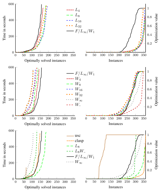
Figure 2: Cactus plots of time and optimization value for runs in Tables 3 and 4. Closeness to the bottom right is better in both cases. For each instance, the best final optimization value reported by a system is mapped to 0 and the worst to 1. From top to bottom, the horizontal pairs of plots concern systems $L_{d}$ using rewriting with depth $d$ networks, systems $W_{k}$ using rewriting with weights on every $k$th layer, and a selection of these systems together with clasp using core-guided optimization (usc) and branch-and-bound (clasp).

In the process of these experiments, additional preliminary screening was performed on various aspects of the benchmark setting. The results are only briefly described here due to lacking significance in the outcomes. For one, a significantly extended timeout of one hour had little impact on the relative standing of the pipelines. Likewise, use of a stratification heuristic for handling weights in clasp when employing core-guided optimization made little difference. Moreover, the combination of rewriting and core-guided optimization performed otherwise similarly to plain core-guided optimization, but resulted in more timeouts.

Further benchmark classes were also screened for an impact due to optimization rewriting. To this end, Steiner Tree, Valves Location, and Video Streaming from the ASP Competitions were considered, but none showed clear signs of improvements to report. These benchmarks are generally large, and have geometric averages 5.7, 5.5, and 4.5 of constraints on a logarithmic scale before rewriting, respectively. On Valves Location, the results were neutral and on the other two, performance was reduced. On Valves Location, the explanation may be in that the optimization statements are minuscule relative to the entire instances, which may reflect their significance as sources of nogoods. On Video Streaming, the performance reduction is minor. On Steiner Tree, the reduction is greater, and the reason may simply be that the size blowup is particularly costly given the exceptionally large size of the instances already before rewriting. In general, an exceptionally large input size for a solvable instance is a sign of the instance being “large but easy” rather than “small but hard”, and it is likely that its difficulty does not stem as heavily from a combinatorial explosion as with smaller instances. This may hinder the usefulness of the proposed optimization rewriting since based on the formal analysis, optimization rewriting yields benefits in cases where the task of optimization presents a clear combinatorial challenge.

In summary, our experiments provide support in favor of different solving pipelines on different benchmark classes. Thus, an ideal portfolio solver incorporating the proposed optimization rewriting techniques and native optimization approaches would surpass either approach standing alone. In particular, our optimization rewriting pipelines improve in several cases over plain clasp as well as clasp with core-guided optimization. Based on the results, we recommend considering optimization rewriting based on depth limited comparator networks as in $L_{d}$ where $d$ is ideally tuned based on the benchmark set at hand or fixed to a modest value such as $d=8$, which yielded robust performance in these experiments. Limiting network depth limits rewriting size while compromising some of the benefits of rewriting and generally, although not always, this tradeoff is worthwhile. Moreover, due to differences in the result statuses and the $S_{1}$ scores, we hypothesize that the proposed optimization rewriting techniques are particularly suitable for solving instances all the way to optimality.

5 Related Work

The odd-even merge sort scheme [Batcher (1968)] is a widely used scheme for generating practical and useful sorting networks. Sorting networks have existing applications in, e.g., SAT encodings of pseudo-Boolean constraints [Eén and Sörensson (2006)]. These SAT encodings simulate summation in a binary system with digits encoded in a unary number system. The number of sorting networks used is proportional to the maximum bit width of the weights in the pseudo-Boolean constraint being encoded. Moreover, the number of inputs to each sorting network is proportional to the number of inputs to the constraint. We have carried these techniques over to ASP in our previous work on the normalization of cardinality rules [Bomanson and Janhunen (2013)] and weight rules [Bomanson et al. (2014)]. For weight rules, a set of structurally shared sorters is used to compensate for a bit-width induced blowup factor originating from sorting network based SAT encodings [Eén and Sörensson (2006)]. This line of research led to optimization rewriting [Bomanson et al. (2016)], which is also the focus of Section 4. In contrast to normalization, where special constraints are compiled away altogether, the goal of rewriting is more relaxed and concerns the reformulation of optimization statements received as input with the help of additional atoms and rules. Section 4 furnishes the weight propagation concept introduced in this paper to provide a novel optimization rewriting technique. The technique is distinguished by the fact that it always requires only a single comparator network regardless of the bit width of input weights. Moreover, the network needs to be only a comparator network, as opposed to a sorting network. These properties make it easier to find a network that meets any desired depth and size parameters, which can be chosen to maximize performance on a given class of problems.

In the context of optimization, sorting networks have also been used to express sets of mutually similar cardinality constraints generated during solving by the (unsatisfiable) core-guided Maximum Satisfiability (MaxSAT) solver MSCG [Morgado et al. (2014)]. MaxSAT is closely related to ASP optimization, witnessed by the fact that the mentioned solver builds on the algorithm OLL originally devised for ASP optimization [Andres et al. (2012)] in the ASP solver clasp. Core-guided optimization methods such as these start from the unfeasible region of the search space, solving progressively relaxed, unsatisfiable subproblems until a solution is found. In this solving process, reasons for unsatisfiability are characterized by so-called unsatisfiable cores that form the basis of analysis in the OLL algorithm, which yields cardinality constraints used to guide the relaxation steps. In the more traditional, model-guided optimization strategy, such as branch-and-bound, search begins from the feasible region of the search space, as models of successively improved value are sought until no improvement is possible [Alviano et al. (2015)]. In experimental evaluations presented in Section 4.4, optimization rewriting and model-guided optimization are compared against core-guided optimization, and the techniques are found to excel at different benchmarks. However, in contrast to core-guided methods, optimization rewriting works in principle with any solving approach by virtue of being a preprocessing technique. This includes model-guided optimization, to which it contributes the benefits of comparator network encodings.

Another recent development [Saikko et al. (2018)] in ASP optimization is to isolate all arithmetic reasoning into a separate implicit hitting set (IHS) problem [Moreno-Centeno and Karp (2013)]. The approach stems from MaxSAT [Davies and Bacchus (2011)], and can be seen as a variation of core-guided optimization where the relaxation steps are performed differently in order to cope better with non-unit weights. Namely, each core is encoded together with the optimization criteria in an IHS problem that can be solved via integer linear programming (ILP). The solution to the IHS problem is used in relaxing the problem in a way that requires no added rules. The use of an ILP solver for this task results in a hybrid approach for ASP optimization that alternates between ASP decision solving for core extraction and IHS solving via ILP for problem relaxation [Saikko et al. (2018)]. The specific avoidance of new rules and atoms, and the outsourcing of arithmetic computations to an external solver are in stark contrast with this work and indicate that the approach seeks performance benefits via a highly orthogonal manner. Indeed, the approach does not empower the ASP computation with the potential benefits of new auxiliary atoms discussed in Section 4. Moreover, a combination of the approaches is possible and may prove fruitful, but such a study is left out of the scope of this work.

There is existing work on formally analyzing abstract solvers for SAT and ASP. The analysis in Section 4.2 is distinguished from existing work that we are aware of in that it shows an exponential improvement in propagator based solving of optimization problems in answer set programming. Regarding the related work, Anger et al. (?) demonstrated that simple program transformations that add structure to an answer set program can exponentially reduce the search space explored by a state-of-the-art answer set solver of the time. The added structure was in the form of new intermediate atoms and rules used to explicitly express rule bodies. A formal proof system was provided by Gebser and Schaub (?) and used to prove exponentially different best-case computation lengths between different ASP algorithms. The proof system was a form of tableaux calculi. It was extended by Järvisalo and Oikarinen (?) to form Extended ASP Tableaux, which further defines an extension rule based on the addition of redundant structure in the form of added rules. This addition of redundant structure was proven to enable polynomial length proofs on a family of normal logic programs on which proofs in the original proof system were of exponential length at minimum. In the field of SAT and SMT, an abstract framework was put forth by Järvisalo and Oikarinen (?) for describing standard search procedures for SAT. In the framework, graphs are used to capture the behavior of solving algorithms. In the graphs, nodes represent solver states and directed edges represent various actions that the algorithms may perform to move between states. The graphs facilitate formally precise description of algorithms as well as analysis of their properties. Based on this framework for SAT and SMT, a similar framework was developed for describing, analyzing and comparing various ASP solving algorithms [Lierler (2011)]. More recently, a framework was developed for integrating multiple reasoning formalisms, such as SAT and ASP, together as equal standing components [Lierler and Truszczynski (2016)]. The framework is able to incorporate the semantics of both propositional theories and logic programs, and moreover SMT can be translated into it.

6 Conclusion

In this paper, we present a novel technique for rewriting pseudo-Boolean expressions deployed as objective functions in ASP and other constraint-based paradigms. The technique is based on the novel idea of connecting an encoding of a comparator network to the literals of an objective function and redistributing the coefficients of the objective function systematically over the structure of the network as weights. When translated into a target formalism, such as ASP, auxiliary atoms used to express the structure of the network offer the underlying back-end solver additional branching points and concepts to learn about. In this paper, we formally analyzed and experimentally evaluated the idea in the context of ASP. As part of this, we provide a formal analysis that highlights an exponential separation in solving performance on an example family of answer set programs. We implemented the approach in a tool called pbtranslate, which we evaluated in computational experiments. In the experiments, we obtained positive experimental results using pbtranslate for rewriting optimization statements and clasp (v. 3.3.3) as the back-end ASP solver. We found several benchmark problems where the search for an optimal answer set is significantly accelerated using designs based on sorting networks. This holds in comparison to both branch-and-bound and core-guided optimization strategies of clasp. Although rewritten optimization statements have an increased size, the introduction of useful auxiliary variables and the redistribution of weights more than compensates for this cost on these benchmark problems. The idea is moreover completely general and we anticipate further applications of this technique in neighboring paradigms in addition to ASP. As regards future work, we believe it is worthwhile to consider similar techniques using more general types of networks, such as permutation networks [Waksman (1968)].

References

- Abío et al. (2012) Abío, I., Nieuwenhuis, R., Oliveras, A., Rodríguez-Carbonell, E., and Mayer-Eichberger, V. 2012. A new look at bdds for pseudo-boolean constraints. Journal of Artificial Intelligence Research 45, 443–480.
- Abío et al. (2013) Abío, I., Nieuwenhuis, R., Oliveras, A., Rodríguez-Carbonell, E., and Stuckey, P. J. 2013. To encode or to propagate? The best choice for each constraint in SAT. In Proceedings of CP 2013, C. Schulte, Ed. LNCS, vol. 8124. Springer, 97–106.
- Alviano et al. (2015) Alviano, M., Dodaro, C., Leone, N., and Ricca, F. 2015. Advances in WASP. In Proceedings of LPNMR 2015, F. Calimeri, G. Ianni, and M. Truszczynski, Eds. LNCS, vol. 9345. Springer, 40–54.
- Alviano et al. (2015) Alviano, M., Dodaro, C., Marques-Silva, J., and Ricca, F. 2015. Optimum stable model search: algorithms and implementation. Journal of Logic and Computation.
- Andres et al. (2012) Andres, B., Kaufmann, B., Matheis, O., and Schaub, T. 2012. Unsatisfiability-based optimization in clasp. See Dovier and Santos Costa (2012), 212–221.
- Anger et al. (2006) Anger, C., Gebser, M., Janhunen, T., and Schaub, T. 2006. What’s a head without a body? In Proceedings of ECAI 2006. IOS Press, 769–770.
- Apt et al. (1987) Apt, K., Blair, H., and Walker, A. 1987. Towards a theory of declarative knowledge. In Foundations of Deductive Databases and Logic Programming, J. Minker, Ed. Morgan Kaufmann Publishers, Chapter 2, 89–148.
- Balduccini and Janhunen (2017) Balduccini, M. and Janhunen, T., Eds. 2017. Proceedings of LPNMR 2017. LNCS, vol. 10377. Springer.
- Banbara et al. (2013) Banbara, M., Soh, T., Tamura, N., Inoue, K., and Schaub, T. 2013. Answer set programming as a modeling language for course timetabling. Theory and Practice of Logic Programming 13, 4-5, 783–798.
- Batcher (1968) Batcher, K. E. 1968. Sorting networks and their applications. In AFIPS Spring joint computer conference. ACM, Thomson Book Company, 307–314.
- Bomanson (2017) Bomanson, J. 2017. lp2normal - A normalization tool for extended logic programs. See Balduccini and Janhunen (2017), 222–228.
- Bomanson et al. (2014) Bomanson, J., Gebser, M., and Janhunen, T. 2014. Improving the normalization of weight rules in answer set programs. In Proceedings of JELIA 2014. LNCS, vol. 8761. Springer, 166–180.
- Bomanson et al. (2016) Bomanson, J., Gebser, M., and Janhunen, T. 2016. Rewriting optimization statements in answer-set programs. In Technical Communications of ICLP 2016. OASIcs, vol. 52. Schloss Dagstuhl–Leibniz-Zentrum für Informatik, 5:1–5:15. Article 5.
- Bomanson and Janhunen (2013) Bomanson, J. and Janhunen, T. 2013. Normalizing cardinality rules using merging and sorting constructions. In Proceedings of LPNMR 2013. LNCS, vol. 8148. Springer, 187–199.
- Bonutti et al. (2012) Bonutti, A., De Cesco, F., Di Gaspero, L., and Schaerf, A. 2012. Benchmarking curriculum-based course timetabling: Formulations, data formats, instances, validation, visualization, and results. Annals of Operations Research 194, 1, 59–70.
- Brewka et al. (2011) Brewka, G., Eiter, T., and Truszczyński, M. 2011. Answer set programming at a glance. Communications of the ACM 54, 12, 92–103.
- Calimeri et al. (2013) Calimeri, F., Faber, W., Gebser, M., Ianni, G., Kaminski, R., Krennwallner, T., Leone, N., Ricca, F., and Schaub, T. 2013. ASP-Core-2: 4th ASP Competition official input language format. Available as http://www.mat.unical.it/aspcomp2013/files/ASP-CORE-2.01c.pdf.
- Calimeri et al. (2015) Calimeri, F., Ianni, G., and Truszczynski, M., Eds. 2015. Proceedings of LPNMR 2015. LNCS, vol. 9345. Springer.
- Clark (1978) Clark, K. 1978. Negation as failure. In Logic and Data Bases. Plenum Press, 293–322.
- Cussens (2011) Cussens, J. 2011. Bayesian network learning with cutting planes. In Proceedings of UAI 2011, F. Cozman and A. Pfeffer, Eds. AUAI Press, 153–160.
- Davies and Bacchus (2011) Davies, J. and Bacchus, F. 2011. Solving MAXSAT by solving a sequence of simpler SAT instances. In Proceedings of CP 2011, J. H. Lee, Ed. LNCS, vol. 6876. Springer, 225–239.
- Denecker et al. (2009) Denecker, M., Vennekens, J., Bond, S., Gebser, M., and Truszczyński, M. 2009. The second answer set programming competition. In Proceedings of LPNMR 2009, E. Erdem, F. Lin, and T. Schaub, Eds. LNAI, vol. 5753. Springer, 637–654.
- Dovier and Santos Costa (2012) Dovier, A. and Santos Costa, V., Eds. 2012. Technical Communications of ICLP 2012. Vol. 17. Leibniz International Proceedings in Informatics (LIPIcs).
- Drescher and Walsh (2012) Drescher, C. and Walsh, T. 2012. Answer set solving with lazy nogood generation. See Dovier and Santos Costa (2012), 188–200.
- Eén and Sörensson (2006) Eén, N. and Sörensson, N. 2006. Translating Pseudo-Boolean constraints into SAT. Journal on Satisfiability, Boolean Modeling and Computation 2, 1–4, 1–26.
- Gebser et al. (2015) Gebser, M., Kaminski, R., Kaufmann, B., Romero, J., and Schaub, T. 2015. Progress in clasp series 3. See Calimeri et al. (2015), 368–383.
- Gebser et al. (2012) Gebser, M., Kaufmann, B., and Schaub, T. 2012. Conflict-driven answer set solving: From theory to practice. Artificial Intelligence 187, 52–89.
- Gebser et al. (2015) Gebser, M., Maratea, M., and Ricca, F. 2015. The design of the sixth answer set programming competition. See Calimeri et al. (2015), 531–544.
- Gebser et al. (2017) Gebser, M., Maratea, M., and Ricca, F. 2017. The design of the seventh answer set programming competition. See Balduccini and Janhunen (2017), 3–9.
- Gebser and Schaub (2013) Gebser, M. and Schaub, T. 2013. Tableau calculi for logic programs under answer set semantics. ACM Transactions on Computational Logic 14, 2, 15:1–15:40.
- Jaakkola et al. (2010) Jaakkola, T., Sontag, D., Globerson, A., and Meila, M. 2010. Learning Bayesian network structure using LP relaxations. In Proceedings of AISTATS 2010. JMLR Proceedings, vol. 9. JMLR, 358–365.
- Janhunen et al. (2017) Janhunen, T., Gebser, M., Rintanen, J., Nyman, H., Pensar, J., and Corander, J. 2017. Learning discrete decomposable graphical models via constraint optimization. Statistics and Computing 27, 1, 115–130.
- Janhunen and Niemelä (2016) Janhunen, T. and Niemelä, I. 2016. The answer set programming paradigm. AI Magazine 37, 3, 13–24.
- Järvisalo and Oikarinen (2008) Järvisalo, M. and Oikarinen, E. 2008. Extended ASP tableaux and rule redundancy in normal logic programs. Theory and Practice of Logic Programming 8, 5-6, 691–716.
- Lierler (2011) Lierler, Y. 2011. Abstract answer set solvers with backjumping and learning. Theory and Practice of Logic Programming 11, 2-3, 135–169.
- Lierler and Truszczynski (2016) Lierler, Y. and Truszczynski, M. 2016. On abstract modular inference systems and solvers. Artificial Intelligence 236, 65–89.
- Lifschitz and Razborov (2006) Lifschitz, V. and Razborov, A. A. 2006. Why are there so many loop formulas? ACM Transactions on Computational Logic 7, 2, 261–268.
- Lifschitz and Turner (1994) Lifschitz, V. and Turner, H. 1994. Splitting a logic program. In Proceedings of ICLP 1994. MIT Press, 23–37.
- Maratea et al. (2015) Maratea, M., Pulina, L., and Ricca, F. 2015. Multi-level algorithm selection for ASP. See Calimeri et al. (2015), 439–445.
- MaxSAT-Comp (2014) MaxSAT-Comp. 2014. Ninth Max-SAT evaluation. Available as http://www.maxsat.udl.cat/14/.
- Moreno-Centeno and Karp (2013) Moreno-Centeno, E. and Karp, R. M. 2013. The implicit hitting set approach to solve combinatorial optimization problems with an application to multigenome alignment. Operations Research 61, 2, 453–468.
- Morgado et al. (2014) Morgado, A., Dodaro, C., and Marques-Silva, J. 2014. Core-guided maxsat with soft cardinality constraints. In Proceedings of CP 2014, B. O’Sullivan, Ed. LNCS, vol. 8656. Springer, 564–573.
- Nieuwenhuis et al. (2006) Nieuwenhuis, R., Oliveras, A., and Tinelli, C. 2006. Solving SAT and SAT modulo theories: From an abstract Davis–Putnam–Logemann–Loveland procedure to DPLL(T). Journal of the ACM 53, 6, 937–977.
- Saikko et al. (2018) Saikko, P., Dodaro, C., Alviano, M., and Järvisalo, M. 2018. A hybrid approach to optimization in answer set programming. In Proceedings of KR 2018, M. Thielscher, F. Toni, and F. Wolter, Eds. AAAI Press, 32–41.
- Waksman (1968) Waksman, A. 1968. A permutation network. Journal of the ACM 15, 1, 159–163.
- Zhou and Kjellerstrand (2016) Zhou, N. and Kjellerstrand, H. 2016. The picat-sat compiler. In Proceedings of PADL 2016, M. Gavanelli and J. H. Reppy, Eds. LNCS, vol. 9585. Springer, 48–62.