Probing Crust Meltdown in Inspiraling Binary Neutron Stars

Abstract

Thanks to recent measurements of tidal deformability and radius, the nuclear equation of state and structure of neutron stars are now better understood. Here, we show that through resonant tidal excitations in a binary inspiral, the neutron crust generically undergoes elastic-to-plastic transition, which leads to crust heating and eventually meltdown. This process could induce $\sim\mathcal{O}(0.1)$ phase shift in the gravitational waveform. Detecting the timing and induced phase shift of this crust meltdown will shed light on the crust structure, such as the core-crust transition density, which previous measurements are insensitive to. A direct search using GW170817 data has not found this signal, possibly due to limited signal-to-noise ratio. We predict that such signal may be observable with Advanced LIGO Plus and more likely with third-generation gravitational-wave detectors such as the Einstein Telescope and Cosmic Explorer.

Introduction. Inspiraling neutron stars deform under mutual tidal interactions. In the adiabatic limit, the star’s induced quadrupole moment is directly proportional to the tidal gravitational field, with the proportionality constant given by the tidal Love number. Deformed neutron stars orbit each other differently from black holes with the same masses, and the phase difference can be used to measure the tidal Love number Flanagan and Hinderer (2008), as shown in the analysis of GW170817 Abbott et al. (2018). Together with neutron star radius measurements Miller et al. (2019), maximum mass estimates Rezzolla et al. (2018) and possibly post-merger electromagnetic signals Radice et al. (2018), the star’s equation of state (EoS) is now better constrained.

In addition to adiabatic tides, tidal interaction can excite internal modes of neutron stars as the binary sweeps through the inspiral frequency range. The pressure (p-) and fundamental (f-)modes Kokkotas and Schmidt (1999) will not be fully excited as their frequencies are generally higher than the inspiral frequency, although it has been suggested that early excitation of f-modes may be observed in the late inspiral stage Pratten et al. (2019). Gravity modes may be fully excited, but their couplings to tidal gravitational fields are so small that the induced phase shifts are $\mathcal{O}(10^{-3})$ or smaller Lai (1994); Yu and Weinberg (2017). Resonance of rotational modes has also been investigated assuming a rotational frequency of a few $\times 10^{2}$ Hz Ho and Lai (1999); Lai and Wu (2006); Flanagan and Racine (2007a); Poisson (2020), whereas the fastest rotating pulsar known in a binary neutron star system has a frequency of $\sim 60$ Hz Burgay et al. (2003); Andrews and Mandel (2019).

The interface (i-)modes McDermott et al. (1985, 1988), excited at the interface of the fluid core and solid crust, have frequencies around several tens to a few hundred Hertz, depending on the star’s equation of state and prescription of the crust. The resonance of i-modes was proposed to explain precursors of short gamma-ray bursts due to possible crust failures Tsang et al. (2012). We observe that through excitation of i-modes, the crustal material actually reaches its elastic limit well before the mode resonance. After reaching this threshold the crust undergoes an elastic-to-plastic transition and the tidal driving starts to heat up the crust. The whole process ends with the meltdown of the crust in tens of cycles.

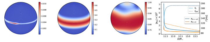
Figure 1: Left three panels are the heat maps $e_{i}/e_{\rm melt}$ of the neutron star crust (within a $1.3M_{\odot}+1.3M_{\odot}$ binary) at binary separations $D=12.0/11.6/11.4\ R_{\star}$, respectively. In the rightmost panel, dashed lines denote the evolution of the i-mode frequency $f_{0}$ and the gravitational wave (GW) frequency $f_{\rm GW}$, and solid lines denote the evolution of mode amplitude $a_{m}$ with $m=\pm 2,0$.

Crust heating up and melting down. The outer part of the crust is commonly described by a Coulomb lattice with shear modulus $\mu$ Strohmayer et al. (1991). The inner crust may have nonuniform structures associated with the “nuclear pasta” phase Ravenhall et al. (1983); Hashimoto et al. (1984), which is not considered in this study. Simulations of molecular dynamics Chugunov and Horowitz (2010) have shown that the lattice responds elastically under small applied stress; once the induced strain exceeds the breaking strain ($\epsilon_{b}\sim 0.1$), plastic deformation starts to develop. Assuming an applied stress $\sigma$, the plastic deformation rate $\dot{\epsilon}_{\rm pl}$ is exponentially small if $\sigma<\sigma_{b}=\mu\epsilon_{b}$, and becomes exponentially large if $\sigma>\sigma_{b}$. Mathematically, it is well approximated by Chugunov and Horowitz (2010)

$$\dot{\epsilon}_{\rm pl}=\frac{n_{i}Z^{2}e^{2}}{a}\frac{\omega_{\rm p}}{\mu\bar{N}\Gamma}e^{(-18.5\bar{\sigma}_{b}+\bar{\sigma}\bar{N})\Gamma}\ ,$$ (1)

where the dot denotes a time derivative, $\omega_{\rm p}$ is the plasma frequency, $\bar{N}=500/(\Gamma-149)+18.5$, $\bar{\sigma}=\sigma/(n_{i}Z^{2}e^{2}/a)$ and $\Gamma=Z^{2}e^{2}/aT$ is the melting parameter with $e$ the electron charge, $Ze$ the total charge per ion, $a$ the lattice spacing, $n_{i}$ the ion density and $T$ the temperature. The elastic part of the strain $\epsilon_{\rm el}$ satisfies $\sigma=\mu\epsilon_{\rm el}$ and the total strain is simply $\epsilon=\epsilon_{\rm el}+\epsilon_{\rm pl}$.

With the plastic deformation, mode energy dissipates into thermal energy, heating up the crust with a rate Thompson et al. (2017)

$$n_{i}\dot{e}_{i}=\sigma\dot{\epsilon}_{\rm pl}(\sigma,T)\ ,$$ (2)

where $n_{i}$ is the ion number density, $e_{i}$ is the thermal energy per ion, and $de_{i}=c_{V}dT$ with $c_{V}$ the specific heat capacity for $T<T_{\rm melt}$ Chabrier (1993). Once the melting temperature $T_{\rm melt}$ is reached, the crustal material still needs an extra amount of latent heat ($\sim kT_{\rm melt}$ per ion) to be melted Shapiro and Teukolsky (1983). As a result, the total energy per ion needed to melt the crust from its initial cold state is roughly $e_{\rm melt}=\int_{0}^{T_{\rm melt}}c_{V}dT+kT_{\rm melt}$. In this work we have ignored contributions from dripped neutrons as their specific heat may be suppressed by superfluidity.

Mode Analysis. In the linear approximation, the stellar response to the tidal force is specified by the Lagrangian displacement $\bm{\xi}(\bm{r},t)$ of a fluid element from its equilibrium position. The displacement can be decomposed into eigenmodes, $\bm{\xi}(\bm{r},t)=\sum_{\alpha}a_{\alpha}(t)\bm{\xi}_{\alpha}(\bm{r})$, where $\alpha$ denotes the quantum number of an eigenmode. In the context of this paper, we only consider i-modes driven by the leading quadrupole term of the tidal force, so that $\bm{\xi}_{m}(\bm{r})=[U(r)\hat{r}+rV(r)\nabla]Y_{2m}(\theta,\phi)$, where $Y_{2m}(\theta,\phi)$ is the $l=2$ spherical harmonic. The displacement behavior is governed by the linear pulsation equation McDermott et al. (1985, 1988)

$$[\mathcal{L}(r;\mu)-\omega_{0}^{2}]\bm{\xi}_{m}=0\ ,$$ (3)

with $\mathcal{L}$ being an operator specifying the restoring force inside the star (see Supplemental Material Sup for the explicit expression).

For the example star with $M_{\star}=1.3M_{\odot},R_{\star}=11.7$ km assuming SLy4 EoS Douchin and Haensel (2001); Read et al. (2009) and a core-crust baryon transition density $n_{\rm b,cc}=0.065\ {\rm fm}^{-3}$, we obtain an i-mode frequency $f_{0}=\omega_{0}/2\pi=190$ Hz McDermott et al. (1988); Tsang et al. (2012) and the tidal coupling coefficient (a measure quantifying the overlap between the waveform and the tidal field)

$$Q=\frac{1}{M_{\star}R_{\star}^{2}}\int d^{3}x\rho\ \bm{\xi_{m}^{*}}\cdot\nabla[r^{2}Y_{2m}(\theta,\phi)]=0.018,$$ (4)

with the normalization $\braket{\bm{\xi}_{m}}{\bm{\xi}_{m^{\prime}}}:=\int d^{3}x\rho\ \bm{\xi_{m}}\cdot\bm{\xi}^{*}_{m^{\prime}}=\delta_{mm^{\prime}}M_{\star}R_{\star}^{2}$, where $\rho$ is the mass density .

The evolution of the mode amplitude $a_{m}(t)$ is governed by Lai (1994)

$$\ddot{a}_{m}+\gamma(t)\dot{a}_{m}+\omega_{0}^{2}(t)a_{m}=\frac{GM^{\prime}W_{2m}Q}{D^{3}}e^{-im\Phi(t)}\ ,$$ (5)

where the right-hand side is the leading quadrupole term of the tidal driving force with $M^{\prime}=qM_{\star}$ the companion star mass, $D$ the binary seperation, $\Phi(t)$ the orbital phase and $W_{2m}$ is a coefficient of $\mathcal{O}(1)$ (see Eq. (2.4) in Ref. Lai (1994)). On the left-hand side, $\gamma(t)\dot{a}_{m}$ is a damping term capturing the plastic deformation induced dissipation with $\gamma(t)$ defined as the ratio between the mode energy dissipation rate and two times the mode kinetic energy, i.e.,

$$\gamma(t)=\frac{\int_{\rm crust}n_{i}\dot{e}_{i}\ d^{3}x}{M_{\star}R_{\star}^{2}\sum_{m}|\dot{a}_{m}|^{2}}\ ,$$ (6)

where the numerator is the crust heating rate (which is equal to the mode energy dissipation rate), and the mode kinetic energy is $\frac{1}{2}\int d^{3}x\rho\bm{\dot{\xi}}(\bm{r},t)\cdot\bm{\dot{\xi}}^{*}(\bm{r},t)=\frac{1}{2}M_{\star}R_{\star}^{2}\sum_{m}|\dot{a}_{m}|^{2}$. The mode frequency $\omega_{0}(t)$ to leading order is determined by (see Eq. (3))

$$\omega_{0}^{2}(t)=\frac{\braket{\bm{\xi}_{m}}{\mathcal{L}(r;\mu_{\rm avg})\bm{\xi}_{m}}}{\braket{\bm{\xi}_{m}}{\bm{\xi}_{m}}}\ ,$$ (7)

where $\mu_{\rm avg}$ is the average shear modulus which decreases as the crust is heated and we find the mode frequency is roughtly proportional to the square root of the average shear modulus Passamonti and Andersson (2012).

Given the mode amplitude $a_{m}(t)$, it is straightforward to calculate the fluid element displacement $\bm{\xi}(\bm{r},t)=\sum_{m}a_{m}(t)\bm{\xi}_{m}(\bm{r})$ and the corresponding strain $\epsilon_{\rm el}$. From equation (1), the plastic deformation rate $\dot{\epsilon}_{\rm pl}$ has an exponential dependence on the local strain $\epsilon_{\rm el}$ for $\epsilon_{\rm el}\gtrsim 0.1$, so does the energy dissipation rate $\sigma\dot{\epsilon}_{\rm pl}$. Physically, the dissipated energy comes from the local elastic energy, therefore the energy dissipation rate cannot exceed its replenishment rate $\frac{\mathcal{A}}{2}\mu\epsilon_{\rm el}^{2}f_{\rm GW}$, where $f_{\rm GW}$ is the frequency of both the tidal force and the GW emission and $\mathcal{A}$ is a coefficient of $\mathcal{O}(1)$. Here we take $\mathcal{A}=2$ as an example. As for the initial condition, we choose $T_{i}=0.02T_{\rm melt}$, where $T_{\rm melt}\sim 1$ MeV is the melting temperature of the ion crystal at the crust base Strohmayer et al. (1991). Using the 4th-order Runge-Kutta scheme, we evolve Equations (1, 2, 5) on the two-dimensional surface of the crust base, i.e., we only trace the thermal evolution of the crust base considering its dominant role in the crust heat capacity.

As the neutron star binary spirals inward, the tidal field increases and so does the i-mode amplitude $a_{m=0,\pm 2}$, as shown in Fig. 1. At a certain binary separation (with corresponding gravitational wave frequency $f_{\rm GW,melt}<f_{0}$), part of the crust reaches the yield limit $\epsilon_{b}$ due to the i-mode excitation and plastic deformation starts. Heating first takes place at the equator where the strain maximizes. As the crust heats up, it softens so that i-mode frequency $f_{0}$ decreases and the mode amplitude $a_{m}$ increases. As a result, the crust yields on larger and larger areas, extending from the equator to the poles, and finally the whole crust is melted. The crust melting takes about $20$ orbit periods and a total amount of energy $E_{\rm melt}\simeq 1.1\times 10^{47}$ ergs. Notice that this mode treatment is approximate once the plastic motion turns on, where a more accurate description requires 3-dimensional dynamical modeling of crustal motions. A 2-dimensional consistent evolution was implemented in Thompson et al. (2017) to reveal yield patterns of magnetar crust under strong magnetic stress.

Waveform signature. After the melting process, part of the binary orbital energy is converted to the mode and thermal energy resulting in a phase shift of the gravitational waveform. Similar to the discussion in Lai (1994); Flanagan and Racine (2007b); Yu and Weinberg (2017) for mode resonances, for the binary neutron star waveform $h(f)=A(f)e^{i\Psi(f)}$, its phase is modified as

$$\delta\Psi(f) =\sum_{i=1,2}\delta\phi_{i}\left(1-\frac{f}{f_{i}}\right)\Theta(f-f_{i})\,$$

$$\approx\delta\phi_{a}\left(1-\frac{f}{f_{a}}\right)\Theta(f-f_{a})$$ (8)

where $\Theta$ is the Heaviside function and $f_{i}$ is the melting frequency of each star. Therefore the search and forecast presented below for crust melting apply equally for generic mode resonances, and we will use ‘mode resonance signature’ and ‘crust melting signature’ interchangeably. The melting process decreases the coalescence phase by $\delta\phi_{i}$ and the coalescence time by $\delta\phi_{i}/2\pi f_{i}$. In the second line we introduced $\delta\phi_{a}=\sum_{i}\delta\phi_{i}$ and $\delta\phi_{a}/f_{a}=\sum_{i}\delta\phi_{i}/f_{i}$ to reduce the number of extra parameters in this model, which simplifies the parameter estimation process. Notice that if energy transfers from the orbit to the mode (or heat in this case) during resonance, $\delta\phi$ is positive; if energy transfers from the mode to the orbit, as expected in some of the r-mode resonances Flanagan and Racine (2007a), $\delta\phi$ is negative.

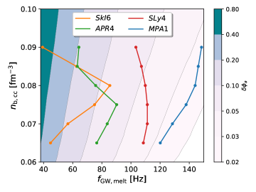
Figure 2: The crust melting induced phase change $\delta\phi_{a}$ in GWs of a BNS merger with each star of $M_{\star}=1.3M_{\odot}$ and $R_{\star}=12.5/11.3/11.7/12.7$ km for the EoS SkI6/APR4/SLy4/MPA1, respectively, which are not ruled out by the LIGO tidal measurement with GW170817. Note that the core-crust transition density $n_{\rm b,cc}$ is subject to a large uncertainty in each EoS instead of being an accurately predicted value, so we take the transition density as a free parameter.

For each neutron star, $\delta\phi$ depends on its mass $M_{\star}$, the mass ratio of the companion $q$ (with the companion mass being $qM_{\star}$), the melting energy $E_{\rm melt}$ and the melting frequency $f_{\rm GW,melt}$ as follows Lai (1994)

$$\delta\phi=\frac{2\omega_{\rm orb}E_{\rm melt}}{P_{\rm GW}}\simeq\frac{0.1}{q^{2}}\left(\frac{1+q}{2}\right)^{2/3}\ E_{47}M_{1.3}^{-10/3}f_{70}^{-7/3}\ ,$$ (9)

where $\omega_{\rm orb}=\pi f_{\rm GW,melt}$ is the orbital angular frequency, $P_{\rm GW}$ is the energy loss rate due to GW emission, and $E_{47}=E_{\rm melt}/10^{47}{\rm ergs},M_{1.3}=M_{\star}/1.3M_{\odot},f_{70}=f_{\rm GW,melt}/70{\rm Hz}$. From Equation (9), we immediately see that the phase shift increases if the melting process happens earlier (lower $f_{\rm GW,melt}$) in the inspiral phase. In Fig. 2, we show the total phase change $\delta\phi_{a}$ for an equal-mass binary neutron star (BNS) merger with $M_{\star}=1.3M_{\odot}$, where $\delta\phi_{a}$ varies from $0.03$ to $0.6$ depending on the star’s EoS and the core-crust transition baryon density $n_{\rm b,cc}$. The melting energy increases substantially with increasing $n_{\rm b,cc}$ (commonly assumed to be within $0.06-0.1\ {\rm fm}^{-3}$ Horowitz and Piekarewicz (2001); Xu et al. (2009); Moustakidis et al. (2010)), whereas the i-mode frequency and the associated melting frequency are non-monotonic functions of $n_{\rm b,cc}$. We also note that since the mode calculation presented here is Newtonian with the Cowling approximation Cowling (1941), the fully relativistic mode frequencies may be different (for examples, the frequencies of p- and f-modes are smaller with the metric perturbation included Yoshida and Kojima (1997); Chirenti et al. (2015)). If there are also more unpaired neutrons present within the star, as suggested by the cooling measurement in Brown et al. (2018), the melting energy may be significantly boosted and the internal mode spectrum may be modified as well. Therefore the search of mode resonance signatures may also help probe the superfluid composition of neutron stars. The effects of nuclear pastas on the melting energy budget and the mode frequency determination also need to be better understood. Nevertheless, the measurement of $f_{a}$ and $\delta\phi_{a}$ will convey useful information about the core-crust transition density and the star’s EoS around that density.

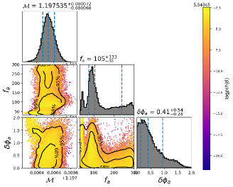
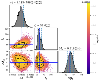
Figure 3: Posterior distribution of chirp mass $\mathcal{M}$, phase shift $\delta\phi_{a}$ and melting frequency $f_{a}$ obtained with PyCBC, where the prior for $f_{a}$ is set to be $[30,300]$Hz and $[0,2]$ for $\delta\phi_{a}$. Left Plot: the search using data from GW170817. Right Plot: a search obtained assuming LIGO A+ sensitivity and an mode resonance injection at $f_{a}=60$Hz and $\delta\phi_{a}=0.3$.

Search with GW170817. We now present the first search for mode resonance effects (including crust melting) in binary neutron star systems with data from GW170817 with Equation (Probing Crust Meltdown in Inspiraling Binary Neutron Stars) implemented. A similar search for tidal-p-g instability is discussed in Abbott et al. (2019) using different $\delta\Psi(f)$. The Markov-Chain Monte Carlo (MCMC) parameter estimation is performed with PyCBC Biwer et al. (2019), for which we assume the source distance and sky location are known as the electromagnetic counterpart of this source has been identified Abbott et al. (2017). We use the TaylorF2 waveform Buonanno et al. (2009) as the background binary neutron waveform. We present the posterior distributions of chirp mass $\mathcal{M}$, $\delta\phi_{a}$ and $f_{a}$ in Fig. 3. The marginal distribution of $\phi_{a}$ indicates that there is no evidence for mode resonance in GW170817, as $\delta\phi_{a}<1.5$ at $95\%$ confidence level. A similar conclusion can be drawn from a Bayesian model comparison framework. We denote $\mathcal{H}_{a}$ as the hypothesis with mode resonance and $\mathcal{H}_{0}$ as the one without, the Bayes factor can be defined as

$$\mathcal{B}^{a}_{0}=\frac{P({\rm GW170817}|\mathcal{H}_{a})}{P({\rm GW170817}|\mathcal{H}_{0})}$$ (10)

which measures the relative probability of these two hypotheses. We have computed the Bayes factor using both the method of thermodynamic integration Lartillot and Philippe (2006) and the Savage-Dickey Density Ratio method Dickey (1971), which both suggest consistent values of $\log\mathcal{B}^{a}_{0}$ in the range of $[-0.6,-0.3]$. This means that these two hypotheses are essentially indistinguishable with this set of gravitational wave data Kass and Raftery (1995).

It is natural to expect observations with higher signal-to-noise ratios as the sensitivity of gravitational wave detectors improves. In the mid-2020s the upgrade of Advanced LIGO, LIGO A+, is expected to start its constrcution . Assuming LIGO A+ design sensitivity for all three detectors at Hanford/Livingston/India, and Advanced Virgo with its full sensitivity, we may observe GW170817-like events with signal-to-noise ratios beyond 100. In the right panel of Fig. 3, we present a sample search with an injected signal with $\delta\phi_{a}=0.3,f_{a}=60$ Hz (for a GW170817-type system with star masses $m_{1}=1.47M_{\odot},m_{2}=1.28M_{\odot}$, tidal Love numbers $\Lambda_{1}=210.6,\Lambda_{2}=525.6$, zero star spins and nearly face-on orientation with inclination angle $\iota=0.2$ rad) into simulated detector noises consistent with the aforementioned LIGO A+ network sensitivity. We find the mock signal will be detected with SNR$=197$ and a MCMC analysis of the mock data successfully recovers the injected values of $f_{a}$ and $\phi_{a}$ with small uncertainties. So it is possible that we observe the crust melting signature in gravitational waves with LIGO A+.

Stacking different events may also improve detectability, as is the case for subdominant modes in black hole ringdowns Yang et al. (2017). However, we have no prior information on $\delta\phi_{a}$ and $f_{a}$, which are distinct for each binary neutron star system. If we have an underlying or phenomenological model that predicts or characterizes $\delta\phi_{a}$, $f_{a}$ as a function of star mass, core-crust transition density and star compactness (which depends on the EoS), the hyper-parameters in this model may be constrained from different events. Certainly the posterior distribution of the hyper-parameters from different events can be multiple together to form the joint probability distribution. This is something worth to pursue in future studies.

If a mode resonance signature is indeed detected (i.e. preferred over the null hypothesis), it is still necessary to compare to other possible origins, such as tidal-p-g coupling Abbott et al. (2019), dynamical scalarization and vectorization Palenzuela et al. (2014); Annulli et al. (2019), scalar modes associated to certain GR extensions Mendes and Ortiz (2018) and extensions to standard particle physics Huang et al. (2019), that predict different $\delta\Psi(f)$. Since the crust melting is nearly instant (Fig. 1), its impact on the waveform boils down to shifting the coalescence time and the coalescence phase, i.e., $\delta\Psi(f)=\delta\phi_{a}\times(1-f/f_{a})$ with $\delta\phi_{a}$ being a constant. For other processes with continuous orbital energy draining, e.g., the tidal-p-g coupling extending the whole frequency range once the nonlinear instability is turned on, the waveform signature can be formulated in a similar way except with a frequency dependent phase shift $\delta\phi_{a}(f)$ which encodes the details of orbital energy draining. To simulate this, we inject a mode resonance signal ($\delta\phi_{a}=0.3,f_{a}=60$Hz) into detector noise corresponding to the LIGO A+ network, and perform the Bayesian model selection between our model resonance waveform and the tidal-p-g waveform. We find a Bayes factor $\log\mathcal{B}^{a}_{\rm pg}=2.7\pm 0.3$, suggesting that it is also possible to determine the correct model if a positive detection occurs ( see Supplemental Material Sup for more details of the Bayesian analysis). The comparison will be much sharper with third-generation gravitational wave detectors. Similarly for the scalarized neutron stars proposed in scalar tensor theories or other particle physics considerations, there are also effects, such as dipole scalar radiation, that will be effective during the whole frequency range once turned on Huang et al. (2019). We also perform a model selection between the mode resonance and an example model of BNSs with scalar dipole radiation using the same mock data above, and we find the Bayes factor is $\log\mathcal{B}^{a}_{\rm dipole}=11.7\pm 2.2$ (see Supplemental Material Sup ).

Discussion. Resonant tidal excitations in a neutron star binary induce a phase shift $\delta\phi_{a}$ in the gravitational wave signal by melting its crust. In calculating the crust heating rate, we have used the fitting formula $\dot{\epsilon}_{\rm pl}(\sigma)$ [Eq. (1)] which is a result of molecular dynamics simulations Chugunov and Horowitz (2010). If this simulations result does not accurately apply to the NS crust with a breaking strain $\epsilon_{b}$ different from $0.1$, the crust melting frequency $f_{\rm GW,melt}$ will also change. For a smaller breaking strain $\epsilon_{b}=0.05$, we find the melting frequency $f_{\rm GW,melt}$ decreases by $\sim 25\%$ and the phase shift $\delta\phi_{a}$ increases by a factor $\sim 2$. All the predicted phase shifts corresponding to different EoSs are still well consistent with the constraint $\delta\phi_{a}<1.5$ ($95\%$ confidence level) from GW170817. LIGO A+ may already be able to detect such induced phase shifts. A 3rd-generation detector network with Cosmic Explorer Abbott et al. (2017) sensitivity at the LIGO detectors and Einstein Telescope Punturo et al. (2010) sensitivity at the Virgo detector is able to limit $\delta\phi_{a}$ with uncertainty $\sim 0.01$ and $f_{a}$ below 1$\%$. This will not only allow high-confidence detection of the crust melting effect, but also precisely measure crustal and EoS properties as shown in Fig. 2.

We do not expect significant energy release to the neutron star magnetosphere associated with crustal failure, as the magnetic fields ($\sim 10^{12}$G) assumed are too weak to efficiently transfer energy by sending out Alfvén waves. However, if the star is a magnetar with field $\sim 10^{15}$ G, this emission mechanism may excite star magnetospheres and power precursor gamma-ray bursts Thompson et al. (2017); Ackermann et al. (2009); Troja et al. (2010). Interestingly, the recent LIGO observation of a heavy neutron-star binary (GW190425 The LIGO Scientific Collaboration et al. (2020)) may indicate the existence of a fast-merging channel to form binary neutron stars. Such systems may have short-enough lifetime $\sim 10^{4}$ years to allow active magnetars in the binary coalescence stage Yang and Zou (2020).

We thank the referees for giving valuable suggestions. We also thank David Tsang for sharing the code for neutron star mode analysis and Andrea Passamonti for very helpful discussion. Z. P., Z. L. and H. Y. are supported by the Natural Sciences and Engineering Research Council of Canada and in part by Perimeter Institute for Theoretical Physics. Research at Perimeter Institute is supported in part by the Government of Canada through the Department of Innovation, Science and Economic Development Canada and by the Province of Ontario through the Ministry of Colleges and Universities.

Appendix A Pulsation Equations

The motion of a mass element inside a star is governed by the continuity equation, the momentum equation and the Possion equation

$$\frac{\partial\rho}{\partial t}+\nabla\cdot(\rho\bm{v})=0\ ,$$ (11)

$$\frac{\partial\bm{v}}{\partial t}+(\bm{v}\cdot\nabla)\bm{v}=\frac{1}{\rho}\nabla\cdot\bm{\sigma}-\nabla\Phi\ ,$$

$$\nabla^{2}\Phi=4\pi G\rho\ ,$$

where $\bm{\sigma}$ is the stress tensor. In the equilibrium state where $\bm{v}^{(0)}=0$, the stress tensor is simply $\sigma_{ij}^{(0)}=-p\delta_{ij}$ with $p$ being the pressure.

The linear pulsation equations can be derived assuming the Lagrangian displacement $\bm{\xi}(\bm{r},t)=\bm{\xi}(\bm{r})e^{i\omega_{0}t}$ and the potential perturbation $\delta\Phi(\bm{r},t)=\delta\Phi(\bm{r})e^{i\omega_{0}t}$ with $\{\bm{\xi}(\bm{r}),\delta\Phi(\bm{r})\}$ and $\omega_{0}$ being the to-be-determined eigenfunctions and eigenfrequency, respectively. Consequently, we obtain $\bm{v}=\partial\bm{\xi}(\bm{r},t)/\partial t+(\bm{v}^{(0)}\cdot\nabla)\bm{\xi}(\bm{r},t)=\partial\bm{\xi}(\bm{r},t)/\partial t$ and $\sigma_{ij}=\sigma_{ij}^{(0)}+\Gamma_{1}p^{(0)}\epsilon_{kk}\delta_{ij}+2\mu(\epsilon_{ij}-\frac{1}{3}\epsilon_{kk}\delta_{ij})$, where $\Gamma_{1}=(d\ln p/d\ln\rho)_{\rm ad}$ is the adiabatic index, $\epsilon_{ij}=\frac{1}{2}(\xi_{i,j}+\xi_{j,i})$ is the strain tensor and $\mu$ is the shear modulus. Plugging them into Eq. (11), we obtain the linear pulsation equation $[\mathcal{L}(r;\mu)-\omega_{0}^{2}]\bm{\xi}(\bm{r})=0$ with McDermott et al. (1985, 1988)

$$\mathcal{L}(r;\mu)\bm{\xi} =-\nabla\left(\frac{\Gamma_{1}p}{\rho}\nabla\cdot\bm{\xi}\right)-\nabla\left(\frac{1}{\rho}\bm{\xi}\cdot\nabla p\right)+\nabla\delta\Phi$$ (12)

$$+\frac{1}{\rho}\left[\nabla\left(\frac{2}{3}\mu\nabla\cdot\bm{\xi}\right)-\left(\nabla\mu\cdot\nabla\right)\bm{\xi}-\nabla(\bm{\xi}\cdot\nabla\mu)\right]$$

$$+\frac{1}{\rho}\left[(\bm{\xi}\cdot\nabla)\nabla\mu-\mu\left(\nabla^{2}\bm{\xi}+\nabla(\nabla\cdot\bm{\xi})\right)\right]\ ,$$

and the linear Possion equation

$$\nabla^{2}\delta\Phi=-4\pi G(\bm{\xi}\cdot\nabla\rho+\rho\nabla\cdot\bm{\xi})\ .$$ (13)

For spheroidal modes (for example, the i-mode), the displacement vector can be written as a variable-seperation form

$$\bm{\xi}^{r}(\bm{r}) =U(r)Y_{lm}(\theta,\phi)\ ,$$ (14)

$$\bm{\xi}^{\theta}(\bm{r}) =V(r)\frac{\partial Y_{lm}}{\partial\theta}(\theta,\phi)\ ,$$

$$\bm{\xi}^{\phi}(\bm{r}) =\frac{V(r)}{\sin\theta}\frac{\partial Y_{lm}}{\partial\phi}(\theta,\phi)\ ,$$

$$\delta\Phi(\bm{r}) =S(r)Y_{lm}(\theta,\phi)\ .$$

Plugging them into Eqs. (12,13), we obtain the governing equations of $\{U(r),V(r),S(r)\}$ McDermott et al. (1985, 1988)

$$\rho\omega_{0}^{2}U= \rho\frac{d\hat{\chi}}{dr}-\frac{d}{dr}\left(\frac{1}{3}\mu\hat{\alpha}\right)+\frac{d\mu}{dr}\left(\hat{\alpha}-2\frac{dU}{dr}\right)$$ (15)

$$-\mu\left[\frac{1}{r^{2}}\frac{d}{dr}\left(r^{2}\frac{dU}{dr}\right)-\frac{l(l+1)}{r^{2}}U+\frac{2l(l+1)}{r^{2}}V\right]\ ,$$

$$\rho\omega_{0}^{2}V= \rho\frac{\hat{\chi}}{r}-\frac{1}{3}\frac{\mu\hat{\alpha}}{r}-\frac{d\mu}{dr}\left(\frac{dV}{dr}-\frac{V}{r}+\frac{U}{r}\right)$$

$$-\mu\left[\frac{1}{r^{2}}\frac{d}{dr}\left(r^{2}\frac{dV}{dr}\right)-\frac{l(l+1)}{r^{2}}V+\frac{2U}{r^{2}}\right]\ ,$$

$$\frac{1}{r^{2}}\frac{d}{dr}\left(r^{2}\frac{dS}{dr}\right) -\frac{l(l+1)}{r^{2}}S=4\pi G\left(U\frac{d\rho}{dr}+\hat{\alpha}\rho\right)\ ,$$

with

$$\hat{\alpha} =\frac{1}{r^{2}}\frac{d}{dr}(r^{2}U)-\frac{l(l+1)}{r}V\ ,$$

$$\hat{\chi} =-\frac{\Gamma_{1}p}{\rho}\hat{\alpha}-\frac{1}{\rho}\frac{dp}{dr}U+S\ .$$

For simplicity, we take the Cowling approximation assuming $\delta\Phi=0$ and solve the i-mode eigenvalue problem following Ref. McDermott et al. (1988).

Appendix B Bayesian Parameter Estimation

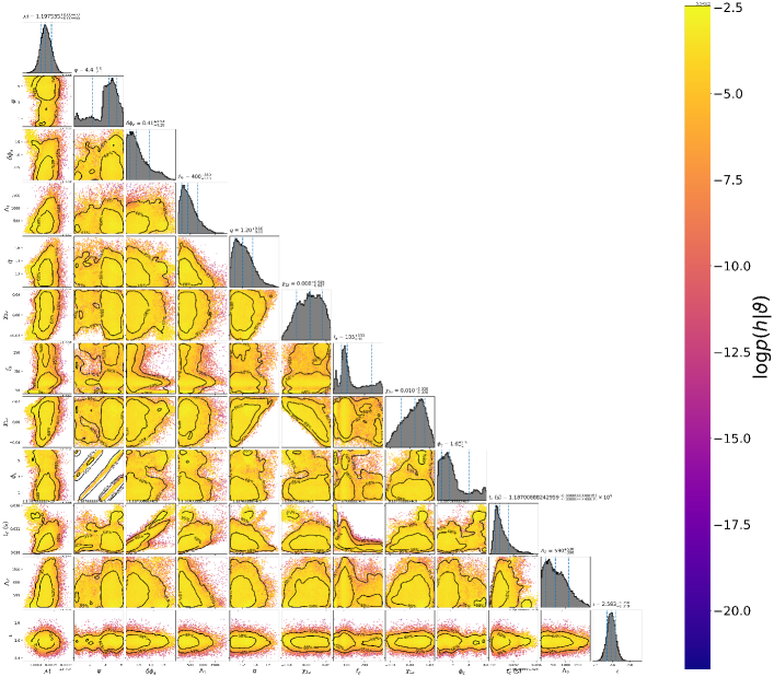
Figure 4: The posterior distribution of all parameters in the search of mode resonance presented in Fig. 3a in the maintext with data from GW170817.

For the search of possible mode resonance in GW170817, we have incorporated $\delta\phi_{a},f_{a}$ plus all the binary parameters (except for the source distance and sky location which are known from electromagnetic counterparts), including chirp mass $\mathcal{M}$, mass ratio $q$, inclination angle $\iota$, polarization phase $\psi_{c}$, coalescence phase $\phi_{c}$, coalescence time $t_{c}$, tidal Love numbers of both stars $\Lambda_{1,2}$ and parallel spins of both stars $\chi_{1,2z}$. The priors of the spin are set to be $|\chi_{1,2z}|<0.05$. The full posterior distribution of parameters and the Markov-Chain Monte-Carlo samples are presented in Fig. 4. In general, the accuracy of the search result not only depends on the event signal-to-noise ratio, but also on the melting frequency. If the melting frequency is too small, even if it is still in the LIGO band, the imbalance of the waveform signal-to-noise ratio before and after the melting process still degrades the search accuracy. For GW170817, given that the low-frequency sensitivity of the LIGO detectors in O2 is significantly worse than O3, we find that it is beneficial to set the lower bound of the frequency range to be at least 40 Hz to allow ${\rm SNR}\sim 5$ in the waveform before the resonance. This situation will be greatly improved as LIGO reaches design sensitivity when the low-frequency performance is much better, and definitely for LIGO A+ and 3rd-generation detectors, which is important as crust melting may happen before $40$ Hz.

To compare two models or hypotheses, we apply the Bayesian model selection method. For hypothesis $\mathcal{H}_{1}$ and $\mathcal{H}_{0}$ and observed data $s$, the Bayes factor is defined as

$$\mathcal{B}^{1}_{0}=\frac{P(s|\mathcal{H}_{1})}{P(s|\mathcal{H}_{0})}\,.$$ (16)

The probability functions ${P(s|\mathcal{H}_{0,1})}$ are usually referred to as the evidence, which may be computed with various tools, such as the thermodynamic integration method Lartillot and Philippe (2006) and the Savage-Dickey Density Ratio method Dickey (1971). Larger Bayes factor $\mathcal{B}^{1}_{0}$ implies more preference of hypothesis 1 over hypothesis 0, and vice versa. According to the justification in Kass and Raftery (1995), if $-1.1<\log\mathcal{B}^{1}_{0}<1.1$, the data does not prefer one model over the other; if $1.1<\log\mathcal{B}^{1}_{0}<3$, there is positive support for model 1; if $3<\log\mathcal{B}^{1}_{0}<5$, there is strong support for model 1 and if $\log\mathcal{B}^{1}_{0}>5$, the support is overwhelming. We have applied such formalism in the search for a resonance signature in the data of GW170817, in which case $\mathcal{H}_{1}$ is the model including the resonance effect and the null hypothesis $\mathcal{H}_{0}$ is the one without. We obtain $\log\mathcal{B}^{1}_{0}\sim[-0.6,-0.3]$, so that there is no evidence of mode resonance in the parameter range we searched for in the strain data of GW170817.

For generality, we repeat the above Bayesian analysis imposing a wider prior $[-2,2]$ on $\delta\phi_{a}$ and a same prior $[30,300]$ Hz on $f_{a}$. As a result, we find all the model parameter constraints are consistent with what shown in the maintext (see Fig. 5).

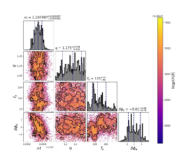
Figure 5: Posterior distribution in the search of mode resonance from data of GW170817 imposing a wider prior $[-2,2]$ on $\delta\phi_{a}$. All the parameter constraints are consistent with the result shown in Fig. 3a in the maintext.

Appendix C Model selection

The model selection method also applies to distinguish possible origins of the signal. For example, if we detect a signal by searching with our mode resonance waveform, it may also show a positive signal if we had searched for this signal with waveforms motivated by other reasons. To illustrate this, we injected a mode resonance signal ($\delta\phi_{a}=0.3,f_{a}=60$Hz) to simulated detector noise compatible with LIGO A+, and searched it with both our mode resonance waveform and the waveform for tidal-p-g coupling Abbott et al. (2019):

$$\delta\Psi(f) =-\frac{2C}{3B^{2}(3-n_{0})(4-n_{0})}\left\{\Theta\left(\frac{f}{f_{\rm ref}}\right)^{n_{0}-3}\right.$$

$$\left.+(1-\Theta)\left(\frac{f_{0}}{f_{\rm ref}}\right)^{n_{0}-3}\left[(4-n_{0})-(3-n_{0})\left(\frac{f}{f_{0}}\right)\right]\right\}\,,$$ (17)

where $\Theta=\Theta(f-f_{0})$, $f_{\rm ref}=100$Hz, $C=A_{0}[(2m_{1})^{2/3}+(2m_{2})^{2/3}]/M^{2/3}$, and $B=(32/5)(G\mathcal{M}\pi f_{\rm ref})^{5/3}$. The corresponding posterior distributions of parameters are shown in  Fig. 6. The fitting with tidal-p-g coupling does not generate a compact posterior distribution of the parameters of this model, $A_{0},f_{0}$ and $n_{0}$, although the distribution of $\log A_{0}$ is significantly different from the lower bound of its prior, which is -10. As we compare the two models, the Bayes factor $\log\mathcal{B}^{\rm res}_{\rm pg}$ is $2.7\pm 0.3$, which shows a preference for the mode resonance model. This means that it is still possible to distinguish these two models when we detect a mode resonance signal with LIGO A+.

In the case of double NSs carrying scalar (e.g., axions with mass $m_{\rm s}$ Huang et al. (2019)) charge $q_{1}$ and $q_{2}$ , the BNS evolution would be modified by both the extra force mediated by the scalar and the extra scalar dipole radiation. To the leading order, the extra force can be described in term of Yukuwa potential $V_{\rm s}(r)=-8q_{1}q_{2}e^{-m_{\rm s}r}/r$ and scalar dipole emission power is $P_{\rm s}(r)=\frac{1}{12}\frac{(q_{1}m_{2}-q_{2}m_{1})^{2}}{M^{2}M^{2}_{\rm Planck}}\left(1-\frac{m_{s}^{2}}{\Omega^{2}}\right)^{3/2}r^{2}\Omega^{4}\Theta(\Omega^{2}-m_{s}^{2})$, where $M=m_{1}+m_{2}$ is the total mass of the BNS system, $\Omega(r)$ is the orbital frequency. For convenience, we define symmetry charge $q_{0}:=q_{1}q_{2}/m_{1}m_{2}$, anti-symmetry charge $\delta q_{0}:=q_{1}/m_{1}-q_{2}/m_{2}$ and dimensionless variable $\lambda_{0}:=(GMm_{s})^{-1}$. We find the GW phase shift driven the extra scalar degree of freedom is $\delta\Psi(f)=2\pi f\delta t_{\rm s}(f)-\delta\phi_{\rm s}(f)$, with

$$\delta\phi_{\rm s}(f) =\frac{5q_{0}\lambda_{0}^{5/2}}{12\eta}\Bigg{[}6\Gamma\left(\frac{5}{2},\frac{1}{\lambda_{0}v^{2}}\right)+2\Gamma\left(\frac{7}{2},\frac{1}{\lambda_{0}v^{2}}\right)$$ (18)

$$-\Gamma\left(\frac{9}{2},\frac{1}{\lambda_{0}v^{2}}\right)\Bigg{]}+\Bigg{[}\frac{25(\delta q_{0})^{2}}{1344\eta v^{7}}\ _{2}F_{1}\left(-\frac{1}{2},\frac{7}{6},\frac{13}{6},\frac{1}{\lambda_{0}^{2}v^{6}}\right)$$

$$-\frac{25(\delta q_{0})^{2}}{2496\eta\lambda_{0}^{2}v^{13}}\ _{2}F_{1}\left(-\frac{1}{2},\frac{13}{6},\frac{19}{6},\frac{1}{\lambda_{0}^{2}v^{6}}\right)-C_{1}\Bigg{]}\Theta\ ,$$

$$\delta t_{\rm s}(f) =\frac{5q_{0}\lambda_{0}^{4}v^{3}}{24\eta\Omega}\Bigg{[}6\Gamma\left(4,\frac{1}{\lambda_{0}v^{2}}\right)+2\Gamma\left(5,\frac{1}{\lambda_{0}v^{2}}\right)$$

$$-\Gamma\left(6,\frac{1}{\lambda_{0}v^{2}}\right)\Bigg{]}+\Bigg{[}\frac{5(\delta q_{0})^{2}}{768\eta\Omega v^{7}}\ _{2}F_{1}\left(-\frac{1}{2},\frac{5}{3},\frac{8}{3},\frac{1}{\lambda_{0}^{2}v^{6}}\right)$$

$$-\frac{25(\delta q_{0})^{2}}{6144\eta\Omega\lambda_{0}^{2}v^{13}}\ _{2}F_{1}\left(-\frac{1}{2},\frac{8}{3},\frac{11}{3},\frac{1}{\lambda_{0}^{2}v^{6}}\right)-C_{2}\Bigg{]}\Theta\ ,$$

where $\Theta:=\Theta(f-\frac{1}{\pi GM\lambda_{0}})$, $v(f):=(GM\Omega)^{1/3}=(GM\pi f)^{1/3}$, $\Gamma(a,z):=\int_{z}^{\infty}t^{a-1}e^{-t}dt$ is the gamma function, ${}_{2}F_{1}$ is the hypergeometric function, and $C_{1,2}$ are two integration constants enabling vanishing $\delta t_{\rm s}$ and $\delta\phi_{\rm s}$ at $f=\frac{1}{\pi GM\lambda_{0}}$. To illustrate the power of LIGO A+ distinguishing the scalar dipole radiation from the mode resonance, we also constrain the scalar radiation model using the same mock data above (Fig. 7) and we find the Bayes factor $\ln\mathcal{B}^{\rm res}_{\rm dipole}=11.7\pm 2.2$.

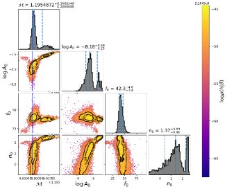
Figure 6: The posterior distribution of chirp mass $\mathcal{M}$, and $A_{0},n_{0},f_{0}$ as we try to fit the mock data with the tidal-p-g mode waveform.

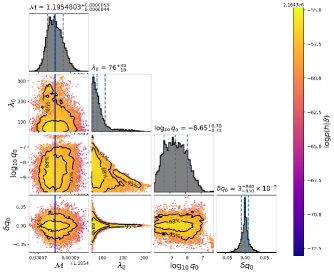
Figure 7: The posterior distribution of chirp mass $\mathcal{M}$, and $\lambda_{0},q_{0},\delta q_{0}$ as we try to fit the mock data with the waveform of scalar dipole radiation.

References

- Flanagan and Hinderer (2008) E. E. Flanagan and T. Hinderer, Phys. Rev. D77, 021502 (2008), arXiv:0709.1915 [astro-ph] .
- Abbott et al. (2018) B. P. Abbott et al. (LIGO Scientific, Virgo), Phys. Rev. Lett. 121, 161101 (2018), arXiv:1805.11581 [gr-qc] .
- Miller et al. (2019) M. C. Miller et al., Astrophys. J. Lett. 887, L24 (2019), arXiv:1912.05705 [astro-ph.HE] .
- Rezzolla et al. (2018) L. Rezzolla, E. R. Most, and L. R. Weih, Astrophys. J. 852, L25 (2018), arXiv:1711.00314 [astro-ph.HE] .
- Radice et al. (2018) D. Radice, A. Perego, F. Zappa, and S. Bernuzzi, Astrophys. J. 852, L29 (2018), arXiv:1711.03647 [astro-ph.HE] .
- Kokkotas and Schmidt (1999) K. D. Kokkotas and B. G. Schmidt, Living Reviews in Relativity 2, 2 (1999), arXiv:gr-qc/9909058 [gr-qc] .
- Pratten et al. (2019) G. Pratten, P. Schmidt, and T. Hinderer, (2019), arXiv:1905.00817 [gr-qc] .
- Lai (1994) D. Lai, MNRAS 270, 611 (1994), arXiv:astro-ph/9404062 [astro-ph] .
- Yu and Weinberg (2017) H. Yu and N. N. Weinberg, Mon. Not. Roy. Astron. Soc. 464, 2622 (2017), arXiv:1610.00745 [astro-ph.HE] .
- Ho and Lai (1999) W. C. G. Ho and D. Lai, Mon. Not. Roy. Astron. Soc. 308, 153 (1999), arXiv:astro-ph/9812116 [astro-ph] .
- Lai and Wu (2006) D. Lai and Y. Wu, Phys. Rev. D74, 024007 (2006), arXiv:astro-ph/0604163 [astro-ph] .
- Flanagan and Racine (2007a) E. E. Flanagan and E. Racine, Phys. Rev. D75, 044001 (2007a), arXiv:gr-qc/0601029 [gr-qc] .
- Poisson (2020) E. Poisson, arXiv e-prints , arXiv:2003.10427 (2020), arXiv:2003.10427 [gr-qc] .
- Burgay et al. (2003) M. Burgay et al., Nature 426, 531 (2003), arXiv:astro-ph/0312071 [astro-ph] .
- Andrews and Mandel (2019) J. J. Andrews and I. Mandel, Astrophys. J. Lett. 880, L8 (2019), arXiv:1904.12745 [astro-ph.HE] .
- McDermott et al. (1985) P. N. McDermott, C. J. Hansen, H. M. van Horn, and R. Buland , Astrophys. J. Lett. 297, L37 (1985).
- McDermott et al. (1988) P. N. McDermott, H. M. van Horn, and C. J. Hansen, Astrophys. J. 325, 725 (1988).
- Tsang et al. (2012) D. Tsang, J. S. Read, T. Hinderer, A. L. Piro, and R. Bondarescu, Phys. Rev. Lett. 108, 011102 (2012), arXiv:1110.0467 [astro-ph.HE] .
- Strohmayer et al. (1991) T. Strohmayer, S. Ogata, H. Iyetomi, S. Ichimaru, and H. M. van Horn, Astrophys. J. 375, 679 (1991).
- Ravenhall et al. (1983) D. G. Ravenhall, C. J. Pethick, and J. R. Wilson, Phys. Rev. Lett. 50, 2066 (1983).
- Hashimoto et al. (1984) M.-a. Hashimoto, H. Seki, and M. Yamada, Progress of Theoretical Physics 71, 320 (1984).
- Chugunov and Horowitz (2010) A. I. Chugunov and C. J. Horowitz, MNRAS 407, L54 (2010), arXiv:1006.2279 [astro-ph.SR] .
- Thompson et al. (2017) C. Thompson, H. Yang, and N. Ortiz, Astrophys. J. 841, 54 (2017), arXiv:1608.02633 [astro-ph.HE] .
- Chabrier (1993) G. Chabrier, Astrophys. J. 414, 695 (1993).
- Shapiro and Teukolsky (1983) S. L. Shapiro and S. A. Teukolsky, Black holes, white dwarfs, and neutron stars : the physics of compact objects, New York: Wiley (1983).
- (26) “See Supplemental Material at [ ] for the derivation of the pulsation equations and the mode search details,” .
- Douchin and Haensel (2001) F. Douchin and P. Haensel, Astronomy & Astrophysics 380, 151 (2001), arXiv:astro-ph/0111092 [astro-ph] .
- Read et al. (2009) J. S. Read, B. D. Lackey, B. J. Owen, and J. L. Friedman, Phys. Rev. D 79, 124032 (2009).
- Note (1) In Ref. Tsang et al. (2012), a factor was missed in the normalization calculation.
- Passamonti and Andersson (2012) A. Passamonti and N. Andersson, MNRAS 419, 638 (2012), arXiv:1105.4787 [astro-ph.SR] .
- Flanagan and Racine (2007b) E. E. Flanagan and E. Racine, Phys. Rev. D 75, 044001 (2007b).
- Horowitz and Piekarewicz (2001) C. J. Horowitz and J. Piekarewicz, Phys. Rev. Lett. 86, 5647 (2001), arXiv:astro-ph/0010227 [astro-ph] .
- Xu et al. (2009) J. Xu, L.-W. Chen, B.-A. Li, and H.-R. Ma, Astrophys. J. 697, 1549 (2009), arXiv:0901.2309 [astro-ph.SR] .
- Moustakidis et al. (2010) C. C. Moustakidis, T. Nikšić, G. A. Lalazissis, D. Vretenar, and P. Ring, Phys. Rev. C 81, 065803 (2010), arXiv:1004.3882 [nucl-th] .
- Cowling (1941) T. G. Cowling, MNRAS 101, 367 (1941).
- Yoshida and Kojima (1997) S. Yoshida and Y. Kojima, MNRAS 289, 117 (1997), arXiv:gr-qc/9705081 [gr-qc] .
- Chirenti et al. (2015) C. Chirenti, G. H. de Souza, and W. Kastaun, Phys. Rev. D 91, 044034 (2015).
- Brown et al. (2018) E. F. Brown, A. Cumming, F. J. Fattoyev, C. J. Horowitz, D. Page, and S. Reddy, Phys. Rev. Lett. 120, 182701 (2018).
- Abbott et al. (2019) B. P. Abbott et al. (LIGO Scientific, Virgo), Phys. Rev. Lett. 122, 061104 (2019), arXiv:1808.08676 [astro-ph.HE] .
- Biwer et al. (2019) C. M. Biwer, C. D. Capano, S. De, M. Cabero, D. A. Brown, A. H. Nitz, and V. Raymond, PASP 131, 024503 (2019), arXiv:1807.10312 [astro-ph.IM] .
- Abbott et al. (2017) B. P. Abbott, R. Abbott, T. Abbott, F. Acernese, K. Ackley, C. Adams, T. Adams, P. Addesso, R. Adhikari, V. Adya, et al., Physical Review Letters 119, 161101 (2017).
- Buonanno et al. (2009) A. Buonanno, B. Iyer, E. Ochsner, Y. Pan, and B. S. Sathyaprakash, Phys. Rev. D80, 084043 (2009), arXiv:0907.0700 [gr-qc] .
- Lartillot and Philippe (2006) N. Lartillot and H. Philippe, Systematic Biology 55, 195 (2006), https://academic.oup.com/sysbio/article-pdf/55/2/195/26557316/10635150500433722.pdf .
- Dickey (1971) J. M. Dickey, The Annals of Mathematical Statistics 42, 204 (1971).
- Kass and Raftery (1995) R. E. Kass and A. E. Raftery, Journal of the American Statistical Association 90, 773 (1995).
- Note (2) https://dcc.ligo.org/LIGO-G1601435/public.
- Yang et al. (2017) H. Yang, K. Yagi, J. Blackman, L. Lehner, V. Paschalidis, F. Pretorius, and N. Yunes, Phys. Rev. Lett. 118, 161101 (2017), arXiv:1701.05808 [gr-qc] .
- Palenzuela et al. (2014) C. Palenzuela, E. Barausse, M. Ponce, and L. Lehner, Phys. Rev. D89, 044024 (2014), arXiv:1310.4481 [gr-qc] .
- Annulli et al. (2019) L. Annulli, V. Cardoso, and L. Gualtieri, Phys. Rev. D99, 044038 (2019), arXiv:1901.02461 [gr-qc] .
- Mendes and Ortiz (2018) R. F. Mendes and N. Ortiz, Physical Review Letters 120 (2018), 10.1103/physrevlett.120.201104.
- Huang et al. (2019) J. Huang, M. C. Johnson, L. Sagunski, M. Sakellariadou, and J. Zhang, Phys. Rev. D 99, 063013 (2019).
- Abbott et al. (2017) B. P. Abbott, R. Abbott, T. D. Abbott, M. R. Abernathy, K. Ackley, C. Adams, P. Addesso, R. X. Adhikari, V. B. Adya, C. Affeldt, and et al., Classical and Quantum Gravity 34, 044001 (2017), arXiv:1607.08697 [astro-ph.IM] .
- Punturo et al. (2010) M. Punturo et al., Proceedings, 14th Workshop on Gravitational wave data analysis (GWDAW-14): Rome, Italy, January 26-29, 2010, Class. Quant. Grav. 27, 194002 (2010).
- Ackermann et al. (2009) M. Ackermann et al. (Fermi GBM/LAT), Nature 462, 331 (2009), arXiv:0908.1832 [astro-ph.HE] .
- Troja et al. (2010) E. Troja, S. Rosswog, and N. Gehrels, Astrophys. J. 723, 1711 (2010), arXiv:1009.1385 [astro-ph.HE] .
- The LIGO Scientific Collaboration et al. (2020) The LIGO Scientific Collaboration, the Virgo Collaboration, B. P. Abbott, R. Abbott, T. D. Abbott, S. Abraham, F. Acernese, K. Ackley, C. Adams, R. X. Adhikari, V. B. Adya, C. Affeldt, M. Agathos, K. Agatsuma, N. Aggarwal, O. D. Aguiar, L. Aiello, A. Ain, P. Ajith, G. Allen, A. Allocca, M. A. Aloy, P. A. Altin, A. Amato, S. Anand, A. Ananyeva, S. B. Anderson, W. G. Anderson, S. V. Angelova, S. Antier, S. Appert, K. Arai, M. C. Araya, J. S. Areeda, M. Arène, N. Arnaud, S. M. Aronson, K. G. Arun, S. Ascenzi, G. Ashton, S. M. Aston, P. Astone, F. Aubin, P. Aufmuth, K. AultONeal, C. Austin, V. Avendano, A. Avila-Alvarez, S. Babak, P. Bacon, F. Badaracco, M. K. M. Bader, S. Bae, J. Baird, P. T. Baker, F. Baldaccini, G. Ballardin, S. W. Ballmer, A. Bals, S. Banagiri, J. C. Barayoga, C. Barbieri, S. E. Barclay, B. C. Barish, D. Barker, K. Barkett, S. Barnum, F. Barone, B. Barr, L. Barsotti, M. Barsuglia, D. Barta, J. Bartlett, I. Bartos, R. Bassiri, A. Basti, M. Bawaj, J. C. Bayley, A. C. Baylor, M. Bazzan, B. Bécsy, M. Bejger, I. Belahcene, A. S. Bell, D. Beniwal, M. G. Benjamin, B. K. Berger, G. Bergmann, S. Bernuzzi, C. P. L. Berry, D. Bersanetti, A. Bertolini, J. Betzwieser, R. Bhandare, J. Bidler, E. Biggs, I. A. Bilenko, S. A. Bilgili, G. Billingsley, R. Birney, O. Birnholtz, S. Biscans, M. Bischi, S. Biscoveanu, A. Bisht, M. Bitossi, M. A. Bizouard, J. K. Blackburn, J. Blackman, C. D. Blair, D. G. Blair, R. M. Blair, and S. e. a. Bloemen, (2020), arXiv:2001.01761 [astro-ph.HE] .
- Yang and Zou (2020) H. Yang and Y.-C. Zou, (2020), arXiv:2002.02553 [astro-ph.HE] .