Deep Learning Algorithms for Rotating Machinery Intelligent Diagnosis: An Open Source Benchmark Study

Abstract

Rotating machinery intelligent diagnosis based on deep learning (DL) has gone through tremendous progress, which can help reduce costly breakdowns. However, different datasets and hyper-parameters are recommended to be used, and few open source codes are publicly available, resulting in unfair comparisons and ineffective improvement. To address these issues, we perform a comprehensive evaluation of four models, including multi-layer perception (MLP), auto-encoder (AE), convolutional neural network (CNN), and recurrent neural network (RNN), with seven datasets to provide a benchmark study. We first gather nine publicly available datasets and give a comprehensive benchmark study of DL-based models with two data split strategies, five input formats, three normalization methods, and four augmentation methods. Second, we integrate the whole evaluation codes into a code library and release it to the public for better comparisons. Third, we use specific-designed cases to point out the existing issues, including class imbalance, generalization ability, interpretability, few-shot learning, and model selection. Finally, we release a unified code framework for comparing and testing models fairly and quickly, emphasize the importance of open source codes, provide the baseline accuracy (a lower bound), and discuss existing issues in this field. The code library is available at: https://github.com/ZhaoZhibin/DL-based-Intelligent-Diagnosis-Benchmark.

left=2.0cm,right=2.0cm,top=2.0cm,bottom=2.0cm

1 Introduction

Rotating machinery, as key mechanical equipment in the modern industry, is chronically running in a complex environment with elevated temperature, fatigue, and heavy load. Generated faults might cause severe accidents, resulting in enormous economic loss and casualties. Intelligent diagnosis, as a key ingredient of prognostics health management (PHM), which is one of the most essential systems in a wide range of rotating machinery, such as helicopter, aero-engine, wind turbine, and high-speed train, is designed to detect faults effectively. Traditional intelligent diagnosis methods mainly consist of feature extraction using signal processing methods [1, 2] and fault classification [3] using machine learning approaches, which have made considerable progress. However, facing with heterogeneous massive data, feature extraction methods and mapping abilities from signals to conditions that are designed and chosen by experts, to a great extent depending on prior knowledge, are time-consuming and empirical. Thus, how to perform diagnosis more precisely and efficiently is still a challenging problem.

DL, as a booming data mining technique, has swept many fields including computer vision (CV) [4, 5], natural language processing (NLP) [6, 7, 8], and other fields [9, 10]. In 2006, the concept of DL was first introduced via proposing deep belief network (DBN) [11]. In 2013, MIT Technology Review ranked the DL technology as the top ten breakthrough technologies [12]. In 2015, a review [13] published in nature stated that DL allows computational models composed of multiple processing layers to learn data representations with multiple levels of the abstraction. Due to its strong representation learning ability, DL is well-suited to data analysis and classification. Therefore, in the field of intelligent diagnosis, many researchers have applied DL-based techniques, such as multi-layer perception (MLP), auto-encoder (AE), convolutional neural network (CNN), DBN, and recurrent neural network (RNN) to boost the performance. However, different researchers often recommended to use different inputs (such as time domain input, frequency domain input, time-frequency domain input, etc.) and set different hyper-parameters (such as the learning rate, the batch size, the network architecture, etc.). Unfortunately, a few authors made their codes available for comparisons, resulting in unfair comparisons and ineffective improvement. To address this problem, it is crucial to evaluate and compare different DL-based intelligent diagnosis algorithms to provide the benchmark study and open souce codes, thereby helping further studies to propose more persuasive and appropriate algorithms.

For comprehensive performance comparisons, it is necessary to collect different datasets in a library and evaluate the performance of algorithms for different datasets on a unified platform. In addition, one common issue in intelligent diagnosis is data split, and researchers often use the random split strategy. This strategy is dangerous since if the preparation process exists any overlap, the evaluation of classification algorithms will have test leakage [14]. As for industrial data, they are rarely random and are always sequential (they might contain trends in the time domain), and it is more appropriate to split data according to time sequences (we simply call it order split). Conversely, if we randomly split the data, it might be possible for diagnosis algorithms to record the future patterns, which might cause another pitfall with test leakage.

To address these problems, in this paper, we collect nine publicly available datasets and discuss whether it is suitable for intelligent diagnosis. After that, we evaluate DL-based intelligent diagnosis algorithms from different perspectives including the data preparation for all datasets and the whole evaluation framework with different input formats, normalization methods, data split ways, augmentation methods, and DL-based models. Based on the benchmark study, we highlight some evaluation results which are very important for comparing or testing new models. First, not all datasets are suitable for comparing the classification effectiveness of the proposed methods since basic models can achieve very high accuracy on these datasets, like CWRU and XJTU-SY. Second, the frequency domain input can achieve the highest accuracy in all datasets, so researchers should first try to use the frequency domain as the input. Third, it is not necessary for CNN models to get the best results in all cases, and we also should consider the overfitting problem. Fourth, when the accuracy of datasets is not very high, data augmentation methods improve the performance of models, especially for the time domain input. Thus, more effective data augmentation methods need to be investigated. Finally, in some cases, it may be more suitable for splitting the datasets according to time sequences (order split) since the random split may provide a virtually high accuracy. We also release a code library to evaluate DL-based intelligent diagnosis algorithms and provide the benchmark accuracy (a lower bound) to avoid useless improvement. Meanwhile, we use specific-designed cases to discuss existing issues, including class imbalance, generalization ability, interpretability, few-shot learning, and model selection. Through these works, we aim to allow comparisons fairer and quicker, emphasize the importance of open source codes, and provide deep discussions of existing issues. To the best of our knowledge, this is the first work to comprehensively perform the benchmark study and release the code library to the public. The code library is available at: https://github.com/ZhaoZhibin/DL-based-Intelligent-Diagnosis-Benchmark.

The main contributions of this paper can be summarized as three aspects:

1. Various datasets and data preparing. We gather nine publicly available datasets and give a detailed discussion about its adaptability. For data preparation, we first discuss different kinds of input formats and normalization methods, and then we perform different data augmentation approaches to clarify that they have not been fully investigated. We also discuss the way of data split and state that it may be more appropriate to split data according to time sequences.

2. Benchmark accuracy and existing issues. We evaluate various DL-based intelligent diagnosis algorithms for seven datasets and provide the benchmark accuracy to make future studies more comparable. Based on the benchmark study, we highlight some evaluation results which are very important for comparing or testing new models. We also discuss the existing issues, including class imbalance, generalization ability, interpretability, few-shot learning, and model selection.

3. Open source codes. To emphasize the reproducibility of DL-based intelligent diagnosis algorithms, we release the code library for the better comparisons. Meanwhile, it is a unified intelligent diagnosis library, which retains an extended interface for everyone to load their own datasets and models to carry out new studies.

The outlines of this paper are listed as follows: In Section 2, we give a brief review of the recent development of DL-based intelligent diagnosis algorithms. Then, Sections 3 to 9 discuss the evaluation algorithms, datasets, data preprocessing, data augmentation, data split, evaluation methodologies, and evaluation results, respectively. After that, Section 10 makes some further discussions and the results, followed by conclusions in Section 11.

2 Brief Review

Recently, DL has become a promising method in a large scope of fields, and a huge amount of papers related to DL have been published since 2012. This paper mainly focuses on a benchmark study of intelligent diagnosis, rather than providing a comprehensive review on DL for other fields. Some famous DL researchers have published more professional references, and readers could refer to [13, 15].

Due to the efforts of many researchers, DL has become one of the most popular data-driven methods to perform intelligent diagnosis. In general, DL-based methods can extract representative features adaptively without any manual intervention and can achieve a higher accuracy than traditional machine learning algorithms in most of the tasks when the dataset is large enough. We conducted a literature search using Web of Science with a database called web of science core collection. As shown in Fig. 1, we can observe that the number of published papers related to DL-based intelligent algorithms increases year by year.

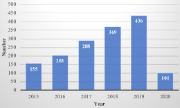
Figure 1: The relationship between the number of published papers and publication years covering the last six years (as of April 2020). The basic descriptor is “TI= ((deep OR autoencoder OR convolutional network* OR neural network*) AND (fault OR condition monitoring OR health management OR intelligent diagnosis))”.

Another interesting observation is that many review papers on this topic have been published in the recent four years. Therefore, in this paper, we first summarize the main contents of different review papers, allowing readers who just enter this field to find suitable review papers quickly.

In bearing fault diagnosis, Li et al. [16] provided a systematic review of fuzzy formalisms including combination with other machine learning algorithms. Hoang et al. [17] provided a comprehensive review of three popular DL algorithms (AE, DBN, and CNN) for bearing fault diagnosis. Zhang et al. [18] systematically reviewed the machine learning and DL-based algorithms for bearing fault diagnosis and also provided a comparison of the classification accuracy of CWRU with different DL-based methods. Hamadache et al. [19] reviewed different fault modes of rolling element bearings and described various health indexes for PHM. Meanwhile, it also provided a survey of artificial intelligence (AI) methods for PHM including shallow learning and DL.

In rotating machinery intelligent diagnosis, Ali et al. [20] provided a review of AI-based methods using acoustic emission data for rotating machinery condition monitoring. Liu et al. [21] reviewed Al-based approaches including k-nearest neighbors (KNN), support vector machine (SVM), artificial neural networks (ANN), Naive Bayes, and DL for fault diagnosis of rotating machinery. Wei et al. [22] summarized early fault diagnosis of gears, bearings, and rotors through signal processing methods (adaptive decomposition methods, wavelet transform, and sparse decomposition) and AI-based methods (KNN, neural network, and SVM).

In machinery condition monitoring, Zhao et al. [23] and Duan et al. [24] reviewed diagnosis and prognosis of mechanical equipment based on DL algorithms such as DBN and CNN. Zhang et al. [25] reviewed computational intelligent approaches including ANN, evolutionary algorithms, fuzzy logic, and SVM for machinery fault diagnosis. Zhao et al. [26] reviewed data-driven machine health monitoring through DL methods (AE, DBN, CNN, and RNN) and provided the data and codes (in Keras) about an experimental study. Lei et al. [27] presented a systematical review to cover the development of intelligent diagnosis following the progress of machine learning and DL models and offer a future perspective called transfer learning theories.

In addition, Nasiri et al. [28] surveyed the state-of-the-art AI-based approaches for fracture mechanics and provided the accuracy comparisons achieved by different machine learning algorithms for mechanical fault detection. Tian et al. [29] surveyed different modes of traction induction motor fault and their diagnosis algorithms including model-based methods and AI-based methods. Khan et al. [30] provided a comprehensive review of AI for system health management and emphasized the trend of DL-based methods with limitations and benefits. Stetco et al. [31] reviewed machine learning approaches applied to wind turbine condition monitoring and made a discussion of the possibility for future research. Ellefsen et al. [32] reviewed four well-established DL algorithms including AE, CNN, DBN, and long short-term memory network (LSTM) for PHM applications and discussed challenges for the future studies, especially in the field of PHM in autonomous ships. AI-based algorithms (traditional machine learning algorithms and DL-based approaches) and applications (smart sensors, intelligent manufacturing, PHM, and cyber-physical systems) were reviewed in [33, 34, 35, 36] for smart manufacturing and manufacturing diagnosis.

Due to the fact that there are already many review papers covering DL-based rotating machinery intelligent diagnosis published before 2020, we further review most of related papers published in 2020 and summarize their main contributions to fill the void.

In AE models, for model improvement, AE models were combined with some other data preprocessing methods, such as singular value decomposition [37] and nonlinear frequency spectrum [38]. The ensemble learning strategy was also used to boost the performance of AE models in [39, 40]. Meanwhile, the semi-supervised learning methods were also embedded into AE models by [41, 42]. For imbalanced learning, generation adversarial network (GAN) was used to combine with AE models to generate new labeled samples in [43, 44, 45]. In [46], a model called deep Laplacian AE (DLapAE) was proposed by introducing the Laplacian regularization to improve the generalization performance. For transfer learning, the pretrained and fine-tuned approach was applied to AE models to realize the knowledge transfer in [47, 48]. Domain adaptation was also used to transfer the knowledge learned by AE models to the target domain in [49, 50].

In CNN models, for model improvement, different input types, such as time-frequency images [51], vibration spectrum images [52], infrared thermal images [53], and two-dimensional images [54], were used as the inputs of CNN models. Multiple wavelet regularizations [55], data augmentation methods [56], and information fusion technology [57] were also applied to improve the performance of CNN models. Hand-crafted features were combined with CNN features to boost the performance in [58]. For imbalanced learning, GAN was also used to combine with CNN models to generate new labeled samples in [59, 60]. Focal loss, which can deal with severe imbalanced problems, was used by [61] to allow CNN models to learn discriminative features. For transfer learning, the pretrained and fine-tuned approach was used to leverage the prior knowledge from the source task in [62, 63, 64]. Domain adaptation methods were also applied to allow CNN models to learn transferable features in [65, 66]. In addition, layer-wise relevance propagation was also used to understand how CNN models learn to distinguish different patterns [67].

Beyond that, complex wavelet packet energy moment entropy [68] and the grey wolf optimizer algorithm [69] were combined with an enhanced deep gated recurrent unit to improve the security of rotating machinery. Joint distribution adaptation was embedded into LSTM to realize learning transferable features in [70]. DBN models were also modified in [71, 72, 73] to improve the diagnosis performance of rotating machinery. Deep reinforcement learning was also used in intelligent fault diagnosis for rotating machinery in [74, 75]. Meanwhile, a deep graph convolutional network (DGCN) was first applied to rolling bearing fault diagnosis based on acoustic signals [76].

Although a large body of DL-based methods and many related reviews have been published in the field of intelligent diagnosis, few studies thoroughly evaluate various DL-based intelligent diagnosis algorithms for most of the publicly available datasets, provide the benchmark accuracy, and release the code library for complete evaluation procedures. For example, a simple code written in Keras was published in [26], which is not comprehensive enough for different datasets and models. The accuracy comparisons were provided in [18, 28] according to existing papers, but they were not comprehensive enough due to different configurations. Therefore, this paper is intended to make up for this gap and emphasize the importance of open source codes and the benchmark study.

3 Evaluation Algorithms

It is impossible to cover all the published models since there is currently no open source community in this field. Therefore, we switch to test the performance of four models (including MLP, AE, CNN, and RNN) via embedding some advanced techniques. It should be noted that DBN is also another commonly used DL model in intelligent diagnosis, but we do not add it to this code library due to that the fact the training way of DBN is much different from those four models.

3.1 MLP

MLP [77], which was a fully connected network with multiple hidden layers, was proposed in 1987 as the prototype of ANN. With such a simple structure, MLP can complete some easy classification tasks such as MNIST. However, as the task becomes more complex, it would be hard to train MLP because of the huge amount of parameters. MLP with five fully connected layers and five batch normalization layers is used in this paper for one dimension (1D) input data. The structure and parameters of this model are shown in Fig. 2. Besides, in Fig. 2, FC means the fully connected layer, BN means the Batch Normalization layer, and CE loss means the softmax cross-entropy loss.

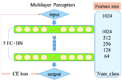
Figure 2: The structure of MLP.

3.2 AE

AE was first proposed in 2006, as a method for dimensionality reduction. It can reduce the dimensionality of the input data while retaining most of the information. AE consists of an encoder and a decoder, which tries to reconstruct the input from the output of an encoder, and the reconstruction error is used as a loss function. In detail, an encoder takes $x$ as an input and transforms it into a hidden representaion $h$ which can be formualted as:

$$h=\phi(W\cdot x+b)$$ (1)

$\phi(\cdot)$ denotes the nonlinear activation function (in this paper, we use ReLU), and $W$ and $b$ represent the weight and bias required to learn, respectively. After that, a decoder generates the output $x^{\prime}$ from the hidden representaion $h$, which can be formulated as:

$$x^{\prime}=\phi(W^{\prime}\cdot h+b^{\prime})$$ (2)

where $W^{\prime}$ and $b^{\prime}$ represent the weight and bias required to learn, respectively. For traditional AE, the mean squared error (MSE) loss is often used as a loss function, shown as follows:

$$L_{\text{MSE}}=\dfrac{1}{N}\sum\limits_{i=1}^{N}||x_{i}-x^{\prime}_{i}||^{2}_{2}$$ (3)

where $x_{i}$ and $x^{\prime}_{i}$ are the $i$-th sample and its approximation, respectively, and $N$ is the number of data samples. In practice, we often stack multiple layers in both encoder and decoder to produce better learning results.

Subsequently, various derivatives of AE were proposed by different researchers, such as denoising auto-encoder (DAE) [78] and sparse auto-encoder (SAE) [79]. In this paper, we design a deep AE and its derivatives for 1D input data (using the fully connected layer) and two dimension (2D) input data (using the convolutional layer), respectively. Considering different features of neural networks, the structures and hyper-parameters of them shown in Fig. 3 change adaptively. Specifically, the network structures of DAE and SAE are the same with AE, and their differences lie in the loss function and inputs. DAE takes an input corrupted with noise and is trained to reconstruct the clean version of the input; SAE uses a MSE loss regularized with a sparsity constraint (the Kullback-Leibler divergence is often used) to train the AE model. During the training of AE and its derivatives, the encoder and decoder are trained jointly to get the low-dimension features of data. After that, the encoder and classifier are trained jointly using the softmax cross-entropy loss for the classification task. The details of AE and its derivatives are shown in Fig. 3. In Fig. 3, the MSE loss means the mean square error loss defined in (3), Conv means the convolutional layer, $\text{Conv}^{\text{T}}$ means the transposed convolutional (e.g. inverse convolution) layer, and the KLP loss means the Kullback-Leibler divergence loss.

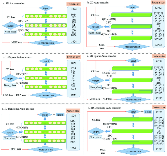
Figure 3: The structure of AE and its derivatives

3.3 CNN

CNN [80] was first proposed in 1997 and the proposed network was also called LeNet. CNN is a specialized kind of neural network for processing data that has a known grid-like topology. Sparse interactions, parameter sharing, and equivalent representations are realized with convolution and pooling operations on CNN. In 2012, AlexNet [4] won the title in the ImageNet competition by far surpassing the second place, and CNN has attracted wide attention. Besides, in 2016, ResNet [81] was proposed and its classification accuracy exceeded the human baseline. In this paper, we design 5 layers 1D CNN and 2D CNN for 1D input data and 2D input data, respectively, and also adapt three well known CNN models (LeNet, ResNet18, and AlexNet) for two types of the input data. The details of CNN and its derivatives are shown in Fig. 4. In Fig. 4, MaxPool means the Max Pooling layer, AdaptiveMaxPool means the Adaptive Max Pooling layer, and Dropout means the Dropout layer.

As shown in Fig. 4, CNN mainly contains three kinds of layers, including the convolutional layer, the maxpooling layer, and the classifier layer. Convolutional and maxpooling layers are utilized to perform feature learning, and the classifier layer classifies learned features into different classes. For an input $x$, the convolutional layer can be defined as a multiplication with a filter kernel $w$, and the final feature map after the nonlinear activation can be formulated as:

$$h_{k}^{l}=\phi(w_{k}^{l}*x+b_{k}^{l})$$ (4)

where $*$ denotes the convolution operator. $h_{k}^{l}$, $w_{k}^{l}$, and $b_{k}^{l}$ represent the obtained feature map, the weight and bias of $k$-th convolutional kernel of $l$-th layer, respectively.

The maxpooling layer is set behind the convolution layer to extract the most significant local information in each feature map and to reduce the dimension of obtained features. The maxpooling layer can be defined as:

$$z_{k}^{l}=\text{down}(h_{k}^{l};\;s)$$ (5)

where $\text{down}(\cdot)$ denotes the down-sampling function of the maxpooling layer, $z_{k}^{l}$ is the output feature map of the maxpooling layer, and $s$ is the pooling size.

After a number of stacked convolutional and pooling layers, the extracted high-level features of input data are input into the classifier layer. In this paper, a fully connected layer is used to map features into different classes.

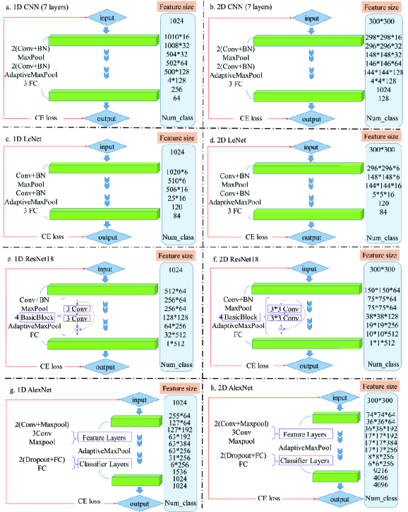
Figure 4: The structure of CNN and its derivatives

3.4 RNN

RNN can describe the temporal dynamic behavior and is very suitable for dealing with time series. However, RNN often exists the gradient vanishing and exploding problems during the training procedure. To overcome these problems, LSTM was proposed in 1997 [82] for processing continual input streams and has made great success in various fields. Bi-directional LSTM (BiLSTM) can capture bidirectional dependencies over long distances and learn to remember and forget information selectively. We utilize BiLSTM as the representation of RNN to deal with two types of input data (1D and 2D) for the classification task. The details of 1D BiLSTM and 2D BiLSTM are shown in Fig. 5. Besides, in Fig. 5, Transpose means transposing the channel and feature dimensions of the input data, and BiLSTM Block means the BiLSTM layer.

Figure 5: The structure of 1D BiLSTM and 2D BiLSTM

The structure of a LSTM cell is shown in Fig. 6, including the forget gate layer $\sigma_{1}$, the input gate layer $\sigma_{2}$, the output gate layer $\sigma_{3}$, and the tanh layer. Firstly, the hidden state of a last cell $h_{t-1}$ and the current input $x_{t}$ are fed into the forget gate layer to decide whether we should forget the last cell state $C_{t-1}$. Secondly, $h_{t-1}$ and $x_{t}$ are fed into the input gate layer and the tanh layer to decide values we want to update. Thirdly, $h_{t-1}$ and $x_{t}$ are fed into the output layer to decide what we should export for the last cell. Based on the structure shown in Fig. 6, the output cell state $C_{t}$ can be calculated as follows:

$$C_{t}=\sigma_{1}(h_{t-1},x_{t})\otimes C_{t-1}\oplus\sigma_{2}(h_{t-1},x_{t})\otimes\text{tanh}(h_{t-1},x_{t})$$ (6)

where $\otimes$ and $\oplus$ denote the element-wise multiplication and addition, respectively. Meanwhile, $\sigma_{i}(h_{t-1},x_{t})$ is defined as follows:

$$\sigma_{i}(h_{t-1},x_{t})=\sigma(W_{i}\cdot[h_{t-1},x_{t}]+b_{i}),\quad i=1,2,3$$ (7)

where $W_{i}$ and $b_{i}$ represent the weight and bias, respectively. $\sigma(\cdot)$ denotes the sigmoid function. Similarly, the tanh layer replaces the sigmoid function with the tanh function. In addition, the output hidden state $h_{t}$ can be calculate as follows:

$$h_{t}=\sigma_{3}(h_{t-1},x_{t})\otimes\text{tanh}(C_{t})$$ (8)

Many repeating cells are linked together to form a LSTM block, designed for capturing both long-term and short-term dependencies. The BiLSTM layer is the combining of forward and backward LSTM blocks, in which information is bidirectionally transmitted. For each input, information of the whole time series can be used simultaneously.

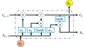
Figure 6: The structure of a LSTM cell

4 Datasets

In the field of intelligent diagnosis, publicly available datasets have not been investigated in depth. Actually, for comprehensive performance comparisons, it is important to gather different kinds of representative datasets. We collected nine commonly used datasets which all have specific labels and explanations in addition to the PHM 2012 bearing dataset and Intelligent Maintenance Systems (IMS) bearing dataset, so PHM 2012 and IMS are not suitable for fault classification that requires labels. To sum up, this paper uses seven datasets to verify the performance of models introduced in Section 3. The description of all these datasets is listed as follows.

4.1 CWRU Bearing Dataset

Case Western Reserve University (CWRU) datasets were provided by the Case Western Reserve University Bearing Data Center [83]. Vibration signals were collected at 12 kHz or 48 kHz for normal bearings and damaged bearings with single-point defects under four different motor loads. Within each working condition, single-point faults were introduced with fault diameters of 0.007, 0.014, and 0.021 inches on the rolling element, the inner ring, and the outer ring, respectively. In this paper, we used the data collected from the drive end, and the sampling frequency was equivalent to 12 kHz. In Table 1, one healthy bearing and three fault modes, including the inner ring fault, the rolling element fault, and the outer ring fault, were classified into ten categories (one health state and 9 fault states) according to different fault sizes.

Table 1: Detailed description of CWRU datasets

Fault Mode	Description
Health State	the normal bearing at 1791 rpm and 0 HP
Inner ring 1	0.007 inch inner ring fault at 1797 rpm and 0 HP
Inner ring 2	0.014 inch inner ring fault at 1797 rpm and 0 HP
Inner ring 3	0.021 inch inner ring fault at 1797 rpm and 0 HP
Rolling Element 1	0.007 inch rolling element fault at 1797 rpm and 0 HP
Rolling Element 2	0.014 inch rolling element fault at 1797 rpm and 0 HP
Rolling Element 3	0.021 inch rolling element fault at 1797 rpm and 0 HP
Outer ring 1	0.007 inch outer ring fault at 1797rpm and 0 HP
Outer ring 2	0.014 inch outer ring fault at 1797rpm and 0 HP
Outer ring 3	0.021 inch outer ring fault at 1797rpm and 0 HP

4.2 MFPT Bearing Dataset

Machinery Failure Prevention Technology (MFPT) datasets were provided by Society for Machinery Failure Prevention Technology [84]. MFPT datasets consisted of three bearing datasets: 1) a baseline dataset sampled at 97656 Hz for six seconds in each file; 2) seven outer ring fault datasets sampled at 48828 Hz for three seconds in each file; 3) seven inner ring fault datasets sampled at 48828 Hz for three seconds in each file; 4) some other datasets which were not used in this paper (more detailed information can be referred to the website of MFPT datasets [84]). In Table 2, one health state bearing and two fault bearings including the inner ring fault and the rolling element fault were classified into 15 categories (one health state and 14 fault states) according to different loads.

Table 2: Detailed description of MFPT datasets

Fault Mode	Description
Health State	Fault-free bearing working at 270 lbs
Outer ring 1	Outer ring fault bearing working at 25 lbs
Outer ring 2	Outer ring fault bearing working at 50 lbs
Outer ring 3	Outer ring fault bearing working at 100 lbs
Outer ring 4	Outer ring fault bearing working at 150 lbs
Outer ring 5	Outer ring fault bearing working at 200 lbs
Outer ring 6	Outer ring fault bearing working at 250 lbs
Outer ring 7	Outer ring fault bearing working at 300 lbs
Outer ring 1	Inner ring fault bearing working at 0 lbs
Inner ring 2	Inner ring fault bearing working at 50 lbs
Inner ring 3	Inner ring fault bearing working at 100 lbs
Inner ring 4	Inner ring fault bearing working at 150 lbs
Inner ring 5	Inner ring fault bearing working at 200 lbs
Inner ring 6	Inner ring fault bearing working at 250 lbs
Inner ring 7	Inner ring fault bearing working at 300 lbs

4.3 PU Bearing Dataset

Paderborn University (PU) datasets were provided by the Paderborn University Bearing Data Center [85, 86], and PU datasets consisted of 32 sets of current signals and vibration signals. As shown in Table 3, bearings were divided into: 1) six undamaged bearings; 2) twelve artificially damaged bearings; 3) fourteen bearings with real damages caused by accelerated lifetime tests. Each dataset was collected under four working conditions as shown in Table 4.

Table 3: Detailed description of PU datasets (S: single damage; R: repetitive damage; M: multiple damage)

Bearing Code	Fault Mode	Description	Bearing Code	Fault Mode	Description
K001	Health state	Run-in 50 h before test	KI07	Artificial inner ring fault (Level 2)	Made by electric engraver
K002	Health state	Run-in 19 h before test	KI08	Artificial inner ring fault (Level 2)	Made by electric engraver
K003	Health state	Run-in 1 h before test	KA04	Outer ring damage (single point + S + Level 1)	Caused by fatigue and pitting
K004	Health state	Run-in 5 h before test	KA15	Outer ring damage (single point + S + Level 1)	Caused by plastic deform and indentation
K005	Health state	Run-in 10 h before test	KA16	Outer ring damage (single point + R + Level 2)	Caused by fatigue and pitting
K006	Health state	Run-in 16 h before test	KA22	Outer ring damage (single point + S + Level 1)	Caused by fatigue and pitting
KA01	Artificial outer ring fault (Level 1)	Made by EDM	KA30	Outer ring damage (distributed + R + Level 1)	Caused by plastic deform and indentation
KA03	Artificial outer ring fault (Level 2)	Made by electric engraver	KB23	Outer ring and inner ring damage (single point + M + Level 2)	Caused by fatigue and pitting
KA05	Artificial outer ring fault (Level 1)	Made by electric engraver	KB24	Outer ring and inner ring damage (distributed + M + Level 3)	Caused by fatigue and pitting
KA06	Artificial outer ring fault (Level 2)	Made by electric engraver	KB27	Outer ring and inner ring damage (distributed + M + Level 1)	Caused by plastic deform and indentation
KA07	Artificial outer ring fault (Level 1)	Made by drilling	KI04	Inner ring damage (single point + M + Level 1)	Caused by fatigue and pitting
KA08	Artificial outer ring fault (Level 2)	Made by drilling	KI14	Inner ring damage (single point + M + Level 1)	Caused by fatigue and pitting
KA09	Artificial outer ring fault (Level 2)	Made by drilling	KI16	Inner ring damage (single point + S + Level 3)	Caused by fatigue and pitting
KI01	Artificial inner ring fault (Level 1)	Made by EDM	KI17	Inner ring damage (single point + R + Level 1)	Caused by fatigue and pitting
KI03	Artificial inner ring fault (Level 1)	Made by electric engraver	KI18	Inner ring damage (single point + S + Level 2)	Caused by fatigue and pitting
KI05	Artificial inner ring fault (Level 1)	Made by electric engraver	KI21	Inner ring damage (single point + S + Level 1)	Caused by fatigue and pitting

Table 4: Four working conditions of PU datasets

No.	Rotating speed (rpm)	Load torque (Nm)	Radial force (N)	Name of setting
0	1500	0.7	1000	N15_M07_F10
1	900	0.7	1000	N09_M07_F10
2	1500	0.1	1000	N15_M01_F10
3	1500	0.7	400	N15_M07_F04

In this paper, since using all the data would cause huge computational time, we only used the data collected from real damaged bearings (including KA04, KA15, KA16, KA22, KA30, KB23, KB24, KB27, KI14, KI16, KI17, KI18, and KI22) under the working condition N15_M07_F10 to carry out the performance verification. Since KI04 was the same as KI14 completely shown in Table 3, we deleted KI04 and the total number of classes was thirteen. Besides, only vibration signals were used for testing the models.

4.4 UoC Gear Fault Dataset

University of Connecticut (UoC) gear fault datasets were provided by the University of Connecticut [87], and UoC datasets were collected at 20 kHz. In this dataset, nine different gear conditions were introduced to the pinions on the input shaft, including healthy condition, missing tooth, root crack, spalling, and chipping tip with 5 different levels of severity. All the collected datasets were used and classified into nine categories (one health state and eight fault states) to test the performance.

4.5 XJTU-SY Bearing Dataset

XJTU-SY bearing datasets were provided by the Institute of Design Science and Basic Component at Xi’an Jiaotong University and the Changxing Sumyoung Technology Co. [88, 89]. XJTU-SY datasets consisted of fifteen bearings run-to-failure data under three different working conditions. The dataset was collected at 2.56 kHz. A total of 32768 data points were recorded, and the sampling period was equal to one minute. The details of bearing lifetime and fault elements were shown in Table 5. In this paper, we used all the data described in Table 6 and the total number of classes was fifteen. It should be noticed that we used collected data at the end of run-to-failure experiments.

Table 5: Detailed description of XJTU-SY datasets

Condition	File	Lifetime	Fault element
Speed: 35 Hz Load: 12 kN	Bearing 1_1	2h 3min	Outer ring
	Bearing 1_2	2h 41min	Outer ring
	Bearing 1_3	2h 38min	Outer ring
	Bearing 1_4	2h 2min	Cage
	Bearing 1_5	52 min	Inner ring and Outer ring
Speed: 37.5 Hz Load: 11 kN	Bearing 2_1	8h 11min	Inner ring
	Bearing 2_2	2h 41min	Outer ring
	Bearing 2_3	8h 53min	Cage
	Bearing 2_4	42min	Outer ring
	Bearing 2_5	5h 39min	Outer ring
Speed: 40 Hz Load: 10 kN	Bearing 3_1	42h 18min	Outer ring
	Bearing 3_2	41h 36min	Inner ring, Rolling element, Cage, and Outer ring
	Bearing 3_3	6h 11min	Inner ring
	Bearing 3_4	25h 15min	Inner ring
	Bearing 3_5	1h 54min	Outer ring

4.6 SEU Gearbox Dataset

Southeast University (SEU) gearbox datasets were provided by Southeast University [90, 91]. SEU datasets contained two sub-datasets, including a bearing dataset and a gear dataset, which were both acquired on drivetrain dynamic simulator (DDS). There were two kinds of working conditions with rotating speed - load configuration (RS-LC) set to be 20 Hz - 0 V and 30 HZ - 2 V shown in Table 6. The total number of classes was equal to twenty according to Table 6 under different working conditions. Within each file, there were eight rows of vibration signals, and we used the second row of vibration signals.

Table 6: Detailed description of SEU datasets

Fault Mode	RS-LC	Fault Mode	RS-LC
Health Gear	20 Hz - 0 V	Health Bearing	20 Hz - 0 V
Health Gear	30 Hz - 2 V	Health Bearing	30 Hz - 2 V
Chipped Tooth	20 Hz - 0 V	Inner ring	20 Hz - 0 V
Chipped Tooth	30 Hz - 2 V	Inner ring	30 Hz - 2 V
Missing Tooth	20 Hz - 0 V	Outer ring	20 Hz - 0 V
Missing Tooth	30 Hz - 2 V	Outer ring	30 Hz - 2 V
Root Fault	20 Hz - 0 V	Inner + Outer ring	20 Hz - 0 V
Root Fault	30 Hz - 2 V	Inner + Outer ring	30 Hz - 2 V
Surface Fault	20 Hz - 0 V	Rolling Element	20 Hz - 0 V
Surface Fault	30 Hz - 2 V	Rolling Element	30 Hz - 2 V

4.7 JNU Bearing Dataset

Jiangnan University (JNU) bearing datasets were provided by Jiangnan University [92, 93]. JNU datasets consisted of three bearing vibration datasets with different rotating speeds, and the data were collected at 50 kHz. As shown in Table 7, JNU datasets contained one health state and three fault modes which include inner ring fault, outer ring fault, and rolling element fault. Therefore, the total number of classes was equal to twelve according to different working conditions.

Table 7: Detailed description of JNU datasets

Fault Mode	Rotating Speed	Fault Mode	Rotating Speed	Fault Mode	Rotating Speed
Health State	600 rpm	Health State	800 rpm	Health State	1000 rpm
Inner ring	600 rpm	Inner ring	800 rpm	Inner ring	1000 rpm
Outer ring	600 rpm	Outer ring	800 rpm	Outer ring	1000 rpm
Rolling Element	600 rpm	Rolling Element	800 rpm	Rolling Element	1000 rpm

4.8 PHM 2012 Bearing Dataset

PHM 2012 bearing datasets were used for PHM IEEE 2012 Data Challenge [94, 95]. In PHM 2012 datasets, seventeen run-to-failure datasets were provided including six training sets and eleven testing sets. Three different loads were considered. Vibration and temperature signals were gathered during all those experiments. Since no label on the types of failures was given, it was not used in this paper.

4.9 IMS Bearing Dataset

IMS bearing datasets were generated by the NSF I/UCR Center for Intelligent Maintenance Systems [96]. IMS datasets were made up of three bearing datasets, and each of them contained vibration signals of four bearings installed on the different locations. At the end of the run-to-failure experiment, a defect occurred on one of the bearings. The failure occurred in the different locations of bearings. It is inappropriate to classify these failures simply using three classes, so IMS datasets were not evaluated in this paper.

5 Data Prepreocessing

The type of input data and the way of normalization have a great impact on the performance of DL models. Types of input data determine the difficulty of feature extraction, and normalization methods determine the difficulty of calculation. So, in this paper, the effects of five input types and three normalization methods on the performance of DL models are discussed.

5.1 Input Types

Many researchers use signal processing methods to map the time series to different domains to boost the performance. However, which input type is more suitable for intelligent diagnosis is still an open question. In this paper, the effects of different input types on model performance are discussed.

5.1.1 Time Domain Input

For the time domain input, vibration signals are directly used as the input without data preprocessing. In this paper, the length of each sample is 1024 and the total number of samples can be obtained from Eq. 9. After generating samples, we take 80% of total samples as the training set and 20% of total samples as the testing set.

$$N=\text{floor}(\frac{L}{1024})$$ (9)

where $L$ is the length of each signal, $N$ is the total samples, and floor means rounding towards minus infinity.

5.1.2 Frequency Domain Input

For the frequency domain input, FFT is used to transform each sample $x_{i}$ from the time domain into the frequency domain shown in Eq. 10. After this operation, the length of data will be halved and the new sample can be expressed as:

$$x_{i}^{\text{FFT}}=\text{FFT}(x_{i})$$ (10)

where the operator $\text{FFT}(\cdot)$ represents transforming $x_{i}$ into the frequency domain and taking the first half of the result.

5.1.3 Time-Frequency Domain Input

For the time-frequency domain input, short-time Fourier transform (STFT) is applied to each sample $x_{i}$ to obtain the time-frequency representation shown in Eq. 11. The Hanning window is used and the window length is 64. After this operation, the time-frequency representation (a 33x33 image) will be generated as:

$$x_{i}^{\text{STFT}}=\text{STFT}(x_{i}),\quad i=1,2,...,N$$ (11)

where the operator $\text{SFFT}(\cdot)$ represents transforming $x_{i}$ into the time-frequency domain.

5.1.4 Wavelet Domain Input

For the wavelet domain input, continuous wavelet transform (CWT) is applied to each sample $x_{i}$ to obtain the wavelet domain representation shown in Eq. 12. Because CWT is time-consuming, the length of each sample $x_{i}$ is set to 100. After this operation, the wavelet coefficients (an 100x100 image) will be obtained as:

$$x_{i}^{\text{CWT}}=\text{CWT}(x_{i}),\quad i=1,2,...,N$$ (12)

where the operator $\text{CWT}(\cdot)$ represents transforming $x_{i}$ into the wavelet domain.

5.1.5 Slicing Image Input

For slicing image input, each sample $x_{i}$ is reshaped into a 32x32 image. After this operation, the new sample can be denoted as:

$$x_{i}^{\text{Reshape}}=\text{Reshape}(x_{i}),\quad i=1,2,...,N$$ (13)

where the operator $\text{Reshape}(\cdot)$ represents reshaping $x_{i}$ into a 32x32 image.

However, above data preprocessing methods have some problems for training AE models and CNN models in the following two aspects: 1) if AE models input a large 2D signal, it will lead the decoder to have difficulty in the reconstruction procedure and the reconstruction error is very large; 2) if CNN models input a small 2D signal, it will make CNN unable to extract appropriate features.

Therefore, we have made a compromise on the data size obtained by the above data preprocessing methods. The sizes of the time domain and the frequency domain input are unchanged as shown in Eq. 9 and Eq. 10. For the AE class, sizes of all 2D inputs are adjusted to 32x32, while for CNN models, sizes of signals after CWT, STFT, and slicing image are adjusted to 300x300, 330x330, and 320x320, respectively. It should be noted that input sizes of CNN models can be different since we use the AdaptiveMaxPooling layer to adapt different input sizes.

5.2 Normalization

Input normalization is the basic step in data preparation, which can facilitate the subsequent data processing and accelerate the convergence of DL models. Therefore, we discuss the effects of three normalization methods on the performance of DL models.

Maximum-Minimum Normalization: This normalization method can be implemented by

$$x^{normalize-1}_{i}=\frac{x_{i}-x_{i}^{min}}{x_{i}^{max}-x_{i}^{min}},\quad i=1,2,...,N$$ (14)

where $x_{i}$ is the input sample, $x_{i}^{min}$ is the minimum value in $x_{i}$, and $x_{i}^{max}$ is the maximum value in $x_{i}$.

[-1-1] Normalization: This normalization method can be implemented by

$$x^{normalize-2}_{i}=-1+2*\frac{x_{i}-x_{i}^{min}}{x_{i}^{max}-x_{i}^{min}},\quad i=1,2,...,N$$ (15)

Z-score Normalization: This normalization method can be implemented by

$$x^{normalize-3}_{i}=\frac{x_{i}-x_{i}^{mean}}{x_{i}^{std}},\quad i=1,2,...,N$$ (16)

where $x_{i}^{mean}$ is the mean value of $x_{i}$, and $x_{i}^{std}$ is the standard deviation of $x_{i}$.

6 Data Augmentation

Data augmentation is important to make the training datasets more diverse and to alleviate the learning difficulties caused by small sample problems. However, data augmentation for intelligent diagnosis has not been investigated in depth. The key challenge for data augmentation is to create the label-corrected samples from existing samples, and this procedure mainly depends on the domain knowledge. However, it is difficult to determine whether the generated samples are label-corrected. So, this paper provides some data augmentation techniques to increase the concerns of other scholars. In addition, these data augmentation strategies are only a simple test and their applications still need to be studied in depth.

6.1 One Dimension Input Augmentation

RandomAddGaussian: this strategy randomly adds Gaussian noise into the input signal formulated as follows:

$$x:=x+n$$ (17)

where $x$ is the 1D input signal, and $n$ is generated by Gaussian distribution $\mathcal{N}(0,0.01)$.

RandomScale: this strategy randomly multiplies the input signal with a random factor which is formulated as follows:

$$x:=\beta*x$$ (18)

where $x$ is the 1D input signal, and $\beta$ is a scaler following the distribution $\mathcal{N}(1,0.01)$.

RandomStretch: this strategy resamples the signal into a random proportion and ensures the equal length by nulling and truncating.

RandomCrop: this strategy randomly covers partial signals which is formulated as follows:

$$x:=mask*x$$ (19)

where $x$ is the 1D input signal, and $mask$ is the binary sequence whose subsequence of random position is zero. In this paper, the length of the subsequence is equal to 10.

6.2 Two Dimension Input Augmentation

RandomScale: this strategy randomly multiplies the input signal with a random factor which is formulated as follows:

$$x:=\beta*x$$ (20)

where $x$ is the 2D input signal, and $\beta$ is a scaler following the distribution $\mathcal{N}(1,0.01)$.

RandomCrop: this strategy randomly covers partial signals, which is formulated as follows:

$$x:=mask*x$$ (21)

where $x$ is the 2D input signal, and $mask$ is the binary sequence whose subsequence of random position is zero. In this paper, the length of the subsequence is equal to 20.

7 Data Split

One common practice of data split in intelligent diagnosis is the random split strategy, and the diagram of this strategy is shown in Fig. 7. From this diagram, we stress the preprocessing step without overlap due to the fact that if the sample preparation process exists any overlap, the evaluation of classification algorithms may have test leakage (if users split the training set and the testing set from the beginning of the preprocessing step, then they can use any processing to simultaneously deal with the training and testing sets, as shown in Fig. 8).

The formal way is that the training set is further split into the training set and the validation set for the model selection. Fig. 7 shows the condition of 4-fold cross-validation, and we often use the average accuracy of 4-fold cross-validation to represent the generalization accuracy, if there is no testing set. In this paper, for testing convenience and time saving, we only use 1-fold validation and use the last epoch accuracy to represent the testing accuracy (we also list the maximum accuracy in the whole epochs for comparisons). It is worth noting that some papers use the maximum accuracy of the validation set, and this strategy is also dangerous because the validation set is used to select the parameters accidentally.

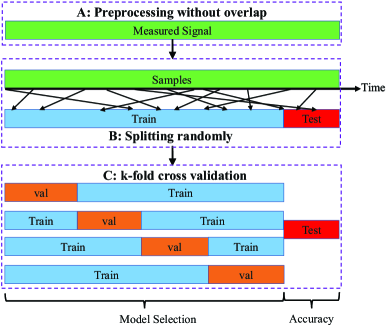
Figure 7: Random data splitting strategy with preprocessing without overlap.

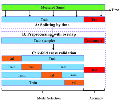
Figure 8: Another condition with the training and testing sets split as the first step.

For industrial data, they are rarely random and are always sequential (they might contain trends or other temporal correlation). Therefore, it is more appropriate to split data according to time sequences (order split). The diagram of data split strategy according to time sequences is shown in Fig. 9. From this diagram, it can be observed that we split the training and testing sets with the time phase instead of splitting the data randomly. In addition, Fig. 9 also shows the condition of 4-fold cross-validation with time. In the following study, we will compare the results of this strategy with the random split strategy.

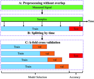
Figure 9: Data split according to time sequences.

8 Evaluation Methodology

8.1 Evaluation Metrics

It is a rather challenging task to evaluate the performance of intelligent diagnosis algorithms with suitable evaluation metrics. It has three standard evaluation metrics, which have been widely used, including the overall accuracy, the average accuracy, and the confusion matrix. In this paper, we only use the overall accuracy to evaluate the performance of algorithms. The overall accuracy is defined as the number of correctly classified samples divided by the total number of samples. The average accuracy is defined as the average classification accuracy of each category.

Since the performance of DL-based intelligent diagnosis algorithms fluctuates during the training process, to obtain reliable results and show the best overall accuracy that the model can achieve, we repeat each experiment five times. Four indicators are used to assess the performance of models, including the mean and maximum values of the overall accuracy obtained by the last epoch (the accuracy in the last epoch can represent the real accuracy without any test leakage), and the mean and maximum values of the maximal overall accuracy. For simplicity, they can be denoted as Last-Mean, Last-Max, Best-Mean, and Best-Max.

8.2 Experimental Setting

In the preparation stage, we use two strategies, including random split and order split to divide the dataset into training and testing sets. For random split, a sliding window is used to truncate the vibration signal without any overlap and each data sample contains 1024 points. After the preparation, we randomly take 80% of samples as the training set and 20% of samples as the testing set. For order split, we take the former 80% of time series as the training set and the last 20% as the testing set. Then, in two time series, a sliding window is used to truncate the vibration signal without any overlap, and each sample contains 1024 points.

In order to verify how input types, data normalization methods, and data split methods affect the performance of models, we set up three configurations of experiments (shown in Table 8, Table 9, and Table 10.). During model training, we use Adam as the optimizer. The learning rate and the batch size of each experiment are set to 0.001 and 64, respectively. Each model is trained for 100 epochs, and during the training procedure, model training and model testing are alternated. In addition, all the experiments are executed under Windows 10 and Pytorch 1.1 through running on a computer with an Intel Core i7-9700K, GeForce RTX 2080Ti, and 16G RAM.

Table 8: Experiment setup 1

Table 9: Experiment setup 2

Table 10: Experiment setup 3

9 Evaluation Results

In this section, we will first discuss the experimental results of different datasets in depth. After that, the results of datasets, input types, models, input normalization, data augmentation, and data splitting will be summarized separately. Complete results are shown in Appendix A. and each accuracy which is larger than 95% are bold.

9.1 Detailed Analysis of Different Datasets

A. CWRU Dataset

The results of CWRU dataset are shown in Appendix A from Table 1 to Table 3. From those results, we can observe that the accuracy of CNN models is generally higher than that of AE models. In addition, using FFT and STFT to process the signal allows models to achieve better accuracy among five kinds of input. CNN models with Z-score normalization can get better accuracy while using -1-1 normalization allows AE models to achieve higher accuracy. Using data augmentation does not improve the accuracy of AE models, but it can improve the accuracy of CNN models. The order split would slightly reduce the accuracy.

B. JNU Dataset

The results of JNU dataset are shown in Appendix A from Table 4 to Table 6. As can be seen from those tables, using FFT to process the raw signal allows models to achieve better accuracy among five types of input. CNN models with Z-score normalization can get better accuracy while using -1-1 normalization enables AE models to achieve higher accuracy. Using data augmentation can improve the accuracy of CNN models and AE models. The order split would highly reduce the accuracy.

C. MFPT Dataset

The results of MFPT dataset are shown in Appendix A from Table 7 to Table 9. We can observe that models with time or wavelet domain as the input would have the worse performance. However, using FFT to process the signal allows models to achieve better accuracy, and the accuracy of AE models is even higher than CNN models in this dataset. CNN models with Z-score normalization can get better accuracy while using -1-1 normalization enables the AE models to achieve higher accuracy. Using data augmentation can improve the accuracy of CNN models and AE models. The order split would heavily reduce the accuracy.

D. PU Dataset

The results of PU dataset are shown in Appendix A from Table 10 to Table 12. It is shown that the accuracy of CNN models is generally higher than that of AE models. Besides, the accuracy is worse when using the wavelet domain as the input, while using FFT and STFT to process the signal allows models to achieve better accuracy. Using Z-score normalization enables AE models and CNN models to achieve higher accuracy. Data augmentation does not help AE models improve the accuracy, while it can increase the accuracy of CNN models. Similarly, the order split would heavily reduce the accuracy.

E. SEU Dataset

The results of SEU dataset are shown in Appendix A from Table 13 to Table 15. We can observe that when using the time domain or wavelet domain as the input, models would achieve worse accuracy. However, using FFT to process the signal allows models to achieve better accuracy and the accuracy of AE models is even higher than that of CNN models. Using Z-score normalization allows AE models and CNN models to achieve higher accuracy. Data augmentation can improve the accuracy of both CNN and AE models. In this case, the order split would slightly reduce the accuracy.

F. UoC Dataset

The results of UoC dataset are shown in Appendix A from Table 16 to Table 18. We can observe that most models do not perform well in this case, and among them, the performance of AlexNet is relatively worse. Besides, using FFT to process the signal allows models to achieve bette accuracy, and the accuracy of AE models is higher than that of CNN models. AE models and CNN models with Z-score normalization would achieve higher accuracy. Data augmentation can help different models improve the final accuracy. The order split would heavily reduce the accuracy.

G. XJTU-SY Dataset

The results of XJTU-SY dataset are shown in Appendix A from Table 19 to Table 21. We can observe that most models perform well in this dataset. Besides, we can find that using FFT and STFT to process the signal allows models to achieve the better accuracy, and the accuracy of CNN models is higher than that of AE models, generally. AE models and CNN models with Z-score normalization would achieve higher accuracy. Data augmentation can help different models improve the final accuracy. The order split would quietly reduce the accuracy.

9.2 Results of Datasets

It can be seen from the results that with the exception of the UoC dataset, the accuracy of both AE and CNN models on those datasets exceeds 95%. In addition, the accuracy of CWRU, SEU and XJTU-SY datasets can reach to 100%. The accuracy of UoC is much lower than others in all conditions. Besides, the diagnostic difficulty of seven datasets can be ranked according to the number of diagnostic accuracy exceeding 95% in each dataset. As shown in Fig. 9, we can split the datasets into four levels of difficulty.

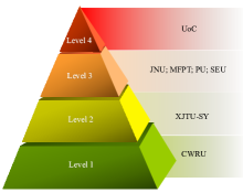
Figure 10: The level of dataset difficulty.

9.3 Results of Input Types

In all datasets, the frequency domain input can always achieve the highest accuracy followed by the time-frequency domain input since in the frequency domain, the noise is spread over the full frequency band and the fault information is much easier to be distinguished than that in the time domain. According to the computational load of CWT, we use the short length of samples to perform CWT and then upsample the wavelet coefficients. These steps may degrade the classification accuracy of CWT.

9.4 Results of Models

From the results, we can observe that models, especially ResNet18, can achieve the best accuracy in most of datasets including CWRU, JNU, PU, SEU, and XJTU-SY. However, for MFPT and UoC, models belonging to AE can perform better than other models. This phenomenon may be caused by the size of datasets and the overfitting problem. Therefore, not every dataset can get better results using a more complex model.

9.5 Results of Data Normalization

It is hard to conclude which data normalization method is the best one, and from the results, we can observe that the accuracy of different data normalization methods also depends on the used models and datasets. In general, Z-score normalization can make models achieve better accuracy.

9.6 Results of Data Augmentation

We can conclude that when the accuracy of datasets is already high enough, data augmentation methods may slightly degrade the performance because models have already fitted original datasets well. More augmentation methods may change the distribution of the original data and make the learning process harder. However, when the accuracy of datasets is not very high, data augmentation methods improve the performance of models, especially for the time domain input. Therefore, researchers can design other various data augmentation methods for their specific inputs.

9.7 Results of Data Splitting

When the datasets are easy to handle (CWRU and XJTU-SY), the results between random split and order split are quite similar. However, the accuracy of some datasets (PU and UoC) decreases sharply when using order split. What we should pay more attention to is that whether randomly splitting these datasets has the risk of test leakage. It may be more suitable for splitting the datasets according to time sequences to verify the performance.

According to the above discussion, we summarize the following conclusion coming from the evaluation results. First, not all datasets are suitable for comparing the classification effectiveness of the proposed methods since basic models can achieve very high accuracy on these datasets, like CWRU and XJTU-SY. Second, the frequency domain input can achieve the highest accuracy in all datasets, so researchers should first try to use the frequency domain as the input. Third, it is not necessary for CNN models to get the best results in all cases, and we also should consider the overfitting problem. Fourth, when the accuracy of datasets is not very high, data augmentation methods improve the performance of models, especially for the time domain input. Thus, more effective data augmentation methods need to be investigated. Finally, in some cases, it may be more suitable for splitting the datasets according to time sequences (order split) since random split may provide virtually high accuracy. We also release a code library to evaluate DL-based intelligent diagnosis algorithms and provide the benchmark accuracy (a lower bound) to avoid useless improvement. Meanwhile, we use specific-designed cases to discuss existing issues, including class imbalance, generalization ability, interpretability, few-shot learning, and model selection. Through these works, we aim to allow comparisons fairer and quicker, emphasize the importance of open source codes, and provide deep discussions of existing issues. To the best of our knowledge, this is the first work to comprehensively perform the benchmark study and release the code library to the public.

10 Discussion

Although intelligent diagnosis algorithms can achieve high classification accuracy in many datasets, there are still many issues that need to be discussed. In this paper, we further discuss the following five issues including class imbalance, generalization ability, interpretability, few-shot learning, and model selection using experimental cases.

10.1 Class Imbalance

Most of measured signals are in the normal state, and only a few of them are in the fault state, which means that fault modes often have different probabilities of happening. Therefore, the class imbalance issue will occur when using intelligent algorithms in real applications. Recently, although some researchers have published some related papers using traditional imbalanced learning methods [97] or GAN [98] to solve this problem, these studies are far from enough. In this paper, PU Bearing Datasets are used to simulate the class imbalance issue. In this experiment, we adopt ResNet18 as the experimental model and only use two kinds of input types (the time domain input and the frequency domain input). Besides, data augmentation methods are used and the normalization method is the Z-score normalization, while the dataset is randomly split. Three groups of datasets with different imbalance ratios are constructed, which are shown in Table 11.

Table 11: Number of samples in three groups of imbalanced datasets

Fault mode	Training samples			Testing samples
	Group1	Group2	Group3	Group1/2/3
KA04	125	125	125	125
KA15	125	75	50	125
KA16	125	75	50	125
KA22	125	75	50	125
KA30	125	37	25	125
KB23	125	37	25	125
KB24	125	37	25	125
KB27	125	25	6	125
KI14	125	25	6	125
KI16	125	25	6	125
KI17	125	12	2	125
KI18	125	12	2	125
KI21	125	12	2	125

As shown in Table 11, three datasets (Group1, Group2, and Group3) are constituted with different imbalanced ratios. Group1 is a balanced dataset, and there is no imbalance for each state. In real applications, it is almost impossible to let the number of data samples be the same. We reduce the training samples of some fault modes in Group1 to construct Group2, and then the imbalanced classification is simulated. In Group3, the imbalanced ratio between fault modes increases further. Group2 can be considered as a moderately imbalanced dataset, while Group3 can be considered as a highly imbalanced dataset.

Experimental results are shown in Fig. 11, and it can be observed that the overall accuracy in Group3 is much lower than that of Group1, which indicates that the class imbalance will greatly degrade the performance of models. To address the problem of class imbalance, data-level methods and classifier-level methods can be used [99]. Oversampling and undersampling methods are the most commonly used data-level methods, and some methods for generating samples based on GAN have also been studied recently. For the classifier-level methods, thresholding-based methods are applied in the test phase to adjust the decision threshold of the classifier. Besides, cost-sensitive learning methods assign different weights to different classes to avoid the suppression of categories with a small number of samples. In the field of intelligent diagnosis, other methods based on physical meanings and fault attention need to be explored.

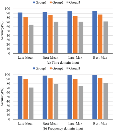
Figure 11: Experimental results of three groups of datasets. (a) time domain input, and (b) frequency domain input.

10.2 Generalization ability

Many existing intelligent algorithms perform very well on one working condition, but the diagnostic performance tends to drop significantly on another working condition, and here, we call it the generalization problem. Recently, many researchers have used algorithms based on transfer learning strategies to solve this problem, and a comparative study with open source codes was performed in [100]. To illustrate the weak generalization ability of the intelligent diagnosis algorithms, experiments are also carried out on the PU bearing dataset. Experiments use the data under three working conditions (N15_M07_F10, N09_M07_F10, N15_M01_F10). In these experiments, data under one working condition is used to train models, and data under another working condition is used to test the performance. A total of six groups are performed, and the detailed information is shown in Table 12.

Table 12: Training data and testing data for each experiment

Group	Data for training	Data for testing
Group1	N15_M07_F10	N09_M07_F10
Group2	N15_M07_F10	N15_M01_F10
Group3	N09_M07_F10	N15_M07_F10
Group4	N09_M07_F10	N15_M01_F10
Group5	N15_M01_F10	N15_M07_F10
Group6	N15_M01_F10	N09_M07_F10

The experimental results are shown in Fig. 12. It can be concluded that in most cases, intelligent diagnosis algorithms trained on one working condition cannot perform well on another working condition, which means the generalization ability of algorithms is insufficient. In general, we expect that our algorithms could adapt to the changes in working conditions or measurement situations since these changes occur frequently in real applications. Therefore, studies are still required on how to transfer the trained algorithms to different working conditions effectively.

Two excellent review papers [101, 102] and other applications [103, 104] published recently pointed out several potential research directions which could be considered and studied further to improve the generalization ability.

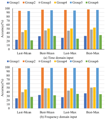
Figure 12: Experimental results of working conditions transfer. (a) time domain input, and (b) frequency domain input.

10.3 Interpretability

Although intelligent diagnosis algorithms can achieve high diagnostic accuracy in their tasks, the interpretability of these models is often insufficient and these black-box models would generate high-risk results [105], which greatly limits their applications. Actually, some papers in intelligent diagnosis have noted this problem and attempted to propose some interpretable models [106, 107].

To point out that intelligent diagnostic algorithms lack interpretability, we perform three sets of experiments on the PU bearing dataset, and the datasets are shown in Table 13. In each set of experiments, we use two different data, which have the same fault pattern and are acquired under the same condition.

Table 13: The bearing code and the number of samples used in each experiment

Group	Bearing code	Training samples	Testing samples
Group1	KA03	200	50
	KA06	200	50
Group2	KA08	200	50
	KA09	200	50
Group3	KI07	200	50
	KI08	200	50

The results, in which intelligent algorithms can get high accuracy in each set of experiments, are shown in Fig. 13. Nevertheless, for each binary classification task, since the fault mode and the working condition at the time of acquisition are the same between two classes, theoretically, methods should not be able to achieve such high accuracy. These expected results are exactly contrary to those of the experiment, which shows that models only learn the discrimination of different collection points and do not learn how to extract the essential characteristics of fault signals. Therefore, it is very important to figure out whether models can learn essential fault characteristics or just classify the different conditions of collected signals.

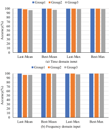
Figure 13: Experimental results of three groups. (a) time domain input, and (b) frequency domain input.

According to the development of interpretability, we might be able to study the interpretability of DL-based models from the following aspects: (1) visualize the results of neurons to analyze the attention points of models [108]; (2) add physical constraints to the loss function [109] to meet specific needs of fault feature extraction; (3) add prior knowledge to network structures and convolutions [110] or unroll the existing optimization algorithms [111] to extract corresponding fault features.

10.4 Few-Shot Learning

In intelligent diagnosis, the amount of data is far from big data because of the preciousness of fault data and the high cost of fault simulation experiments, especially for the key components. To manifest the influence of the sample number on the classification accuracy, we use the PU bearing dataset to design a few-shot training pattern with six groups of different sample numbers in each class.

Results of the time domain input and the frequency domain input are shown in Fig. 14. It is shown that with the decrease of the sample number, the accuracy decreases sharply. As shown in Fig. 14, for the time domain input, the Best-Max accuracy decreases from 91.46% to 20.39% as the sample number decreases from 100 to 1. Meanwhile, the Best-Max accuracy decreases from 97.73% to 29.67% as the sample number decreases from 100 to 1 with the frequency domain input.

Although the accuracy can be increased after using FFT, it is still too low to be accepted when the number of samples is extremely small. It is necessary to develop methods based on few-shot learning to cope with application scenarios with limited samples.

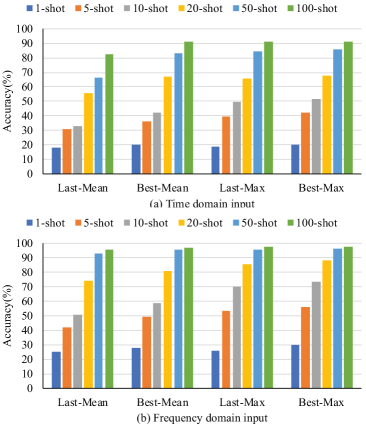
Figure 14: Experimental results of different few-shot training patterns. (a) time domain input, and (b) frequency domain input.

Many DL-based few-shot learning models have been proposed in recent years [112], most of these methods adopt a meta-learning paradigm by training networks with a large number of tasks, which means that the big data in other related fields is necessary for these methods. In the field of fault diagnosis, there is no relevant data with such a big size available, so methods embedding with physical mechanisms are required to address this problem effectively.

10.5 Model selection

For intelligent diagnosis, designing a neural network is not the final goal, and our task is to apply the model to real industrial applications while designing a neural network is only a small part of our task. However, to achieve a good effect, we have to spend considerable time and energy on designing the corresponding networks. Because building a neural network is an iterative process consisting of repeated trial and error, and the performance of models should be fed back to us to adjust models. The single trial and error cost multiplied by the number of trial and error can easily reach a huge cost. Besides, reducing this cost is also the partial purpose of this benchmark study which provides some guidelines to choose a baseline model.

Actually, there is another way called neural architecture search (NAS) [113] to avoid the huge cost of trial and error. NAS can allow designing a neural network automatically through searching for a specific network based on a specific dataset. Limited search space of the network is first constructed according to the physical prior. After that, a neural network matching a specific dataset is sampled from the search space through reinforcement learning, the evolutionary algorithm or the gradient strategy. Besides, the whole construction process does not require manual participation, which greatly reduces the cost of building a neural network and allows us to focus on specific engineering applications.

11 Conclusion

In this paper, we collect nine publicly available datasets to evaluate the performance of MLP, AE, CNN, and RNN models. This work mainly focuses on evaluating DL-based intelligent diagnosis algorithms from different perspectives and providing the benchmark accuracy (a lower bound) to avoid useless improvement. In addition, we release a code library for other researchers to test the performance of their own DL-based intelligent diagnosis models of these datasets. We hope that the evaluation results and the code library could promote a better understanding of DL-based models and provide a unified framework for generating more effective models. For further studies, we will focus on five listed issues (class imbalance, generalization ability, interpretability, few-shot learning, and model selection) to propose more customized works.

See pages 1-21 of Figs/Results.pdf

References

- Zhao et al. [2018] Z. Zhao, S. Wu, B. Qiao, S. Wang, X. Chen, Enhanced sparse period-group lasso for bearing fault diagnosis, IEEE Transactions on Industrial Electronics 66 (2018) 2143–2153.
- Wang et al. [2016] S. Wang, X. Chen, C. Tong, Z. Zhao, Matching synchrosqueezing wavelet transform and application to aeroengine vibration monitoring, IEEE Transactions on Instrumentation and Measurement 66 (2016) 360–372.
- Sun et al. [2018] C. Sun, M. Ma, Z. Zhao, X. Chen, Sparse deep stacking network for fault diagnosis of motor, IEEE Transactions on Industrial Informatics 14 (2018) 3261–3270.
- Krizhevsky et al. [2012] A. Krizhevsky, I. Sutskever, G. E. Hinton, Imagenet classification with deep convolutional neural networks, in: Advances in neural information processing systems, pp. 1097–1105.
- Farabet et al. [2012] C. Farabet, C. Couprie, L. Najman, Y. LeCun, Learning hierarchical features for scene labeling, IEEE transactions on pattern analysis and machine intelligence 35 (2012) 1915–1929.
- Hirschberg and Manning [2015] J. Hirschberg, C. D. Manning, Advances in natural language processing, Science 349 (2015) 261–266.
- Sun et al. [2017] S. Sun, C. Luo, J. Chen, A review of natural language processing techniques for opinion mining systems, Information fusion 36 (2017) 10–25.
- Young et al. [2018] T. Young, D. Hazarika, S. Poria, E. Cambria, Recent trends in deep learning based natural language processing, ieee Computational intelligenCe magazine 13 (2018) 55–75.
- Feng et al. [2019] Q. Feng, X. Zhao, D. Fan, B. Cai, Y. Liu, Y. Ren, Resilience design method based on meta-structure: A case study of offshore wind farm, Reliability Engineering & System Safety 186 (2019) 232–244.
- Li et al. [2020] D. Li, Y. Liu, D. Huang, Development of semi-supervised multiple-output soft-sensors with co-training and tri-training mpls and mrvm, Chemometrics and Intelligent Laboratory Systems 199 (2020) 103970.
- Hinton and Salakhutdinov [2006] G. E. Hinton, R. R. Salakhutdinov, Reducing the dimensionality of data with neural networks, science 313 (2006) 504–507.
- MIT Technology Review [2019] MIT Technology Review, 10 Breakthrough Technologies 2013, https://www.technologyreview.com/lists/technologies/2013/, accessed on August 2019.
- LeCun et al. [2015] Y. LeCun, Y. Bengio, G. Hinton, Deep learning, nature 521 (2015) 436.
- Riley [2019] P. Riley, Three pitfalls to avoid in machine learning, 2019.
- Goodfellow et al. [2016] I. Goodfellow, Y. Bengio, A. Courville, Deep learning, MIT press, 2016.
- Li et al. [2018] C. Li, J. L. V. de Oliveira, M. C. Lozada, D. Cabrera, V. Sanchez, G. Zurita, A systematic review of fuzzy formalisms for bearing fault diagnosis, IEEE Transactions on Fuzzy Systems (2018).
- Hoang and Kang [2019] D.-T. Hoang, H.-J. Kang, A survey on deep learning based bearing fault diagnosis, Neurocomputing 335 (2019) 327–335.
- Zhang et al. [2020] S. Zhang, S. Zhang, B. Wang, T. G. Habetler, Deep learning algorithms for bearing fault diagnosticsx-a comprehensive review, IEEE Access 8 (2020) 29857–29881.
- Hamadache et al. [2019] M. Hamadache, J. H. Jung, J. Park, B. D. Youn, A comprehensive review of artificial intelligence-based approaches for rolling element bearing phm: shallow and deep learning, JMST Advances 1 (2019) 125–151.
- Ali et al. [2016] Y. H. Ali, S. M. Ali, R. A. Rahman, R. I. R. Hamzah, Acoustic emission and artificial intelligent methods in condition monitoring of rotating machine–a review, in: National Conference For Postgraduate Research (NCON-PGR 2016).
- Liu et al. [2018] R. Liu, B. Yang, E. Zio, X. Chen, Artificial intelligence for fault diagnosis of rotating machinery: A review, Mechanical Systems and Signal Processing 108 (2018) 33–47.
- Wei et al. [2019] Y. Wei, Y. Li, M. Xu, W. Huang, A review of early fault diagnosis approaches and their applications in rotating machinery, Entropy 21 (2019) 409.
- Zhao et al. [2016] G. Zhao, G. Zhang, Q. Ge, X. Liu, Research advances in fault diagnosis and prognostic based on deep learning, in: 2016 Prognostics and System Health Management Conference (PHM-Chengdu), IEEE, pp. 1–6.
- Duan et al. [2018] L. Duan, M. Xie, J. Wang, T. Bai, Deep learning enabled intelligent fault diagnosis: Overview and applications, Journal of Intelligent & Fuzzy Systems 35 (2018) 5771–5784.
- Zhang et al. [2017] W. Zhang, M.-P. Jia, L. Zhu, X.-A. Yan, Comprehensive overview on computational intelligence techniques for machinery condition monitoring and fault diagnosis, Chinese Journal of Mechanical Engineering 30 (2017) 782–795.
- Zhao et al. [2019] R. Zhao, R. Yan, Z. Chen, K. Mao, P. Wang, R. X. Gao, Deep learning and its applications to machine health monitoring, Mechanical Systems and Signal Processing 115 (2019) 213–237.
- Lei et al. [2020] Y. Lei, B. Yang, X. Jiang, F. Jia, N. Li, A. K. Nandi, Applications of machine learning to machine fault diagnosis: A review and roadmap, Mechanical Systems and Signal Processing 138 (2020) 106587.
- Nasiri et al. [2017] S. Nasiri, M. R. Khosravani, K. Weinberg, Fracture mechanics and mechanical fault detection by artificial intelligence methods: A review, Engineering Failure Analysis 81 (2017) 270–293.
- Tian et al. [2018] Y. Tian, D. Guo, K. Zhang, L. Jia, H. Qiao, H. Tang, A review of fault diagnosis for traction induction motor, in: 2018 37th Chinese Control Conference (CCC), IEEE, pp. 5763–5768.
- Khan and Yairi [2018] S. Khan, T. Yairi, A review on the application of deep learning in system health management, Mechanical Systems and Signal Processing 107 (2018) 241–265.
- Stetco et al. [2018] A. Stetco, F. Dinmohammadi, X. Zhao, V. Robu, D. Flynn, M. Barnes, J. Keane, G. Nenadic, Machine learning methods for wind turbine condition monitoring: A review, Renewable energy (2018).
- Ellefsen et al. [2019] A. L. Ellefsen, V. Æsøy, S. Ushakov, H. Zhang, A comprehensive survey of prognostics and health management based on deep learning for autonomous ships, IEEE Transactions on Reliability 68 (2019) 720–740.
- Ademujimi et al. [2017] T. T. Ademujimi, M. P. Brundage, V. V. Prabhu, A review of current machine learning techniques used in manufacturing diagnosis, in: IFIP International Conference on Advances in Production Management Systems, Springer, pp. 407–415.
- Chang et al. [2018] C.-W. Chang, H.-W. Lee, C.-H. Liu, A review of artificial intelligence algorithms used for smart machine tools, Inventions 3 (2018) 41.
- Wang et al. [2018] J. Wang, Y. Ma, L. Zhang, R. X. Gao, D. Wu, Deep learning for smart manufacturing: Methods and applications, Journal of Manufacturing Systems 48 (2018) 144–156.
- Sharp et al. [2018] M. Sharp, R. Ak, T. Hedberg Jr, A survey of the advancing use and development of machine learning in smart manufacturing, Journal of manufacturing systems 48 (2018) 170–179.
- Mao et al. [2020] W. Mao, J. Chen, X. Liang, X. Zhang, A New Online Detection Approach for Rolling Bearing Incipient Fault via Self-Adaptive Deep Feature Matching, IEEE Transactions on Instrumentation and Measurement 69 (2020) 443–456.
- Chen et al. [2020] L. Chen, Z. Zhang, J. Cao, X. Wang, A novel method of combining nonlinear frequency spectrum and deep learning for complex system fault diagnosis, Measurement 151 (2020).
- Zhang et al. [2020] Y. Zhang, X. Li, L. Gao, W. Chen, P. Li, Intelligent fault diagnosis of rotating machinery using a new ensemble deep auto-encoder method, Measurement 151 (2020).
- Kong et al. [2020] X. Kong, G. Mao, Q. Wang, H. Ma, W. Yang, A multi-ensemble method based on deep auto-encoders for fault diagnosis of rolling bearings, Measurement 151 (2020).
- Jiang et al. [2020] N. Jiang, X. Hu, N. Li, Graphical temporal semi-supervised deep learning-based principal fault localization in wind turbine systems, Proceedings of the Institution of Mechanical Engineers, Part I: Journal of Systems and Control Engineering (2020).
- Li et al. [2020] X. Li, J. Li, Y. Qu, D. He, Semi-supervised gear fault diagnosis using raw vibration signal based on deep learning, Chinese Journal of Aeronautics 33 (2020) 418–426.
- Xiong et al. [2020] X. Xiong, H. Jiang, X. Li, M. Niu, A Wasserstein gradient-penalty generative adversarial network with deep auto-encoder for bearing intelligent fault diagnosis, Measurement Science and Technology 31 (2020).
- Zhou et al. [2020] F. Zhou, S. Yang, H. Fujita, D. Chen, C. Wen, Deep learning fault diagnosis method based on global optimization GAN for unbalanced data, Knowledge-Based Systems 187 (2020).
- Guo et al. [2020] Q. Guo, Y. Li, Y. Song, D. Wang, W. Chen, Intelligent Fault Diagnosis Method Based on Full 1-D Convolutional Generative Adversarial Network, IEEE Transactions on Industrial Informatics 16 (2020) 2044–2053.
- Zhao et al. [2020] X. Zhao, M. Jia, M. Lin, Deep Laplacian Auto-encoder and its application into imbalanced fault diagnosis of rotating machinery, Measurement 152 (2020).
- Zhiyi et al. [2020a] H. Zhiyi, S. Haidong, J. Lin, C. Junsheng, Y. Yu, Transfer fault diagnosis of bearing installed in different machines using enhanced deep auto-encoder, Measurement 152 (2020a).
- Zhiyi et al. [2020b] H. Zhiyi, S. Haidong, W. Ping, J. J. Lin, C. Junsheng, Y. Yu, Deep transfer multi-wavelet auto-encoder for intelligent fault diagnosis of gearbox with few target training samples, Knowledge-Based Systems 191 (2020b).
- Li et al. [2020] X. Li, X.-D. Jia, W. Zhang, H. Ma, Z. Luo, X. Li, Intelligent cross-machine fault diagnosis approach with deep auto-encoder and domain adaptation, Neurocomputing 383 (2020) 235–247.
- Mao et al. [2020] W. Mao, D. Zhang, S. Tian, J. Tang, Robust Detection of Bearing Early Fault Based on Deep Transfer Learning, Electronics 9 (2020).
- Zhang et al. [2020] Y. Zhang, K. Xing, R. Bai, D. Sun, Z. Meng, An enhanced convolutional neural network for bearing fault diagnosis based on time-frequency image, Measurement 157 (2020).
- Khodja et al. [2020] A. Y. Khodja, N. Guersi, M. N. Saadi, N. Boutasseta, Rolling element bearing fault diagnosis for rotating machinery using vibration spectrum imaging and convolutional neural networks, The International Journal of Advanced Manufacturing Technology 106 (2020) 1737–1751.
- Li et al. [2020] Y. Li, X. Du, F. Wan, X. Wang, H. Yu, Rotating machinery fault diagnosis based on convolutional neural network and infrared thermal imaging, Chinese Journal of Aeronautics 33 (2020) 427–438.
- Zhang et al. [2020] J. Zhang, Y. Sun, L. Guo, H. Gao, X. Hong, H. Song, A new bearing fault diagnosis method based on modified convolutional neural networks, Chinese Journal of Aeronautics 33 (2020) 439–447.
- Zhao et al. [2020] M. Zhao, B. Tang, L. Deng, M. Pecht, Multiple wavelet regularized deep residual networks for fault diagnosis, Measurement 152 (2020).
- Li et al. [2020] X. Li, W. Zhang, Q. Ding, J.-Q. Sun, Intelligent rotating machinery fault diagnosis based on deep learning using data augmentation, Journal of Intelligent Manufacturing 31 (2020) 433–452.
- Tang et al. [2020] T. Tang, T. Hu, M. Chen, R. Lin, G. Chen, A deep convolutional neural network approach with information fusion for bearing fault diagnosis under different working conditions, Proceedings of the Institution of Mechanical Engineers, Part C: Journal of Mechanical Engineering Science (2020).
- Xue et al. [2020] Y. Xue, D. Dou, J. Yang, Multi-fault diagnosis of rotating machinery based on deep convolution neural network and support vector machine, Measurement 156 (2020).
- Verstraete et al. [2020] D. B. Verstraete, E. Lopez Droguett, V. Meruane, M. Modarres, A. Ferrada, Deep semi-supervised generative adversarial fault diagnostics of rolling element bearings, Structural Health Monitoring 19 (2020) 390–411.
- Zhang et al. [2020] W. Zhang, X. Li, X.-D. Jia, H. Ma, Z. Luo, X. Li, Machinery fault diagnosis with imbalanced data using deep generative adversarial networks, Measurement 152 (2020).
- Li et al. [2020] T. Li, Z. Zhao, C. Sun, R. Yan, X. Chen, Adaptive channel weighted cnn with multi-sensor fusion for condition monitoring of helicopter transmission system, IEEE Sensors Journal (2020).
- Xu et al. [2020] G. Xu, M. Liu, Z. Jiang, W. Shen, C. Huang, Online Fault Diagnosis Method Based on Transfer Convolutional Neural Networks, IEEE Transactions on Instrumentation and Measurement 69 (2020) 509–520.
- Mao et al. [2020] W. Mao, L. Ding, S. Tian, X. Liang, Online detection for bearing incipient fault based on deep transfer learning, Measurement 152 (2020).
- Chen et al. [2020] Z. Chen, K. Gryllias, W. Li, Intelligent Fault Diagnosis for Rotary Machinery Using Transferable Convolutional Neural Network, IEEE Transactions on Industrial Informatics 16 (2020) 339–349.
- Li et al. [2020] Q. Li, B. Tang, L. Deng, Y. Wu, Y. Wang, Deep balanced domain adaptation neural networks for fault diagnosis of planetary gearboxes with limited labeled data, Measurement 156 (2020).
- Jiao et al. [2019] J. Jiao, M. Zhao, J. Lin, Unsupervised adversarial adaptation network for intelligent fault diagnosis, IEEE Transactions on Industrial Electronics (2019).
- Grezmak et al. [2020] J. Grezmak, J. Zhang, P. Wang, K. A. Loparo, R. X. Gao, Interpretable Convolutional Neural Network Through Layer-wise Relevance Propagation for Machine Fault Diagnosis, IEEE Sensors Journal 20 (2020) 3172–3181.
- Haidong et al. [2020] S. Haidong, C. Junsheng, J. Hongkai, Y. Yu, W. Zhantao, Enhanced deep gated recurrent unit and complex wavelet packet energy moment entropy for early fault prognosis of bearing, Knowledge-Based Systems 188 (2020).
- Zhao et al. [2020] K. Zhao, H. Jiang, X. Li, R. Wang, An optimal deep sparse autoencoder with gated recurrent unit for rolling bearing fault diagnosis, Measurement Science and Technology 31 (2020).
- Wu et al. [2020] Z. Wu, H. Jiang, K. Zhao, X. Li, An adaptive deep transfer learning method for bearing fault diagnosis, Measurement 151 (2020).
- Ma et al. [2020] Y. Ma, X. Jia, H. Bai, G. Wang, G. Liu, C. Guo, A new fault diagnosis method using deep belief network and compressive sensing, Journal of Vibroengineering 22 (2020) 83–97.
- Yan et al. [2020] L.-P. Yan, X.-Z. Dong, T. Wang, Q. Gao, C.-Q. Tan, D.-T. Zeng, H.-l. Zhang, H.-s. Chen, A fault diagnosis method for gas turbines based on improved data preprocessing and an optimization deep belief network, Measurement Science and Technology 31 (2020).
- Yu et al. [2020] K. Yu, T. R. Lin, J. Tan, A bearing fault and severity diagnostic technique using adaptive deep belief networks and Dempster-Shafer theory, Structural Health Monitoring 19 (2020) 240–261.
- Ding et al. [2019] Y. Ding, L. Ma, J. Ma, M. Suo, L. Tao, Y. Cheng, C. Lu, Intelligent fault diagnosis for rotating machinery using deep q-network based health state classification: A deep reinforcement learning approach, Advanced Engineering Informatics 42 (2019) 100977.
- Dai et al. [2020] W. Dai, Z. Mo, C. Luo, J. Jiang, H. Zhang, Q. Miao, Fault diagnosis of rotating machinery based on deep reinforcement learning and reciprocal of smoothness index, IEEE Sensors Journal (2020).
- Zhang et al. [2020] D. Zhang, E. Stewart, M. Entezami, C. Roberts, D. Yu, Intelligent acoustic-based fault diagnosis of roller bearings using a deep graph convolutional network, Measurement 156 (2020).
- Rumelhart et al. [1985] D. E. Rumelhart, G. E. Hinton, R. J. Williams, Learning internal representations by error propagation, Technical Report, California Univ San Diego La Jolla Inst for Cognitive Science, 1985.
- Vincent et al. [2008] P. Vincent, H. Larochelle, Y. Bengio, P.-A. Manzagol, Extracting and composing robust features with denoising autoencoders, in: Proceedings of the 25th international conference on Machine learning, ACM, pp. 1096–1103.
- Ranzato et al. [2007] M. Ranzato, C. Poultney, S. Chopra, Y. L. Cun, Efficient learning of sparse representations with an energy-based model, in: Advances in neural information processing systems, pp. 1137–1144.
- LeCun and Bengio [1995] Y. LeCun, Y. Bengio, Convolutional networks for images, speech, and time series, The handbook of brain theory and neural networks 3361 (1995) 1995.
- He et al. [2016] K. He, X. Zhang, S. Ren, J. Sun, Deep residual learning for image recognition, in: Proceedings of the IEEE conference on computer vision and pattern recognition, pp. 770–778.
- Hochreiter and Schmidhuber [1997] S. Hochreiter, J. Schmidhuber, Long short-term memory, Neural computation 9 (1997) 1735–1780.
- CWR [mber] Case Western Reserve University (CWRU) Bearing Data Center, [Online], Available: https://csegroups.case.edu/bearingdatacenter/pages/download-data-file/, Accessed 2019, September.
- MFP [mber] Society For Machinery Failure Prevention Technology, [Online], Available: https://mfpt.org/fault-data-sets/, Accessed 2019, September.
- Lessmeier et al. [2019] C. Lessmeier, J. K. Kimotho, D. Zimmer, W. Sextro, KAt-DataCenter, Chair of Design and Drive Technology, Paderborn University, https://mb.uni-paderborn.de/kat/forschung/datacenter/bearing-datacenter/, accessed on August 2019.
- Lessmeier et al. [2016] C. Lessmeier, J. K. Kimotho, D. Zimmer, W. Sextro, Condition monitoring of bearing damage in electromechanical drive systems by using motor current signals of electric motors: A benchmark data set for data-driven classification, in: Proceedings of the European conference of the prognostics and health management society, pp. 05–08.
- Cao et al. [mber] P. Cao, S. Zhang, J. Tang, Gear Fault Data, [Online], Available: https://doi.org/10.6084/m9.figshare.6127874.v1, Accessed 2019, September.
- XJT [mber] XJTU-SY Bearing Datasets, [Online], Available: http://biaowang.tech/xjtu-sy-bearing-datasets/, Accessed 2019, September.
- Wang et al. [2018] B. Wang, Y. Lei, N. Li, N. Li, A hybrid prognostics approach for estimating remaining useful life of rolling element bearings, IEEE Transactions on Reliability (2018).
- SEU [mber] SEU gearbox datasets, [Online], Available: https://github.com/cathysiyu/Mechanical-datasets, Accessed 2019, September.
- Shao et al. [2018] S. Shao, S. McAleer, R. Yan, P. Baldi, Highly accurate machine fault diagnosis using deep transfer learning, IEEE Transactions on Industrial Informatics 15 (2018) 2446–2455.
- Li [2019] K. Li, School of Mechanical Engineering, Jiangnan University, http://mad-net.org:8765/explore.html?t=0.5831516555847212., accessed on August 2019.
- Li et al. [2013] K. Li, X. Ping, H. Wang, P. Chen, Y. Cao, Sequential fuzzy diagnosis method for motor roller bearing in variable operating conditions based on vibration analysis, Sensors 13 (2013) 8013–8041.
- PHM [mber] PHM IEEE 2012 Data Challenge, [Online], Available: https://github.com/wkzs111/phm-ieee-2012-data-challenge-dataset, Accessed 2019, September.
- Nectoux et al. [2012] P. Nectoux, R. Gouriveau, K. Medjaher, E. Ramasso, B. Chebel-Morello, N. Zerhouni, C. Varnier, Pronostia: An experimental platform for bearings accelerated degradation tests., in: IEEE International Conference on Prognostics and Health Management, PHM’12., IEEE Catalog Number: CPF12PHM-CDR, pp. 1–8.
- Lee et al. [2007] J. Lee, H. Qiu, G. Yu, J. a. Lin, Bearing data set, IMS, University of Cincinnati, NASA Ames Prognostics Data Repository, (https://ti.arc.nasa.gov/tech/dash/groups/pcoe/prognostic-data-repository/), NASA Ames Research Center, Moffett Field, CA (2007).
- Zhang et al. [2018] Y. Zhang, X. Li, L. Gao, L. Wang, L. Wen, Imbalanced data fault diagnosis of rotating machinery using synthetic oversampling and feature learning, Journal of manufacturing systems 48 (2018) 34–50.
- Mao et al. [2019] W. Mao, Y. Liu, L. Ding, Y. Li, Imbalanced fault diagnosis of rolling bearing based on generative adversarial network: A comparative study, IEEE Access 7 (2019) 9515–9530.
- Buda et al. [2018] M. Buda, A. Maki, M. A. Mazurowski, A systematic study of the class imbalance problem in convolutional neural networks, Neural Networks 106 (2018) 249–259.
- Zhao et al. [2019] Z. Zhao, Q. Zhang, X. Yu, C. Sun, S. Wang, R. Yan, X. Chen, Unsupervised deep transfer learning for intelligent fault diagnosis: An open source and comparative study, arXiv preprint arXiv:1912.12528 (2019).
- Zheng et al. [2019] H. Zheng, R. Wang, Y. Yang, J. Yin, Y. Li, Y. Li, M. Xu, Cross-domain fault diagnosis using knowledge transfer strategy: a review, IEEE Access 7 (2019) 129260–129290.
- Yan et al. [2019] R. Yan, F. Shen, C. Sun, X. Chen, Knowledge transfer for rotary machine fault diagnosis, IEEE Sensors Journal (2019).
- Han et al. [2019a] T. Han, C. Liu, W. Yang, D. Jiang, Deep transfer network with joint distribution adaptation: A new intelligent fault diagnosis framework for industry application, ISA transactions (2019a).
- Han et al. [2019b] T. Han, C. Liu, W. Yang, D. Jiang, Learning transferable features in deep convolutional neural networks for diagnosing unseen machine conditions, ISA transactions 93 (2019b) 341–353.
- Rudin [2019] C. Rudin, Stop explaining black box machine learning models for high stakes decisions and use interpretable models instead, Nature Machine Intelligence 1 (2019) 206–215.
- Li et al. [2019a] X. Li, W. Zhang, Q. Ding, Understanding and improving deep learning-based rolling bearing fault diagnosis with attention mechanism, Signal Processing 161 (2019a) 136–154.
- Li et al. [2019b] T. Li, Z. Zhao, C. Sun, L. Cheng, X. Chen, R. Yan, R. X. Gao, Waveletkernelnet: An interpretable deep neural network for industrial intelligent diagnosis, arXiv preprint arXiv:1911.07925 (2019b).
- Zeiler and Fergus [2014] M. D. Zeiler, R. Fergus, Visualizing and understanding convolutional networks, in: European conference on computer vision, Springer, pp. 818–833.
- Tang et al. [2018] M. Tang, F. Perazzi, A. Djelouah, I. Ben Ayed, C. Schroers, Y. Boykov, On regularized losses for weakly-supervised cnn segmentation, in: Proceedings of the European Conference on Computer Vision (ECCV), pp. 507–522.
- Ravanelli and Bengio [2018] M. Ravanelli, Y. Bengio, Interpretable convolutional filters with sincnet, arXiv preprint arXiv:1811.09725 (2018).
- Gregor and LeCun [2010] K. Gregor, Y. LeCun, Learning fast approximations of sparse coding, in: Proceedings of the 27th International Conference on International Conference on Machine Learning, Omnipress, pp. 399–406.
- Wang et al. [2019] Y. Wang, Q. Yao, J. Kwok, L. M. Ni, Generalizing from a few examples: A survey on few-shot learning, in: arXiv: 1904.05046, 2019.
- Elsken et al. [2019] T. Elsken, J. H. Metzen, F. Hutter, Neural architecture search: A survey., Journal of Machine Learning Research 20 (2019) 1–21.