Multiplex Recurrence Networks

Abstract

We have introduced a novel multiplex recurrence network (MRN) approach by combining recurrence networks with the multiplex network approach in order to investigate multivariate time series. The potential use of this approach is demonstrated on coupled map lattices and a typical example from palaeobotany research. In both examples, topological changes in the multiplex recurrence networks allow for the detection of regime changes in their dynamics. The method goes beyond classical interpretation of pollen records by considering the vegetation as a whole and using the intrinsic similarity in the dynamics of the different regional vegetation elements. We find that the different vegetation types behave more similar when one environmental factor acts as the dominant driving force.

I Introduction

In order to understand the dynamical behavior of systems in a broad range of scientific fields such as physics, biology, medicine, climatology, economy etc., time series analysis provides crucial techniques. Although investigation of time series can be done by various techniques, such as basic statistics, symbolization, power spectra or similarity analysis, phase space based methods have become an important role in dynamical systems’ analysis. Recurrence of a trajectory in its phase space is one of the most important fundamental features of dynamical systems. Related approaches have been used for several decades. The first recurrence based approach is known as the Poincaré recurrence theorem introduced in 1890 Poincaré (1890). The theorem indicates that almost all trajectories of dynamical systems will turn back infinitesimally close to their previous positions after a sufficiently long but finite time Poincaré (1890). Continuous dynamical systems can be defined by a set of ordinary differential equations. These equation sets are called as flows and if the phase space of a flow has a bounded volume, then the Poincaré recurrence theorem is always valid Katok and Hasselblatt (1995). Among the many different approaches of analyzing dynamical systems by their recurrence, the recurrence plot (RP) is a multifaceted and powerful approach to study different aspects of dynamical systems. Introduced by Eckmann et al. in 1987, the RP is a matrix to show the times of recurrences of a trajectory in its phase space Eckmann et al. (1987). Afterwards, many statistical quantification methods based on RP were developed for characterizing dynamical properties, regime transitions, synchronization, etc. Marwan et al. (2007).

Understanding underlying dynamics and detecting possible regime changes in the evolution of dynamical systems are important problems studied by time series analysis. For instance, we assume a dynamical system

$$\vec{\dot{x}}=f(\vec{x},r)$$ (1)

where $\vec{x}\in\mathbb{R}^{m}$, $f:\mathbb{R}^{m}\to\mathbb{R}^{m}$ and a control parameter ($r$) that has not to be constant on time $r=g(t)$. The purpose of the analysis is to detect possible dynamical regime changes in the time series caused by the time dependence of $r$. Transitions in the dynamics can be detected by different RP based measures, which in general are powerful to study complex, real-world systems Trulla et al. (1996); Marwan et al. (2002); Donges et al. (2011). Examples of their successful application to real-world systems have been found in medicine Jansen (1991); Kaplan et al. (1991); Riley et al. (1999); Marwan et al. (2002); Neuman et al. (2009); Carrubba et al. (2012), Earth science Richards (1994); Marwan et al. (2003); Matcharashvili et al. (2008); Donges et al. (2011); Ozken et al. (2015); Eroglu et al. (2016), astrophysics Asghari et al. (2004); Zolotova et al. (2009), electrochemistry  Eroglu et al. (2014a), and others Marwan (2008); Grassberger and Procaccia (1983a, 1984).

In the last decade, transformation of a time series to a complex network has become a very powerful approach to analyze complex dynamical systems. There are several ways to convert a time series to a network such as symbolic dynamics based techniques Zhang and Small (2006); Small (2013), visibility graphs Lacasa et al. (2008, 2009, 2015), cycle networks Zhang et al. (2008), or recurrence networks (RN) Xu et al. (2008); Marwan et al. (2009); Donner et al. (2011a). In this work we consider recurrence based approaches, since it is well known that recurrences are thumbprint of characteristic properties of dynamical systems Grassberger and Procaccia (1983a, b); Afraimovich (1997); Saussol et al. (2002); Saussol and Wu (2003); Donner et al. (2011b). Moreover, recently we have presented a work on fundamental behavior of recurrence plot measures which proves that the Huberman-Rudnick unique scaling is valid for the RP measures, while changing the control parameter of a given dynamical system Afsar et al. (2015). The adjacency matrix of a complex network represents the structure of the system and thus determines the links between the nodes of a network. For unweighted and undirected networks, the adjacency matrix is binary and symmetric, hence very similar to an RP. As a consequence, we know that there is a similar unique scaling behavior for RN measures and RNs have been used to investigate real-world systems such as the climate (Donges et al., 2011) or the cardio-respiratory system (Ramírez Ávila et al., 2013).

Naturally many real systems possess many degrees of freedom and such systems can be described by multivariate time series. Each component of these systems can be considered as a time series and we can reconstruct a phase space with them. Meanwhile, when the number of components are huge, we need to have longer time series for enough occurrence of recurrences in the phase space in order to analyze system by the recurrences. However, in several disciplines like astrophysics, earth sciences and economy, having long time series cannot be ensured. Therefore the components are analyzed one by one or some dimension reduction is applied, but these might result in further information loss from the system.

An increasing number of dimensions requires longer time series for traditional recurrence networks. Usually, the period of a trajectory in the phase space is extending with an increasing number of dimensions. With other words, if the dimension of the phase space is increasing, we need longer and longer time series to have enough number of recurrences to analyze the given system. Therefore, traditional RNs are not efficiently applicable for short multivariate time series to interpret the behavior of the system, because of the scarcity of recurrences. In order to gain the maximum yield from data sets which has a many degrees of freedom, in this work we introduce a multiplex network-based approach to analyze multivariate time series. Network modeling is a main tool in characterizing a broad range of problems in physics, biology, social interactions, Earth science, economy etc. If there are interactions between components of the system they can be modeled by a coupled network structure. For example, the RN approach has been used to identify the direction of inter-systems relationships between bivariate time series Feldhoff et al. (2012). Now we represent each component of the system as a separated RN and interpret it as a layer of a multiplex network Bianconi (2013); Nicosia et al. (2013); De Domenico et al. (2013); Kivelä et al. (2014); Nicosia and Latora (2015) that we call multiplex recurrence network (MRN). A similar approach based on visibility graphs was recently discussed by Lacasa et al. Lacasa et al. (2015), resulting in multiplex visibility graphs Lacasa et al. (2015). Using the measures given by Lacasa et al. Lacasa et al. (2015), we will show a comprehensive comparison of regular RN and multiplex recurrence networks on coupled chaotic systems. By employing the recurrence properties of the dynamical system for the multiplex network construction, we focus on the dynamics, whereas the visibility graph is more restricted to the statistical properties of the system (e.g., Hurst exponent) Donner et al. (2011a); Lacasa et al. (2009). We demonstrate our new method’s efficiency by investigating high dimensional systems which are not possible to be analyzed by the traditional RN approach directly.

As a real-world application, we analyze a palaeoclimate record which is a multivariate data set of pollen taxa representing the variability of past vegetation in NE China over the Holocene and found significant variations in the congruence of the vegetation dynamics of the considered tree species.

II Methods

Recurrence based techniques have been successfully used for time series analysis of physical, biological, economical, climate systems. Multi-layer networks have been recently introduced as a powerful representation of a specific network of networks. In this section, we discuss RNs and how to use them in multi-layer networks in order to analyze multivariate time series.

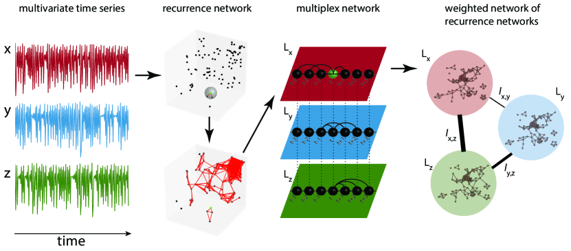
Figure 1: Illustration of the procedure for generating network structures from a multivariate time series:
multivariate time series $\rightarrow$ recurrence networks $\rightarrow$ multiplex recurrence network $\rightarrow$ weighted network of recurrence networks. Dashed lines between multiplex network’s layers connect all layers to all.

II.1 Recurrence Networks

A time series $\{u_{i}\}_{i=1}^{N}$ can be reconstructed as a trajectory (Eq. 1) in its phase space with time delay embedding (Packard et al., 1980)

$$\mathbf{x}_{i}=(u_{i},u_{i+\tau},...,u_{i+\tau(M-1)}),$$ (2)

where $M$ is the embedding dimension which can be found by a false nearest neighbours approach and $\tau$ is the embedding delay which can be computed by mutual information or auto-correlation (Kantz and Schreiber, 1997).

Two state vectors of the reconstructed time series are considered to be recurrent if the second vector falls into the neighbourhood (an $\epsilon$-radius sphere) of the first vector. For the trajectory $\vec{x}_{i}$ $(i=1,\ldots,N,\vec{x}_{i}\in\mathbb{R}^{M})$, the adjacency matrix of RN, $\mathbf{A}$, is defined as

$$A_{i,j}(\epsilon)=\Theta\bigl{(}\epsilon-\left\|\vec{x}_{i}-\vec{x}_{j}\right\|\bigr{)}-\delta_{i,j},\;i,j=1,\ldots,N,$$ (3)

where $N$ is the trajectory length, $\Theta(\cdot)$ is the Heaviside function, $\left\|\,\cdot\,\right\|$ is the Euclidian norm and $\delta_{i,j}$ is the Kronecker delta ($\delta_{i,j}=1$ if $i=j$, otherwise $\delta_{i,j}=0$) Marwan et al. (2009); Eroglu et al. (2014b).

A RN is constructed in the following way: Consider the time points of a time series as nodes of a network; if the nodes are sufficiently close to each other, in other words, if the space vectors are neighbours, then a link between them is drawn. $\mathbf{A}$ represents the network, where $A_{i,j}=1$ if $i$ and $j$ are connected, otherwise $A_{i,j}=0$.

In all recurrence based applications, the threshold $\epsilon$ is an arbitrarily selected small number. The selection of $\epsilon$ can affect the results easily. In order to have a reasonable analysis, some threshold selection techniques were proposed Ahlstrom et al. (2006); Marwan et al. (2007); Eroglu et al. (2014b). However none of them is a certain way to choose the threshold. To be consistent, in this work we always used the way which depends on the standard deviation of the time series Schinkel et al. (2008).

II.2 Multiplex and Weighted Recurrence Networks

Multiplex structure. In this work, an $m$-layer multiplex network is constructed by RNs. For $m$-dimensional multivariate time series, we can create $m$ different RNs which have the same number of nodes and each node is labeled by its associated time. These networks will form the different layers of a multilayer network. The layers are connected each other with the same time labeled nodes. This procedure requires that the time sampling is the same for all of the used time series. If a multilayer network consists of $m$-layers which has the same number of nodes and the connections between layers are only between a node and its counterpart in the other layers, then we call such networks “multiplex”. Networks, transformed from multivariate time series, are compatible with the definition of multiplex networks, because each node is uniquely assigned to a certain time point of the multivariate time series, i.e., we will find the equally time-labelled nodes in all layers.

We consider an $m$-dimensional multivariate time series $\{\bm{u}(t)\}_{t=1}^{N}$, with $\bm{u}(t)=(u_{1}(t),u_{2}(t),\ldots{},u_{m}(t))\in\mathbb{R}^{m}$ for any value of $t$. Then, the RN of the $\kappa$th component of $\bm{u}(t)$ is created and located into the associated layer $\kappa$ of the multiplex network. For an example with $N=3$ time series these steps are illustrated in Fig. 1. First, we have three time series and construct a phase space for each signal. The RN of the $\kappa$th component of the time series is calculated by Eqs. (2)–(3) and then placed in to layer $\kappa$. We denote the adjacency matrix of the $\kappa$th layer as $A^{[\kappa]}={a_{ij}^{[\kappa]}}$ and $a_{ij}^{\kappa}=1$ if nodes $i$ and $j$ are connected in layer $\kappa$, $a_{ij}^{\kappa}=0$ otherwise. The giant adjacency matrix describing the entire multiplex network is denoted by

$$\mathcal{A}=\left[\begin{array}[]{ccccc}\mathbf{A}^{[1]}&\bf{I}$$_{N}&\ldots&\bf{I}$$_{N}\\ \bf{I}$$_{N}&\mathbf{A}^{[2]}&\ddots&\vdots\\ \vdots&\ddots&\ddots&\bf{I}$$_{N}\\ \bf{I}$$_{N}&\ldots&\bf{I}$$_{N}&\mathbf{A}^{[m]}\end{array}\right]$$ (4)

where $\bf{I}$_N is the identity matrix of size $N$.

In order to measure the similarity between layer $\kappa$ and $\gamma$ of the MRN, we use the interlayer mutual information $I_{\kappa,\gamma}$ Lacasa et al. (2015):

$$I_{\kappa,\gamma}=\sum_{k^{[\kappa]}}\sum_{k^{[\gamma]}}P(k^{[\kappa]},k^{[\gamma]})\log\frac{P(k^{[\kappa]},k^{[\gamma]})}{P(k^{[\kappa]})P(k^{[\gamma]})}$$ (5)

where $P(k^{[\kappa]})$ and $P(k^{[\gamma]})$ are the degree distributions of RNs at layer $\kappa$ and $\gamma$ respectively, and $P(k^{[\kappa]},k^{[\gamma]})$ is the joint probability of the existence of nodes which has $k^{[\kappa]}$ degree at layer-$\kappa$ and $k^{[\gamma]}$ at layer-$\gamma$. The degree distribution $P(k)$ is a probability distribution function which holds a general structure information that how many nodes have each degree. The mutual information measures how much a system is similar to another. Instead of computing mutual information between original time series, degree distributions are considered in Eq. 5. The difference to the commonly used direct mutual information of time series is that $I_{\kappa,\gamma}$ does not compare the probability of states (estimated from the time series) but the topological structure in the phase space based on the recurrences (using the recurrence matrix). This similarity measure $I_{\kappa,\gamma}$ quantifies the information flow between the multiplex networks and, thus, the characteristical behaviour of the system. The average of the quantity of $I_{\kappa,\gamma}$ over all possible pairs of layers of MRN, gives a scalar variable $I=\left<I_{\kappa,\gamma}\right>_{\kappa,\gamma}$ which captures the mean similarity of the degree distributions of the RNs, i.e., the order of coherence in the system.

Another measure to quantify the coherence of the original multivariate system by the MRN is the average edge overlap:

$$\omega=\frac{\sum_{i}\sum_{j>i}\sum_{\kappa}a_{ij}^{[\kappa]}}{m\sum_{i}\sum_{j>i}\left(1-\delta_{0,\sum_{\kappa}a_{ij}^{[\kappa]}}\right)}$$ (6)

where $\delta_{ij}$ is the Kronecker delta symbol. This measure represents the average number of identical edges over all layers of the multiplex network Lacasa et al. (2015). Like the interlayer mutual information Eq. (5), $\omega$ estimates the similarity and coherence with averaged existence of overlapped links from node-$i$ to $j$ between all layers $\kappa$ and $\gamma$. Note that $\omega$ can take values in the interval $[1/m,1]$, if the link between $i$ and $j$ occurs in only different layers $\omega=1/m$, i.e., $a_{ij}^{[\kappa]}=1$ and $a_{ij}^{[\gamma]}=0,\,\forall\gamma\neq\kappa$. If all links are identical in all layers then $\omega=1$.

Weighted structure. Another approach is the projection of all layers onto one weighted network representation. Now we consider each single layer of an MRN as a node and weighted edges between nodes $\kappa$ and $\gamma$ are determined by the quantity $I_{\kappa,\gamma}$, Eq. (5).

In order to quantify high-dimensional systems, converting multilayer systems to weighted structures is computationally a very efficient approach. The adjacency matrix of the multiplex network $\mathcal{A}$ is a giant matrix ($Nm\times Nm$), but in the weighted network case the size of the matrix is only $N\times N$. Furthermore, the quantification of weighted networks is a well-developed analysis Barrat et al. (2004); Boccaletti et al. (2006). Among many measures of weighted networks, we use the clustering coefficient $\mathcal{C}_{w}$ and the average path length $\mathcal{L}_{w}$ in order to detect the transitions between different dynamical regimes. The weighted network clustering coefficient is given by

$$\mathcal{C}_{w}=\frac{1}{m}\sum_{\kappa}\frac{1}{k_{\kappa}(k_{\kappa}-1)}\sum_{\gamma}\sum_{\beta}(I_{\kappa,\gamma}I_{\kappa,\beta}I_{\gamma,\beta})^{\frac{1}{3}}$$ (7)

where $k_{\kappa}$ is the degree of node $\kappa$. The average shortest path length of the weighted network is

$$\mathcal{L}_{w}=\sum_{\kappa,\gamma\in V}\frac{d(\kappa,\gamma)}{m(m-1)},$$ (8)

where $V$ is the set of nodes (layers of multiplex network) in the weighted network and $d(\kappa,\gamma)$ is the weighted shortest path length between nodes $\kappa$ and $\gamma$.

Both MRN measures, $I$ and $\omega$, represent the similarities in the linking structures of the RNs and have higher values for more similar ones. For example, for periodic systems, even if there is phase difference, the corresponding RNs would be rather similar, resulting in high values for $I$ and $\omega$. When the systems are more chaotic and have finally a more different recurrence structure, $I$ and $\omega$ will decrease. This is similar for $\mathcal{C}_{w}$, since in periodic cases the number of triangle structures in networks is increasing. However, it is opposite for $\mathcal{L}_{w}$ because the diameter of a denser network is in general smaller.

III Coupled Map Lattices

As a first application, we consider multi-component dynamical systems, namely coupled map lattices (CMLs), which are discrete-time models of diffusively coupled oscillators on a ring model of $m$ sites. CMLs are well-studied dynamical systems that model the behavior of non-linear systems and exhibit a variety of phenomena Kaneko (1992).

$$x^{[\kappa]}_{t+1}=(1-\varepsilon)f(x^{[\kappa]}_{t})+\frac{\varepsilon}{2}\bigl{(}f(x^{[\kappa-1]}_{t})+f(x^{[\kappa+1]}_{t})\bigr{)},$$ (9)

CMLs have been analyzed with various techniques to quantify their very rich dynamics. Now we compare multiplex and regular RN approaches for CMLs of $m=5$ diffusely coupled chaotic logistic maps $f(x)=4x(1-x)$, which show interesting dynamics in the range of the control parameter $\varepsilon\in[0,0.4]$ studied here with an increment of $\Delta\varepsilon=0.005$. For instance, pattern selections, high-dimensional chaos regimes, many different forms of partially synchronized chaotic states occur. We compute a time series of length $N=15,000$ for each value of $\varepsilon$. In order to discard transients, we delete the first 10,000 values, resulting in time series consisting of 5,000 values that have been used for all analyses of the CMLs in this paper. All simulations of CMLs are repeated and averaged over 100 realizations, since the system strongly depends on the initial conditions. In order to compare MRN and RN techniques, we construct a five-dimensional phase space for regular RN and five separated single RN for each layer of MRN.

For consistency, we use a recurrence threshold that is proportional to the standard deviation $\sigma$ of the data Marwan et al. (2007). In this work, we use $\epsilon=0.05\sigma$. The logistic map is a one-dimensional dynamical system, therefore embedding is not required for applying recurrence networks in the layers of MRN.

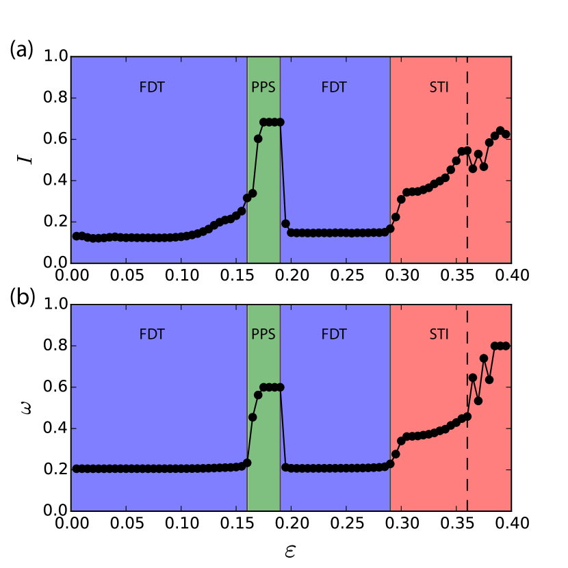
Figure 2: Results for $m=5$ CMLs (Eq. 9), (a) average mutual information ($I$), and (b) average edge overlap ($w$) of MRN.

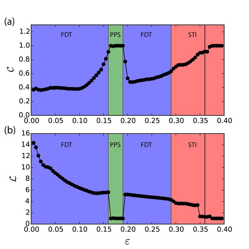
Figure 3: Results for $m=5$ diffusively coupled map lattices CMLs, (a) clustering coefficient $\mathcal{C}$, and (b) average path length $\mathcal{L}$ of the (regular) recurrence network.

Although both techniques could detect the transitions from fully developed turbulence (FDT), $\varepsilon\in[0.0,0.15]$ and $\varepsilon\in[0.19,0.285]$, to periodic pattern selection (PPS), $\varepsilon\in[0.15,0.19]$, the RN approach cannot distinguish the transition from FDT to spatio-temporal intermittency (STI), $\varepsilon\in[0.285,0.4]$ (Figs. 2, 3). Multiplex network’s measures ($I$ and $\omega$) can recognize every single transition and, especially $\omega$, can distinguish splitting of trajectories into two attractors in STI at $\varepsilon=0.36$ very clearly (Fig. 2). The MRNs are more sensitive to regime changes than the RNs as well as the MRNs are applicable on large system sizes when RNs are not suitable to deal with them.

Large systems. Simultaneous analysis of interacting components of a system is very important for deep understanding of the underlying dynamics. The RN approach is not an appropriate technique to analyze such systems, because while the number of degrees of freedom is increasing, the size (volume) of its phase space is getting larger as well. Therefore, in order to analyze such systems, we need very long data sets proportional to the size of the dimension of the system for establishing recurrences. Although the recurrence based analyses nicely deals with analyzing short time series, finding long data is a common problem in time series analysis. However, MRNs overcome this problem since they use each component of the system as a layer of the giant network.

In this application, we use the same parameters of the RN and the isolated dynamics as in the small system size one. Fig. 4 presents the results of the MRN for $m=200$ diffusely coupled logistic maps, which possess one more different regime than the small system, called Brownian motion of defect (BMD), $\varepsilon\in[0.12,0.14]$. FDT occurs for $\varepsilon\in[0.0,0.12]$ and $\varepsilon\in[0.19,0.30]$, STI is observed for $\varepsilon\in[0.14,0.16]$ and PPS for $\varepsilon\in[0.16,0.19]$. These regimes were observed and presented in detail in Kaneko (1989); Kaneko and Tsuda (2001). The MRN distinguishes the transitions between different regimes clearly and this analysis is the first recurrence based approach to detect these transitions in a large coupled system.

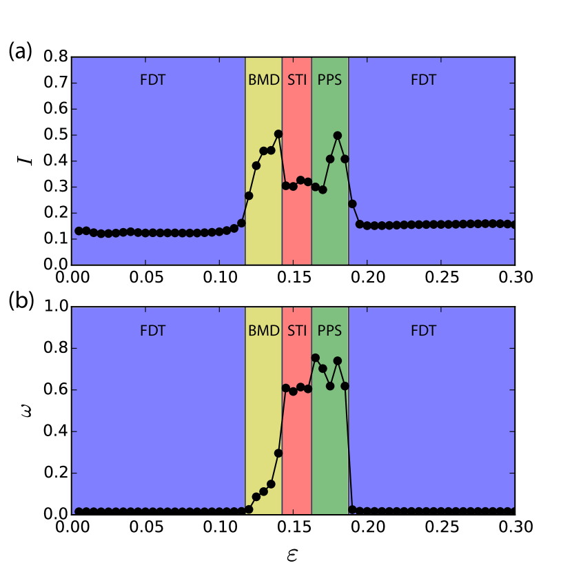
Figure 4: Results for $m=200$ diffusively coupled map lattices CMLs (a) average mutual information ($I$), (b) average edge overlap ($w$) of multiplex network.

Instead of analysing the giant adjacency matrix of MRN, we can investigate the same system with taking advantage of the well-developed weighted network analysis. Among the weighted network measures, the clustering coefficient Eq. (7) and the average shortest path length Eq. (8) are computed for the associated network and the results are given in Fig. 5. As the results of MRN, the related weighted network shows the transition very clearly. For large enough multi-dimensional systems, both approaches can be used.

The coupled maps are identical. In the fully developed chaotic regime they are not synchronized, i.e., the evolution of the (chaotic) maps due to their distinct initial conditions is different. Varying the coupling constant $\varepsilon$ changes the dynamical regime of the maps. According to the high chaos in the FDT, each RN has a rather different topology compared to the others, i.e., all the single layers of the MRN are quite different. The BMD is a less chaotic regime, thus, the single layers of the MRN are less different than in the FDT regime (increasing the inter-layer similarity). The PPS and STI regimes are closer to each other as both regimes exhibit periodic dynamics but at different scales. Therefore, distinguishing the transition between PPS and STI is the hardest task. Nevertheless, $I$ and $\omega$ are able to detect the corresponding regime transitions. However, $\omega$ performs better, because it is a spatio-temporal measure, i.e., it checks the existence of edges at the same locations in the different layers where the calculation for $I$ does not take the nodes’ identities into account.

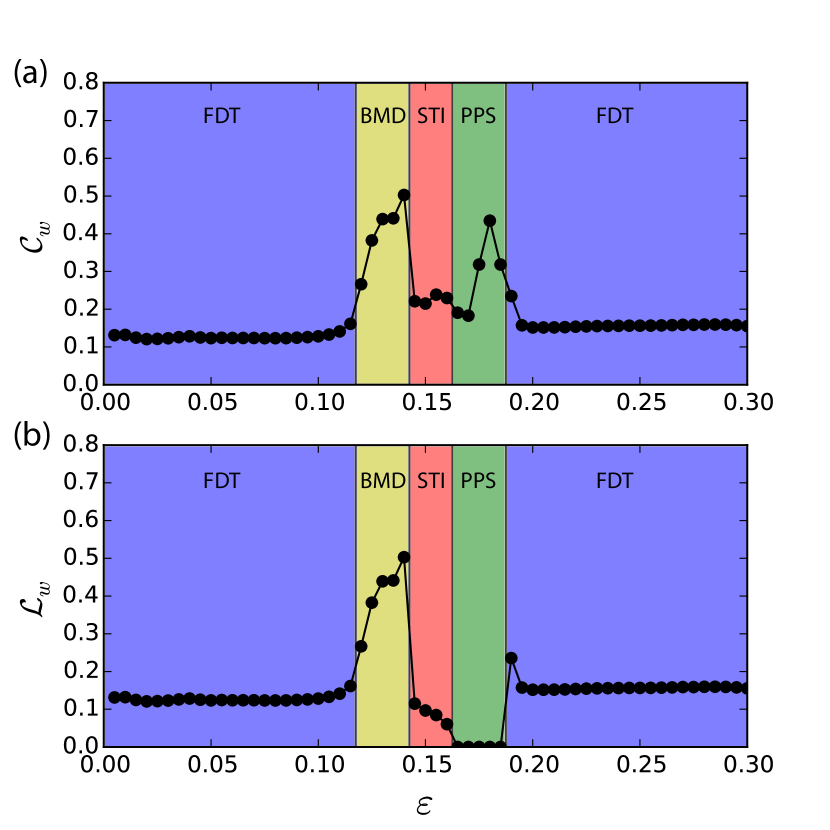
Figure 5: Results for $m=200$ diffusively coupled map lattices CMLs (a) clustering coefficient of weighted network $\mathcal{C}_{w}$, (b) average path length of weighted network $\mathcal{L}_{w}$

IV Real-world example – multivariate palaeoclimate analysis

So far we have been testing the performance of the new MRN method using prototypical models. As a real-world application with changing dynamics and with several variables, we treat a palaeoclimate problem. The investigation of the linkage between the climate conditions and specific environmental responses, as well as of changes in these relationships represent an important scientific challenge in palaeoclimatology and ecology in order to improve the understanding of climate impacts and feedback mechanisms. Information on past vegetation is useful to understand the palaeoecological processes linking climate and biosphere changes. Vegetation dynamics depends strongly on the environmental conditions and changes in the vegetation dynamics can, therefore, indicate critical changes in the environment (anthropogenic or climate impact).

Pollen assemblages collected from lake sediments are commonly used proxies for palaeoecological and palaeoclimate investigations. Here we focus on the precisely dated Late Pleistocene-Holocene pollen record (last 16,500 years (16.5 kyr BP)) from the Sihailongwan Lake (42^∘170^′ N, 126^∘360^′ E), located in the Longgang volcanic field, Jilin Province, NE China (Fig. 6) Stebich et al. (2009, 2015a, 2015b).

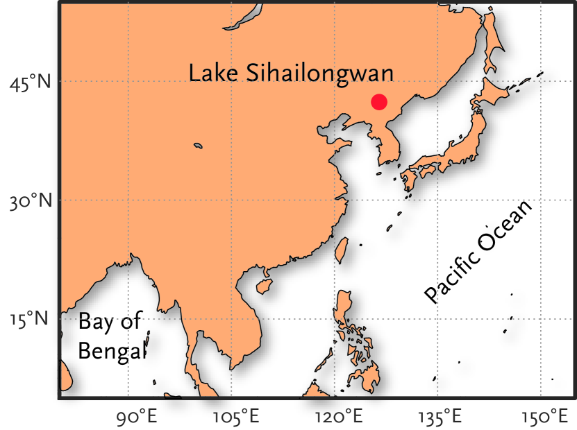
Figure 6: Location of the Lake Sihailongwan from where the pollen record for this study was sampled.

The Sihailongwan Lake is situated near the northern edge of the Asian summer monsoon system. Originally the Sihailongwan pollen record consists of 103 different pollen taxa, whereby several of them contain redundant information. We, therefore, selected seven tree pollen taxa (Pinus koraiensis, Betula, Carpinus, Juglans, Quercus, Ulmus, Fraxinus and one herbaceous genus (Artemisia), representing typical regional vegetation elements with different sensitivities on specific environmental conditions during the past 16.5 kyr BP (Fig. 7).

Since, the pollen record is irregularly sampled, we first interpolate the data into $N=3,500$ points leading to the time resolution $\Delta t=t_{i+1}-t_{i}\approx 4.95$ years $\forall\,i\in[0,N-1]$. In order to analyze the temporal variation in the environmental dynamics, we apply a sliding window approach consisting of 150 data points per window. By this choice, each window covers about $740$ years and is suitable to represent regime changes in the environmental dynamics. MRN is created for each window one by one as the window slides over the time series with 90% overlap.

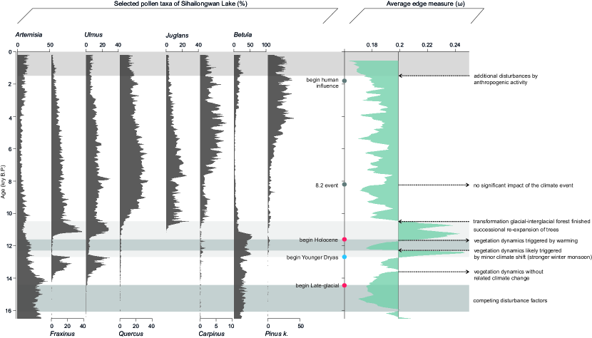
Figure 7: Pollen data set from Sihalongwan Lake (left) and derived average edge measure $\omega$ calculated in moving windows (right). The basevalue of the shading (0.199) marks the upper 95% confidence interval, i.e., exceeding this value corresponds with highly significant increase of $\omega$. The grey shaded bands mark important environmental and climate transitions (see text).

The application of the MRN technique to the multivariate pollen data set reveals distinct fluctuations of $\omega$ (Fig. 7). A bootstrapping statistical test is applied to evaluate these variations with respect to the null-hypothesis that multivariate dynamics is constant over time within 95% confidence Marwan et al. (2013).

The considered measure $\omega$ quantifies the amount of similar dynamics in the different pollen taxa. The higher $\omega$, the more similar vary the different vegetation types in the sense of recurrence properties. This means, it is not necessary that the pollen abundances go into the same directions, but that, e.g., periodical variations are similar. Low $\omega$ values indicate, in contrast, less similar behavior. This could happen, e.g., when the system is disturbed and some vegetation populations recover faster than others.

The pollen assemblages reveal relatively open, cold-dry adapted vegetation at Sihailongwan at the end of the pleniglacial. Starting at 16.0 kyr BP, we find a decrease of $\omega$ until 15.0 kyr BP. The apparent decrease of the similarity in the floristic response likely results from rather instable environmental conditions or competing factors influencing the vegetation dynamics. The instable environment at Sihailongwan is strongly evidenced by the sediment composition during this time interval. In particular, the occurrence of graded event layers with reworked soil material implies prevailing permafrost conditions with reduced seepage and erosion events during the final stage of the last glacial period Stebich et al. (2009). Moreover, the youngest Heinrich event (H1; 16.0 and 14.6 kyr BP), may have resulted in stronger winter monsoon Wang (2001). By contrast, the ongoing change of CO₂ from the glacial to the interglacial level might have individually affected both the physiology of the prevailing plants, and the vegetation dynamics in an increasingly less moisture-stressed environment Cowling and Sykes (1999); Monnin et al. (2004).

Subsequent to the H1 event, the environmental conditions during the Late-glacial interstadial changed to warmer and moister climate, obviously related with a general change in the regional vegetation to one of more similar vegetation dynamics. The short positive excursion of $\omega$ at 13.6 kyr BP is, however, clearly not related to a climate shift, but most likely results from a change in interspecific competition after reaching a critical population density of Fraxinus Stebich et al. (2009).

The Younger Dryas temperature decline about 12.7 kyr BP ago is one of the most prominent climate changes observed in Northern Hemisphere palaeoclimate records. Noticeable changes in the Sihailongwan pollen record provide a clear indication of a Younger-Dryas-like cooling in NE China beginning at 12.7 kyr BP. Unlike the abrupt termination of the Younger Dryas in the North Atlantic evidence, the more gradual changes of pollen assemblages indicate a successive substitution of the prevailing boreal woodland by species-rich broadleaf deciduous forests at the Sihailongwan lake during the first millennium of the Holocene (11.7 and 10.7 kyr BP).

Our MRN analysis reveals significant high values of $\omega$ in the period between 12.7 and 10.5 kyr BP, which are interrupted by an abrupt drop in $\omega$ between about 12.3 and 11.7 kyr BP. The timing of this prominent change in vegetation dynamics corresponds to the recently detected bipartition of the Younger Dryas at Suigetsu Lake (Japan) Schlolaut et al. (2017), but neither the composition of pollen assemblages nor the sediments of the Sihailongwan sequence reveal a substantial environmental shift at 12.3 kyr BP. It is likely, that the ecosystem at Sihailongwan Lake may not be as sensitive to changes in winter conditions as the Japanese site Schlolaut et al. (2017), so that the climate shift may have influenced the intrinsic vegetation dynamics at Sihailongwan, but could not trigger substantial floristic and/or landcover changes.

At approximately 10.7 kyr BP, the dynamic spread of thermophilous Juglans and a more gradual increase of Quercus mark a shift in the vegetation composition to oak- and walnut-rich mixed conifer hardwood forests. Subsequent to this transition, the MRN analysis data indicate persistent vegetation dynamics, but the general shift to lower $\omega$ values implies less similar behaviour of the pollen taxa. Interestingly, a shift in $\omega$ can be observed around 8.2 kyr BP, which might be related to the most prominent drop of the global temperatures during the Holocene. However, as its amplitude does not exceed that of other Holocene changes in vegetation dynamics, the shift does no€™t prove a significant impact of the 8.2 event on the vegetation in NE China.

While substantial human impact cannot be traced by the pollen assemblages, monsoon changes, forest succession dynamics and flowering activity may therefore primarily drive the observed dynamics in the pollen values/vegetation at Sihailongwan throughout the Holocene. Nevertheless, weak indication of farming activity in conjunction with fires and modest grazing may explain the minor shift to lower ω values from 1.8 yrs BP.

Taken together, in our example we find that the patterns of vegetation dynamics are related to both intrinsic vegetation dynamics and external disturbance factors like climate changes, erosion or human impact. Obviously, the different vegetation types behave more similar when one environmental factor acts as the dominant driving force. This is particularly evident at the change to cooler and drier conditions at the beginning of Younger Dryas. Also the rapid mass expansion or the collapse of one or more tree species can have a similar effect on the dynamics of vegetation, as detected in our example at 13.6 kyrs BP and throughout the first millennium of the Holocene. On the other hand, less similar behaviour of the vegetation results from weaker or competing disturbance factors. Our example demonstrates that the new developed MRN technique goes beyond the classical interpretation of the pollen amplitude variation as a proxy of environmental conditions. A better understanding of this part of the climate-biosphere interaction is of crucial importance as non-linear feedback mechanisms and tipping points cause high uncertainty and an unpredictable future for humankind Lenton et al. (2008); Rockstrom et al. (2009).

V Conclusions

In this study we have introduced a novel multiplex recurrence network (MRN) approach which allows us to analyze $m$-dimensional multivariate data simultaneously via joining $m$ recurrence networks (RNs) together. Analyzing and understanding the characteristics of single or low dimensional data with RNs is a known approach Donges et al. (2011); Donner et al. (2011b). Nevertheless, RN analysis of high dimensional systems is not trivial, because the increasing dimension of the phase space would require longer time series. However, studies of real-world problems are often linked with short time series and long time series are often not available. Our new approach considers each observation variable in its own phase space and combines them later on. Therefore, it is possible to analyze relatively short multivariate time series with MRNs.

Our extensive tests of the method have demonstrated that the MRN approach enables us to detect abrupt regime transitions accurately in large dimensional systems. It can be used to understand the underlying dynamical properties of prototypical models and real-world applications.

By analysing a pollen data set for the last 16 kyr, we are able to identify periods when different vegetation types behave more similar and periods of less similar behaviour. The changes in the vegetation dynamics coincide well with known climate transitions and the increasing human impact. This analysis goes beyond the classical interpretation of the pollen amplitude variation as a proxy of environmental conditions. This new view can provide insights into plant communities and their dynamics with respect to climate responses.

Especially for some research fields such as palaeoclimate (pollen taxa, planktonic samples etc), neuroscience (short time crises in EEG), economics (stock markets, currencies), where many dependent signals are collected at the same time, our method provides a quantitative and objective way to investigate their dynamics and detects hidden regime changes.

Acknowlegments

This work has been supported by German-Israeli Foundation for Scientific Research and Development (GIF), GIF Grant No. I-1298-415.13/2015 and the European Union’s Horizon 2020 Research and Innovation programme under the Marie Skłodowska-Curie grant agreement No. 691037 (QUEST).

References

- Poincaré (1890) H. Poincaré, Acta Mathematica 13, 1 (1890).
- Katok and Hasselblatt (1995) A. Katok and B. Hasselblatt, Introduction to the Modern Theory of Dynamical Systems (Cambridge University Press, Cambridge, 1995).
- Eckmann et al. (1987) J.-P. Eckmann, S. Oliffson Kamphorst, and D. Ruelle, Europhysics Letters 4, 973 (1987).
- Marwan et al. (2007) N. Marwan, M. C. Romano, M. Thiel, and J. Kurths, Physics Reports 438, 237 (2007).
- Trulla et al. (1996) L. L. Trulla, A. Giuliani, J. P. Zbilut, and C. L. Webber Jr., Physics Letters A 223, 255 (1996).
- Marwan et al. (2002) N. Marwan, N. Wessel, U. Meyerfeldt, A. Schirdewan, and J. Kurths, Physical Review E - Statistical, Nonlinear, and Soft Matter Physics 66, 1 (2002).
- Donges et al. (2011) J. Donges, R. Donner, M. Trauth, N. Marwan, H. Schellnhuber, and J. Kurths, Proceedings of the National Academy of Sciences 108, 20422 (2011).
- Jansen (1991) B. H. Jansen, International Journal of Bio-Medical Computing 27, 95 (1991).
- Kaplan et al. (1991) D. Kaplan, M. Furman, S. Pincus, S. Ryan, L. Lipsitz, and A. Goldberger, Biophysical Journal 59, 945 (1991).
- Riley et al. (1999) M. A. Riley, R. Balasubramaniam, and M. T. Turvey, Gait & Posture 9, 65 (1999).
- Neuman et al. (2009) Y. Neuman, N. Marwan, and D. Livshitz, Complexity 15, 28 (2009).
- Carrubba et al. (2012) S. Carrubba, A. Minagar, A. L. Chesson Jr., C. Frilot II, and A. A.Marino, Neurological Research 34, 286 (2012).
- Richards (1994) G. R. Richards, Quaternary Science Reviews 13, 709 (1994).
- Marwan et al. (2003) N. Marwan, M. H. Trauth, M. Vuille, and J. Kurths, Climate Dynamics 21, 317 (2003).
- Matcharashvili et al. (2008) T. Matcharashvili, T. Chelidze, and J. Peinke, Nonlinear Dynamics 51, 399 (2008).
- Ozken et al. (2015) I. Ozken, D. Eroglu, T. Stemler, N. Marwan, G. B. Bagci, and J. Kurths, Physical Review E 91, 062911 (2015).
- Eroglu et al. (2016) D. Eroglu, F. H. McRobie, I. Ozken, T. Stemler, K.-H. Wyrwoll, S. F. M. Breitenbach, N. Marwan, and J. Kurths, Nature communications 7, 1 (2016).
- Asghari et al. (2004) N. Asghari, C. Broeg, L. Carone, R. Casas-Miranda, J. C. C. Palacio, I. Csillik, R. Dvorak, F. Freistetter, G. Hadjivantsides, H. Hussmann, A. Khramova, M. Khristoforova, I. Khromova, I. Kitiashivilli, S. Kozlowski, T. Laakso, T. Laczkowski, D. Lytvinenko, O. Miloni, R. Morishima, A. Moro-Martin, V. Paksyutov, A. Pal, V. Patidar, B. Pecnik, O. Peles, J. Pyo, T. Quinn, A. Rodriguez, M. C. Romano, E. Saikia, J. Stadel, M. Thiel, N. Todorovic, D. Veras, E. V. Neto, J. Vilagi, W. von Bloh, R. Zechner, and E. Zhuchkova, Astronomy & Astrophysics 426, 353 (2004).
- Zolotova et al. (2009) N. V. Zolotova, D. I. Ponyavin, N. Marwan, and J. Kurths, Astronomy & Astrophysics 505, 197 (2009).
- Eroglu et al. (2014a) D. Eroglu, T. K. D. M. Peron, N. Marwan, F. A. Rodrigues, L. F. Costa, M. Sebek, and Z. Kiss, Physical Review E 042919, 1 (2014a).
- Marwan (2008) N. Marwan, European Physical Journal – Special Topics 164, 3 (2008).
- Grassberger and Procaccia (1983a) P. Grassberger and I. Procaccia, Physica D 9, 189 (1983a).
- Grassberger and Procaccia (1984) P. Grassberger and I. Procaccia, Physica D 13, 34 (1984).
- Zhang and Small (2006) J. Zhang and M. Small, Physical Review Letters 96, 3 (2006).
- Small (2013) M. Small, 2013 IEEE International Symposium on Circuits and Systems (ISCAS2013) , 2509 (2013).
- Lacasa et al. (2008) L. Lacasa, B. Luque, F. Ballesteros, J. Luque, and J. C. Nuño, Proceedings of the National Academy of Sciences of the United States of America 105, 4972 (2008), arXiv:0810.0920 .
- Lacasa et al. (2009) L. Lacasa, B. Luque, J. Luque, and J. C. Nuño, EPL (Europhysics Letters) 86, 30001 (2009).
- Lacasa et al. (2015) L. Lacasa, V. Nicosia, and V. Latora, Scientific Reports 5, 15508 (2015).
- Zhang et al. (2008) J. Zhang, J. Sun, X. Luo, K. Zhang, T. Nakamura, and M. Small, Physica D 237, 2856 (2008).
- Xu et al. (2008) X. Xu, J. Zhang, and M. Small, Proceedings of the National Academy of Sciences 105, 19601 (2008).
- Marwan et al. (2009) N. Marwan, J. F. Donges, Y. Zou, R. V. Donner, and J. Kurths, Physics Letters A 373, 4246 (2009).
- Donner et al. (2011a) R. V. Donner, M. Small, J. F. Donges, N. Marwan, Y. Zou, R. Xiang, and J. Kurths, International Journal of Bifurcation and Chaos 21, 1019 (2011a).
- Grassberger and Procaccia (1983b) P. Grassberger and I. Procaccia, Physical Review Letters 50, 346 (1983b).
- Afraimovich (1997) V. Afraimovich, Chaos 7, 12 (1997).
- Saussol et al. (2002) B. Saussol, S. Troubetzkoy, and S. Vaienti, Journal of Statistical Physics 106, 623 (2002).
- Saussol and Wu (2003) B. Saussol and J. Wu, Nonlinearity 16, 1991 (2003).
- Donner et al. (2011b) R. V. Donner, J. Heitzig, J. F. Donges, Y. Zou, N. Marwan, and J. Kurths, European Physical Journal B 84, 653 (2011b).
- Afsar et al. (2015) O. Afsar, D. Eroglu, N. Marwan, and J. Kurths, EPL (Europhysics Letters) 112, 10005 (2015).
- Ramírez Ávila et al. (2013) G. M. Ramírez Ávila, A. Gapelyuk, N. Marwan, T. Walther, H. Stepan, J. Kurths, and N. Wessel, Philosophical Transactions of the Royal Society A 371, 20110623 (2013).
- Feldhoff et al. (2012) J. H. Feldhoff, R. V. Donner, J. F. Donges, N. Marwan, and J. Kurths, Physics Letters, Section A: General, Atomic and Solid State Physics 376, 3504 (2012), arXiv:1301.0934 .
- Bianconi (2013) G. Bianconi, Physical Review E 87, 062806 (2013).
- Nicosia et al. (2013) V. Nicosia, G. Bianconi, V. Latora, and M. Barthelemy, Physical Review Letters 111, 058701 (2013), arXiv:1302.7126 .
- De Domenico et al. (2013) M. De Domenico, A. Solé-Ribalta, E. Cozzo, M. Kivelä, Y. Moreno, M. A. Porter, S. Gómez, and A. Arenas, Physical Review X 3, 041022 (2013).
- Kivelä et al. (2014) M. Kivelä, A. Arenas, M. Barthelemy, J. P. Gleeson, Y. Moreno, and M. a. Porter, Journal of Complex Networks 2, 203 (2014), arXiv:1309.7233 .
- Nicosia and Latora (2015) V. Nicosia and V. Latora, Physical Review E 92, 032805 (2015).
- Packard et al. (1980) N. H. Packard, J. P. Crutchfield, J. D. Farmer, and R. S. Shaw, Physical Review Letters 45, 712 (1980).
- Kantz and Schreiber (1997) H. Kantz and T. Schreiber, Nonlinear Time Series Analysis (University Press, Cambridge, 1997).
- Eroglu et al. (2014b) D. Eroglu, N. Marwan, S. Prasad, and J. Kurths, Nonlinear Processes in Geophysics 21, 1085 (2014b).
- Ahlstrom et al. (2006) C. Ahlstrom, P. Hult, and P. Ask (2006) pp. III688–III691.
- Schinkel et al. (2008) S. Schinkel, O. Dimigen, and N. Marwan, European Physical Journal: Special Topics 164, 45 (2008).
- Barrat et al. (2004) A. Barrat, M. Barthélemy, R. Pastor-Satorras, and A. Vespignani, Proceedings of the National Academy of Sciences of the United States of America 101, 3747 (2004), arXiv:0311416 [cond-mat] .
- Boccaletti et al. (2006) S. Boccaletti, V. Latora, Y. Moreno, M. Chavez, and D. U. Hwang, Physics Reports 424, 175 (2006).
- Kaneko (1992) K. Kaneko, Chaos 2, 279 (1992).
- Kaneko (1989) K. Kaneko, Physica D: Nonlinear Phenomena 34 (1989), 10.1016/S0378-4371(00)00431-3.
- Kaneko and Tsuda (2001) K. Kaneko and I. Tsuda, Complex Systems: Chaos and Beyond (Springer-Verlag Berlin Heidelberg, 2001).
- Stebich et al. (2009) M. Stebich, J. Mingram, J. Han, and J. Liu, Global and Planetary Change 65, 56 (2009).
- Stebich et al. (2015a) M. Stebich, K. Rehfeld, F. Schlütz, P. E. Tarasov, J. Liu, and J. Mingram, Quaternary Science Reviews 124, 275 (2015a).
- Stebich et al. (2015b) M. Stebich, K. Rehfeld, F. Schlütz, P. E. Tarasov, J. Liu, and J. Mingram, PANGAEA (2015b), 10.1594/PANGAEA.852704.
- Marwan et al. (2013) N. Marwan, S. Schinkel, and J. Kurths, Europhysics Letters 101, 20007 (2013).
- Wang (2001) Y. J. Wang, Science 294, 2345 (2001).
- Cowling and Sykes (1999) S. A. Cowling and M. T. Sykes, Quaternary Research 52, 237 (1999).
- Monnin et al. (2004) E. Monnin, E. J. Steig, U. Siegenthaler, K. Kawamura, J. Schwander, B. Stauffer, T. F. Stocker, D. L. Morse, J.-M. Barnola, B. Bellier, D. Raynaud, and H. Fischer, Earth and Planetary Science Letters 224, 45 (2004).
- Schlolaut et al. (2017) G. Schlolaut, A. Brauer, T. Nakagawa, H. F. Lamb, J. J. Tyler, R. A. Staff, M. H. Marshall, C. Bronk Ramsey, C. L. Bryant, and P. E. Tarasov, Scientific Reports 7, 44983 (2017).
- Lenton et al. (2008) T. M. Lenton, H. Held, E. Kriegler, J. W. Hall, W. Lucht, S. Rahmstorf, and H. J. Schellnhuber, Proceedings of the National Academy of Sciences of the United States of America 105, 1786 (2008).
- Rockstrom et al. (2009) J. Rockstrom, W. Steffen, K. Noone, A. Persson, F. S. Chapin III, E. F. Lambin, T. M. Lenton, M. Scheffer, C. Folke, H. J. Schellnhuber, B. Nykvist, C. A. de Wit, T. Hughes, S. van der Leeuw, H. Rodhe, S. Sorlin, P. K. Snyder, R. Costanza, U. Svedin, M. Falkenmark, L. Karlberg, R. W. Corell, V. J. Fabry, J. Hansen, B. Walker, D. Liverman, K. Richardson, P. Crutzen, and J. A. Foley, Nature 461, 472 (2009).