Deep Learning-based CSI Feedback and Cooperative Recovery in Massive MIMO

Abstract

In this paper, the correlation between nearby user equipment (UE) is exploited, and a deep learning-based channel state information (CSI) feedback and cooperative recovery framework, CoCsiNet, is developed to reduce feedback overhead. The CSI information can be divided into two parts: shared by nearby UE and owned by individual UE. The key idea of exploiting the correlation is to reduce the overhead used to feedback the shared information repeatedly. Unlike in the general autoencoder framework, an extra decoder and a combination network are added at the base station to recover the shared information from the feedback CSI of two nearby UEs and combine the shared and individual information, respectively, but no modification is performed at the UEs. For a UE with multiple antennas, a baseline neural network architecture with long short-term memory modules is introduced to extract the correlation of nearby antennas. Given that the CSI phase is not sparse, two magnitude-dependent phase feedback strategies that introduce statistical and instant CSI magnitude information to the phase feedback process are proposed. Simulation results on two different channel datasets show the effectiveness of the proposed CoCsiNet.

1 Introduction

Massive multiple-input multiple-output (MIMO) is regarded as a critical technology in future wireless communications [1, 2, 3]. Spectral efficiency can be dramatically improved in massive MIMO systems, which use numerous antennas at the base station (BS)[4]. The performance gain achieved by this technology primarily comes from spatial multiplexing in addition to diversity, which relies on the knowledge of the instantaneous uplink and downlink channel state information (CSI) at the BS. Therefore, the quality of available CSI at the BS directly affects the performance of massive MIMO systems.

The uplink CSI can be estimated at the BS by the pilots sent from the user equipment (UE). In time-division duplexing systems, the downlink CSI can be inferred from the uplink CSI by using channel reciprocity. In frequency-division duplexing (FDD) systems, which are widely employed by cellular systems, slight reciprocity exists between the uplink and downlink channels. Consequently, inferring the downlink CSI using only the uplink CSI is impossible. To obtain the downlink CSI, the BS should first transmit pilot symbols for the UE to estimate CSI locally [5]. Then, the UE feeds the estimated CSI back to the BS. The feedback overhead linearly scales with the product of the numbers of antennas at the BS and the UE, and is extremely large in massive MIMO systems, which occupy precious bandwidth source and are sometimes unaffordable [6]. Therefore, a technique must be developed to reduce feedback overhead efficiently while exerting negligible negative effects on system performance in FDD systems.

One well-known promising technique is compressive sensing (CS) theory via exploiting the CSI sparsity in certain domains [7]. In [8], the sparsity in the spatial-frequency domain due to the short distance between antennas is exploited to compress CSI and reduce feedback overhead. In [9], a distributed compressive downlink channel estimation and feedback scheme uses the hidden joint sparsity structure of CSI resulting from shared local scatterers. Although existing CS-based methods can greatly reduce feedback overhead [10], two main problems remain. The reconstruction based on the compressed CSI at the BS can be regarded as an optimization problem that is solved by iterative algorithms, which demand substantial time and computing sources. During the reconstruction phase, extra expert knowledge, such as the correlation of CSI to the nearby UE, is usually ignored.

Since the success achieved in the ImageNet competition, deep learning (DL) has made tremendous progress in computer vision and natural language processing [11]. The communication community has recently shown great interest in applying DL to improve the performance of communication systems [12, 13, 14]. A totally data-driven end-to-end communication system based on the autoencoder architecture is proposed in [15, 16] where DL-based encoder and decoder play the role of transmitter and receiver, respectively. DL is also widely used to enhance certain blocks of conventional communication systems, such as channel estimation [17, 18] and joint channel estimation and signal detection [19, 20].

DL is first applied to the CSI feedback in [21] based on the autoencoder architecture, where the encoder at the UE and the decoder at the BS perform compression and reconstruction, respectively. The compression of the hidden layers forces the encoder to capture the most dominant features of the input data, that is, compressing the CSI. Given its numerous potentials, such as feedback accuracy and reconstruction speed, DL-based CSI feedback has become an active research area in communications, and related works can be divided into four main categories[22]:

• Exploiting expert knowledge and extra correlation in massive MIMO systems. The long short-term memory (LSTM) architecture adopted in [23] extracts the temporal correlation of time-varying channels. In [24], CSI magnitude and phase are compressed, and uplink CSI magnitude is used to help recover downlink CSI magnitude during the reconstruction phase at the BS.

• Designing novel neural network (NN) architectures. This kind of work focuses on improving feedback performance by introducing novel NN architectures in computer vision to the CSI feedback problem, including joint convolutional residual network [25] and multi-resolution convolutional architecture [26]. In [27], the convolutional kernel size is changed from $3\times 3$ to $7\times 7$ to enlarge the receptive field, thereby exhibiting the CSI sparsity characteristic well.

• Quantization and entropy encoding. Given that the UE must feed the bitstream back rather than the float-point number in practical digital systems, the encoder module should be followed by a quantization module. After comparing the performance of uniform and non-uniform quantization in DL-based CSI feedback, an offset NN is introduced to minimize the quantization distortion in [27]. Given that the quantization operation is non-differentiable, its gradient is set as one in [25]. Moreover, to reduce feedback overhead further, an entropy coding module following a quantization module is used to reduce the feedback bits further in [28]. Unlike other quantization strategies, a binary representation is exploited in [29] to generate bitstreams.

• Tackling the deployment problem. Some new problems appear when deploying the DL-based CSI feedback method. A multiple-rate CSI feedback framework is proposed in [27] to address different compression ratios by using a single network. Fully connected (FC) layers are replaced by fully convolutional layers in [28], enabling the same NNs to work with different CSI dimensions. Feedback error and delay are considered in [30]. In [31], network pruning and the quantization technique are applied to CSI feedback, greatly reducing the storage and computational requirement of NNs. In addition,the security of DL-based analog CSI feedback under adversarial attack is analyzed in [32].

Many studies [33, 34, 35, 36, 37, 38] observe that the CSI of nearby users may share deterministic multipath components and have similar sparsity structures due to some shared local scattering clusters, which have been widely exploited in CS-based channel estimation. From [38], the correlation of all nearby UEs in a circle with a radius of 2m is over 0.48 when the BS is equipped with 64 antennas. The above observation can become increasingly common as the device density grows to hundred(s) per cubic meter in the future [2]. Therefore, the correlation of nearby UE should be exploited to reduce feedback overhead and improve feedback performance further.

In this paper, a cooperative CSI feedback NN, called CoCsiNet, is developed. Specifically, CSI magnitude and phase are separately fed back in the proposed CoCsiNet, rather than together as complex channel gains. In the CSI magnitude feedback phase, the CSI magnitude information is divided into two parts: shared by nearby UEs and owned by individual UEs. The key idea of exploiting the correlation is to reduce the overhead used to feed back the shared information repeatedly. These two kinds of information are automatedly learned from the data and combined at the BS by using an end-to-end approach. By contrast, CSI phase is not sparse and is difficult to compress greatly. A highly accurate phase feedback is unnecessary for CSI with a small magnitude. Inspired by [24], two magnitude-dependent phase feedback (MDPF) NNs are proposed by introducing the statistical and instant magnitude information to the NN for the phase feedback. Our contributions in this paper are summarized as follows:

• Cooperation mechanism is introduced to DL-based CSI feedback. CSI magnitude information is divided into two parts as in [36]: shared by nearby UE and owned by individual UE. An extra shared decoder is introduced to recover the shared information from the feedback bits of two nearby UE.

• An autoencoder-based feedback framework is developed. For UE with multiple antennas, the LSTM architecture is added to the decoder at the BS to exploit the correlation of CSI to different antennas at the same UE.

• To generate the bitstreams at the UE, two representative methods (i.e., quantization and binarization) are investigate and adopted to the DL-based CSI feedback.

• To compress the CSI phase, which is not sparse and is usually difficult to compress, two MDPF frameworks are proposed, where the statistical and instant magnitude information are introduced to the NNs.

Given that this paper aims to improve CSI feedback accuracy by introducing extra correlation among nearby UEs, only some simple NN architectures are adopted. More performance gains can be achieved if more advanced NN architectures are introduced, but it is out of this paper’s scope.

The rest of this paper is organized as follows. Section 2 introduces the massive MIMO channel model and the CSI feedback process. Section 3 presents the cooperative CSI feedback strategy and the NN framework and then describes the baseline NN architecture, the bitstream generation, and the CSI phase feedback strategy. Section 4 provides the numerical results of the proposed methods and demonstrates the mechanism of CoCsiNet via parameter visualization. Section 5 finally concludes our paper.

2 System Model

After introducing the massive MIMO channel model in this section, the DL-based CSI feedback process is described.

2.1 Massive MIMO Channel Model

Considering a massive MIMO system, the BS and the UE are equipped with $N_{t}$ ($\gg 1$) antennas and $N_{r}$ ($\geq 1$) antennas, respectively. According to the spatial multipath channel model [39], the downlink channel matrix, $\tilde{\textbf{H}}\in\mathbb{C}^{N_{r}\times N_{t}}$, can be written as

$$\tilde{\textbf{H}}=\sqrt{\frac{N_{r}N_{t}}{N_{c}}}\sum_{l=1}^{N_{c}}g_{l}\textbf{a}_{r}(\varphi_{r,l})\textbf{a}_{t}^{H}(\varphi_{t,l}),$$ (1)

where $N_{c}$ is the total path number; $g_{l}\sim\mathcal{CN}(0,1)$ denotes the complex gain of the $l$-th path; $\textbf{a}_{r}(\cdot)$ and $\textbf{a}_{t}(\cdot)$ are the steering vectors of the receiver and transmitter; $\varphi_{r,l}$ and $\varphi_{t,l}$ represent the angle-of-arrival (AoA) and the angle-of-departure (AoD), respectively. If the BS and the UE are all equipped with uniform linear array (ULA) antennas, then their steering vectors can be written as

$$\textbf{a}_{r}(\varphi_{r,l})=\sqrt{\frac{1}{N_{r}}}[1,e^{\frac{-j2\pi d\sin(\varphi_{r,l})}{\lambda}},\quad\cdot\cdot\cdot\quad,e^{\frac{-j2\pi d(N_{r}-1)\sin(\varphi_{r,l})}{\lambda}}]^{T},$$ (2)

$$\textbf{a}_{t}(\varphi_{t,l})=\sqrt{\frac{1}{N_{t}}}[1,e^{\frac{-j2\pi d\sin(\varphi_{t,l})}{\lambda}},\quad\cdot\cdot\cdot\quad,e^{\frac{-j2\pi d(N_{t}-1)\sin(\varphi_{t,l})}{\lambda}}]^{T},$$ (3)

where $\lambda$ and $d$ denote the carrier wavelength and the antenna element spacing, respectively. The BS is usually located at a high building, and channel path number $N_{c}$ is limited due to the few scatterers. Therefore, the CSI matrix H in the angle domain is sparse [40], which can be obtained through discrete Fourier transform (DFT) as

$$\mathbf{H}=\mathbf{F}_{\rm r}\tilde{\textbf{H}}\mathbf{F}_{\rm t},$$ (4)

where $\mathbf{F}_{\rm r}$ and $\mathbf{F}_{\rm t}$ are $N_{\rm r}\times N_{\rm r}$ and $N_{\rm t}\times N_{\rm t}$ DFT matrices, respectively.

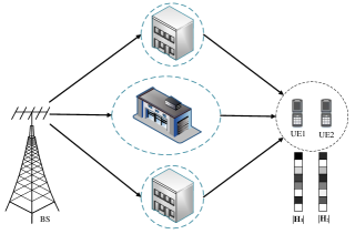
Figure 1: Illustration of the system model. The BS and the two nearby UEs are equipped with ULAs with $N_{t}$ transmit and $N_{r}$ receive antennas, respectively.

2.2 Conventional DL-based Digital CSI Feedback Process

Here, the UE is assumed to know the perfect CSI, and only the CSI feedback is considered. For most DL-based CSI feedback methods, once the UE obtains the channel matrix H, an NN is first used to compress the CSI, which directly outputs the measurement vectors with 32-bit floating point numbers. Then, the following quantization module generates the bitstreams, which are fed back to the BS immediately. Subsequently, the BS reconstructs the CSI from the measurement vectors disturbed by the quantization noise. The entire process can be expressed as

$$\hat{\textbf{H}}=f_{\rm de}(\mathcal{D}(\mathcal{Q}(f_{\rm en}(\mathbf{H},\Theta_{\rm en}))),\Theta_{\rm de}),$$ (5)

where $f_{\rm en}(\cdot)$ and $f_{\rm de}(\cdot)$ represent the DL-based compression (encoder) and decompression (decoder) operations at the UE and the BS, respectively; $\mathcal{Q}$ and $\mathcal{D}$ denote the quantization and the dequantization operations, respectively; $\Theta_{\rm en}$ and $\Theta_{\rm de}$ are the parameters at the NN-based encoder at the UE and the decoder at the BS, respectively. The final feedback overhead, that is, the bitstream length, is derived through the compression ratio and the number of quantization bits as

$$N_{\rm bits}=L\times\gamma\times B,$$ (6)

where $L$ is the original dimension of the CSI, $\gamma$ is the compression ratio, and $B$ denotes the number of quantization bits.

The entire process is optimized by an end-to-end approach to minimize the loss function via updating the NN parameters. The most widely used loss function in CSI feedback is the mean-squared error (MSE):

$$(\hat{\Theta}_{1},\hat{\Theta}_{2})=\mathop{\arg\min}_{\Theta_{1},\Theta_{2}}\ \ \|\mathbf{H}-f_{\rm de}(\mathcal{D}(\mathcal{Q}(f_{\rm en}(\mathbf{H},\Theta_{1}))),\Theta_{2})\|_{2}^{2},$$ (7)

where ${\|\cdot\|}_{2}$ represents the Euclidean norm.

Following [41], to evaluate the difference between the original and the reconstructed CSI at the BS, the normalized MSE (NMSE) is used as follows:

$${\rm NMSE}=\mathbb{E}\bigg{\{}\frac{{\|\hat{\textbf{H}}-\textbf{H}\|}_{2}^{2}}{{\|\textbf{H}\|}_{2}^{2}}\bigg{\}},$$ (8)

where $\mathbb{E}(\cdot)$ represents the expectation.

3 DL-based CSI Feedback and Cooperative Recovery

In this section, the scenario with two nearby UEs, which share some reflection or diffraction media and are correlated in the CSI magnitude, is considered. Unlike the conventional cooperation strategy, which is enabled by D2D communications, no extra operations are performed at the UE in our DL-based cooperation strategy. The key idea is to reduce the overhead wasted by repeatedly feeding back the CSI information shared by the nearby UEs. After introducing our cooperation strategy, the NN modules in CoCsiNet are presented.

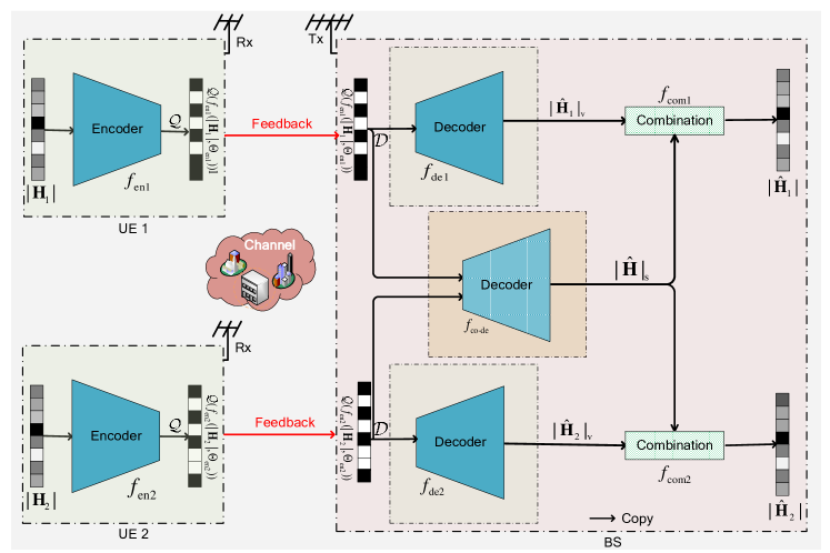
Figure 2: Illustration of the cooperative NN framework for two nearby UEs that includes two encoders and three decoders, that is, two individual decoders and one shared decoder. The encoders at the UE generate the bitstream and then feed back the bitstreams via the uplink channel. The decoders at the BS recover the shared CSI information and individual information from the feedback bitstreams by using the FC layers.

Algorithm 1 The proposed CoCsiNet for CSI magnitude feedback

0:  CSI magnitude vectors at the UEs: $|\mathbf{H}_{1}|$, $|\mathbf{H}_{2}|$;

0:  Reconstructed CSI magnitude vectors at the BS: $|\hat{\textbf{H}}_{1}|$, $|\hat{\textbf{H}}_{2}|$;

1:  Compresses and quantize CSI:   ${\bf s}_{1}=\mathcal{Q}\big{(}f_{\rm en1}(|\mathbf{H}_{1}|,\Theta_{\rm en1})\big{)}$, ${\bf s}_{2}=\mathcal{Q}\big{(}f_{\rm en2}(|\mathbf{H}_{2}|,\Theta_{\rm en2})\big{)}$

2:  UEs feedback ${\bf s}_{1}$ and ${\bf s}_{2}$ to the BS

3:  Reconstruct individual information:   $|\hat{\textbf{H}}_{1}|_{\rm v}=f_{\rm de1}\Big{(}\mathcal{D}({\bf s}_{1}),\Theta_{\rm de1}\Big{)}$, $|\hat{\textbf{H}}_{2}|_{\rm v}=f_{\rm de2}\Big{(}\mathcal{D}({\bf s}_{2}),\Theta_{\rm de2}\Big{)}$

4:  Reconstruct shared information:   $|\hat{\textbf{H}}|_{\rm s}=f_{\rm co-de}\Big{(}\mathcal{D}({\bf s}_{1}),\mathcal{D}({\bf s}_{2}),\Theta_{\rm co-de}\Big{)}$

5:  Combine the individual and shared information:  $|\hat{\textbf{H}}_{1}|=f_{\rm com1}(|\hat{\textbf{H}}_{1}|_{\rm v},|\hat{\textbf{H}}|_{\rm s},\Theta_{\rm com1})$,   $|\hat{\textbf{H}}_{2}|=f_{\rm com2}(|\hat{\textbf{H}}_{2}|_{\rm v},|\hat{\textbf{H}}|_{\rm s},\Theta_{\rm com2})$

3.1 Cooperation Strategy

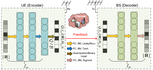
Figure 3: Illustration of the NN architecture, which includes the encoder and the decoder. The encoder at the UE generates the bitstream by using the FC layers and the quantization or binary layer, and then feeds back the bitstreams via the uplink channel. The decoder at the BS recovers the CSI from the feedback bitstreams by using the FC layers.

Fig. 1 shows that UEs can share the same scatterers and similar deterministic multipath components if they are nearby. According to [33, 36, 42, 43, 38], the channel parameters of these two nearby UEs are similar, and the magnitude of the CSI in the angular domain is correlated. However, no correlation exists in the CSI phase. To exploit the shared common sparsity structures in the CSI, the sparse vector of CSI is divided into two parts (as in [36]): the commonly shared and the individual sparse representation vectors. Inspired by this work, the CSI magnitude $|\textbf{H}_{i}|$ information of the $i$-th UE is divided into two parts: shared by nearby UE and owned by individual UE.

To exploit this characteristic, the autoencoder-based NN framework should be modified. However, no modifications are made to the encoder framework of the UE, that is, the NN architectures and the parameter number are maintained because the UE has limited computation power and storage capability. The feedback bitstreams of two UEs are obtained by

$${\bf s}_{1}=\mathcal{Q}\big{(}f_{\rm en1}(|\mathbf{H}_{1}|,\Theta_{\rm en1})\big{)},$$ (9)

$${\bf s}_{2}=\mathcal{Q}\big{(}f_{\rm en2}(|\mathbf{H}_{2}|,\Theta_{\rm en2})\big{)},$$ (10)

where $f_{\rm en1}(\cdot)$ and $f_{\rm en2}(\cdot)$ are the encoder modules at the two UE; $\Theta_{\rm en1}$ and $\Theta_{\rm en2}$ are the NN parameters of the two encoder modules.

Only the NN framework at the BS is modified. The decoder at the BS has two modules, shared and individual modules, that recover the vectors containing shared and individual information, respectively. For the case of two nearby UEs, the BS has three decoder modules, namely, a shared decoder and two individual decoders, as illustrated in Fig. 2. Given that the shared information of nearby UEs is the same, the first decoder module can be used for the two nearby UEs to reconstruct the shared information $|\hat{\textbf{H}}|_{\rm s}$ as

$$|\hat{\textbf{H}}|_{\rm s}=f_{\rm co-de}\big{(}\mathcal{D}({\bf s}_{1}),\mathcal{D}({\bf s}_{2}),\Theta_{\rm co-de}\big{)},$$ (11)

where $\Theta_{\rm co-de}$ is the parameter of shared decoder $f_{\rm co-de}(\cdot)$. Then, two individual decoders reconstruct the corresponding individual CSI information, $|\hat{\textbf{H}}_{1}|_{\rm v}$ and $|\hat{\textbf{H}}_{2}|_{\rm v}$, as

$$|\hat{\textbf{H}}_{1}|_{\rm v}=f_{\rm de1}\Big{(}\mathcal{D}({\bf s}_{1}),\Theta_{\rm de1}\Big{)}$$ (12)

$$|\hat{\textbf{H}}_{2}|_{\rm v}=f_{\rm de2}\Big{(}\mathcal{D}({\bf s}_{2}),\Theta_{\rm de2}\Big{)}$$ (13)

where $\Theta_{\rm de1}$ and $\Theta_{\rm de2}$ represent the parameters of the two individual decoders, that is, $f_{\rm de1}(\cdot)$ and $f_{\rm de2}(\cdot)$. Subsequently, two modules combine the information shared by nearby UE and owned by individual UE by using FC layers as

$$|\hat{\textbf{H}}_{1}|=f_{\rm com1}(|\hat{\textbf{H}}_{1}|_{\rm v},|\hat{\textbf{H}}|_{\rm s},\Theta_{\rm com1}),$$ (14)

$$|\hat{\textbf{H}}_{2}|=f_{\rm com2}(|\hat{\textbf{H}}_{2}|_{\rm v},|\hat{\textbf{H}}|_{\rm s},\Theta_{\rm com2}),$$ (15)

where $f_{\rm com1}(\cdot)$ and $f_{\rm com2}(\cdot)$ are the combination modules at the two nearby UE; $\Theta_{\rm com1}$ and $\Theta_{\rm com2}$ are the NN parameters of these two modules; $|\hat{\textbf{H}}_{1}|$ and $|\hat{\textbf{H}}_{2}|$ are the final reconstructed magnitude matrices of the CSI.

Fig. 2 shows the entire cooperative CSI feedback framework , which consists of the encoders at the UE and the decoders at the BS. Details of the encoder and decoder modules are provided subsequently. At the UE, the two encoders generate the bits via the FC layers and the binary (or quantization) layer. Once the bitstreams are generated, they feed back the bits via uplink transmission. Then, the shared decoder at the BS recovers the shared CSI information from the feedback of the two nearby UE. At the same time, the individual decoders recover the individual CSI information for the two UEs. The final CSI magnitude matrix is the combination of the recovered shared and individual CSI magnitude information. The co-decoder network architecture is similar to that of the individual decoder except that the input of the co-decoder is the feedback of all the cooperative UEs. The combination network consists of an FC layer with $N_{\rm r}N_{\rm t}$ neurons and Sigmoid activation function. The proposed CoCsiNet contains explicit and implicit cooperation. Explicit cooperation is that the decoder at the BS jointly recovers the CSI from the feedback of nearby UEs. Implicit cooperation is in the compression at the encoders. Different from the NNs without cooperation, which have to feed back the shared CSI information by the UE repeatedly, the encoders at the CoCsiNet cooperatively feed the shared CSI information back through the end-to-end learning.

The training of the two nearby UEs should be performed together, thereby enabling CoCsiNet to extract and recover the shared CSI information. Therefore, the proposed CoCsiNet is directly trained using a one-step end-to-end learning approach. Training loss function ${\rm MSE}_{\rm CoCsiNet}$ is the overall MSE of the two UE as

$${\rm MSE}_{\rm CoCsiNet}=\left\||\mathbf{H}_{1}|-\hat{|\mathbf{H}}_{1}|\right\|_{2}^{2}+\left\||\mathbf{H}_{2}|-\hat{|\mathbf{H}}_{2}|\right\|_{2}^{2}.$$ (16)

Given that the encoder of the CoCsiNet at the UE is the same as many existing feedback frameworks without UE cooperation, the NN parameter number and floating-point operations do not increase. Although an extra shared decoder exists at the BS, which increases the NN complexity, slight effect can be exerted on the running speed of the CSI reconstruction because the computation power is not limited at the BS, and three decoders can run parallelly.

The proposed CoCsiNet can be easily extended to the scenario with more UEs. Each UE is still equipped with an encoder. Assuming that the nearby UE number is $K$, at the BS, a shared decoder reconstructs the shared information based on the feedback from $K$ UEs. $K$ individual decoders reconstruct their corresponding individual information. Finally, combination modules mix the shared and individual information to produce the final CSI of $K$ UEs.

3.2 NN Modules in the CoCsiNet

In this part, the baseline NN architecture used in this work is first introduced. Then, the binarization operation, which generates the bitstreams and can be regarded as an extension of the one-bit quantization, is described. Finally, a phase strategy called MDPF is proposed.

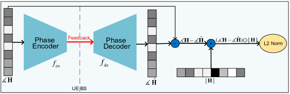
Figure 4: Illustration of MDPF-1. During the training, the loss function is the weighted MSE function dependent on the CSI magnitude, which then introduces statistical CSI magnitude information to the NNs. The quantization module following the encoder is neglected in this figure.

3.2.1 Baseline NN Architecture

Fig. 3 shows the NN architecture, including an encoder and a decoder. The encoder at the UE is composed of three FC layers followed by three batch normalization (BN) layers. The activation function of the first two BN layers is the LeakyReLu function, which assigns a non-zero slope to the negative part compared with the standard ReLu activation function, as

$${\rm LeakyReLu}(x)=\begin{cases}x&{\quad x\geq 0}\\ ax&{\quad x<0}\end{cases},$$ (17)

where $a$ is a small number. The activation function of the last BN layers is a $\tanh$ function, which aims to generate the numbers in the continuous interval $[-1,1]$ as

$$\tanh(x)=\frac{e^{x}-e^{-x}}{e^{x}+e^{-x}}.$$ (18)

The last layer at the encoder is the quantization or the previously mentioned binary layer. The decoder at the BS also contains three FC layers . Unlike the NN layers at the encoder, the neuron number of the last FC layer here is $N_{r}\times N_{t}$, and the last BN layer employs the Sigmoid function to normalize the outputs into $[0,1]$.

If the UE is equipped with multiple antennas, then an LSTM architecture is added to the last layers at the decoder to exploit the correlation among different antennas at the same UE, like the architecture in [23]. The LSTM architecture is widely used in time-varying scenarios to extract and utilize the time correlation, such as CsiNet-LSTM [23]. LSTM is designed for sequence data. In the sequence data, a correlation exists between the adjacent “frames.” This correlation involves not only the time correlation but also others, such as frequency correlation and spatial correlation. Therefore, in this work, LSTMs are used to extract and exploit the correlations between nearby antennas. The extra LSTM at the decoder can well reconstruct the CSI because this NN architecture has inherent memory cells and can keep the previously extracted information for a long period for later reconstruction. Further details about the LSTM module can be found in [44].

In [21], after the FC layers at the decoder, several convolutional layer-based RefineNet modules are added to refine the initial reconstructed CSI. Here, the LSTM layers can also be regarded as a module that refines the initial output of the baseline decoder by using the antenna correlation. Specifically, once the baseline decoder outputs the initial reconstructed CSI ${\hat{\rm{\textbf{H}}}}_{i}^{{}^{\prime}}=[{\hat{\rm{\textbf{h}}}}_{i,1}^{{}^{\prime}},{\hat{\rm{\textbf{h}}}}_{i,2}^{{}^{\prime}},\cdot\cdot\cdot,{\hat{\rm{\textbf{h}}}}_{i,N_{r}}^{{}^{\prime}}]^{\rm T}\in\mathbb{R}^{N_{r}\times N_{t}}$, the initial CSI of the $i$-th UE is divided into $N_{r}$ vectors, and each vector is then used as an input to the three stacked LSTM layers. The outputs of $N_{r}$ LSTM modules are concatenated to generate the final reconstructed $\hat{\rm\textbf{H}}_{i}$. The entire NN is trained via an end-to-end approach, and the loss function used in the CSI magnitude feedback is the MSE function.

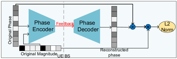
Figure 5: Illustration of MDPF-2. The CSI magnitude is also input to the encoder and the final loss function of the CSI phase feedback NNs is the weighted MSE function dependent on the instant CSI magnitude.

3.2.2 Binarization Operation

Conventional DL-based methods, which can be regarded as DL-based CS algorithms, have two main operations, namely, compression and quantization. From the perspective of the machine learning domain, the first operation aims to generate the latent representative vectors of the original CSI or extract the features of the original CSI. The quantization operation quantizes the features to decrease feedback overhead.

Furthermore, the binary representation can be used to generate the bitstreams [29]. To an extent, this binary presentation-based CSI feedback can be regarded as a codebook-based data-driven feedback strategy. Unlike the previous methods on codebook design, the NN-based encoder, including the binary layer, can be regarded as the module that generates the codebook indices, which are composed of a set of $\{-1,1\}$. Correspondingly, the NN-based decoder recovers the CSI by using the codebook indices. According to [45], the binarization operation contains two main steps.

• The neuron number of the last FC layer at the encoder is set the same as the desired length of the feedback bits. To generate the numbers in the continuous interval $[-1,1]$, the activation function of the BN following the last FC layer is $\rm{tanh(\cdot)}$.

• The real-valued representation is then taken as the input to generate a discrete output in the $\{-1,1\}$ set by binarization function $b(\cdot)$ of $x\in[-1,1]$, which is defined as

  $$b(x)=x+\epsilon,$$ (19)

  $$\epsilon=\begin{cases}1-x&{\rm{with\quad probability}\quad\frac{1+x}{2}},\\ -x-1&{\rm{with\quad probability}\quad\frac{1-x}{2}},\end{cases}$$ (20)

  where $\epsilon$ denotes the quantization noise, and $\mathbb{E}(\epsilon)=0$.

Given that the second step is nondifferentiable, the gradient of this step is set as one to backpropagate gradients through this operation, that is, binary layer $\mathcal{B}$.

3.2.3 NN for Phase Feedback

Unlike the CSI magnitude, which is sparse due to limited paths, the phase matrix of the CSI is not sparse at all. If the phase information is fed back by the same method as magnitude feedback, then too much useless information must be relayed. The feedback bits corresponding to the CSI with a small magnitude have minimal useful information and waste resources. If this information can be dropped during the feedback process, the feedback overhead will be efficiently exploited, and the feedback performance can be greatly improved.

In [24], a magnitude dependent phase quantization strategy is proposed, where CSI coefficients with large magnitudes adopt finer phase quantization, and vice versa. The more important the CSI phase is, the more bits can be allocated. In [46], an extra NN is introduced to allocate the quantization bits. Inspired by the above work, two magnitude-dependent strategies are adopted for the CSI phase feedback, which are dependent on the statistical and the instant CSI magnitudes.

MDPF-1

Unlike the previous work focusing on the allocation of quantization bits, the NN focuses on coefficients with large magnitudes by modifying the loss function in the MDPF-1. In the above-mentioned magnitude feedback, the loss function is the naive MSE function. The MSE loss function equally treats each coefficient in the matrix and narrows the gap between the ground truth and the prediction. This naive loss function does not consider the importance of the phase coefficient. Therefore, as illustrated in Fig. 4, the MSE loss function is modified by introducing important information, that is, the statistical magnitude information as

$$MSE_{\rm phase}=\|(\measuredangle\mathbf{H}-\measuredangle\hat{\mathbf{H}})\odot|\mathbf{H}|\|_{2}^{2},$$ (21)

where $\measuredangle\mathbf{H}$ denotes the original phase of the CSI in radians, $\measuredangle\hat{\mathbf{H}}$ is the predicted phase, $|\mathbf{H}|$ is the corresponding CSI magnitude, and $\odot$ represents the Hadamard product.

The NNs used in the MDPF-1 are similar to the baseline NN architecture in the magnitude feedback. During the parameter update, large errors have much influence on MSE loss because MSE squares the errors before they are averaged [47]. Given that the importance of the phase is decided by the corresponding CSI magnitude, the larger the magnitude is, the larger the MSE. By adding the magnitude information to the loss function of the phase feedback, the parameter update can favor the phase coefficients with large magnitudes. Given that the instant CSI magnitude is not an input of this network during the test, the proposed method compresses and feeds back the CSI phase using the statistical CSI magnitude information, which is learned during the training by introducing the instant CSI magnitude to the loss function.

MDPF-2

Different from MDPF-1, where the instant CSI magnitude is not as input of this network and only the statistical CSI magnitude information is used, the instant CSI magnitude is input to the encoder in MDPF-2, as shown in Fig. 5. The other parts, including the loss function, the NN architecture, and the training strategy, are all the same as those in MDPF-1.

4 Simulation Results and Discussions

In this section, a numerical simulation is conducted to evaluate the feedback performance of our proposed methods. First, the simulation setting, including the channel parameters, the NN architecture details, and the NN training details, is introduced. Then, the quantization and binarization performance are compared. Numerical simulation is conducted to demonstrate the superiority of the proposed methods in Section 3, namely, the extra LSTM and the MDPF strategy. Finally, the proposed cooperation-based NNs, that is, CoCsiNet, is compared with the NNs, ignoring the CSI correlation between the nearby UEs. According to [27], insight into the cooperative CSI feedback is obtained via NN parameter visualization.

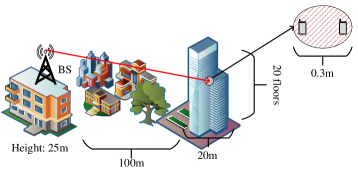
Figure 6: Illustration of the simulation environment of the dataset generated by QuaDRiGa software

4.1 Parameter Setting

4.1.1 Channel Generation

To evaluate the proposed CoCsiNet, two different channel datasets generated by ourselves and public software, are used. First, channels of the urban microcell are generated using the 3GPP spatial channel model (SCM) [39]. Following the setting in [36], the frequency of the downlink is 2.17 GHz. The inter antenna spacing is half wavelength, that is, $d=c/(2f_{0})$, where $c$ is the light speed and $f_{0}$ = 2 GHz in carrier frequency. $N_{c}=3,4,5,6$ random scattering clusters (paths) ranging from $-\pi/2$ to $\pi/2$ exist. The number of BS antennas is 64 or 256, and the number of UE antennas is 1 or 4. Given that the UE are assumed to be nearby, such as the stadium scenario, the nearby UE’s CSI shares the most scattering clusters and has similar path loss. Specifically, the channel parameters of the first UE, namely, AoA, AoD, and gain, are first randomly set. Then, the channel parameters of the second UE are generated by adding small random values to those of the first UE. A total of 100,000 pairs of CSI samples are generated by MATLAB.

Instead of generating a database by adding a small random value to the channel parameter, the second dataset is generated by QuaDRiGa software [48], satisfying 3GPP TR 38.901 v15.0.0 [49]). The urban microcell (UMi) scenario with non line-of-sight (NLOS) paths, i.e., 3GPP_38.901_UMi_NLOS scenario, is considered. The simulation environment is shown in Fig. 6. The height of the BS, with 256 transmit antennas, is 25 m. The building with 20 floors is 100 m away from the BS. The UE is located in a $\rm 20\quad m\times 20\quad m$ area and randomly located on the 20 floors. The height of each floor is 3 m and the UE height is 1.5 m. A total of 10,000 groups of CSI are randomly generated. As mentioned in [2], the device density grows to hundred(s) per cubic meter in the future, where the users are tens of centimeters apart. Therefore, each group has two or four UEs, and the distance between any two is less than 0.3 m.

TABLE I: The detailed architecture of the proposed NNs

	Layer name	Output size	Activation function
Encoder (UE)	Input Layer	$N_{r}\times N_{t}$	None
	Reshape1	$N_{r}N_{t}\times 1$	None
	FC1+BN1	$2N_{r}N_{t}\times 1$	LeakyReLu
	FC2+BN2	$2N_{r}N_{t}\times 1$	LeakyReLu
	FC3+BN3	$N_{\rm{bits}}/B$ * or $N_{\rm{bits}}\times 1$	Tanh
	Quantization or Binary layer	$N_{\rm{bits}}\times 1$	None
Decoder (BS)	FC4+BN4	$4N_{r}N_{t}\times 1$	LeakyReLu
	FC5+BN5	$4N_{r}N_{t}\times 1$	LeakyReLu
	FC6+BN6	$N_{r}N_{t}\times 1$	Sigmoid / Tanh **
	Reshape2	$N_{r}\times N_{t}$	None
	LSTM1	$N_{r}\times N_{t}$	-
	LSTM2	$N_{r}\times N_{t}$	-
	LSTM3	$N_{r}\times N_{t}$	-

• $B$ represents the number of quantization bits.

• If the decoder is used to recover CSI magnitude, we choose the Sigmoid function. If the decoder is used to recover CSI phase, we choose the Tanh function.

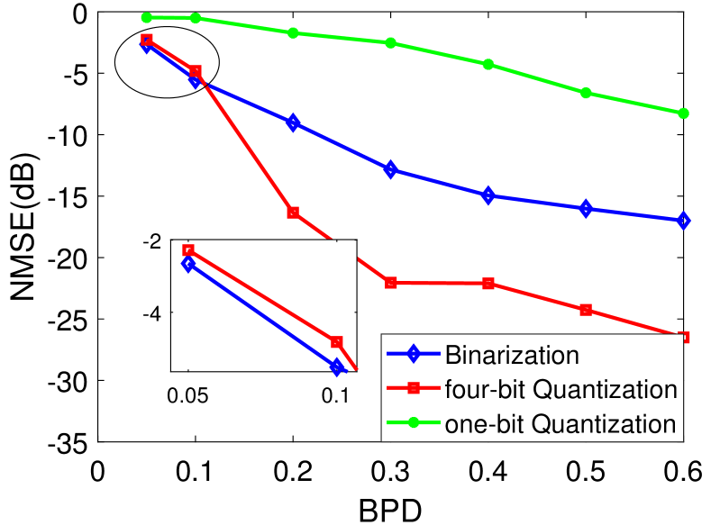
Figure 7: NMSE (dB) performance comparison of CSI magnitude feedback between four and one-bit quantization, and binarization operation under different BPD. The BS is equipped with 256 antennas, and the UE has a single antenna. The first SCM dataset is adopted, and the channel path number is $N_{c}=5$.

The datasets are randomly divided into training, validation, and test datasets with 70%, 10%, and 20% samples, respectively. During the training, the first dataset is used to update the NN parameters, and the second is used to avoid over-fitting. In this work, early stopping is adopted to avoid overfitting as soon as the performance on the validation dataset decreases. Furthermore, bit per dimension (BPD) is used here to describe the feedback overhead, which is widely used in the image compression domain and defined as

$${\rm BPD}=\frac{N_{\rm bits}}{N_{\rm r}N_{\rm t}}.$$ (22)

4.1.2 NN Architecture

In Section 3.2.1, the NN architecture is briefly introduced. In this part, the details of the NN architecture and the training are provided. Given that our main contribution is not designing NN architectures for CSI feedback, only the standard FC, BN, and LSTM layers are used. The UE and the BS have three FC layers. Considering sufficient computation power at the BS, the FC layers at the BS are twice wider than those at the UE. Table I shows the parameters of the proposed NNs , including the neuron numbers of the FC layers and the activation function.

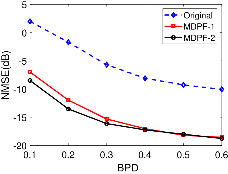
Figure 8: NMSE (dB) performance of the CSI phase feedback. The BS is equipped with 256 antennas, the UE is equipped with a single antenna, the first SCM dataset is adopted, and the channel path number is $N_{c}=3$.

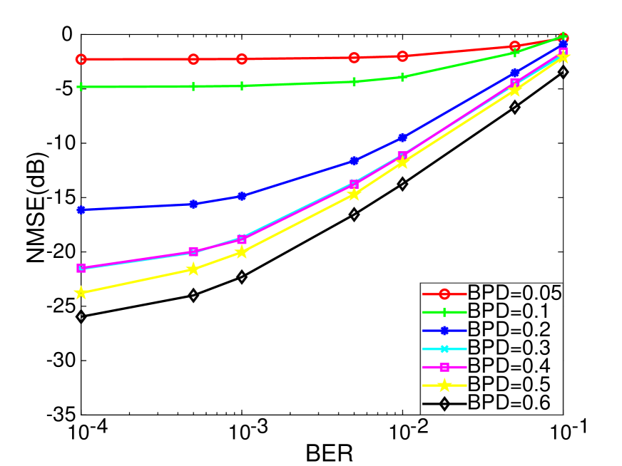
Figure 9: NMSE (dB) performance of CSI feedback with imperfect uplink transmission. The scenario is considered where the BS is equipped with 256 antennas, the UE is with a single antenna, the first SCM dataset is adopted, and the channel path number is $N_{c}=5$. The BER is from 0.1 to 0.0001.

Simulation is run on TensorLayer 1.11.0 and conducted on one NVIDIA DGX-1 station. The batch size is set to 200, the learning rate is 0.001, and the epoch is 1,000. During the training, the adaptive moment estimation is used to optimize the loss function.

4.2 Performance of NN-based CSI Magnitude Feedback

In this part, the performance of the NN-based CSI magnitude feedback with the first SCM dataset is evaluated.

First, the two main methods of generating bitstreams, namely, quantization and binary representation, are compared. The single-user scenario, where the BS is equipped with 256 antennas and the UE has a single antenna, is considered. The number of the quantization bits, $B$, is set as 4, which is proven the best through simulation in[25]. The BPD-NMSE tradeoffs achieved by the quantization and binarization are plotted in Fig. 7.

To an extent, the binarization operation can be regarded as a special case of quantization with $B=1$. Unlike the general quantization, as in (20), the binarization operation introduces quantization noise $\epsilon$ with a zero-mean property, thereby making $b(x)$ an unbiased estimator for soft value $x$, that is, $\mathbb{E}_{\epsilon}[b(x)|x]=x$ [29]. The binarization operation and the common one-bit quantization are also compared in Fig. 7. The former outperforms the latter by a large margin, indicating the importance of zero-mean $\epsilon$. The performance of the quantization operation is better than that of the binarization operation for most scenarios, except when the BPD is very low, that is, the feedback overhead is extremely limited.

Fig. 9 illustrates the robustness of the proposed NNs by using the quantization operation to the imperfect uplink transmission. The scenario, where the BS is equipped with 256 antennas, the UE has a single antenna, and the channel path number is $N_{c}=5$, is considered. Unlike most works that directly add noise to the codewords and use signal-to-noise ratio to describe the uplink condition [27], the bit-error ratio (BER) is used to denote the feedback condition because the focus is now on the digital CSI feedback rather than the analog one. During the test phase, the errors are introduced by the bit-wise exclusive-or between feedback bits and $1$ at a predefined probability, that is, BER. Clearly, the NN performance worsens as the BER increases. However, the feedback with a high BPD is more sensitive to the BER, that is, the uplink transmission condition, than that with a low BPD. Fig. 9 indicates that for the feedback with a low BPD, namely, 0.05 and 0.1, no degradation in feedback accuracy is observed if the BER is lower than 0.005. For the feedback with a high BPD, namely, 0.4, 0.5, and 0.6, even the BER is very low (e.g., 0.0001), performance degradation is still observed. Therefore, the feedback with a high BPD is more sensitive to the uplink condition than that with a low BPD.

TABLE II: NMSE ($dB$) performance comparison between the FCNN and the LSTM.

$N_{c}$	3	4	5	6
LSTM *	-24.84	-20.98	-20.82	-18.94
FCNN **	-21.95	-18.75	-18.31	-16.52

• LSTM represents the NNs with LSTM modules.

• FCNN represents the FC NNs.

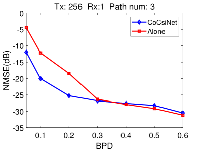
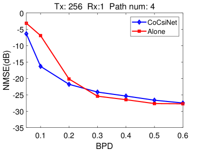
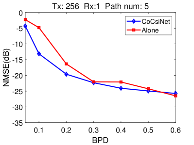
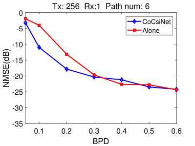
Figure 10: NMSE (dB) performance comparison between the CoCsiNet and the NNs without cooperation given 256 antennas at the BS and a single antenna at the UE. The first SCM dataset is adopted, and the channel path number is $N_{c}=3,4,5,6$.

If the UE is equipped with multiple antennas, the extra LSTM module is added after the FC layers of the decoder to well extract the correlation between the nearby antennas at the UE. Here,a scenario, where the BS and the UE are equipped with 64 and 4 antennas, is considered. Table II compares the feedback performance of the FC NNs and the NNs with LSTM modules when the BPD is 0.3. The table displays the improvement of the feedback accuracy for different path numbers due to the extra LSTM modules.

4.3 Performance of MDPF NNs

In this part, the performance of the proposed MDPF NNs is evaluated with the first SCM dataset, where the magnitude information is added to the loss function of the phase feedback.

Different from the compression and feedback of the CSI magnitude, the compression of the CSI phase is dependent on the CSI magnitude. Therefore, when evaluating the feedback accuracy of the CSI phase, the NMSE between the original and the reconstructed CSI phase is not directly calculated, but the NMSE between the original and the reconstructed complex CSI, that is,

$${\rm NMSE}={\rm E}\bigg{\{}\frac{\|(\measuredangle\mathbf{H}-\measuredangle\hat{\mathbf{H}})\odot|\mathbf{H}|\|_{2}^{2}}{{\|\textbf{H}\|}_{2}^{2}}\bigg{\}}.$$ (23)

The scenario, where the BS is equipped with 256 antennas, the UE is equipped with a single antenna, and the channel path number is $N_{c}=3$, is considered. Fig. 8 plots the BPD-NMSE tradeoffs achieved by MDPF-1, MDPF-2, and the naive phase feedback method. When the BPD is very low, the NMSE of the original phase feedback method exceeds 0 dB, which means that slight useful information about the CSI phase is fed back because the NNs do not know which information is significant, only attempt to feed back all the phase information, and require many feedback bits. A 8.93 dB improvement is achieved by MDPF-1 and MDPF-2 when the BPD is 0.5. MDPF-2, which exploits instant CSI magnitude information, outperforms MDPF-2, specifically when the BPD is low. As the BPD increases, the gap becomes smaller, because feedback bit is enough for all required phase information for MDPF-1 and MDPF-2.

To exploit the correlation in the CSI magnitude, the phase and the magnitude of the CSI are fed back separately, thereby leading to a bit-allocation problem in the phase and magnitude feedback. The unoptimized allocation strategy leads to a great decrease in CSI feedback accuracy. A similar issue has been also mentioned in [46], which is regarded as an important direction in the future. To the best of our knowledge, no reasonable allocation strategy is in the existing works. Therefore, the best bit-allocation strategy is specifically through an exhaustive search based on extensive simulation. How to allocate bits adaptively will be considered in our future work because the goal of this work is to show the performance improvement achieved by exploiting the UE correlation.

4.4 Performance of Cooperative CSI Feedback

In this part, the performance of the proposed cooperative CSI feedback NNs, CoCsiNet, using the two datasets is evaluated, and the mechanism is explained via NN parameter visualization.

4.4.1 Comparison between CoCsiNet, CS, and NNs without cooperation

Fig. 10 compares the performance of the CoCsiNet and the NNs without cooperation with the first SCM dataset when the BS has 256 antennas, the UE has a single-receiver antenna, and the channel path number is $N_{c}=3,4,5,6$. When the BPD is low, the proposed CoCsiNet outperforms the original one by a large margin because the feedback information of the single UE is extremely few to recover the CSI accurately for the decoder at the BS when the BPD is low, that is, the feedback overhead is extremely constrained. Therefore, in this scenario, the shared information does not need to be fed back repeatedly if the two UEs can feed back the CSI via cooperation. However, when the BPD exceeds 0.3, a small gap exists between the two methods, because the feedback information of the single UE is enough to recover the CSI accurately for the decoder at the BS.

Fig. 11 compares the feedback performance of the CoCsiNet with LSTM modules and the NNs without cooperation with the first SCM dataset when the BS has 64 antennas and the UE has 4 antennas at the UE, respectively. The BPD is 0.05 or 0.10, and the channel path number is $N_{c}=3,4,5,6$. For the scenario with low BPD, CoCsiNet outperforms the NNs without cooperation by a large margin. When the BPD is 0.05, the gap between the CoCsiNet and the NNs without cooperation decreases as the channel path number increases. By contrast, when the BPD is 0.10, the gap increases as the channel path number increases. For extremely low BPDs, such as 0.05, the feedback bits are insufficient for the CoCsiNet. Therefore, if many channel paths exist and further information is needed to be fed back, CoCsiNet cannot handle this scenario, thereby narrowing the performance gap.

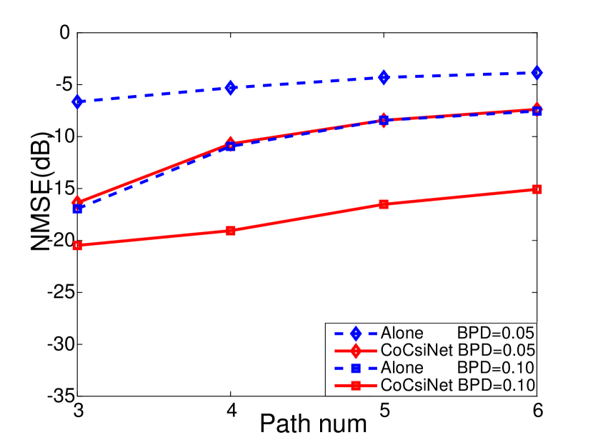
Figure 11: NMSE (dB) performance comparison between the CoCsiNet with LSTM modules and the NNs without cooperation with the first SCM dataset when the BS has 64 antennas and the UE has 4 antennas, respectively, the BPD is 0.05 or 0.10, and the channel path number is $N_{c}=3,4,5,6$.

To make the validation of the proposed CoCsiNet more convincing, the cooperation framework is evaluated using the second channel dataset, which satisfies 3GPP TR 38.901 v15.0.0. Different from the above comparison, which just considers the baseline NN architecture, more benchmarks are considered to ensure that the performance gain achieved by CoCsiNet is not due to the NN complexity, as shown in Fig. 12.

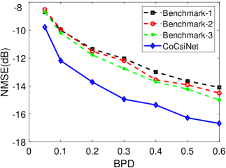
Figure 12: NMSE (dB) performance comparison between the CoCsiNet and the NNs without cooperationgiven 256 antennas at the BS, a single antenna at the UE, and the channel model of 3GPP_38.901_UMi_NLOS

Benchmark-1 represents the baseline architecture used in Fig. 10. Benchmark-2 represents the network architecture whose neuron number of the FC layers at the decoder is twice that in the baseline architecture. Benchmark-3 is similar to the architecture of the proposed CoCsiNet. With some modifications, where the input of the co-decoder is the feedback from the cooperative UE, the input of the co-decoder here is the feedback of one UE. According to the figure, the proposed CoCsiNet outperforms all benchmarks, which further demonstrates the importance of exploiting the correlation in the CSI magnitude of nearby UEs. Different from the simulation results in the first dataset, the proposed CoCsiNet always outperforms the NNs without cooperation no matter what the BPD is. The performance gap may be related to channel complexity because different datasets show dissimilar simulation results. The gap increases with the channel complexity. For a simple channel, the gap is negligible when the BPD is high.

TABLE III: NMSE($\rm dB$) performance comparison (3GPP_38.901_UMi_NLOS scenario).

	0.05	0.1	0.2	0.3	0.4	0.5	0.6	0.7	0.8	0.9	1.0	2.0
CS	0.65	0.76	0.74	0.60	0.38	0.13	-0.12	-0.46	-0.85	-1.26	-1.66	-6.43
Alone	-8.71	-10.01	-11.36	-12.04	-13.00	-13.65	-14.10	/	/	/	/	/
CoCsiNet-2UE	-10.62	-11.31	-13.57	-14.98	-15.43	-15.82	-16.38	/	/	/	/	/
CoCsiNet-4UE	-9.79	-12.19	-13.72	-14.95	-15.36	-16.28	-16.68	/	/	/	/	/

The DL-based feedback methods are also compared with the CS-based method. Table III compares the NMSE performance. The CS problem is solved by the CVX toolbox. The CS-based method performs extremely poorly compared with the DL-based method, which is similar to the simulation result in [21] when the compression ratio is low. In this work, the compression ratio in the CS-based method is extremely low. For example, when the BPD is 0.1, the compression ratio is 1/40. The CSI is first compressed by 40 times and then discreted by a 4-bit uniform quantizer. CS may not handle this scenario because sparsity is the only prior information that it can exploit. Moreover, the CS reconstruction ignores the effects of codeword quantization.

Table III also compares CoCsiNet with different cooperative UE numbers. The four-user cooperative case performs slightly better than the two-UE case because the shared information occupies fewer feedback bits for each UE with more cooperative UE, An exception is that the two-user cooperation outperforms the four-user one when the BPD is 0.05 because during the network training, the NNs become more difficult to train with the increase of the UE number, especially when the BPD is low.

4.4.2 NN complexity analysis

The NNs in this work mainly consist of the FC layers. According to [50], the number of the FC layer’s floating point of operations (FLOPs) is approximately twice the network parameter number. Therefore, the parameter number is just calculated. Fig. 13 compares the parameter numbers. The increase in parameter number is very low compared with Benchmark 1. Moreover, the parameter number of the CoCsiNet is smaller than that of Benchmarks 2 and 3. Above all, in the proposed CoCsiNet, only two parts are added at the BS, namely, co-decoder and combination network, and no changes are made at the UE side. As mentioned in [27], the UE has limited resources (memory resources, computational units, and battery power) but the BS has sufficient resources. Therefore, the complexity increase of the proposed CoCsiNet can be ignored.

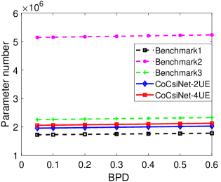
Figure 13: Comparison of the network parameter number of CoCsiNet and Benchmark-1, Benchmark-2, and Benchmark-3

Moreover, compared with the existing works [22], the NN complexity is much lower. The FLOP number of the proposed CoCsiNet is about 4 M, whereas that of the most existing works is over 10 M (more details can be found in Fig. 30 of [22] ). Therefore, the computational power requirement is low. To reduce the NN complexity further, some NN compression techniques, such as NN weight pruning and quantization [31], can be introduced to the proposed CoCsiNet. This is consideration out of the scope of this paper, and the interested readers are referred to [31].

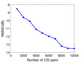
Figure 14: NMSE (dB) performance of CoCsiNet with different training samples given 256 antennas at the BS and a single antenna at the UE. The channel model is 3GPP_38.901_UMi_NLOS, and BPD is set as 0.2.

4.4.3 Effect of training sample number

DL-based algorithms learn knowledge from the training dataset by an end-to-end approach. Therefore, the algorithm performance is dependent on the training dataset. In this part, the effect of the training sample number is evaluated. Fig. 14 shows the NMSE performance of CoCsiNet with different training samples given 256 antennas at the BS and a single antenna at the UE. The channel model is 3GPP_38.901_UMi_NLOS, and BPD is set as 0.2. The feedback accuracy is improved with the training number. When the number is over 8,000, the performance improvement is less. The CSI collection may lead to extra communication overheads. However, the recent simulation results in [51] show that the uplink CSI samples can be directly used to train the downlink CSI feedback NNs. The UE does not need to collect and transmit the estimated downlink CSI to the BS for NN training. The BS can easily collect substantial uplink CSI samples for CSI feedback training. Therefore, the training samples are enough for the training of CoCsiNet in practical systems.

4.4.4 Generalization capabilities of the CoCsiNet

The reason behind the success achieved by the DL-based CSI feedback is that the NNs can learn the environment from the training dataset [27]. However, the ability of learning environment is a double-edged sword in communications. If the practical environment is remarkably different from the simulated one, the accuracy greatly drops for the DL-based applications in communications, which has been a great challenge for the deployment of the DL-based algorithms.

Fig. 15 shows the performance of the DL-based CSI feedback with cooperation with the second dataset generated by QuaDRiGa given a mismatch between the training and testing datasets. The UE in the training dataset is located at a $\rm 20\quad m\times 20\quad m$ area that is $100\quad m$ away from the BS, whereas the UE in the test dataset is located at a $20\quad m\times 20\quad m$ area that is $85\quad m$ away from the BS. The performance drops much given a mismatch.

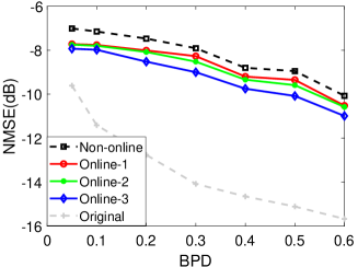
Figure 15: NMSE (dB) performance on the second dataset generated by QuaDRiGa given a mismatch between the training and test datasets. “Original” means no mismatch between the training and test datasets and “Non-online” means a mismatch between the training and test datasets. Online-1, Online-2,and Online-3 mean that the NNs are fine-tuned by the new datasets with 500, 1,000, and 1,500 samples, respectively.

As mentioned in [20], online training is necessary if the NNs work under the mismatched channel. Therefore, the trained NNs are fine-tuned using the new dataset with 500, 1,000, and 1,500 samples, which are much less than the original training dataset. A performance improvement occurs when the NNs are fine-tuned by the new dataset, and the performance improvement increases with the number of the samples used for fine-tuning. If the new dataset is enough, no performance drop is observed.

4.4.5 Cooperation mechanism

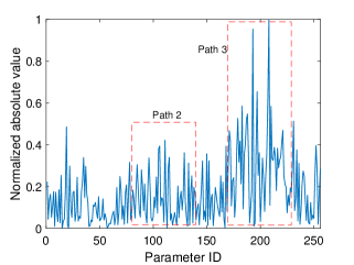
(a) Encoder parameter visualization for UE 1

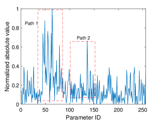
(b) Encoder parameter visualization for UE 2

Figure 16: Visualization of the normalized absolute value of the first FC layer at the encoders for the CoCsiNet when the first SCM dataset is adopted, and the BPD and channel path numbers $N_{c}$ are 0.05 and 3, respectively. The higher the absolute value is, the greater the attention that the NNs must pay.

The motivation of finding attention of the NNs by parameter visualization is NN pruning, where the small-weight connections are pruned [31]. The simulation results in [31] show that the feedback is closely dependent on the connections with high weights, which can be regarded as the areas of great interest. Through the parameter visualization, the authors in [27] finds the NNs in the CsiNet+ pay most attention to non-sparse areas. Table I shows that the dimension of the first FC layer at the encoder is $N_{r}N_{t}\times 2N_{r}N_{t}$. The mean absolute values of the weights along the second axis are calculated as

$${\bf W}_{i}=\sum_{j=1}^{2N_{r}N_{t}}|w_{i,j}|,$$ (24)

where $w_{i,j}$ represents the weight between the $i$-th input and $j$-th output neurons.

Fig. 16 plots the normalized mean absolute value ${\bf W}_{i}$ of two encoders for CoCsiNet, where the BS is equipped with 256 antennas, the UE is equipped with a single antenna, the first SCM dataset is adopted, and the BPD and the channel path number are set as 0.05 and 3, respectively. According to the statistical CSI, three paths are mainly located around three areas, corresponding to Parameter IDs 50, 125, and 200. Dotted rectangles are used to circle these areas, including the channel paths. The first and second encoders pay the most attention to the third and first path, respectively. The two encoders cooperatively feed back the information of the different paths. At the BS, they share their feedback information via the proposed shared decoder, and the feedback bits are not wasted to feed back the duplicate information. This situation explains why cooperation-based NNs can outperform NNs without cooperation .

4.4.6 Robustness to the degree of correlation

Given no correlation among the UEs, they do not share any information. Therefore, no performance gains can be achieved no matter what algorithms are adopted. The proposed method performs the same as that without exploiting correlation if the UEs’ CSI is independent. The degree of correlation may vary in practical systems. The key problem is how to make the proposed method robust to different degrees of correlation. If the NNs are trained with the CSI pairs with high correlation, the NNs cannot work well when the correlation in practical systems is low. Two potential solutions are available:

• Switch Mechanism: Several NNs are trained using the datasets with different degrees of correlation like in [20]. During inference, the NNs are selected according to the practical degree of correlation. The degree of correlation can be described through the distance between UEs or the correlation between the UEs’ uplink CSI.

• Mixed Training Dataset: The mismatch between the training and test leads to low robustness. If the test degree of correlation is involved during the training phase, the trained NNs can work well. Therefore, the datasets with different degrees of correlation are mixed to train the feedback NNs.

5 Conclusion

In this paper, a DL-based cooperative CSI feedback and recovery framework, namely, CoCsiNet, is proposed to exploit the CSI correlation between the nearby UE in massive MIMO systems. The nearby UE’s CSI information is divided into two parts: shared by nearby UE and owned by individual UE. Specifically, an extra decoder and a combination network are added at the BS to recover shared information from the feedback bits of two nearby UEs, whereas the individual information is recovered by the individual decoders of two UEs. Then, these two kinds of information are combined at the BS by FC layers. Unlike existing cooperation mechanisms, the proposed CoCsiNet does not need CSI sharing, that is, D2D communication. Moreover, two representative bit generation methods (namely, quantization and binarization) are investigated, and two MDPF frameworks that introduce CSI magnitude information to the CSI phase feedback are presented. The proposed CoCsiNet framework outperforms the NNs without cooperation by a large margin when the feedback overhead is extremely constrained. NN parameter visualization explains the cooperation mechanism. In the CoCsiNet, the encoders of two nearby UEs cooperatively extract the information of different channel paths, thereby reducing the overhead used to feed back the shared information repeatedly.

Although the proposed CoCsiNet has shown some promising results, some extensive challenges are worth exploring further in the future. First, the proposed methods are evaluated by two generated CSI datasets that cannot exactly match the practical systems. Therefore, training and evaluating the proposed CoCsiNet with the dataset measured from the practical systems in the future is essential. Second, the NN inference unavoidably introduces a delay to CSI feedback, leading to channel aging [52]. The training of DL-based CSI feedback needs to consider this delay, and channel prediction is necessary [53]. Finally, the proposed method is data-driven and lacks rigorous theoretical support. An interpretable model-driven cooperation mechanism, such as [54], is needed.

References

- [1] V. W. Wong, R. Schober, D. W. K. Ng, and L.-C. Wang, Key technologies for 5G wireless systems. Cambridge university press, 2017.
- [2] M. Latva-aho and K. Leppänen, “Key drivers and research challenges for 6G ubiquitous wireless intelligence,” University of Oulu, While Paper, 2019, Available: http://urn.fi/urn:isbn:9789526223544.
- [3] B. Wang, F. Gao, S. Jin, H. Lin, and G. Y. Li, “Spatial- and frequency-wideband effects in millimeter-wave massive MIMO systems,” IEEE Trans. Signal Process., vol. 66, no. 13, pp. 3393–3406, Jul. 2018.
- [4] T. L. Marzetta, “Massive MIMO: An introduction,” Bell Labs Tech. J., vol. 20, pp. 11–22, Mar. 2015.
- [5] Z. Gao, L. Dai, and Z. Wang, “Structured compressive sensing based superimposed pilot design in downlink large-scale MIMO systems,” Electron. Lett., vol. 50, no. 12, pp. 896–898, Jun. 2014.
- [6] L. Lu, G. Y. Li, A. L. Swindlehurst, A. Ashikhmin, and R. Zhang, “An overview of massive MIMO: benefits and challenges,” IEEE J. Sel. Topics Signal Process., vol. 8, no. 5, pp. 742–758, Oct. 2014.
- [7] Z. Gao, L. Dai, S. Han, C. I, Z. Wang, and L. Hanzo, “Compressive sensing techniques for next-generation wireless communications,” IEEE Wireless Commun., vol. 25, no. 3, pp. 144–153, Jun. 2018.
- [8] P. Kuo, H. T. Kung, and P. Ting, “Compressive sensing based channel feedback protocols for spatially-correlated massive antenna arrays,” in Proc. IEEE Wireless Commun. Netw. Conf. (WCNC), Apr. 2012, pp. 492–497.
- [9] X. Rao and V. K. N. Lau, “Distributed compressive CSIT estimation and feedback for FDD multi-user massive MIMO systems,” IEEE Trans. Signal Process., vol. 62, no. 12, pp. 3261–3271, Jun. 2014.
- [10] Z. Gao, L. Dai, Z. Wang, and S. Chen, “Spatially common sparsity based adaptive channel estimation and feedback for FDD Massive MIMO,” IEEE Trans. Signal Process., vol. 63, no. 23, pp. 6169–6183, Dec. 2015.
- [11] Y. LeCun, Y. Bengio, and G. Hinton, “Deep learning,” Nature, vol. 521, no. 7553, pp. 436–444, May 2015.
- [12] T. Wang, C. Wen, H. Wang, F. Gao, T. Jiang, and S. Jin, “Deep learning for wireless physical layer: Opportunities and challenges,” China Commun., vol. 14, no. 11, pp. 92–111, Nov. 2017.
- [13] Z. Qin, H. Ye, G. Y. Li, and B. F. Juang, “Deep learning in physical layer communications,” IEEE Wireless Commun., vol. 26, no. 2, pp. 93–99, Apr. 2019.
- [14] Z. Qin, X. Zhou, L. Zhang, Y. Gao, Y. Liang, and G. Y. Li, “20 years of evolution from cognitive to intelligent communications,” IEEE Trans. on Cogn. Commun. Netw., vol. 6, no. 1, pp. 6–20, Mar. 2020.
- [15] T. O’Shea and J. Hoydis, “An introduction to deep learning for the physical layer,” IEEE Trans. on Cogn. Commun. Netw., vol. 3, no. 4, pp. 563–575, Dec. 2017.
- [16] H. Ye, L. Liang, G. Y. Li, and B. Juang, “Deep learning based end-to-end wireless communication systems with conditional GAN as unknown channel,” IEEE Trans. Wireless Commun., vol. 19, no. 5, pp. 3133–3143, May 2020.
- [17] M. Soltani, V. Pourahmadi, A. Mirzaei, and H. Sheikhzadeh, “Deep learning-based channel estimation,” IEEE Commun. Lett., vol. 23, no. 4, pp. 652–655, Apr. 2019.
- [18] X. Ma and Z. Gao, “Data-driven deep learning to design pilot and channel estimator for massive MIMO,” IEEE Trans. Veh. Technol., vol. 69, no. 5, pp. 5677–5682, May 2020.
- [19] H. Ye, G. Y. Li, and B. Juang, “Power of deep learning for channel estimation and signal detection in OFDM systems,” IEEE Wireless Commun. Lett., vol. 7, no. 1, pp. 114–117, Feb. 2018.
- [20] P. Jiang, T. Wang, B. Han et al., “AI-aided online adaptive OFDM receiver: Design and experimental results,” IEEE Trans. Wireless Commun., vol. 20, no. 11, pp. 7655–7668, Nov. 2021.
- [21] C. Wen, W. Shih, and S. Jin, “Deep learning for massive MIMO CSI feedback,” IEEE Wireless Commun. Lett., vol. 7, no. 5, pp. 748–751, Oct. 2018.
- [22] J. Guo, C.-K. Wen, S. Jin, and G. Y. Li, “Overview of deep learning-based CSI feedback in massive MIMO systems,” IEEE Trans. Commun., vol. 70, no. 12, pp. 8017–8045, Dec. 2022.
- [23] T. Wang, C. Wen, S. Jin, and G. Y. Li, “Deep learning-based CSI feedback approach for time-varying massive MIMO channels,” IEEE Wireless Commun. Lett., vol. 8, no. 2, pp. 416–419, Apr. 2019.
- [24] Z. Liu, L. Zhang, and Z. Ding, “Exploiting bi-directional channel reciprocity in deep learning for low rate massive MIMO CSI feedback,” IEEE Wireless Commun. Lett., vol. 8, no. 3, pp. 889–892, Jun. 2019.
- [25] C. Lu, W. Xu, S. Jin, and K. Wang, “Bit-level optimized neural network for multi-antenna channel quantization,” IEEE Wireless Commun. Lett., vol. 9, no. 1, pp. 87–90, Jan. 2020.
- [26] Z. Lu, J. Wang, and J. Song, “Multi-resolution CSI feedback with deep learning in massive MIMO system,” in Proc. IEEE Int. Commun. Conf. (ICC), Jun. 2020, pp. 1–6.
- [27] J. Guo, C. Wen, S. Jin, and G. Y. Li, “Convolutional neural network based multiple-rate compressive sensing for massive MIMO CSI feedback: Design, simulation, and analysis,” IEEE Trans. Wireless Commun., vol. 19, no. 4, pp. 2827–2840, Apr. 2020.
- [28] Q. Yang, M. B. Mashhadi, and D. Gündüz, “Deep convolutional compression for massive MIMO CSI feedback,” in Proc. IEEE Int. Conf. Mach. Learn. Signal Process. (MLSP), Oct. 2019, pp. 1–6.
- [29] J. Jang, H. Lee, S. Hwang, H. Ren, and I. Lee, “Deep learning-based limited feedback designs for MIMO systems,” IEEE Wireless Commun. Lett., vol. 9, no. 4, pp. 558–561, Apr. 2020.
- [30] Y. Jang, G. Kong, M. Jung, S. Choi, and I.-M. Kim, “Deep autoencoder based CSI feedback with feedback errors and feedback delay in FDD massive MIMO systems,” IEEE Wireless Commun. Lett., vol. 8, no. 3, pp. 833–836, Jun. 2019.
- [31] J. Guo, J. Wang, C. K. Wen, S. Jin, and G. Y. Li, “Compression and acceleration of neural networks for communications,” IEEE Wireless Commun., vol. 27, no. 4, pp. 110–117, Aug. 2020.
- [32] Q. Liu, J. Guo, C. Wen, and S. Jin, “Adversarial attack on DL-based massive MIMO CSI feedback,” J. Commun. Netw., vol. 22, no. 3, pp. 230–235, Jun. 2020.
- [33] F. Kaltenberger, D. Gesbert, R. Knopp, and M. Kountouris, “Correlation and capacity of measured multi-user MIMO channels,” in Proc. IEEE Int. Symp. Personal, Indoor, Mobile Radio Commun. (PIMRC), Sep. 2008, pp. 1–5.
- [34] F. Kaltenberger, M. Kountouris, D. Gesbert, and R. Knopp, “On the trade-off between feedback and capacity in measured MU-MIMO channels,” IEEE Trans. Wireless Commun., vol. 8, no. 9, pp. 4866–4875, Sep. 2009.
- [35] S. Aghaeinezhadfirouzja, H. Liu, B. Xia, Q. Luo, and W. Guo, “Third dimension for measurement of multi user massive MIMO channels based on LTE advanced downlink,” in Proc. IEEE Int. Conf. Global Signal Process. (GlobalSIP), Dec. 2016, pp. 758–762.
- [36] J. Dai, A. Liu, and V. K. N. Lau, “Joint channel estimation and user grouping for massive MIMO systems,” IEEE Trans. Signal Process., vol. 67, no. 3, pp. 622–637, Feb. 2019.
- [37] A. O. Martinez, J. Ø. Nielsen, E. De Carvalho, and P. Popovski, “An experimental study of massive MIMO properties in 5G scenarios,” IEEE Trans. Antennas Propag., vol. 66, no. 12, pp. 7206–7215, Dec. 2018.
- [38] X. Du and A. Sabharwal, “Massive MIMO channels with inter-user angle correlation: Open-access dataset, analysis and measurement-based validation,” IEEE Trans. Veh. Technol., vol. 71, no. 2, pp. 1602–1616, Feb. 2022.
- [39] A. F. Molisch, A. Kuchar, J. Laurila, K. Hugl, and R. Schmalenberger, “Geometry-based directional model for mobile radio channels—principles and implementation,” Eur. Trans. Telecommun., vol. 14, no. 4, pp. 351–359, 2003.
- [40] Z. Qin, J. Fan, Y. Liu, Y. Gao, and G. Y. Li, “Sparse representation for wireless communications: A compressive sensing approach,” IEEE Signal Process. Mag., vol. 35, no. 3, pp. 40–58, May 2018.
- [41] 3GPP, “Session notes for 9.2 (Study on AI/ ML for NR air interface),” Ad-hoc Chair (CMCC), Tech. Rep., Jun. 2022, Accessed on Nov. 30, 2022. [Online]. Available: https://www.3gpp.org/ftp/tsg_ran/WG1_RL1/TSGR1_109-e/Inbox/Xiaodong_sessions/Xiaodong’s%20Session%20Notes%20RAN1%23109-e%20(9.2%20AI%26ML)%20v11.zip
- [42] A. Algans, K. I. Pedersen, and P. E. Mogensen, “Experimental analysis of the joint statistical properties of azimuth spread, delay spread, and shadow fading,” IEEE J. Sel. Areas Commun., vol. 20, no. 3, pp. 523–531, Apr. 2002.
- [43] M. Gudmundson, “Correlation model for shadow fading in mobile radio systems,” Electron. Lett., vol. 27, no. 23, pp. 2145–2146, Nov. 1991.
- [44] K. Greff, R. K. Srivastava, J. Koutník, B. R. Steunebrink, and J. Schmidhuber, “LSTM: A search space odyssey,” IEEE Trans. Neural Netw. Learn. Syst., vol. 28, no. 10, pp. 2222–2232, Oct. 2017.
- [45] T. Raiko, M. Berglund, G. Alain, and L. Dinh, “Techniques for learning binary stochastic feedforward neural networks,” arXiv preprint arXiv:1406.2989, 2014.
- [46] Z. Liu, L. Zhang, and Z. Ding, “An efficient deep learning framework for low rate massive MIMO CSI reporting,” IEEE Trans. Commun., vol. 68, no. 8, pp. 4761–4772, Aug. 2020.
- [47] J. Guo, H. Du, J. Zhu, T. Yan, and B. Qiu, “Relative location prediction in CT scan images using convolutional neural networks,” Comput. Methods Programs Biomed., vol. 160, pp. 43–49, Jul. 2018.
- [48] S. Jaeckel, L. Raschkowski, K. Börner, and L. Thiele, “QuaDRiGa: A 3-D multi-cell channel model with time evolution for enabling virtual field trials,” IEEE Trans. Antennas Propag., vol. 62, no. 6, pp. 3242–3256, Jun. 2014.
- [49] 3GPP Radio Access Network Working Group, “Study on channel model for frequencies from 0.5 to 100 GHz (Release 15),” 3GPP TR 38.901, Tech. Rep., 2018.
- [50] P. Molchanov, S. Tyree, T. Karras, T. Aila, and J. Kautz, “Pruning convolutional neural networks for resource efficient inference,” in Proc. Int. Conf. Learn. Represent. (ICLR), 2017, pp. 1–7.
- [51] N. Song and T. Yang, “Machine learning enhanced CSI acquisition and training strategy for FDD massive mimo,” in Proc. IEEE Wireless Commun. Netw. Conf. (WCNC), 2021, pp. 1–6.
- [52] R. Chopra, C. R. Murthy, H. A. Suraweera, and E. G. Larsson, “Performance analysis of FDD massive MIMO systems under channel aging,” IEEE Trans. Wireless Commun., vol. 17, no. 2, pp. 1094–1108, Feb. 2018.
- [53] J. Guo, , C. Wen, S. Jin, and X. Li, “AI for CSI feedback enhancement in 5G-Advanced,” IEEE Wireless Commun., 2022, Early access.
- [54] F. Kulsoom, A. Vizziello, H. N. Chaudhry, and P. Savazzi, “Joint sparse channel recovery with quantized feedback for multi-user massive MIMO systems,” IEEE Access, vol. 8, pp. 11 046–11 060, 2020.