Higgs-Pair Production via Gluon Fusion at Hadron Colliders: NLO QCD Corrections

Abstract

Higgs-pair production via gluon fusion is the dominant production mechanism of Higgs-boson pairs at hadron colliders. In this work, we present details of our numerical determination of the full next-to-leading-order (NLO) QCD corrections to the leading top-quark loops. Since gluon fusion is a loop-induced process at leading order, the NLO calculation requires the calculation of massive two-loop diagrams with up to four different mass/energy scales involved. With the current methods, this can only be done numerically, if no approximations are used. We discuss the setup and details of our numerical integration. This will be followed by a phenomenological analysis of the NLO corrections and their impact on the total cross section and the invariant Higgs-pair mass distribution. The last part of our work will be devoted to the determination of the residual theoretical uncertainties with special emphasis on the uncertainties originating from the scheme and scale dependence of the (virtual) top mass. The impact of the trilinear Higgs-coupling variation on the total cross section will be discussed.

1 Introduction

Since the discovery of a scalar resonance Aad:2012tfa ; Chatrchyan:2012xdj with a mass of $125.09\pm 0.24$ GeV Khachatryan:2016vau that is compatible with the Standard Model (SM) Higgs boson Higgs:1964ia ; Higgs:1964pj ; Higgs:1966ev ; Englert:1964et ; Guralnik:1964eu ; Kibble:1967sv , the detailed study of the properties of this particle has been a high priority of the analyses at the Large Hadron Collider (LHC). Theoretical uncertainties are a limiting factor for the accuracies reachable at the LHC. This restriction can partly be compensated by increasing the diversity of processes involving the Higgs boson and a broader spectrum of Higgs couplings probed at the LHC. In order to test the nature of the Higgs boson, its self-interactions are of particular interest. It will be the first step towards an experimental reconstruction of the Higgs potential. This plays a crucial role as the origin of electroweak symmetry breaking within the SM. The initial processes that provide a direct sensitivity to the Higgs self-couplings are Higgs-pair production processes. They involve the trilinear Higgs coupling at leading order (LO) Glover:1987nx ; Plehn:1996wb ; Dawson:1998py ; Djouadi:1999rca ; Baglio:2012np . These processes are complementary to indirect effects induced by the Higgs self-interactions in radiative corrections to electroweak observables and single-Higgs processes Degrassi:2016wml ; Degrassi:2017ucl that are plagued by unknown interference effects with other kinds of New Physics.

The Higgs self-interactions are uniquely described by the SM Higgs potential

$$V=\frac{\lambda}{2}\left(\phi^{\dagger}\phi-\frac{v^{2}}{2}\right)^{2}\,,$$ (1)

where $\lambda$ defines the self-interaction strength of the SM Higgs field. In unitary gauge, the Higgs doublet $\phi$ is given by

$$\phi=\left(\begin{array}[]{c}\displaystyle 0\\ \displaystyle\frac{v+H}{\sqrt{2}}\end{array}\right)$$ (2)

with $v\approx 246$ GeV denoting the vacuum expectation value (vev) and $H$ is the physical Higgs field. In the SM, the self-interaction strength is given in terms of the Higgs mass $M_{H}$ by $\lambda=M_{H}^{2}/v^{2}$. Expanding the Higgs field around its vev, the Higgs self-interactions, including the corresponding permutations, are uniquely determined as

$$\lambda_{H^{3}}=3\frac{M_{H}^{2}}{v},\qquad\lambda_{H^{4}}=3\frac{M_{H}^{2}}{v^{2}}\,,$$ (3)

where $\lambda_{H^{3}}$ ($\lambda_{H^{4}}$) denotes the trilinear (quartic) Higgs self-coupling.

While the quartic Higgs coupling $\lambda_{H^{4}}$ cannot be probed directly at the LHC, due to the tiny size of the triple-Higgs production cross section Plehn:2005nk ; Binoth:2006ym ; Fuks:2015hna ; deFlorian:2016sit ; deFlorian:2019app , the trilinear Higgs coupling can be accessed directly in Higgs-pair production. Higgs-boson pairs are dominantly produced in the loop-induced gluon-fusion mechanism $gg\to HH$ that is mediated by top-quark loops supplemented by a per-cent-level contribution of bottom-quark loops, see Fig. 1. There are destructively interfering box and triangle diagrams at LO with the latter involving the trilinear Higgs coupling Glover:1987nx ; Plehn:1996wb . The box diagrams provide the dominant contributions to the cross section. A rough estimate of the dependence of the cross section on the size of the trilinear coupling is given by the approximate relation $\Delta\sigma/\sigma\sim-\Delta\lambda_{H^{3}}/\lambda_{H^{3}}$ in the vicinity of the SM value of $\lambda_{H^{3}}$. Therefore, in order to determine the trilinear coupling, the theoretical uncertainties of the corresponding cross section need to be small. Thus, the inclusion of higher-order corrections is mandatory. The QCD corrections are fully known up to next-to-leading order (NLO) Borowka:2016ehy ; Borowka:2016ypz ; Baglio:2018lrj and at next-to-next-to-leading order (NNLO) in the limit of heavy top quarks deFlorian:2013uza ; deFlorian:2013jea ; Grigo:2014jma . While the NLO corrections are large, the NNLO contributions are of more moderate size. Very recently, the next-to-next-to-next-to-leading order (N³LO) QCD corrections have been computed in the limit of heavy top quarks resulting in a small further modification of the cross section Banerjee:2018lfq ; Chen:2019lzz ; Chen:2019fhs . This calculation uses the N³LO corrections to the effective Higgs and Higgs-pair couplings to gluons in the heavy-top limit (HTL) Spira:2016zna . The higher-order QCD corrections increase the total LO cross section by about a factor of two. Recently, the full NLO results have been matched to parton showers Heinrich:2017kxx ; Jones:2017giv and the full NNLO results in the limit of heavy top quarks have been merged with the NLO mass effects and supplemented by the additional top-mass effects in the double-real corrections Grazzini:2018bsd .

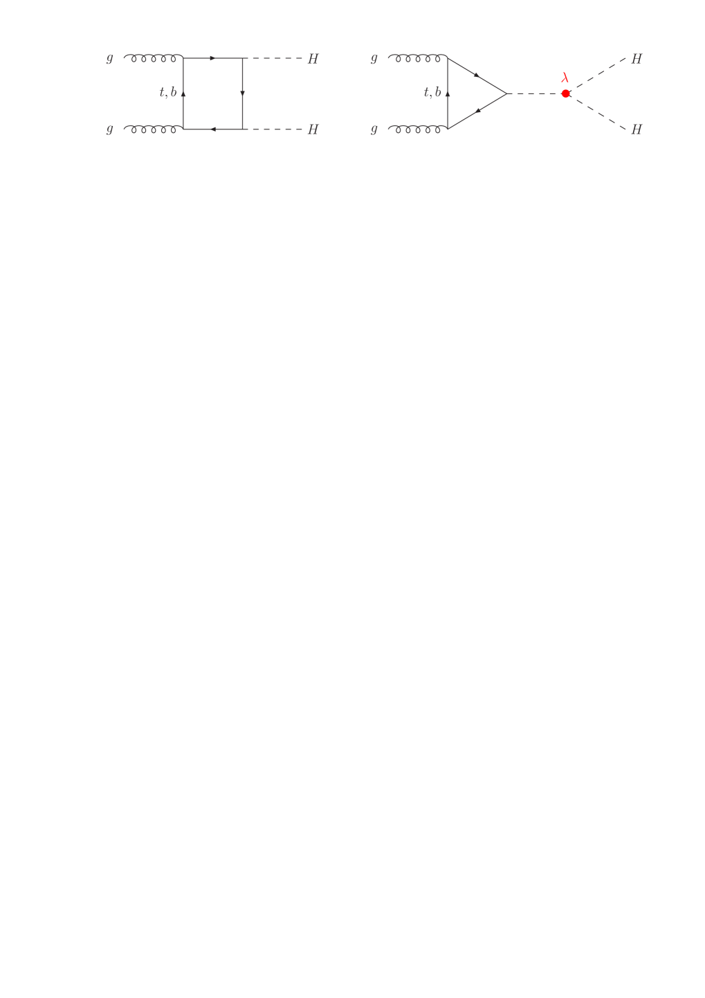
Figure 1: Generic diagrams contributing to Higgs-boson pair production via gluon fusion. The contribution of the trilinear Higgs coupling is marked in red.

The goal of this paper is to present in detail the calculation of Ref. Baglio:2018lrj of the full NLO corrections to Higgs pair production in gluon fusion. We rely on a direct numerical integration of the Feynman diagrams, without any tensor reduction. We extend the results presented in Ref. Baglio:2018lrj and study not only the LHC at center-of-mass energies of 13 and 14 TeV, but also present numbers for a potential high-energy upgrade of the LHC (HE-LHC) at 27 TeV Abada:2019ono and for a provisional 100 TeV proton collider within the Future-Circular-Collider (FCC) project  Abada:2019lih ; Benedikt:2018csr . Special emphasis will be given to the study of the theoretical uncertainties affecting the results and in particular the scale and scheme uncertainty related to the top-quark mass. We will also study the variation of the trilinear Higgs coupling and show that the NLO mass effects shift the minimum of the total cross section as a function of $\lambda_{H^{3}}$. They vary substantially over the range of $\lambda_{H^{3}}$ values.

The paper is organized as follows. We present the notation of our calculation in Section 2 and discuss the results at LO. In Section 3 we move to the NLO QCD corrections. We discuss the details of the calculation of the virtual corrections in Section 3.1. We describe the derivation of the real corrections in Section 3.2. Our numerical analysis is performed in Section 4. Finally, the conclusions are given in Section 5.

2 Leading-order cross section

At LO, Higgs-boson pair production via gluon fusion is mediated by the generic diagrams of Fig. 1, including all permutations of the external lines. There are triangle and box diagrams with the former involving the trilinear Higgs coupling through an $s$-channel Higgs exchange. The LO matrix element of $g(q_{1})g(q_{2})\to H(p_{1})H(p_{2})$ can be cast into the form

$${\cal M}(g^{a}g^{b}\to HH) = -i\,\frac{G_{F}\alpha_{s}(\mu_{R})Q^{2}}{2\sqrt{2}\pi}{\cal A}^{\mu\nu}\epsilon_{1\mu}\epsilon_{2\nu}\delta_{ab}$$

$$\mbox{with}\qquad{\cal A}^{\mu\nu} = F_{1}T_{1}^{\mu\nu}+F_{2}T_{2}^{\mu\nu}\,,$$

$$F_{1} = C_{\triangle}F_{\triangle}+F_{\Box}\,,\qquad\qquad\qquad F_{2}=G_{\Box}\,,$$

$$C_{\triangle} = \frac{\lambda_{H^{3}}v}{Q^{2}-M_{H}^{2}+iM_{H}\Gamma_{H}}$$

$$\mbox{and}\qquad Q^{2} = (p_{1}+p_{2})^{2}=m_{HH}^{2}$$ (4)

with $Q=m_{HH}$ denoting the invariant Higgs-pair mass. Here $a,b$ denote the color indices of the initial gluons, $\epsilon_{1/2}$ their polarization vectors, $\Gamma_{H}$ the total Higgs width, $G_{F}$ the Fermi constant and $\alpha_{s}(\mu_{R})$ the strong coupling at the renormalization scale $\mu_{R}$. Since in this work we neglect the small bottom-quark contribution, the LO function of the triangle-diagram contribution is given by the top-quark contribution,

$$F_{\triangle}(\tau_{t})=\tau_{t}\Big{[}1+(1-\tau_{t})f(\tau_{t})\Big{]}$$ (5)

with $\tau_{t}=4m_{t}^{2}/Q^{2}$ and the basic function

$$f(\tau) = \left\{\begin{array}[]{ll}\displaystyle\arcsin^{2}\frac{1}{\sqrt{\tau}}&\tau\geq 1\\ \displaystyle-\frac{1}{4}\left[\log\frac{1+\sqrt{1-\tau}}{1-\sqrt{1-\tau}}-i\pi\right]^{2}&\tau<1\end{array}\right.\,,$$ (8)

where $m_{t}$ denotes the top mass, while the more involved analytical expressions for $F_{\Box}$ and $G_{\Box}$ can be found in Ref. Plehn:1996wb . In the HTL, the LO form factors approach the values

$$F_{\triangle}\to\frac{2}{3},\qquad F_{\Box}\to-\frac{2}{3},\qquad G_{\Box}\to 0\,.$$ (9)

There are two tensor structures contributing which correspond to the total angular-momentum states with $S_{z}=0$ and $2$,

$$T_{1}^{\mu\nu} = g^{\mu\nu}-\frac{q_{1}^{\nu}q_{2}^{\mu}}{(q_{1}q_{2})}\,,$$

$$T_{2}^{\mu\nu} = g^{\mu\nu}+\frac{M_{H}^{2}q_{1}^{\nu}q_{2}^{\mu}}{p_{T}^{2}(q_{1}q_{2})}-2\frac{(q_{2}p_{1})q_{1}^{\nu}p_{1}^{\mu}}{p_{T}^{2}(q_{1}q_{2})}-2\frac{(q_{1}p_{1})p_{1}^{\nu}q_{2}^{\mu}}{p_{T}^{2}(q_{1}q_{2})}+2\frac{p_{1}^{\nu}p_{1}^{\mu}}{p_{T}^{2}}$$

$$\mbox{with}\quad p_{T}^{2} = 2\frac{(q_{1}p_{1})(q_{2}p_{1})}{(q_{1}q_{2})}-M_{H}^{2}\,,$$ (10)

where $p_{T}$ is the transverse momentum of each of the final-state Higgs bosons. Working in $n=4-2\epsilon$ dimensions, the following projectors on the two form factors can be constructed,

$$P_{1}^{\mu\nu}=\frac{(1-\epsilon)T_{1}^{\mu\nu}+\epsilon T_{2}^{\mu\nu}}{2(1-2\epsilon)}\,,\qquad\qquad P_{2}^{\mu\nu}=\frac{\epsilon T_{1}^{\mu\nu}+(1-\epsilon)T_{2}^{\mu\nu}}{2(1-2\epsilon)}\,,$$ (11)

such that

$$P_{1}^{\mu\nu}{\cal A}_{\mu\nu}=F_{1}\,,\qquad\qquad P_{2}^{\mu\nu}{\cal A}_{\mu\nu}=F_{2}\,.$$ (12)

Using these projectors, the explicit results of the two form factors $F_{1,2}$ can be obtained in a straightforward manner. The analytical expressions can be found in Refs. Glover:1987nx ; Plehn:1996wb . Working out the polarization and color sums of the matrix element of Eq. (4), the LO partonic cross section $\hat{\sigma}_{LO}$ is given by

$$\hat{\sigma}_{LO}=\frac{G_{F}^{2}\alpha_{s}^{2}(\mu_{R})}{512(2\pi)^{3}}\int_{\hat{t}_{-}}^{\hat{t}_{+}}d\hat{t}\Big{[}|F_{1}|^{2}+|F_{2}|^{2}\Big{]}$$ (13)

with the integration boundaries

$$\hat{t}_{\pm}=-\frac{1}{2}\left[Q^{2}-2M_{H}^{2}\mp Q^{2}\sqrt{1-4\frac{M_{H}^{2}}{Q^{2}}}\right]\,,$$ (14)

where the symmetry factor 1/2 for the identical Higgs bosons in the final state is taken into account. The LO hadronic cross section $\sigma_{LO}$ can then be derived by a convolution with the parton densities

$$\sigma_{LO}=\int_{\tau_{0}}^{1}d\tau\frac{d{\cal L}^{gg}}{d\tau}\hat{\sigma}_{LO}(Q^{2}=\tau s)$$ (15)

with the gluon luminosity, given in terms of the gluon densities $g(x,\mu_{F})$,

$$\frac{d{\cal L}^{gg}}{d\tau}=\int_{\tau}^{1}\frac{dx}{x}g(x,\mu_{F})g\left(\frac{\tau}{x},\mu_{F}\right)$$ (16)

at the factorization scale $\mu_{F}$ and the integration boundary $\tau_{0}=4M_{H}^{2}/s$, where $s$ denotes the hadronic center-of-mass (c.m.) energy squared. The differential cross section with respect to the invariant squared Higgs-pair mass $Q^{2}$ can be obtained as

$$\frac{d\sigma_{LO}}{dQ^{2}}=\left.\frac{d{\cal L}^{gg}}{d\tau}~{}\frac{\hat{\sigma}_{LO}(Q^{2})}{s}\right|_{\tau=\frac{Q^{2}}{s}}\,.$$ (17)

As can be expected from single Higgs-boson production via gluon fusion (see Graudenz:1992pv ; Spira:1995rr ; Harlander:2005rq ; Anastasiou:2009kn ; Aglietti:2006tp ), the NLO QCD corrections to these LO expressions will be large.

3 Next-to-leading-order corrections

The NLO QCD corrections to Higgs-pair production via gluon fusion have been computed in the HTL, a long time ago Dawson:1998py . The NLO result for the gluon-fusion cross section can be generically expressed as Dawson:1998py

$$\sigma_{NLO}(pp\rightarrow HH+X) = \sigma_{LO}+\Delta\sigma_{virt}+\Delta\sigma_{gg}+\Delta\sigma_{gq}+\Delta\sigma_{q\bar{q}}\,,$$

$$\sigma_{LO} = \int_{\tau_{0}}^{1}d\tau~{}\frac{d{\cal L}^{gg}}{d\tau}~{}\hat{\sigma}_{LO}(Q^{2}=\tau s)\,,$$

$$\Delta\sigma_{virt} = \frac{\alpha_{s}(\mu_{R})}{\pi}\int_{\tau_{0}}^{1}d\tau~{}\frac{d{\cal L}^{gg}}{d\tau}~{}\hat{\sigma}_{LO}(Q^{2}=\tau s)~{}C_{virt}(Q^{2})\,,$$

$$\Delta\sigma_{ij} = \frac{\alpha_{s}(\mu_{R})}{\pi}\int_{\tau_{0}}^{1}d\tau~{}\frac{d{\cal L}^{ij}}{d\tau}\int_{\tau_{0}/\tau}^{1}\frac{dz}{z}~{}\hat{\sigma}_{LO}(Q^{2}=z\tau s)\,C_{ij}(Q^{2},z)\qquad(ij=gg,gq,q\bar{q})\,,$$

$$C_{gg}(Q^{2},z) = -zP_{gg}(z)\log\frac{\mu_{F}^{2}}{\tau s}+6[1+z^{4}+(1-z)^{4}]\left(\frac{\log(1-z)}{1-z}\right)_{+}+d_{gg}(Q^{2},z)\,,$$

$$C_{gq}(Q^{2},z) = -\frac{z}{2}P_{gq}(z)\log\frac{\mu_{F}^{2}}{\tau s(1-z)^{2}}+d_{gq}(Q^{2},z)\,,$$

$$C_{q\bar{q}}(Q^{2},z) = d_{q\bar{q}}(Q^{2},z)$$ (18)

with $\hat{\sigma}_{LO}(Q^{2})$ denoting the partonic cross section at LO and the strong coupling $\alpha_{s}(\mu_{R})$ is evaluated at the renormalization scale $\mu_{R}$. The objects $d{\cal L}^{ij}/d\tau~{}(i,j=g,q,\bar{q})$ denote the parton-parton luminosities, defined analogously to $d{\cal L}^{gg}/d\tau$ of Eq. (16), using the quark densities $q(x,\mu_{F})$,

$$\frac{d{\cal L}^{gq}}{d\tau} = \sum_{q,\bar{q}}\int_{\tau}^{1}\frac{dx}{x}\Big{[}g(x,\mu_{F})q\left(\frac{\tau}{x},\mu_{F}\right)+q(x,\mu_{F})g\left(\frac{\tau}{x},\mu_{F}\right)\Big{]}\,,$$

$$\frac{d{\cal L}^{q\bar{q}}}{d\tau} = \sum_{q}\int_{\tau}^{1}\frac{dx}{x}\Big{[}q(x,\mu_{F})\bar{q}\left(\frac{\tau}{x},\mu_{F}\right)+\bar{q}(x,\mu_{F})q\left(\frac{\tau}{x},\mu_{F}\right)\Big{]}$$ (19)

at the factorization scale $\mu_{F}$ and $P_{ij}(z)~{}(i,j=g,q,\bar{q})$ are the specific Altarelli–Parisi splitting functions Altarelli:1977zs .

The quark-mass dependence is in general encoded in the LO cross section $\hat{\sigma}_{LO}(Q^{2})$ and the terms $C_{virt}(Q^{2})$, $d_{ij}(Q^{2},z)$ for the virtual and real corrections, respectively. These expressions can easily be converted into the differential cross section with respect to $Q^{2}$,

$$\frac{d\Delta\sigma_{virt}}{dQ^{2}} = \left.\frac{\alpha_{s}\left(\mu_{R}\right)}{\pi}~{}\frac{d{\cal L}^{gg}}{d\tau}~{}\frac{\hat{\sigma}_{LO}\left(Q^{2}\right)}{s}~{}C_{virt}\left(Q^{2}\right)\right|_{\tau=\frac{Q^{2}}{s}},$$

$$\frac{d\Delta\sigma_{ij}}{dQ^{2}} = \left.\frac{\alpha_{s}\left(\mu_{R}\right)}{\pi}\int_{\frac{Q^{2}}{s}}^{1}\frac{dz}{z^{2}}~{}\frac{d{\cal L}^{ij}}{d\tau}~{}\frac{\hat{\sigma}_{LO}\left(Q^{2}\right)}{s}~{}C_{ij}(Q^{2},z)\right|_{\tau=\frac{Q^{2}}{zs}}\,,$$ (20)

while the differential cross section at LO is given in Eq. (17).

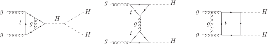
Figure 2: Typical two-loop triangle (left), one-particle reducible (middle) and box (right) diagrams contributing to Higgs-pair production via gluon fusion at NLO.

Within the HTL, the Higgs coupling to gluons can be described by an effective Lagrangian Ellis:1975ap ; Shifman:1979eb ; Inami:1982xt ; Spira:1995rr ; Kniehl:1995tn

$${\cal L}_{\mathrm{eff}}=\frac{\alpha_{s}}{12\pi}G^{a\mu\nu}G^{a}_{\mu\nu}\left(C_{1}\frac{H}{v}-C_{2}\frac{H^{2}}{2v^{2}}\right)$$ (21)

involving the Wilson coefficients ($L_{t}=\log\mu_{R}^{2}/m_{t}^{2}$) Chetyrkin:1997iv ; Kramer:1996iq ; Dawson:1998py ; Schroder:2005hy ; Baikov:2016tgj ; Grigo:2014jma ; Spira:2016zna ; Gerlach:2018hen

$$C_{1} = 1+\frac{11}{4}\frac{\alpha_{s}}{\pi}+\left\{\frac{2777}{288}+\frac{19}{16}L_{t}+N_{F}\left(\frac{L_{t}}{3}-\frac{67}{96}\right)\right\}\left(\frac{\alpha_{s}}{\pi}\right)^{2}+{\cal O}(\alpha_{s}^{3})\,,$$

$$C_{2} = C_{1}+\left(\frac{35}{24}+\frac{2}{3}N_{F}\right)\left(\frac{\alpha_{s}}{\pi}\right)^{2}+{\cal O}(\alpha_{s}^{3})$$ (22)

that are known up to N⁴LO Schroder:2005hy ; Baikov:2016tgj ; Spira:2016zna . Since the top quark is integrated out, the number of active flavours has been chosen as $N_{F}=5$. If these effective Higgs couplings to gluons in the calculation of the NLO QCD corrections are used, the calculation of these is simplified to a one-loop calculation for the virtual corrections and a tree-level one for the matrix elements of the real corrections. The terms $C_{virt}(Q^{2})$ and $d_{ij}(Q^{2},z)$, for the virtual and real corrections, approach in the HTL the simple expressions

$$C_{virt}(Q^{2}) \to \frac{11}{2}+\pi^{2}+C^{\infty}_{\triangle\triangle}+\frac{33-2N_{F}}{6}\log\frac{\mu_{R}^{2}}{Q^{2}},$$

$$C_{\triangle\triangle} = \Re e~{}\frac{\int_{\hat{t}_{-}}^{\hat{t}_{+}}d\hat{t}\left\{c_{1}\left[(C_{\triangle}F_{\triangle}+F_{\Box})+\frac{p_{T}^{2}}{\hat{t}}G_{\Box}\right]^{*}+(\hat{t}\leftrightarrow\hat{u})\right\}}{\int_{\hat{t}_{-}}^{\hat{t}_{+}}d\hat{t}\left\{|C_{\triangle}F_{\triangle}+F_{\Box}|^{2}+|G_{\Box}|^{2}\right\}},$$

$$C^{\infty}_{\triangle\triangle} = \left.C_{\triangle\triangle}\right|_{c_{1}=2/9},$$

$$d_{gg}(Q^{2},z)\!\!\! \to \!\!\!-\frac{11}{2}(1-z)^{3}\,,\ d_{gq}(Q^{2},z)\to\frac{2}{3}z^{2}-(1-z)^{2}\,,\ d_{q\bar{q}}(Q^{2},z)\to\frac{32}{27}(1-z)^{3}\,,$$ (23)

where $\hat{s},\hat{t},\hat{u}$ ($\hat{s}=Q^{2}$ at LO and for the virtual corrections) denote the partonic Mandelstam variables and $C_{\triangle\triangle}$ is the contribution of the one-particle reducible diagrams, see Fig. 2.

At NLO QCD, the full mass dependence of the LO partonic cross section has been taken into account, while keeping the virtual corrections $C_{virt}$ and the real corrections $d_{ij}$ in the HTL (“Born-improved” approach) Dawson:1998py . This yields a reasonable approximation for smaller invariant Higgs-pair masses and approximates the full NLO result of the total cross section within about 15% Borowka:2016ehy ; Borowka:2016ypz ; Baglio:2018lrj . The NLO QCD corrections in the HTL increase the cross section by $80-90\%$ Dawson:1998py . Within the Born-improved HTL, the NNLO QCD corrections have been obtained in Refs. deFlorian:2013uza ; deFlorian:2013jea ; Grigo:2014jma increasing the total cross section by a moderate amount of $20-30\%$ deFlorian:2013jea . Beyond these NNLO QCD corrections, the soft-gluon resummation (threshold resummation) has been performed at next-to-next-to-leading logarithmic (NNLL) accuracy for the total cross section and invariant mass distribution, modifying the total cross section further by a small amount if the central scales are chosen as $\mu_{R}=\mu_{F}=Q/2$ Shao:2013bz ; deFlorian:2015moa . Very recently, the N³LO QCD corrections have been computed in the Born-improved HTL resulting in a small modification of the cross section beyond NNLOBanerjee:2018lfq ; Chen:2019lzz ; Chen:2019fhs ; Spira:2016zna . These N³LO QCD corrections in the HTL have been merged with the full top-mass effects of the NLO calculation Chen:2019fhs .

The calculations in the HTL have been improved by several steps including mass effects partially at NLO. The full mass effects in the real correction terms $d_{ij}$ have been included by means of the full one-loop real matrix elements for $gg\to HHg,gq\to HHq,q\bar{q}\to HHg$. This improvement reduces the Born-improved HTL prediction for the total cross section by about 10% Frederix:2014hta ; Maltoni:2014eza and is called the “FTapprox” approximation. The calculation of the full real matrix elements has been performed by using the MG5_aMC@NLO framework Alwall:2014hca ; Hirschi:2015iia . Another improvement has been achieved by an asymptotic large-top-mass expansion of the full NLO corrections at the level of the integral Grigo:2013rya and the integrand Grigo:2015dia . This indicated sizable mass effects in the virtual two-loop corrections alone. In addition, the large top-mass expansion has been extended to the virtual NNLO QCD corrections resulting in 5% mass effects estimated on top of the NLO result Grigo:2015dia . The large-top-mass expansion of the NLO QCD corrections has been used to perform a conformal mapping of the expansion parameter and to apply Padé approximants. In this way, an approximation of the full calculation has been achieved for $Q$ values up to about 700 GeV Grober:2017uho . Another approximation builds on an expansion in terms of a variable that dominantly corresponds to the transverse momentum of the Higgs bosons. The results of this approach show good agreement with the full calculation for $Q$ values up to about 900 GeV Bonciani:2018omm . Analytical results are also available in the large-$Q$ limit Davies:2018qvx . The latter have recently been combined with the numerical results of Refs. Borowka:2016ehy ; Borowka:2016ypz for the full QCD corrections Davies:2019dfy . In the following, we will discuss the details of our NLO calculation.

3.1 Virtual corrections

Typical diagrams of the two-loop virtual corrections are shown in Fig. 2. They can be arranged in three different classes: (a) triangle, (b) one-particle-reducible and (c) box diagrams. They contribute to the coefficient $C_{virt}(Q^{2})$ of Eq. (18),

$$C_{virt}(Q^{2})=2\Re e~{}\frac{\int_{\hat{t}_{-}}^{\hat{t}_{+}}d\hat{t}\left\{(C_{\triangle}F_{\triangle}+F_{\Box})^{*}[C_{\triangle}(\Delta F_{\triangle})+\Delta F_{\Box}]+G_{\Box}^{*}(\Delta G_{\Box})\right\}}{\int_{\hat{t}_{-}}^{\hat{t}_{+}}d\hat{t}\left\{|C_{\triangle}F_{\triangle}+F_{\Box}|^{2}+|G_{\Box}|^{2}\right\}},$$ (24)

where $\Delta F_{\triangle},\Delta F_{\Box}$ and $\Delta G_{\Box}$ denote the virtual corrections to the corresponding LO form factors. While $\Delta F_{\triangle}$ involves only virtual corrections to the triangle diagram, $\Delta F_{\Box}$ and $\Delta G_{\Box}$ acquire contributions from the one-particle-reducible and box diagrams.

3.1.1 Triangle diagrams

Figure 3: Two-loop triangle diagrams contributing to Higgs-pair production via gluon fusion.

The generic 2-loop triangle diagrams contributing to the virtual coefficient $C_{virt}(Q^{2})$ are shown in Fig. 3. They only contribute to the spin-0 form factor $F_{1}$ of Eq. (4) and can be parametrized as the correction $\Delta F_{\triangle}$ to the form factor $F_{\triangle}$,

$$\Delta F_{\triangle}=\frac{\alpha_{s}}{\pi}~{}{\cal C}_{virt}(Q^{2})~{}F_{\triangle}\,,$$ (25)

where ${\cal C}_{virt}(Q^{2})$ denotes the complex virtual coefficient relative to the LO form factor $F_{\triangle}$ of the amplitude. This virtual coefficient is related to the single-Higgs case so that the relative QCD corrections can be simply obtained from the known (complex) virtual coefficient ${\cal C}^{H}_{virt}(M_{H}^{2})$ of single Higgs production Spira:1995rr ; Graudenz:1992pv ; Harlander:2005rq ; Anastasiou:2009kn ; Aglietti:2006tp ,

$${\cal C}_{virt}(Q^{2})=\left.{\cal C}^{H}_{virt}(M_{H}^{2})\right|_{M_{H}^{2}\to Q^{2}}\,.$$ (26)

In the HTL, this virtual coefficient (before renormalization) approaches the expression

$${\cal C}_{virt}(Q^{2})\to\frac{\Gamma(1-\epsilon)}{\Gamma(1-2\epsilon)}\left(\frac{4\pi\mu_{0}^{2}(1-i\bar{\epsilon})}{-Q^{2}}\right)^{\epsilon}\left\{-\frac{3}{2\epsilon^{2}}+\frac{3}{4}-\frac{\pi^{2}}{4}\right\}$$ (27)

with the ’t Hooft scale $\mu_{0}$, where the (infinitesimal) regulator $\bar{\epsilon}$ defines the proper analytical continuation of this expression. This result has to be followed by the renormalization of the strong coupling $\alpha_{s}$ and the top mass $m_{t}$ that will be discussed in Section 3.1.4. In addition, we have subtracted the HTL to obtain the pure top-mass effects at NLO (relative to the massive LO expression $F_{\triangle}$) to ensure that in the end the results of the program Hpair hpair can be added back. This last step will be discussed in Section 3.1.4, too.

3.1.2 One-particle-reducible diagrams

The one-particle-reducible contribution is depicted in Fig. 2 (middle diagram), where a second diagram with the initial gluons interchanged has to be added. These will constitute the $\hat{t}$- and $\hat{u}$-channel parts where the second is related to the first just by the interchange $\hat{t}\leftrightarrow\hat{u}$ [see $C_{\triangle\triangle}$ of Eq. (23)]. The analytical expression of the coefficient $c_{1}$ can be related to the top contribution of the process $H\to Z\gamma$ Cahn:1978nz ; Bergstrom:1985hp . The basic building block will be the one-loop contribution of the Higgs coupling to an on-shell and an off-shell gluon that is described, after translating all couplings and masses, by the “effective” Feynman rule,

where the functions $I_{1,2}$ are defined as Gunion:1989we

$$I_{1}(\tau,\lambda) = \frac{\tau\lambda}{2(\tau-\lambda)}+\frac{\tau^{2}\lambda^{2}}{2(\tau-\lambda)^{2}}\left[f(\tau)-f(\lambda)\right]+\frac{\tau^{2}\lambda}{(\tau-\lambda)^{2}}\left[g(\tau)-g(\lambda)\right],$$

$$I_{2}(\tau,\lambda) = -\frac{\tau\lambda}{2(\tau-\lambda)}\left[f(\tau)-f(\lambda)\right],$$ (28)

with $\tau=4m_{t}^{2}/m_{H}^{2}$, $\lambda=4m_{t}^{2}/q_{2}^{2}$ and the basic functions

$$g(\tau) = \left\{\begin{array}[]{ll}\displaystyle\sqrt{\tau-1}\arcsin\frac{1}{\sqrt{\tau}}&\tau\geq 1\\ \displaystyle\frac{\sqrt{1-\tau}}{2}\left[\log\frac{1+\sqrt{1-\tau}}{1-\sqrt{1-\tau}}-i\pi\right]&\tau<1\end{array}\right.$$ (31)

and $f(\tau)$ defined in Eq. (8). Implementing this building block for the two top loops of the one-particle-reducible diagrams, one arrives at the final coefficient $c_{1}$ of Eq. (23),

$$c_{1} = 2\Big{[}I_{1}(\tau,\lambda_{\hat{t}})-I_{2}(\tau,\lambda_{\hat{t}})\Big{]}^{2}$$ (32)

with $\lambda_{\hat{t}}=4m_{t}^{2}/\hat{t}$ (and $\lambda_{\hat{u}}=4m_{t}^{2}/\hat{u}$ for the $\hat{t}\leftrightarrow\hat{u}$ interchanged contribution accordingly). This expression, inserted in the coefficient $C_{\triangle\triangle}$ of Eq. (23), determines the contribution of the one-particle-reducible diagrams analytically and agrees with the previous calculation of Ref. Degrassi:2016vss . In the HTL, this coefficient approaches the value $c_{1}\to 2/9$ in accordance with Eq. (23). We have subtracted the HTL with $c_{1}=2/9$ from the coefficient $C_{\triangle\triangle}$ in order to account for the NLO top-mass effects only so that eventually the results of the program Hpair hpair can be added back. While the total effect of the one-particle-reducible contributions on the total cross section ranges below the per-cent level, the finite mass effects at NLO contribute less than one per mille.

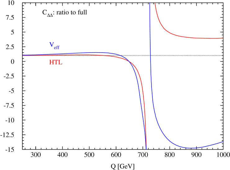
Figure 4: Comparison of the approximation of Ref. deFlorian:2017qfk (blue) for the one-particle-reducible contributions and the HTL (red), both normalized to the full analytical expression. The singularity at about 720 GeV is due to a sign change of the exact expression.

Reference deFlorian:2017qfk has proposed an approximation of this one-particle-reducible contribution in terms of the triangle form factor of two on-shell external gluons,

$$C_{\triangle\triangle} = \Re e~{}\frac{\int_{\hat{t}_{-}}^{\hat{t}_{+}}d\hat{t}\left[(C_{\triangle}F_{\triangle}+F_{\Box})^{*}V_{eff}^{2}\right]}{\int_{\hat{t}_{-}}^{\hat{t}_{+}}d\hat{t}\left\{|C_{\triangle}F_{\triangle}+F_{\Box}|^{2}+|G_{\Box}|^{2}\right\}},$$

$$V_{eff} = F_{\triangle}(\bar{\tau}_{t})$$ (33)

with $\bar{\tau}_{t}=16m_{t}^{2}/Q^{2}$ [i.e. $\tau_{t}$ of Eq. (5) evaluated at half the invariant Higgs-pair mass $Q/2$ instead of $Q$], where the function $F_{\triangle}$ can be found in Eq. (5). Since Ref. deFlorian:2017qfk works in the HTL, the contribution of the second form factor $F_{2}$ vanishes, i.e. $G_{\Box}\to 0$, and the approximation $V_{eff}^{2}/2$ is in fact treated as an approximation for the coefficient $c_{1}$ of the exact expression of $C_{\triangle\triangle}$ as given in Eq. (23). Thus, the approximate expression involving the coefficient $c_{1}$ has to be compared to the corresponding expression involving the exact coefficient $c_{1}$ of Eq. (32). This comparison is presented, normalized to the exact expression, in Fig. 4 and shows that the approximation of Ref. deFlorian:2017qfk is not better than the HTL.

3.1.3 Box diagrams

The third class of two-loop contributions to the virtual corrections is given by the box diagrams. The generic box diagrams are shown in Figs. 19–21 in the Appendix. The simultaneous exchange of the gluons and Higgs bosons has to be added to complete the set of diagrams. The only exception is diagram 44 that is already totally symmetric so that in the final end there are 93 two-loop box diagrams. The generic 47 diagrams are grouped into 6 topology classes. The first 5 topologies contain only a virtual threshold for $Q^{2}>4m_{t}^{2}$. The diagrams of topology 6 on the other hand develop a second threshold for $Q^{2}>0$, because two virtual gluon lines next to the external gluons can be cut. This implies that the form factors are complex in the entire $Q^{2}$ range. Therefore, a dedicated treatment of this last topology in terms of a suitably constructed infrared subtraction term to isolate the associated infrared singularities is required.

In the following, we will exemplify our method for the boxes 39 of topology 5 and 45 of topology 6. The diagrams of topologies 1–5 are treated analogously to box 39 and those of topology 6 analogously to box 45. The algebraic manipulation of the traces and projections onto the form factors have been performed with the help of the symbolic tools FORM Vermaseren:2000nd ; Kuipers:2012rf , Reduce Hearn:1971zza , and Mathematica Mathematica . Our method of Feynman parametrization and end-point subtraction to isolate the ultraviolet singularities for the numerical integration has first been applied to the NLO two-loop QCD corrections to $H\to\gamma\gamma,Z\gamma$ in Refs. Djouadi:1990aj ; Spira:1991tj and later to the squark-loop contributions to $h,H\leftrightarrow gg,\gamma\gamma$ within the minimal supersymmetric extension of the SM Muhlleitner:2006wx . The method of the infrared subtraction as applied to topology 6 originates from numerical cross checks of the full NLO QCD corrections to single Higgs production in Refs. Spira:1995es ; Spira:1995rr ; Graudenz:1992pv ; Muhlleitner:2006wx . The stabilization of virtual thresholds by integration by parts of the integrand has first been applied to the SUSY–QCD corrections to single Higgs production in Refs. Muhlleitner:2010nm ; Muhlleitner:2010zz . The basic idea behind the integration by parts is to reduce the power of the threshold-singular denominator and in this way to stabilize the numerical integration. The treatment of the thresholds in our approach is performed by replacing the squared top mass $m_{t}^{2}$ by a complex counter part

$$m_{t}^{2}\to m_{t}^{2}(1-i\bar{\epsilon})$$ (34)

with a positive regulator $\bar{\epsilon}>0$ to ensure proper micro-causality. This defines the analytical continuation of our two-loop box integrals. In the following, the parameter $\bar{\epsilon}$ will be kept finite in our numerical analysis, while the narrow-width limit $\bar{\epsilon}\to 0$ is achieved by a Richardson extrapolation Richardson . This will be discussed in more detail in the following paragraphs.

Box 39

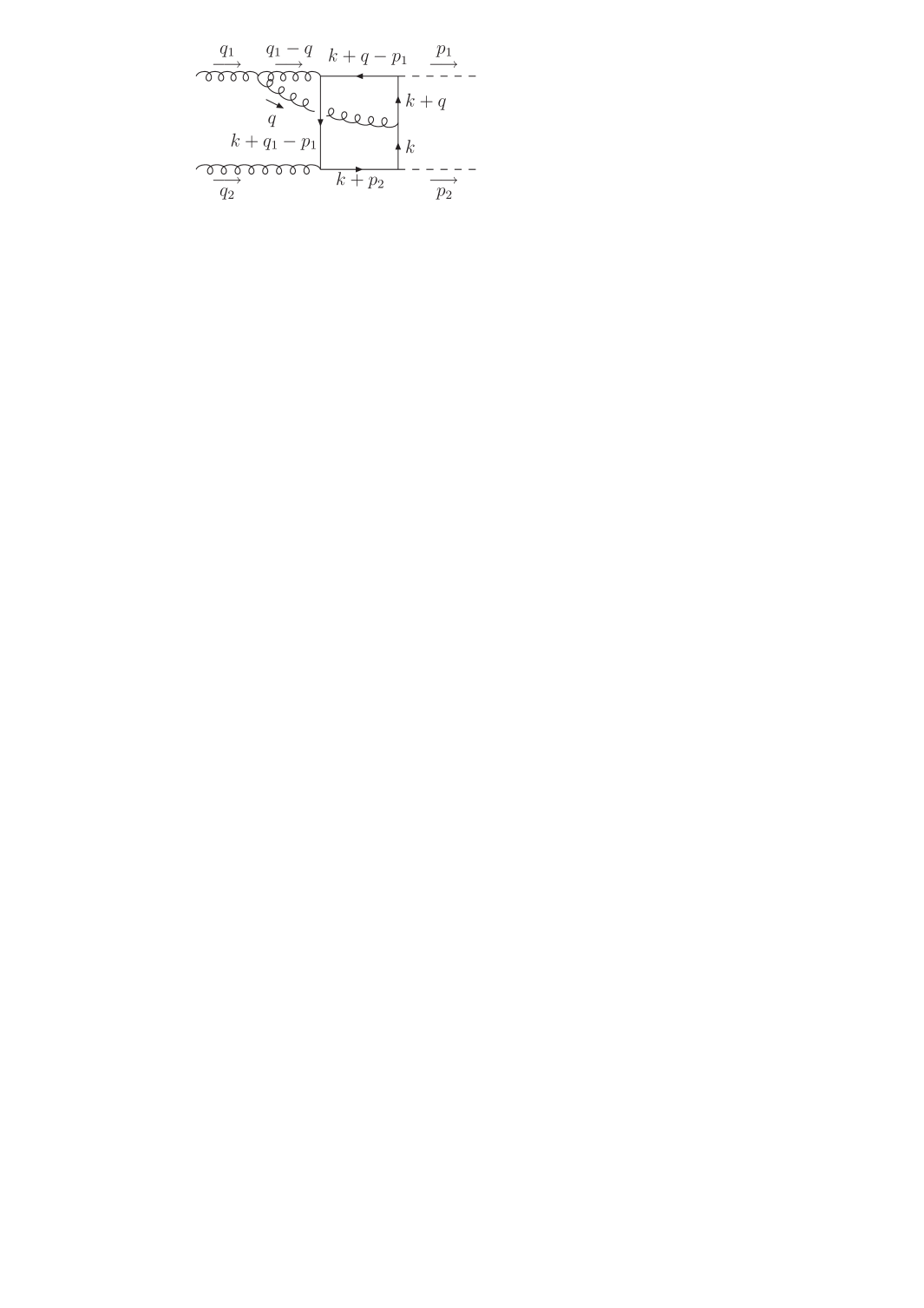
Figure 5: Explicit definitions of the virtual momenta in box 39.

Using the definition of real and virtual momenta as in Fig. 5, the contribution to the tensor $A^{\mu\nu}$ [see Eq. (4)] of the virtual two-loop corrections is given by

$$A_{39}^{\mu\nu} = \frac{3}{16}\,\frac{\alpha_{s}}{\pi}\,(4\pi)^{4}\,B_{39}^{\mu\nu}\,,$$

$$B_{39}^{\mu\nu}\!\! \!\!\!\!=\!\!\!\! \!\!\int\frac{d^{n}kd^{n}q}{(2\pi)^{2n}}\frac{Tr\Big{\{}(\,\!\!\not\!{k}+\!\!\not\!{q}-\!\!\not\!{p}_{1}+m_{t})(\,\!\!\not\!{k}+\!\!\not\!{q}+m_{t})\gamma^{\sigma}(\,\!\!\not\!{k}+m_{t})(\!\!\not\!{k}+\!\!\not\!{p}_{2}+m_{t})\gamma^{\nu}(\,\!\!\not\!{k}+\!\!\not\!{q}_{1}-\!\!\not\!{p}_{1}+m_{t})\gamma^{\rho}\Big{\}}}{[(k+q)^{2}-m_{t}^{2}][(k+q-p_{1})^{2}-m_{t}^{2}][(k+p_{2})^{2}-m_{t}^{2}][(k+q_{1}-p_{1})^{2}-m_{t}^{2}]}$$ (35)

$$\qquad\times~{}\frac{g_{\rho\sigma}(2q-q_{1})^{\mu}-g^{\mu}_{\rho}(q-2q_{1})_{\sigma}-g^{\mu}_{\sigma}(q+q_{1})_{\rho}}{(k^{2}-m_{t}^{2})(q-q_{1})^{2}q^{2}}\,,$$

where $k,q$ are the loop momenta that are integrated over. The Feynman parametrization is first performed for the integration over $k$. We provide Feynman parameters $x_{1},\ldots,x_{4}$ for the first four propagators in the denominator and $1-\sum_{i}x_{i}$ for the last one ($k^{2}-m_{t}^{2}$). Performing the substitutions

$$x_{1}=(1-x)(1-y)\,,\quad x_{2}=(1-x)y\,,\quad x_{3}=xzr\,,\quad x_{4}=xz(1-r)\,,$$ (36)

we arrive at a four-dimensional integral over $x,y,z,r$ with integration boundaries from 0 to 1. To symmetrize the $n$-dimensional $k$-integration, we have to perform the shift

$$k \to k-Q_{1}\,,$$

$$Q_{1} = (1-x)q+xzq_{1}+xzrq_{2}-[(1-x)y+xz]p_{1}\,,$$ (37)

in both the numerator and denominator. The residual (properly normalized) denominator after the $k$-integration is treated as a propagator for the second loop integration over $q$. We attribute additional Feynman parameters $x_{5},x_{6}$ to this residual propagator and the next one [$(q-q_{1})^{2}$] and $1-x_{5}-x_{6}$ for the last one ($q^{2}$) in Eq. (35). Performing the substitution

$$x_{5}=s\,,\quad x_{6}=(1-s)t\,,$$ (38)

we again arrive at integrals over $s,t$ from 0 to 1. This latter parametrization requires the shift

$$q \to q-Q_{2}\,,$$

$$Q_{2} = -[zs+(1-s)t]q_{1}-zrsq_{2}-(y-z)sp_{1}$$ (39)

in the numerator and denominator to be able to perform the loop integration over $q$ symmetrically. After projecting on the two form factors, we finally arrive at integrals of the type

$$\Delta F_{i}=\frac{\alpha_{s}}{\pi}~{}\Gamma(1+2\epsilon)\left(\frac{4\pi\mu_{0}^{2}}{m_{t}^{2}}\right)^{2\epsilon}\int_{0}^{1}d^{6}x~{}\frac{x^{\epsilon}(1-x)^{\epsilon}s^{-1-\epsilon}H_{i}(\vec{x})}{N^{3+2\epsilon}(\vec{x})}$$ (40)

with $\vec{x}=(x,y,z,r,s,t)$ and $d^{6}x=dx\,dy\,dz\,dr\,ds\,dt$. $H_{i}(\vec{x})$ denotes the full numerator, including regular factors of the Jacobians due to the Feynman parametrization and substitutions, and singular as well as higher powers of the dimensional regulator $\epsilon$, and $N(\vec{x})$ the final denominator,

$$N(\vec{x}) = 1+\rho_{s}xzr\Big{\{}xz+(1-x)[zs+(1-s)t]\Big{\}}$$ (41)

$$\quad-\rho_{t}x\Big{\{}z(1-y-r)+(y-z)[z+(1-x)(1-s)(t-z)]\Big{\}}$$

$$\quad+\rho_{u}xzr\Big{\{}xz+(1-x)[zs+(1-s)y]\Big{\}}$$

$$\quad-\rho_{H}\Big{\{}[xz+(1-x)y][1-xz-(1-x)y]-x(1-x)s(y-z)^{2}\Big{\}}\,,$$

where we define $\rho_{s}=\hat{s}/m_{t}^{2}=Q^{2}/m_{t}^{2}$, $\rho_{t}=(\hat{t}-M_{H}^{2})/m_{t}^{2}$, $\rho_{u}=(\hat{u}-M_{H}^{2})/m_{t}^{2}$ and $\rho_{H}=M_{H}^{2}/m_{t}^{2}$. The singular powers in $\epsilon$ of $H_{i}(\vec{x})$ arise from powers of $k^{2}$ and $q^{2}$ in the numerators of the final integrations of the loop momenta $k$ and $q$. It is important that the final denominator develops the form of $1+O(1/m_{t}^{2})$ to ensure that no further ultraviolet nor infrared singularities arise from this part of the integrand.

The integral for $\Delta F_{i}$ of Eq. (40) is singular for $s\to 0$. To separate this singularity from the integral, we perform an endpoint subtraction,

$$\Delta F_{i} = \frac{\alpha_{s}}{\pi}~{}\Gamma(1+\epsilon)\frac{\Gamma(1-\epsilon)}{\Gamma(1-2\epsilon)}\left(\frac{4\pi\mu_{0}^{2}}{m_{t}^{2}}\right)^{2\epsilon}\left[\Delta F_{i,1}+\Delta F_{i,2}\right]\,,$$

$$\Delta F_{i,1} = \int_{0}^{1}\frac{d^{6}x}{s}\left\{\frac{H_{i}(\vec{x})}{N^{3}(\vec{x})}(1+\epsilon L)-\left.\frac{H_{i}(\vec{x})}{N^{3}(\vec{x})}\right|_{s=0}(1+\epsilon L_{0})\right\}\,,$$

$$\Delta F_{i,2} = -\frac{1}{\epsilon}\int_{0}^{1}d^{5}x\left.\frac{H_{i}(\vec{x})}{N^{3}(\vec{x})}\right|_{s=0}\left[1+\epsilon L_{1}+\epsilon^{2}\left(\frac{L_{1}^{2}}{2}+3\zeta_{2}\right)\right]$$

$$\mbox{with}\qquad L = \log\frac{x(1-x)}{s}-2\log N(\vec{x})\,,$$

$$L_{0} = \log\frac{x(1-x)}{s}-2\log N(\vec{x})|_{s=0}\,,$$

$$L_{1} = \log[x(1-x)]-2\log N(\vec{x})|_{s=0}\,,$$ (42)

where in the second term $\Delta F_{i,2}$ the integration over $s$ has been performed analytically and the integration measure is given by $d^{5}x=dx\,dy\,dz\,dr\,dt$. It should be noted that in the terms $L,L_{0},L_{1}$ the logarithms of the denominator $N$ need to be linear in $N$ to be consistent with the analytical continuation along the proper Riemann sheet. We have checked numerically that the first (subtracted) part $\Delta F_{i,1}$ is finite for each order in the dimensional regulator $\epsilon$ by introducing cuts in the integration boundaries, i.e. integrating from $\tilde{\epsilon}$ to $1-\tilde{\epsilon}$, varying $\tilde{\epsilon}$ down to $10^{-10}$ and checking that the integrals become independent of $\tilde{\epsilon}$.

These integrals are numerically stable below the virtual $t\bar{t}$-threshold, i.e. for $Q^{2}<4m_{t}^{2}$ or $\rho_{s}<4$. However, above this threshold, the integrals have to be stabilized. We have achieved this stabilization by means of integration by parts with respect to the Feynman parameter $z$. The denominator is a quadratic polynomial in $z$,

$$N(\vec{x}) = az^{2}+bz+c$$

$$\mbox{with}\qquad a = x[\rho_{s}r+\rho_{t}+\rho_{u}r+\rho_{H}][1-(1-x)(1-s)]\,,$$

$$b = \rho_{s}x(1-x)r(1-s)t-\rho_{t}x[1-r-(1-x)(1-s)(y+t)]$$

$$+ \rho_{u}x(1-x)yr(1-s)-\rho_{H}x[1-2(1-x)y(1-s)]\,,$$

$$c = 1-\rho_{t}x(1-x)y(1-s)t-\rho_{H}(1-x)y[1-y+xy(1-s)]\,.$$ (43)

To simplify the integration by parts, we insert a unit factor $\Delta/\Delta$ with $\Delta=4ac-b^{2}$ in the integrand and replace $\Delta$ in the numerator by the expression

$$\Delta=4aN-(\partial_{z}N)^{2}=4aN-(2az+b)^{2}\,.$$ (44)

Then the following manipulation can be performed,

$$\int_{0}^{1}dz~{}\frac{H_{i}(\vec{x})}{N^{3}} = \frac{1}{\Delta}\left\{\left.\left[\frac{2a+b}{2N^{2}}H_{i}(\vec{x})+\frac{\partial_{z}H_{i}(\vec{x})}{2N}\right]\right|_{z=1}-\left.\left[\frac{b}{2N^{2}}H_{i}(\vec{x})+\frac{\partial_{z}H_{i}(\vec{x})}{2N}\right]\right|_{z=0}\right.$$ (45)

$$\left.+\int_{0}^{1}dz~{}\left[\frac{3a}{N^{2}}H_{i}(\vec{x})-\frac{\partial_{z}^{2}H_{i}(\vec{x})}{2N}\right]\right\}$$

and analogously for integrals involving additional powers of $\log N$ factors in the numerator of the integrand. The progress achieved with these integrations by parts is that the maximal power of the denominator in the new integral is reduced by one compared to the original integral. One could perform additional integrations by parts with respect to another Feynman parameter. However, we did not investigate this further, since the stability we achieved at this point has been sufficient for the numerical integrations for the top loops.

After performing the integrations by parts, the integral is stable for regulators $\bar{\epsilon}$ [see Eq. (34)] down to $0.05$ for the relevant Higgs mass, top mass and $Q^{2}$ range. Since this is still apart from the plateau of the narrow-width limit, we performed a Richardson extrapolation Richardson from finite values of $\bar{\epsilon}$ down to zero. Richardson extrapolation is possible since the $\bar{\epsilon}$-dependence of the integral is polynomial for small values of $\bar{\epsilon}$. The basic principle behind this extrapolation method is very simple: let a function $f(\bar{\epsilon})$ behave for small $\bar{\epsilon}$ as

$$f(\bar{\epsilon})=f(0)+{\cal O}(\bar{\epsilon}^{n})\,.$$ (46)

If we know $f(\bar{\epsilon})$ for two different values $\bar{\epsilon}$ and $t\bar{\epsilon}$, we can construct the new function

$$R_{1}(\bar{\epsilon},t)=\frac{t^{n}f(\bar{\epsilon})-f(t\bar{\epsilon})}{t^{n}-1}\,.$$ (47)

This function shows a better convergence towards the value at $\bar{\epsilon}=0$,

$$R_{1}(\bar{\epsilon},t)=f(0)+{\cal O}(\bar{\epsilon}^{n+1})\,.$$ (48)

Our integrals $I(\bar{\epsilon})$ behave for small values of $\bar{\epsilon}$ as

$$I(\bar{\epsilon})=I(0)+{\cal O}(\bar{\epsilon})$$ (49)

so that the first new extrapolation function in our case is given by

$$R_{1}(\bar{\epsilon},t)=\frac{tI(\bar{\epsilon})-I(t\bar{\epsilon})}{t-1}=I(0)+{\cal O}(\bar{\epsilon}^{2})\,.$$ (50)

Using an additional value of $\bar{\epsilon}$, this method can be repeated iteratively for the new function obtained by applying Eq. (47),

$$R_{2}(\bar{\epsilon},t)=\frac{t^{2}R_{1}(\bar{\epsilon})-R_{1}(t\bar{\epsilon})}{t^{2}-1}=I(0)+{\cal O}(\bar{\epsilon}^{3})\,.$$ (51)

In this way, the estimated error is reduced by each additional iteration. We have used this method for a set of $\bar{\epsilon}$ separated by factors of $t=2$. Then, we obtain the following extrapolation polynomials,

$$R_{1}(\bar{\epsilon}) = 2I(\bar{\epsilon})-I(2\bar{\epsilon})=I(0)+{\cal O}(\bar{\epsilon}^{2})\,,$$

$$R_{2}(\bar{\epsilon}) = \frac{1}{3}\Big{[}8I(\bar{\epsilon})-6I(2\bar{\epsilon})+I(4\bar{\epsilon})\Big{]}=I(0)+{\cal O}(\bar{\epsilon}^{3})\,,$$

$$R_{3}(\bar{\epsilon}) = \frac{1}{21}\Big{[}64I(\bar{\epsilon})-56I(2\bar{\epsilon})+14I(4\bar{\epsilon})-I(8\bar{\epsilon})\Big{]}=I(0)+{\cal O}(\bar{\epsilon}^{4})\,,$$

$$R_{4}(\bar{\epsilon}) = \frac{1}{315}\Big{[}1024I(\bar{\epsilon})-960I(2\bar{\epsilon})+280I(4\bar{\epsilon})-30I(8\bar{\epsilon})+I(16\bar{\epsilon})\Big{]}=I(0)+{\cal O}(\bar{\epsilon}^{5})$$ (52)

and so on. We have used extrapolation polynomials up to $R_{9}(\bar{\epsilon})$. To determine the extrapolation error, we have chosen different sets of $\bar{\epsilon}$ values and derived the spread of the extrapolated values appropriately (see Section 4 for more details).

Box 45

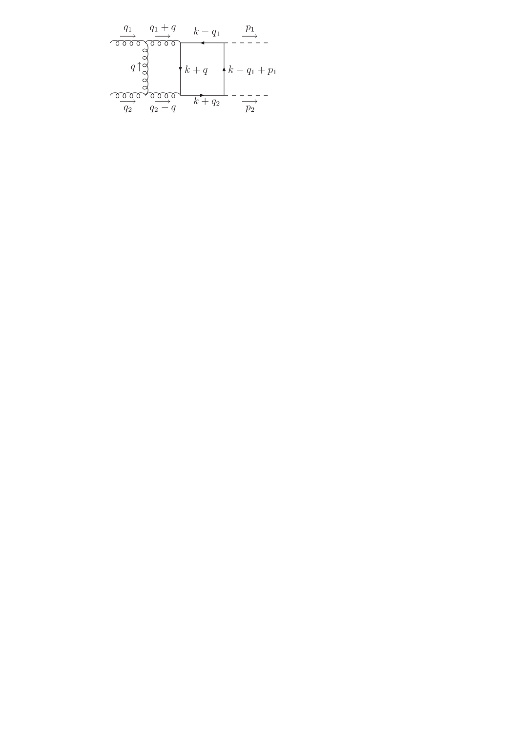
Figure 6: Explicit definitions of the virtual momenta in box 45.

Based on the distribution of the loop and external momenta of Fig. 6, the contribution to the two-loop matrix element is given by

$$A_{45}^{\mu\nu} = \frac{3}{8}\,\frac{\alpha_{s}}{\pi}\,(4\pi)^{4}\,B_{45}^{\mu\nu}\,,$$

$$B_{45}^{\mu\nu} \!\!\!=\!\!\! \int\frac{d^{n}kd^{n}q}{(2\pi)^{2n}}\frac{Tr\Big{\{}(\,\!\!\not\!{k}-\!\!\not\!{q}_{1}+m_{t})(\,\!\!\not\!{k}-\!\!\not\!{q}_{1}+\!\!\not\!{p}_{1}+m_{t})(\,\!\!\not\!{k}+\!\!\not\!{q}_{2}+m_{t})\gamma^{\sigma}(\,\!\!\not\!{k}+\!\!\not\!{q}+m_{t})\gamma^{\rho}\Big{\}}}{[(k+q)^{2}-m_{t}^{2}][(k+q_{2})^{2}-m_{t}^{2}][(k+p_{1}-q_{1})^{2}-m_{t}^{2}][(k-q_{1})^{2}-m_{t}^{2}]}$$ (53)

$$\qquad\times~{}\frac{\Big{\{}g_{\rho\tau}(2q+q_{1})^{\mu}-g^{\mu}_{\rho}(q+2q_{1})_{\tau}-g^{\mu}_{\tau}(q-q_{1})_{\rho}\Big{\}}}{(q+q_{1})^{2}(q-q_{2})^{2}q^{2}}$$

$$\qquad\times~{}\Big{\{}g^{\nu\tau}(q+q_{2})_{\sigma}+g^{\nu}_{\sigma}(q-2q_{2})^{\tau}-g_{\sigma}^{\tau}(2q-q_{2})^{\nu}\Big{\}}\,.$$

Following the same procedure as for box 39 for the Feynman parametrization, we have first performed the parametrization of the $k$-integration following the ordering of the denominator of Eq. (53). The shift in the loop momentum $k$ and the corresponding substitutions of the Feynman parameters are given by

$$k \to k-Q_{1}\,,$$

$$Q_{1} = (1-x)q-xyq_{1}+x(1-y)q_{2}+xyzp_{1}\,,$$

$$x_{1} = (1-x)\,,\quad x_{2}=x(1-y)\,,\quad x_{3}=xyz\,.$$ (54)

Performing the second loop integration over $q$ with the residual (normalized) denominator of the $k$ integration as the first propagator of the $q$ integration, attributing the additional Feynman parameters $x_{4},x_{5},x_{6}$ to the remaining propagators in Eq. (53) and applying the substitutions

$$x_{4}=rs\,,\quad x_{5}=1-s\,,\quad x_{6}=(1-r)st\,,$$ (55)

we arrive at the final expressions for the shift of $q$ and the denominator that contribute to the two form factors,

$$q \to q-Q_{2}\,,$$

$$Q_{2} = [yrs+1-s]q_{1}-[(1-y)rs+(1-r)st]q_{2}-yzrsp_{1}\,,$$

$$N(\vec{x}) = r-\rho_{s}x\Big{\{}xy(1-y)r+(1-x)[1-s+yrs][(1-r)t+(1-y)r]\Big{\}}$$ (56)

$$\quad-\rho_{t}xyzr\Big{\{}1-xy-(1-x)[yrs+1-s]\Big{\}}-\rho_{H}xyzr\Big{\{}1-xyz-(1-x)yzrs\Big{\}}$$

$$\quad-\rho_{u}xyzr\Big{\{}x(1-y)+(1-x)s[(1-r)t+(1-y)r]\Big{\}}$$

and the final integrals of the two form factors ($i=1,2$) can be cast into the form

$$\Delta F_{i}=\Gamma(1+2\epsilon)\left(\frac{4\pi\mu_{0}^{2}}{m_{t}^{2}}\right)^{2\epsilon}\int_{0}^{1}d^{6}x~{}\frac{x^{1+\epsilon}(1-x)^{\epsilon}r^{1+\epsilon}s^{-\epsilon}H_{i}(\vec{x})}{N^{3+2\epsilon}(\vec{x})}\,,$$ (57)

where $H_{i}(\vec{x})$ contains all additional regular Feynman-parameter factors from Jacobians and the normalization of the denominator of the first loop-integration over $k$. It develops a singular Laurent-expansion in $\epsilon$. The final denominator exhibits the basic form of $r+O(1/m_{t}^{2})$, so that the additional singular behavior is entirely controlled by the limit of small $r$. Since the denominator is of the form

$$N(\vec{x}) = ar^{2}+br+c\,,$$

$$\mbox{where}\qquad a = x(1-x)ys\Big{[}-\rho_{s}(1-y-t)+\rho_{t}yz-\rho_{u}z(1-y-t)+\rho_{H}yz^{2}\Big{]}\,,$$

$$b = 1-\rho_{s}x\Big{\{}xy(1-y)+(1-x)[(1-s)(1-y-t)+yst]\Big{\}}-\rho_{H}xyz(1-xyz)$$

$$-\rho_{t}xyz[1-xy-(1-x)(1-s)]-\rho_{u}xyz[x(1-y)+(1-x)st]\,,$$

$$c = -\rho_{s}x(1-x)(1-s)t$$ (58)

with $a,c={\cal O}(1/m_{t}^{2})$ and $b=1+{\cal O}(1/m_{t}^{2})$ and the infrared singularities are universal (relative to the LO expressions) the coefficient $a$ does not contribute to the infrared singularity structure, because $a$ is subleading relative to $b$ in the limit $r\to 0$. Thus, we can construct infrared subtraction terms that turn the contributions to the form factors into

$$\Delta F_{i} = \frac{\alpha_{s}}{\pi}~{}\Gamma(1+2\epsilon)\left(\frac{4\pi\mu_{0}^{2}}{m_{t}^{2}}\right)^{2\epsilon}(G_{1}+G_{2})\,,$$

$$G_{1} = \int_{0}^{1}d^{6}x~{}x^{1+\epsilon}(1-x)^{\epsilon}r^{1+\epsilon}s^{-\epsilon}\left\{\frac{H_{i}(\vec{x})}{N^{3+2\epsilon}(\vec{x})}-\frac{H_{i}(\vec{x})|_{r=0}}{N_{0}^{3+2\epsilon}(\vec{x})}\right\}\,,$$

$$G_{2} = \int_{0}^{1}d^{6}x~{}x^{1+\epsilon}(1-x)^{\epsilon}r^{1+\epsilon}s^{-\epsilon}\frac{H_{i}(\vec{x})|_{r=0}}{N_{0}^{3+2\epsilon}(\vec{x})}$$

$$\mbox{with}\qquad N_{0}(\vec{x}) = br+c\,.$$ (59)

Numerically, we have tested that the subtracted integral $G_{1}$ (after expansion in the dimensional regulator $\epsilon$) is finite for each coefficient of the expansion in $\epsilon$ individually by integrating the Feynman-parameter integrals from $\tilde{\epsilon}$ to $1-\tilde{\epsilon}$ with $\tilde{\epsilon}$ varied down to $10^{-10}$. The second integral $G_{2}$ can be integrated over the Feynman parameter $r$ analytically giving rise to hypergeometric functions,

$$G_{2}=\frac{1}{2+\epsilon}\int_{0}^{1}d^{5}x~{}\frac{x^{1+\epsilon}(1-x)^{\epsilon}s^{-\epsilon}}{c^{3+2\epsilon}}~{}_{2}F_{1}\left(3+2\epsilon,2+\epsilon;3+\epsilon;-\frac{b}{c}\right)\left.H_{i}(\vec{x})\right|_{r=0}$$ (60)

with $d^{5}x=dx\,dy\,dz\,ds\,dt$. Since this integral is singular for $c\to 0$, we have to invert the last argument of the hypergeometric function. Using the transformation relation

$$~{}_{2}F_{1}(a,b;c;z) = \frac{\Gamma(c)\Gamma(b-a)}{\Gamma(b)\Gamma(c-a)}(-z)^{-a}~{}_{2}F_{1}\left(a,1-c+a;1-b+a;\frac{1}{z}\right)$$ (61)

$$\qquad+\frac{\Gamma(c)\Gamma(a-b)}{\Gamma(a)\Gamma(c-b)}(-z)^{-b}~{}_{2}F_{1}\left(b,1-c+b;1-a+b;\frac{1}{z}\right)\,,$$

the special property

$$~{}_{2}F_{1}(a,0;c;z)=1$$ (62)

and suitable end-point subtractions of the residual singular integrals analogous to box 39, we arrive at the final decomposition of the initial Feynman-parameter integral

$$\Delta F_{i} = \frac{\alpha_{s}}{\pi}~{}\Gamma(1+\epsilon)\frac{\Gamma(1-\epsilon)}{\Gamma(1-2\epsilon)}\left(\frac{4\pi\mu_{0}^{2}}{m_{t}^{2}}\right)^{2\epsilon}\sum_{j=1}^{6}S_{j}\,,$$

$$S_{1} = \int_{0}^{1}d^{6}x~{}xr\left\{\frac{H_{i}(\vec{x})}{N^{3}(\vec{x})}\left[1+\epsilon L+\epsilon^{2}\left(\frac{L^{2}}{2}+3\zeta_{2}\right)\right]\right.$$

$$\qquad\quad-\left.\frac{H_{i}(\vec{x})|_{r=0}}{(c+br)^{3}}\left[1+\epsilon L_{0}+\epsilon^{2}\left(\frac{L_{0}^{2}}{2}+3\zeta_{2}\right)\right]\right\}\,,$$

$$S_{2} = -\int_{0}^{1}d^{6}x~{}x\frac{H_{i}(\vec{x})|_{r=0}}{(b+cr)^{3}}\left\{1+\epsilon L_{1}+\epsilon^{2}\left(\frac{L_{1}^{2}}{2}+3\zeta_{2}\right)+\epsilon^{3}\left(\frac{L_{1}^{3}}{6}+3\zeta_{2}L_{1}\right)\right\}\,,$$

$$S_{3} = -\int_{0}^{1}\frac{d^{5}x}{2\rho_{s}(1-x)(1-s)t}\left\{\frac{H_{i}(\vec{x})|_{r=0}}{b^{2}}\left[1-\epsilon(L_{2}+2)+\epsilon^{2}\left(\frac{L_{2}^{2}}{2}+2L_{2}+2\zeta_{2}+4\right)\right]\right.$$

$$\qquad\quad+\frac{H_{i}(\vec{x})|_{r,t=0,s=1}}{b_{0}^{2}}\left[1-\epsilon(L_{3}+2)+\epsilon^{2}\left(\frac{L_{3}^{2}}{2}+2L_{3}+2\zeta_{2}+4\right)\right]$$

$$\qquad\quad-\frac{H_{i}(\vec{x})|_{r=0,s=1}}{b_{1}^{2}}\left[1-\epsilon(L_{4}+2)+\epsilon^{2}\left(\frac{L_{4}^{2}}{2}+2L_{4}+2\zeta_{2}+4\right)\right]$$

$$\qquad\quad\left.-\frac{H_{i}(\vec{x})|_{r,t=0}}{b_{2}^{2}}\left[1-\epsilon(L_{5}+2)+\epsilon^{2}\left(\frac{L_{5}^{2}}{2}+2L_{5}+2\zeta_{2}+4\right)\right]\right\}\,,$$

$$S_{4} = -\int_{0}^{1}\frac{dx\,dy\,dz\,ds}{2\rho_{s}(1-x)(1-s)}\left\{\frac{H_{i}(\vec{x})|_{r,t=0}}{b_{2}^{2}}\left[-\frac{1}{\epsilon}+L_{6}+2-\epsilon\left(\frac{L_{6}^{2}}{2}+2L_{6}+2\zeta_{2}+4\right)\right.\right.$$

$$\qquad\qquad\qquad\qquad\qquad\left.+\epsilon^{2}\left(\frac{L_{6}^{3}}{6}+L_{6}^{2}+2(\zeta_{2}+2)L_{6}-2\zeta_{3}+4\zeta_{2}+8\right)\right]$$

$$\qquad\quad-\frac{H_{i}(\vec{x})|_{r,t=0,s=1}}{b_{0}^{2}}\left[-\frac{1}{\epsilon}+L_{7}+2-\epsilon\left(\frac{L_{7}^{2}}{2}+2L_{7}+2\zeta_{2}+4\right)\right.$$

$$\qquad\qquad\qquad\qquad\qquad\left.\left.+\epsilon^{2}\left(\frac{L_{7}^{3}}{6}+L_{7}^{2}+2(\zeta_{2}+2)L_{7}-2\zeta_{3}+4\zeta_{2}+8\right)\right]\right\}\,,$$

$$S_{5} = -\int_{0}^{1}\frac{dx\,dy\,dz\,dt}{2\rho_{s}(1-x)t}\left\{\frac{H_{i}(\vec{x})|_{r=0,s=1}}{b_{1}^{2}}\left[-\frac{1}{\epsilon}+L_{8}+2-\epsilon\left(\frac{L_{8}^{2}}{2}+2L_{8}+\zeta_{2}+4\right)\right.\right.$$

$$\qquad\qquad\qquad\qquad\qquad\left.+\epsilon^{2}\left(\frac{L_{8}^{3}}{6}+L_{8}^{2}+(\zeta_{2}+4)L_{8}+2\zeta_{2}+8\right)\right]$$

$$\qquad\quad-\frac{H_{i}(\vec{x})|_{r,t=0,s=1}}{b_{0}^{2}}\left[-\frac{1}{\epsilon}+L_{9}+2-\epsilon\left(\frac{L_{9}^{2}}{2}+2L_{9}+\zeta_{2}+4\right)\right.$$

$$\qquad\qquad\qquad\qquad\qquad\left.\left.+\epsilon^{2}\left(\frac{L_{9}^{3}}{6}+L_{9}^{2}+(\zeta_{2}+4)L_{9}+2\zeta_{2}+8\right)\right]\right\}\,,$$

$$S_{6} = -\int_{0}^{1}dx\,dy\,dz~{}\frac{H_{i}(\vec{x})|_{r,t=0,s=1}}{2\rho_{s}(1-x)b_{0}^{2}}\left\{\frac{1}{\epsilon^{2}}-\frac{1}{\epsilon}(L_{10}+2)+\frac{L_{10}^{2}}{2}+2L_{10}+\zeta_{2}+4\right.$$ (63)

$$\qquad\qquad\qquad\qquad\qquad\left.-\epsilon\left(\frac{L_{10}^{3}}{6}+L_{10}^{2}+(\zeta_{2}+4)L_{10}+2\zeta_{2}+8\right)\right\}\,.$$

The logarithms used in the expressions above are defined as

$$L = \log\left(\frac{x(1-x)r}{s}\right)-2\log N\,,\qquad\qquad\qquad\,L_{0}=\log\left(\frac{x(1-x)r}{s}\right)-2\log(c+br)\,,$$

$$L_{1} = \log\left(\frac{x(1-x)r}{s}\right)-2\log(b+cr)\,,\qquad\qquad L_{2}=\log\left[-\rho_{s}s(1-s)t\right]+\log b\,,$$

$$L_{3} = \log\left[-\rho_{s}s(1-s)t\right]+\log b_{0}\,,\qquad\qquad\qquad\ \ \,L_{4}=\log\left[-\rho_{s}s(1-s)t\right]+\log b_{1}\,,$$

$$L_{5} = \log\left[-\rho_{s}s(1-s)t\right]+\log b_{2}\,,\qquad\qquad\qquad\ \ \,L_{6}=\log\left[-\rho_{s}s(1-s)\right]+\log b_{2}\,,$$

$$L_{7} = \log\left[-\rho_{s}s(1-s)\right]+\log b_{0}\,,\qquad\qquad\qquad\quad\,L_{8}=\log\left(-\rho_{s}t\right)+\log b_{1}\,,$$

$$L_{9} = \log\left(-\rho_{s}t\right)+\log b_{0}\,,\qquad\qquad\qquad\qquad\qquad\!\!L_{10}=\log\left(-\rho_{s}\right)+\log b_{0}$$ (64)

and the remaining objects $b_{0},b_{1},b_{2}$ as

$$b_{0} = b|_{t=0,s=1}\,,\qquad\qquad b_{1}=b|_{s=1}\,,\qquad\qquad b_{2}=b|_{t=0}$$ (65)

with $b$ from Eq. (58).

Box 45 contains a second threshold for $Q^{2}>0$ so that even below the $t\bar{t}$-threshold, integrations by parts are required to stabilize the integrand numerically. These integrations by parts are performed for the Feynman parameter $r$ in the contributions $S_{1,2}$ along the same lines as for box 39, while the integrals $S_{3-6}$ are stable without integrations by parts.

3.1.4 Renormalization

The strong coupling $\alpha_{s}$ has been renormalized in the $\overline{\rm MS}$ scheme with the top quark decoupled, i.e. the renormalization constant is given by

$$\alpha_{s,0} = \alpha_{s}(\mu_{R})+\delta\alpha_{s}\,,$$

$$\frac{\delta\alpha_{s}}{\alpha_{s}} = \frac{\alpha_{s}}{\pi}\Gamma(1+\epsilon)\left(\frac{4\pi\mu_{0}^{2}}{\mu_{R}^{2}}\right)^{\epsilon}\left\{-\frac{33-2(N_{F}+1)}{12\epsilon}+\frac{1}{6}\log\frac{\mu_{R}^{2}}{m_{t}^{2}}\right\}$$ (66)

with $N_{F}=5$. This choice ensures that there are no artificial large logarithms of the top mass for the available energy range of the LHC in the final result, since we do not introduce top densities inside the proton, i.e. work in a five-flavour scheme. The additional logarithm of the top mass cancels against the diagrams with a top loop within the external gluon lines, see Fig. 7. This leads to the total contribution related to the renormalization of the strong coupling

$$\delta_{\alpha_{s}}F_{i}=\frac{\alpha_{s}}{\pi}\Gamma(1+\epsilon)\left(\frac{4\pi\mu_{0}^{2}}{\mu_{R}^{2}}\right)^{\epsilon}\left\{-\frac{33-2N_{F}}{12\epsilon}\right\}F_{i,LO}\,,$$ (67)

where the LO form factors $F_{i}$ have to be used in $n$ dimensions, i.e. including higher orders in the dimensional regulator $\epsilon$.

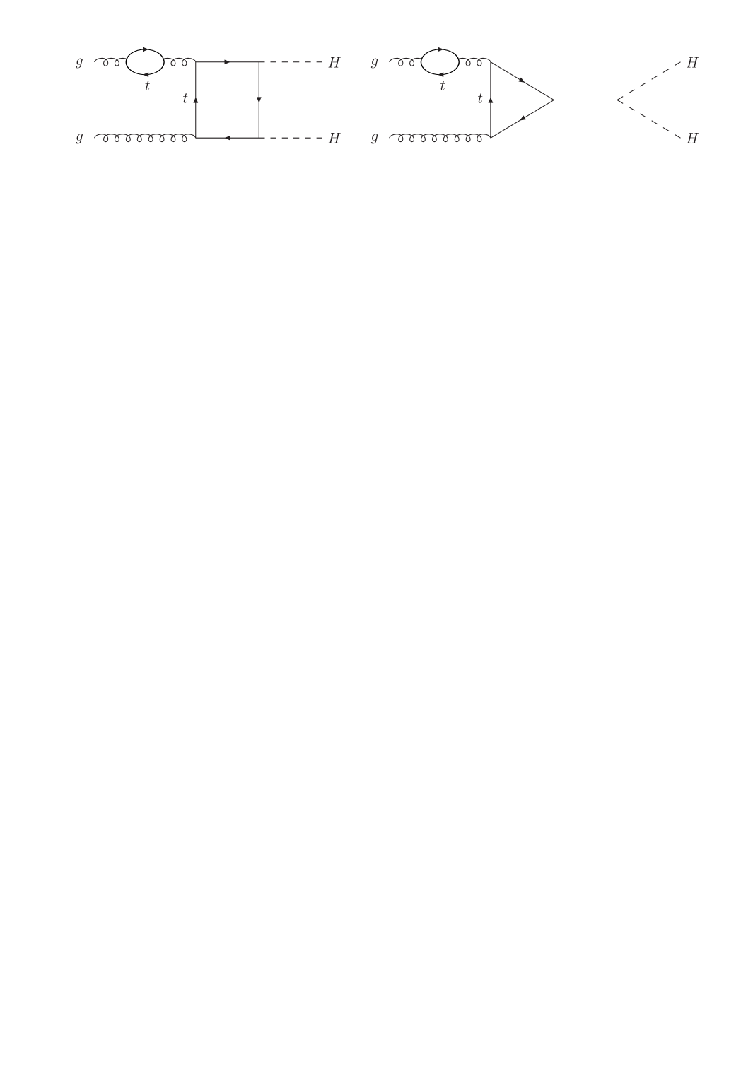
Figure 7: Typical diagrams with external top loops.

For our default prediction, we have renormalized the top mass on-shell so that the renormalization constant is given by

$$m_{t,0} = m_{t}-\delta m_{t}\,,$$

$$\frac{\delta m_{t}}{m_{t}} = \frac{\alpha_{s}}{\pi}\Gamma(1+\epsilon)\left(\frac{4\pi\mu_{0}^{2}}{m_{t}^{2}}\right)^{\epsilon}\left\{\frac{1}{\epsilon}+\frac{4}{3}\right\}\,.$$ (68)

The explicit contribution of the mass counterterm can either be obtained by calculating the corresponding counterterm diagrams or, in much more elegant manner, by differentiating the LO form factors with respect to the top mass,

$$\delta_{m_{t}}F_{i}=-\delta m_{t}\frac{\partial F_{i,LO}}{\partial m_{t}}\,,$$ (69)

where we followed the second option. For the renormalization of the top mass in terms of the $\overline{\rm MS}$ mass, a counterterm

$$m_{t,0} = \overline{m}_{t}(\mu_{t})-\delta\overline{m}_{t}\,,$$

$$\frac{\delta\overline{m}_{t}}{\overline{m}_{t}(\mu_{t})} = \frac{\alpha_{s}}{\pi}\Gamma(1+\epsilon)\left(\frac{4\pi\mu_{0}^{2}}{\mu_{t}^{2}}\right)^{\epsilon}\frac{1}{\epsilon}$$ (70)

has to be used with the LO and NLO expressions of the form factors expressed in terms of the $\overline{\rm MS}$ top mass $\overline{m}_{t}(\mu_{t})$. For the evaluation of the $\overline{\rm MS}$ top mass, we use the N³LO relation between the pole and $\overline{\rm MS}$ mass Gray:1990yh ; Chetyrkin:1999ys ; Chetyrkin:1999qi ; Melnikov:2000qh ,

$${\overline{m}}_{t}(m_{t}) = \frac{m_{t}}{\displaystyle 1+\frac{4}{3}\frac{\alpha_{s}(m_{t})}{\pi}+K_{2}\left(\frac{\alpha_{s}(m_{t})}{\pi}\right)^{2}+K_{3}\left(\frac{\alpha_{s}(m_{t})}{\pi}\right)^{3}}$$ (71)

with $K_{2}\approx 10.9$ and $K_{3}\approx 107.11$. The scale dependence of the $\overline{\rm MS}$ mass is treated at N³LL,

$${\overline{m}}_{t}\,(\mu_{t}) = {\overline{m}}_{t}\,(m_{t})\,\frac{c\,[\alpha_{s}\,(\mu_{t})/\pi]}{c\,[\alpha_{s}\,(m_{t})/\pi]}$$ (72)

with the coefficient function Tarasov:1982gk ; Chetyrkin:1997dh

$$c(x)=\left(\frac{7}{2}\,x\right)^{\frac{4}{7}}\,[1+1.398x+1.793\,x^{2}-0.6834\,x^{3}]\,.$$ (73)

Since we are interested in the finite top-mass effects on top of the LO ones, we have subtracted in addition the Born-improved HTL of the virtual corrections involving the full top-mass dependence at LO Dawson:1998py . This yields the additional subtraction term

$$\delta_{HTL}F_{i}=\frac{\alpha_{s}}{\pi}\frac{\Gamma(1-\epsilon)}{\Gamma(1-2\epsilon)}\left(\frac{4\pi\mu_{0}^{2}}{-m_{t}^{2}\rho_{s}}\right)^{\epsilon}\left\{\frac{3}{2\epsilon^{2}}+\frac{33-2N_{F}}{12\epsilon}\left(\frac{\mu_{R}^{2}}{-m_{t}^{2}\rho_{s}}\right)^{-\epsilon}-\frac{11}{4}+\frac{\pi^{2}}{4}\right\}F_{i,LO}\,.$$ (74)

After adding this subtraction term, the result of Hpair can simply be added back to the NLO top-mass effects obtained in this way for the virtual corrections. Thus, the total counterterm plus HTL-subtraction is given by

$$\delta F_{i}=\delta_{\alpha_{s}}F_{i}+\delta_{m_{t}}F_{i}+\delta_{HTL}F_{i}\,.$$ (75)

The addition of this term results in an infrared and ultraviolet finite result for the virtual corrections as we have explicitly checked numerically. It should be noted that we have defined this total subtraction term with the imaginary part $\bar{\epsilon}$ for the top mass to be consistent with our treatment of the two-loop diagrams. For the two-loop triangle diagrams, this total subtraction term is included in the narrow-width approximation according to the known result for the single-Higgs case.

3.1.5 Differential cross section

The final numerical integrations have been performed by Vegas Lepage:1980dq for the differential cross sections $d\sigma/dQ^{2}$ of Eq. (20), i.e. the integration over $\hat{t}$ is included. Each individual box diagram is divergent in $\hat{t}$ at the lower and upper bound of the $\hat{t}$-integration in general. To stabilize the $\hat{t}$-integration, we have performed a suitable substitution to smoothen the integrand,

$$\hat{t}_{1}=m_{t}^{2}e^{y}+t_{1-}$$ (76)

with $\hat{t}_{1}=\hat{t}-M_{H}^{2},\hat{u}_{1}=\hat{u}-M_{H}^{2}$ and $\hat{t}_{1\pm}=\hat{t}_{\pm}-M_{H}^{2}$, where the integration boundaries $\hat{t}_{\pm}$ are given in Eq. (14). By means of this substitution, we can rewrite the integration over $\hat{t}_{1}$ generically as

$$\int_{\hat{t}_{1-}}^{\hat{t}_{1+}}\frac{d\hat{t}_{1}}{\hat{t}_{1}\hat{u}_{1}-\hat{s}M_{H}^{2}}f(\hat{t}_{1},\hat{u}_{1})=\int_{y_{-}}^{y_{+}}\frac{dy}{t_{+}-t_{-}}\Big{[}f(\hat{t}_{1},\hat{u}_{1})+f(\hat{u}_{1},\hat{t}_{1})\Big{]}\,,$$ (77)

where $f(\hat{t}_{1},\hat{u}_{1})$ denotes the corresponding virtual matrix element with the (singular) denominator $\hat{t}_{1}\hat{u}_{1}-\hat{s}M_{H}^{2}$ extracted and the integration boundaries read

$$y_{+} = \log\frac{(t_{+}-t_{-})(1-\tilde{\epsilon})}{m_{t}^{2}}\,,$$

$$y_{-} = \log\frac{(t_{+}-t_{-})\tilde{\epsilon}}{m_{t}^{2}}\,,$$ (78)

where we have introduced a cut $\tilde{\epsilon}$ for the upper and lower bound of the $\hat{t}_{1}$-integration (after rewriting this into an integral from 0 to 1 and replacing these integration boundaries by $\tilde{\epsilon}$ and $1-\tilde{\epsilon}$). We have checked that the total sum of all box diagrams becomes independent of this cut by varying $\tilde{\epsilon}$ down to $10^{-10}$, i.e. that the total sum is again finite.

3.2 Real corrections

We are left with the evaluation of the real contributions to complete the picture of the NLO QCD corrections. As we are interested in the calculation of the top-mass effects on top of the HTL calculation that is provided by Hpair, we use the universality of the infrared divergent pieces to subtract the Born-improved HTL contributions $d\sigma_{ij}^{\text{HTL}}$ in such a way that our integration of the real contributions $d\Delta\sigma_{ij}^{\text{mass}}=d\sigma_{ij}-d\sigma_{ij}^{\text{HTL}}$ is finite. We construct a local subtraction term for the partonic channels $d\hat{\sigma}_{ij}$,

$$d\Delta\hat{\sigma}^{\text{mass}}_{ij}(p_{k})=d\hat{\sigma}_{ij}(p_{k})-d\hat{\sigma}_{\text{LO}}(\tilde{p}_{k})\frac{d\hat{\sigma}_{ij}^{\text{HTL}}(p_{k})}{d\hat{\sigma}_{\text{LO}}^{\text{HTL}}(\tilde{p}_{k})},$$ (79)

where $p_{k}$ denote the four-momenta from the full $2\to 3$ phase-space and $\tilde{p}_{k}$ stand for the mapping of the momenta $p_{k}$ on a $2\to 2$ sub-phase-space. As the results in the HTL limit are given in the Born-improved approximation in which the pure HTL is rescaled with the full LO matrix elements, we need to map the full $2\to 3$ phase-space onto a projected $2\to 2$ phase-space to construct the subtraction term involving this rescaling to the full LO contribution $d\hat{\sigma}_{\text{LO}}$.

The mapping is done by using the transformation formulae for initial-state emitter and initial-state spectator in the construction of dipole subtraction terms, i.e. using Eqs. (5.137-5.139) of Ref. Catani:1996vz . The (mapped) momenta of the initial-state partons are $p_{1/2}$ ($\tilde{p}_{1/2}$), the (mapped) momenta of the final-state Higgs bosons are $p_{3/4}$ ($\tilde{p}_{3/4}$), and the momentum of the radiated parton is $p_{5}$. For the initial-state partons, we use the following mapping,

$$\tilde{p}_{1}=p_{1},\qquad\tilde{p}_{2}=p_{2}\left(1-\frac{(p_{5}p_{1})+(p_{5}p_{2})}{(p_{1}p_{2})}\right).$$ (80)

In order to transform the Higgs momenta, we introduce the variables $K$ and $\tilde{K}$,

$$K=p_{1}+p_{2}-p_{5},\qquad\tilde{K}=\tilde{p}_{1}+\tilde{p}_{2}$$ (81)

allowing us to define

$$\tilde{p}_{3} =p_{3}-2\,\frac{p_{3}(K+\tilde{K})}{(K+\tilde{K})^{2}}\left(K+\tilde{K}\right)+2\,\frac{(p_{3}K)}{K^{2}}\tilde{K},$$

$$\tilde{p}_{4} =p_{4}-2\,\frac{p_{4}(K+\tilde{K})}{(K+\tilde{K})^{2}}\left(K+\tilde{K}\right)+2\,\frac{(p_{4}K)}{K^{2}}\tilde{K}.$$ (82)

The HTL matrix elements are calculated analytically. We introduce the partonic center-of-mass energy $\hat{s}$, and the Mandelstam variables $\hat{t}=(p_{1}-p_{5})^{2}$ and $\hat{u}=(p_{2}-p_{5})^{2}$. The invariant squared Higgs-pair mass is $Q^{2}=\hat{s}+\hat{t}+\hat{u}$. The real spin- and colour-averaged matrix elements are

$$\overline{\Big{|}\mathcal{M}_{gg\to HHg}^{\text{HTL}}\Big{|}^{2}} =\frac{\alpha_{s}^{3}(\mu_{R})G_{F}^{2}}{12\pi}\,\frac{\hat{s}^{4}+\hat{t}^{4}+\hat{u}^{4}+Q^{8}}{\hat{s}\hat{t}\hat{u}}\left(1-\frac{3M_{H}^{2}}{Q^{2}-M_{H}^{2}}\right)^{2},$$

$$\overline{\Big{|}\mathcal{M}_{qg\to HHq}^{\text{HTL}}\Big{|}^{2}} =\frac{\alpha_{s}^{3}(\mu_{R})G_{F}^{2}}{27\pi}\,\frac{\hat{s}^{2}+\hat{u}^{2}}{-\hat{t}}\left(1-\frac{3M_{H}^{2}}{Q^{2}-M_{H}^{2}}\right)^{2},$$

$$\overline{\Big{|}\mathcal{M}_{q\bar{q}\to HHg}^{\text{HTL}}\Big{|}^{2}} =\frac{8\alpha_{s}^{3}(\mu_{R})G_{F}^{2}}{81\pi}\,\frac{\hat{t}^{2}+\hat{u}^{2}}{\hat{s}}\left(1-\frac{3M_{H}^{2}}{Q^{2}-M_{H}^{2}}\right)^{2},$$ (83)

and the LO matrix element in the HTL reads

$$\overline{\Big{|}\mathcal{M}_{\text{LO}}^{\text{HTL}}\Big{|}^{2}}=\frac{\alpha_{s}^{2}(\mu_{R})G_{F}^{2}}{288\pi^{2}}\,Q^{4}\left(1-\frac{3M_{H}^{2}}{Q^{2}-M_{H}^{2}}\right)^{2}.$$ (84)

The full one-loop matrix elements have been generated with FeynArts Hahn:2000kx and FormCalc Hahn:1998yk . They contain triangle, box, and pentagons diagrams. Generic diagrams for the contribution $gg\to HHg$ are given in Fig. 8, generic diagrams for the contributions $qg\to HHq$ and $q\bar{q}\to HHg$ are displayed in Fig. 9. The numerical evaluation of the scalar integrals tHooft:1978jhc as well as the tensor reduction has been performed using the techniques developed in Refs. vanOldenborgh:1990yc ; Denner:2002ii ; Denner:2005nn ; Denner:2010tr and implemented in the library Collier 1.2 Denner:2016kdg . The latter has been interfaced to the analytic expressions generated by FormCalc with an in-house routine. In order to improve our numerical stability, we have implemented a technical collinear cut in the phase-space parametrization. The integration of the scattering angle $\theta$ of the radiated parton in the c.m. system is restricted to the range $|\!\cos\theta|<1-\delta$ with $\delta=10^{-4}$. We have checked that our results are stable against a variation of $\delta$ from $10^{-4}$ to $10^{-6}$ and therefore they are not affected by our choice for this technical cut.

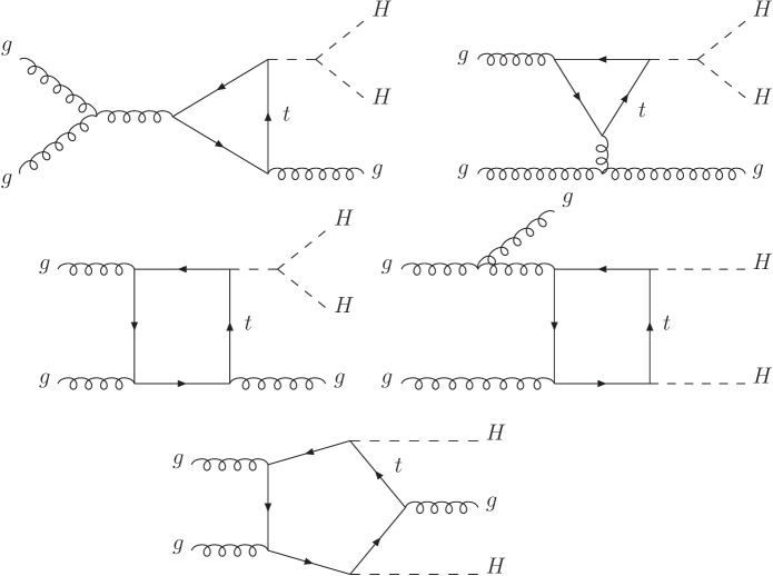
Figure 8: Typical one-loop triangle (upper row), box (middle row), and pentagon (lower row) diagrams for the partonic channel $gg\to HHg$ contributing to the real corrections of Higgs-pair production via gluon fusion at NLO in QCD.

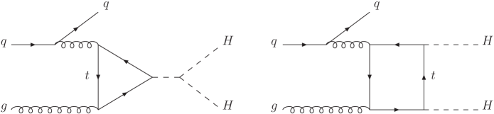
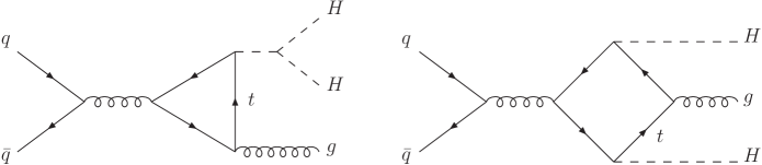
Figure 9: Typical one-loop triangle and box diagrams for the partonic channels $qg\to HHq$ (upper row) and $q\bar{q}\to HHg$ (lower row), contributing to the real corrections of Higgs-pair production via gluon fusion at NLO in QCD.

We have cross-checked the final mass-effects of the real corrections against the results presented in the literature Frederix:2014hta ; Maltoni:2014eza ; Borowka:2016ehy ; Borowka:2016ypz and we have obtained agreement.

4 Results

Our numerical results will be presented for the invariant Higgs-pair-mass distributions for different c.m. energies, i.e. 14 TeV for the LHC, 27 TeV for a potential high-energy LHC (HE-LHC) and 100 TeV for a provisional proton collider within the Future-Circular-Collider (FCC) project. The Higgs mass has been chosen as $M_{H}=125$ GeV and the top pole mass as $m_{t}=172.5$ GeV. The results for the full NLO cross sections have been obtained with two different PDF sets, MMHT2014 Harland-Lang:2014zoa and PDF4LHC15 Butterworth:2015oua , that are taken from the LHAPDF-6 library Buckley:2014ana . The central scale choices for the renormalization and factorization scales are $\mu_{F}=\mu_{R}=Q/2$ and the input value $\alpha_{s}(M_{Z})$ is chosen according to the PDF set used. Since MMHT2014 contains a LO set, these PDFs are used for the evaluation of the consistent K-factors with the NLO (LO) cross section calculated with NLO (LO) $\alpha_{s}$ and PDFs. The whole calculation of the virtual and real corrections has been performed at least twice independently adopting also different Feynman parametrizations of the virtual two-loop diagrams. The real corrections have been derived with different parametrizations of the real phase-space. Both calculations agree within the numerical errors. We work in the narrow-width approximation of the top quark so that the Richardson extrapolation has to be applied to reach this limit for the two-loop box diagrams..

4.1 Differential cross section

For the differential cross section, we have computed a grid of $Q$-values from 250 GeV to 1.5 TeV. In order to get a reliable result for the total cross section later on, we have used steps of 5 GeV between $Q=250$ GeV and $Q=300$ GeV, steps of 25 GeV between $Q=300$ GeV and $Q=700$ GeV, and steps of 50 GeV for $Q>700$ GeV. After applying the integrations by parts to each individual virtual diagram, we reached reliable results of our numerical integrations for $\bar{\epsilon}$ values [see Eq. (34)] down to about 0.05. In order to obtain the result in the narrow-width approximation ($\bar{\epsilon}\to 0$), we have performed a Richardson extrapolation applied to the results for different values of $\bar{\epsilon}$. We adopt $\bar{\epsilon}$ values $\bar{\epsilon}_{n}=0.025\times 2^{n}$ ($n=0\dots 10$). For bins close to threshold, $Q=300,325,350$ GeV, we use the set $n=0\dots 8$. For $Q\in[375,475]$ GeV, we use $n=1\dots 9$ while we use $n=2\dots 10$ for Q values in the range $Q\in[500,700]$ GeV. For $Q$ values starting at 750 GeV, we restrict the extrapolation to $n=2\dots 6$. In this way, we obtain a series of extrapolated results up to the ninth order in the dominant region and up to the fifth order in the tails for large $Q$. We define an estimate of the theoretical error due to the Richardson extrapolation as the difference of the extrapolated results at fifth and fourth order. In addition, we multiply this error by a factor of two close to the virtual $t\bar{t}$ threshold in order to be conservative. The total estimated Richardson-extrapolation error ranges below the per-cent level and is added in quadrature to the statistical integration error.

Since we have subtracted the (Born-improved) HTL consistently from the virtual and real corrections, we are left with the pure top-mass effects at NLO that are infrared and ultraviolet finite individually after renormalization. This part has then been added to the results of Hpair hpair to derive the full NLO cross section. The final invariant Higgs-pair-mass distributions are displayed in Figs. 10–12 for the three c.m. energies, 14, 27, 100 TeV. The blue curves show the Born-improved result in the HTL of Ref. Dawson:1998py as implemented in Hpair hpair , the yellow ones the Born-improved HTL result plus the mass effects of the real corrections, the green curves the Born-improved HTL result plus the mass effects of the virtual corrections and the red curves the full NLO results. The plots on the left side of each figure have been obtained by using MMHT2014 PDFs Harland-Lang:2014zoa and the ones on the right with PDF4LHC PDFs Butterworth:2015oua . The lower panel on the left shows the consistently defined K-factors $K=d\sigma_{NLO}/d\sigma_{LO}$. The lower panel on the right shows the ratio of the differential NLO cross section to the one obtained in the Born-improved HTL.

While the Born-improved HTL provides a reasonable approximation for $Q$-values close to threshold, the real corrections add a negative mass effect of about $-10\%$ for $\sqrt{s}=14$ TeV (yellow curves) that is approximately uniform in the entire $Q$ range. The (negative) mass effects of the virtual corrections (green curves), however, become large at large values of $Q$ reaching a level of more than 20% for $Q$ beyond about 1 TeV. While the relative mass effects of the virtual corrections at NLO are independent of the collider energy (see the right plots showing the ratios to the HTL in the lower panels) in agreement with Eq. (20), the NLO mass effects of the real corrections become larger with rising collider energy, reaching a level of $-20\%$ for $\sqrt{s}=100$ TeV. Both mass effects of the virtual and real corrections add up in the same direction and result in a total modification of the differential cross section of up to $-40\%$ compared to the Born-improved HTL at large $Q$ values for $\sqrt{s}=100$ TeV. While (as for the ratios) the full NLO K-factors shown in the left plots are close to the Born-improved HTL (blue curves) at $Q$ values close to the production threshold, they deviate significantly at larger values of $Q$ due to the additional NLO top-mass effects that decrease the total size of the NLO QCD corrections compared to the HTL as expected from unitarity arguments.

To estimate the theoretical uncertainties, we have varied the renormalization and factorization scales for each bin in $Q$ by a factor of 2 up and down around the central scale $\mu_{R}=\mu_{F}=Q/2$ and derived the envelope of a 7-point variation, i.e. excluding points where the renormalization and factorization scales differ by more than a factor of two. The residual uncertainties are shown by the red band around the full NLO results (red curves) in Figs. 10–12. They range at the level of 10–15% in total as can be inferred from the explicit numbers for $\sqrt{s}=14$ TeV (using PDF4LHC PDFs),

$$\frac{d\sigma_{NLO}}{dQ}\Big{|}_{Q=300~{}{\rm GeV}} = 0.02978(7)^{+15.3\%}_{-13.0\%}\ {\rm fb/GeV},$$

$$\frac{d\sigma_{NLO}}{dQ}\Big{|}_{Q=400~{}{\rm GeV}} = 0.1609(4)^{+14.4\%}_{-12.8\%}\ {\rm fb/GeV},$$

$$\frac{d\sigma_{NLO}}{dQ}\Big{|}_{Q=600~{}{\rm GeV}} = 0.03204(9)^{+10.9\%}_{-11.5\%}\ {\rm fb/GeV},$$

$$\frac{d\sigma_{NLO}}{dQ}\Big{|}_{Q=1200~{}{\rm GeV}} = 0.000435(4)^{+7.1\%}_{-10.6\%}\ {\rm fb/GeV}\,.$$ (85)

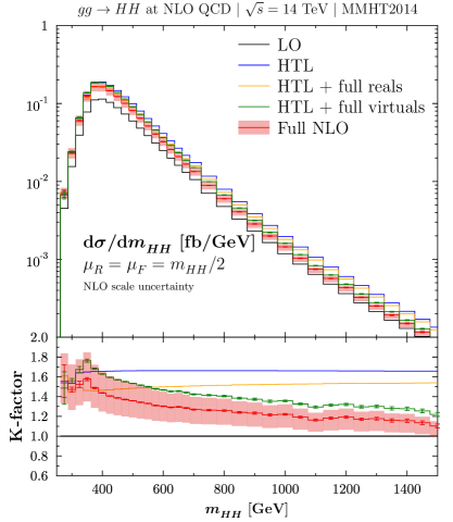
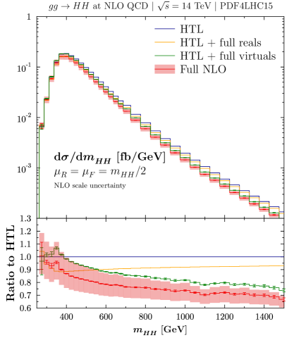
Figure 10: Invariant Higgs-pair-mass distributions for Higgs boson pair production via gluon fusion at the 14 TeV LHC as a function of $Q=m_{HH}$. LO results (in black), HTL results (in blue), HTL results including the full real corrections (in yellow), HTL results including the full virtual corrections (in green, including the numerical errors), and the full NLO QCD results (in red, including the numerical errors). Left: Results with the MMHT2014 PDF set, the panel below displays the K-factors for the different results. Right: Results with the PDF4LHC15 PDF set, the panel below displays the ratio to the NLO Born-improved HTL result for the different calculations. The red band indicates the renormalization and factorization scale uncertainties for results including the full NLO QCD corrections.

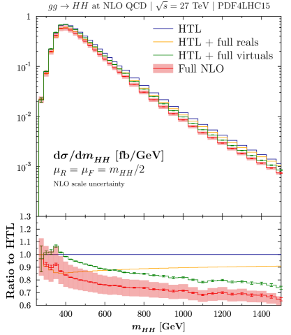
Figure 11: Same as Fig. 10 but for a c.m. energy $\sqrt{s}=27$ TeV.

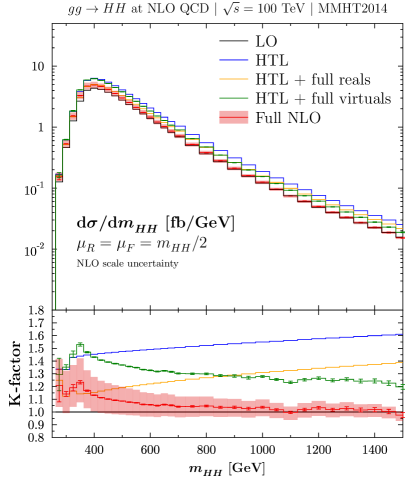
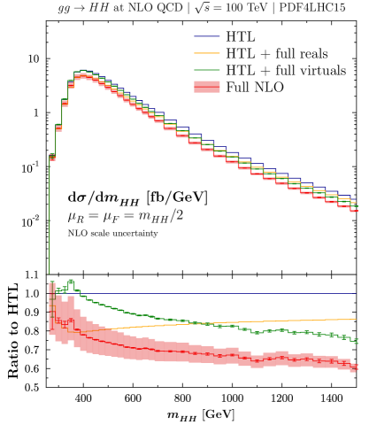
Figure 12: Same as Fig. 10 but for a c.m. energy $\sqrt{s}=100$ TeV.

We have analyzed the structure of the NLO QCD corrections in more detail by comparing the K-factor with the one of the triangle diagrams alone, i.e. with the K-factor of single-Higgs production with mass $M_{H}=Q$, in all individual approximations. This will determine the amount of universal NLO top-mass effects, common in the triangle and box diagrams. We define the ratio of the NLO triangle-diagram K-factor to the one including all diagrams as K-fac^△/K-fac. This is shown, as a function of $Q=m_{HH}$, in Fig. 13 (left). It is visible that the triangle-diagram K-factor provides an acceptable approximation to the full NLO K-factor only for $Q$ values below about 500–600 GeV if maximal deviations of about 15% are allowed (red histogram). The break down into the different mass effects of the virtual (green histogram) and real (yellow histogram) corrections singles out the origin of non-universal mass effects in the virtual corrections, while the non-universal mass effects beyond the single-Higgs case of the real corrections are limited to less than about 5% (apart from the virtual $t\bar{t}$-threshold region). In comparison to the contribution of the triangle diagrams alone, we also present the ratio of the K-factor obtained by including only the continuum diagrams (box diagrams of the virtual corrections and all box and pentagon diagrams of the real corrections without trilinear Higgs couplings) to the full K-factor in Fig. 13 (right). The different curves show the results for the various approximations, i.e. the blue curves for the Born-improved HTL, the yellow ones with the inclusion of the NLO mass effects of the real corrections, the green curves with only the virtual NLO mass effects and the red curves the full NLO results. The right figure shows that the full NLO K-factor (red curve) is well-described (within 5%) by the one for the continuum diagrams alone which coincides with the observation that the continuum diagrams play a significant role for small values of $Q$ (where the K-factor does not deviate much from the single-Higgs case) and are dominant for large $Q$. This result shows that the K-factor cannot be approximated well by the one of single-Higgs production for large values of $Q$ due to the large mass effects of the virtual corrections.

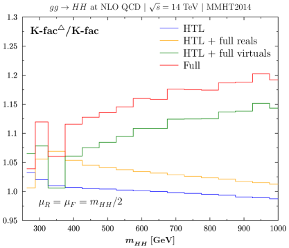
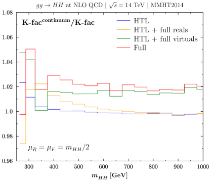
Figure 13: Ratios of the K-factor including (left) only triangle diagrams and (right) only continuum diagrams to the full K-factor of Higgs-pair production as a function of the invariant Higgs-pair mass $Q=m_{HH}$ for the LHC with a c.m. energy $\sqrt{s}=14$ TeV and using MMHT2014 parton densities.

4.2 Total cross section

The total cross section has been obtained from the invariant Higgs-pair mass distribution by means of a numerical integration of the bins in $Q$ with the trapezoidal method for $Q>300$ GeV. For a reliable result, we used a Richardson extrapolation Richardson in terms of the bin size in $Q$ also for this step. For $Q<300$ GeV, we have adopted the extension of Boole’s rule to six nodes Abramowitz . We obtain the following values for the total cross section at various c.m. energies,

$$\sqrt{s}=13~{}{\rm TeV}:\quad\sigma_{tot} = 27.73(7)^{+13.8\%}_{-12.8\%}~{}{\rm fb},$$

$$\sqrt{s}=14~{}{\rm TeV}:\quad\sigma_{tot} = 32.81(7)^{+13.5\%}_{-12.5\%}~{}{\rm fb},$$

$$\sqrt{s}=27~{}{\rm TeV}:\quad\sigma_{tot} = 127.0(2)^{+11.7\%}_{-10.7\%}~{}{\rm fb},$$

$$\sqrt{s}=100~{}{\rm TeV}:\quad\sigma_{tot} = 1140(2)^{+10.7\%}_{-10.0\%}~{}{\rm fb},$$ (86)

where we have used the PDF4LHC parton densities with $\alpha_{s}(M_{Z})=0.118$ and added for completeness also the value for a c.m. energy of 13 TeV. The numbers in brackets show the numerical errors, while the upper and lower per-centage entries determine the (asymmetric) renormalization and factorization scale dependences. The corresponding results in the Born-improved HTL with PDF4LHC PDFs, obtained with the program Hpair hpair , read

$$\sqrt{s}=13~{}{\rm TeV}:\quad\sigma_{HTL} = 32.51^{+18\%}_{-15\%}~{}{\rm fb},$$

$$\sqrt{s}=14~{}{\rm TeV}:\quad\sigma_{HTL} = 38.65^{+18\%}_{-15\%}~{}{\rm fb},$$

$$\sqrt{s}=27~{}{\rm TeV}:\quad\sigma_{HTL} = 156.2^{+17\%}_{-13\%}~{}{\rm fb},$$

$$\sqrt{s}=100~{}{\rm TeV}:\quad\sigma_{HTL} = 1521^{+16\%}_{-13\%}~{}{\rm fb}.$$ (87)

Comparing the results of Eqs. (86) and (87), we observe a reduction of the total cross section by about 15% due to the top-mass effects at NLO and a reduction of the scale uncertainty. These numbers, as well as the differential distributions presented in Section 4.1, agree with the results of Refs. Borowka:2016ehy ; Borowka:2016ypz . It should be noted that a comparison of the full virtual corrections with the analytical large top-mass expansion presented in Ref. Grigo:2015dia was performed in Refs. Borowka:2016ehy ; Borowka:2016ypz and shows a convergence to the full result below the $t\bar{t}$-threshold, as expected.

4.3 Uncertainties originating from the top-mass definition

An uncertainty that has been neglected or underestimated often previously is the intrinsic uncertainty due to the scheme and scale choice of the virtual top mass. This does not play a large role for single on-shell Higgs-boson production via gluon fusion, $gg\to H$, since the Higgs mass is small and thus the HTL works well, i.e. top-mass effects are suppressed. This uncertainty, however, plays a significant role for the larger values of $Q$ in Higgs-pair production. Top-mass effects are already sizeable at LO, but the NLO corrections add additional relevant top-mass dependences on top of the LO result as we have discussed in the previous subsection. The top mass is a scheme and scale dependent quantity so that the related uncertainties need to be estimated for a reliable determination of the total theoretical uncertainties. For this analysis, we have evaluated the differential cross section for the top mass defined in the on-shell scheme (default) and in the $\overline{\rm MS}$-scheme at the scale $\mu_{t}$, i.e. adjusting the counterterms and input parameters to the choices $\overline{m}_{t}(\overline{m}_{t})$ and $\overline{m}_{t}(\mu_{t})$ with $\mu_{t}$ in the range between $Q/4$ and $Q$ according to Section 3.1.4. Since the scale dependence on $\mu_{t}$ is a monotonously falling function, we evaluated the differential cross section for four choices of the top mass, $m_{t}$, $\overline{m}_{t}(\overline{m}_{t})$, $\overline{m}_{t}(Q/4)$ and $\overline{m}_{t}(Q)$, for each bin in $Q$.

For the three c.m. energies of 14, 27 and 100 TeV the differential cross sections are presented in Figs. 14, 15 as a function of $Q=m_{HH}$ for the various definitions of the top mass. The lower panels exhibit the ratios of the differential cross sections to the ones in terms of the top pole mass (OS scheme).

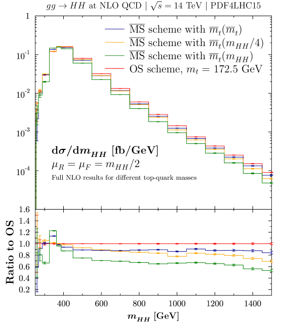
Figure 14: The differential Higgs-pair production cross section at NLO as a function of the invariant Higgs-pair mass for a c.m. energy of 14 TeV for four different choices of the scheme and scale of the top mass. The lower panel shows the ratio of all results to the default results with the top pole mass (OS scheme). PDF4LHC PDFs have been used and the renormalization and factorization scales of $\alpha_{s}$ and the PDFs have been fixed at our central scale choice $\mu_{R}=\mu_{F}=Q/2$.

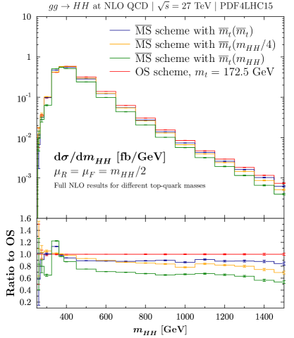
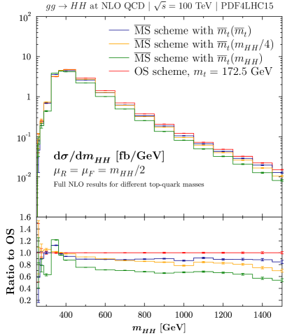
Figure 15: Same as Fig. 14 but for c.m. energies of 27 (left) and 100 (right) TeV.

It is clearly visible that the scale and scheme dependence of the top mass induces sizeable variations of the NLO Higgs-pair production cross section and thus contributes to the theoretical uncertainties. For small $Q$ values, the size pattern of the differential cross section due to the different scale and scheme choices is varying. For large values of $Q$, the maximum is always given by the on-shell scheme and the minimum in terms of the $\overline{\rm MS}$-top mass $\overline{m}_{t}(Q)$ with sizeable differences to the on-shell scheme. Adopting the related uncertainties as the envelope of the cross sections for our four choices, we arrive at the following uncertainties of the differential cross section for a c.m. energy $\sqrt{s}=14$ TeV,

$$\frac{d\sigma_{NLO}}{dQ}\Big{|}_{Q=300~{}{\rm GeV}} = 0.02978(7)^{+6\%}_{-34\%}\ {\rm fb/GeV},$$

$$\frac{d\sigma_{NLO}}{dQ}\Big{|}_{Q=400~{}{\rm GeV}} = 0.1609(4)^{+0\%}_{-13\%}\ {\rm fb/GeV},$$

$$\frac{d\sigma_{NLO}}{dQ}\Big{|}_{Q=600~{}{\rm GeV}} = 0.03204(9)^{+0\%}_{-30\%}\ {\rm fb/GeV},$$

$$\frac{d\sigma_{NLO}}{dQ}\Big{|}_{Q=1200~{}{\rm GeV}} = 0.000435(4)^{+0\%}_{-35\%}\ {\rm fb/GeV}\,.$$ (88)

Since these uncertainties are given relative to the on-shell results, the upper uncertainty vanishes for $Q\geq 400$ GeV, because the on-shell results provide the maximal values. These uncertainties turn out to be significant and at a similar level as the usual renormalization and factorization scale uncertainties. Thus, they constitute an additional contribution to the total theoretical uncertainties that has to be taken into account. The uncertainties due to the top-mass scheme and scale are about a factor of two smaller than at LO,

$$\frac{d\sigma_{LO}}{dQ}\Big{|}_{Q=300~{}{\rm GeV}} = 0.01656^{+62\%}_{-2.4\%}\,\mathrm{fb/GeV},$$

$$\frac{d\sigma_{LO}}{dQ}\Big{|}_{Q=400~{}{\rm GeV}} = 0.09391^{+0\%}_{-20\%}\,\mathrm{fb/GeV},$$

$$\frac{d\sigma_{LO}}{dQ}\Big{|}_{Q=600~{}{\rm GeV}} = 0.02132^{+0\%}_{-48\%}\,\mathrm{fb/GeV},$$

$$\frac{d\sigma_{LO}}{dQ}\Big{|}_{Q=1200~{}{\rm GeV}} = 0.0003223^{+0\%}_{-56\%}\,\mathrm{fb/GeV}$$ (89)

that have been obtained for a c.m. energy of 14 TeV and using PDF4LHC15 NLO parton densities with a NLO strong coupling normalized to $\alpha_{s}(M_{Z})=0.118$. Their reduction from LO to NLO underlines that the NLO QCD corrections stabilize the theoretical prediction for the Higgs-pair production cross section. The large size of the residual uncertainties is just a consequence of the large NLO QCD corrections as is the case for the renormalization and factorization scale dependences, too. Adopting the envelope for each $Q$-bin individually and integrating over $Q$, we arrive at the impact of these uncertainties on the total cross section for various c.m. energies,

$$\sqrt{s}=13~{}{\rm TeV}:\quad\sigma_{tot} = 27.73(7)^{+4\%}_{-18\%}~{}{\rm fb},$$

$$\sqrt{s}=14~{}{\rm TeV}:\quad\sigma_{tot} = 32.81(7)^{+4\%}_{-18\%}~{}{\rm fb},$$

$$\sqrt{s}=27~{}{\rm TeV}:\quad\sigma_{tot} = 127.0(2)^{+4\%}_{-18\%}~{}{\rm fb},$$

$$\sqrt{s}=100~{}{\rm TeV}:\quad\sigma_{tot} = 1140(2)^{+3\%}_{-18\%}~{}{\rm fb}$$ (90)

using PDF4LHC PDFs. A further reduction of these uncertainties can only be achieved by the determination or reliable estimate of the full mass effects at NNLO.

Since these uncertainties are sizeable, one may wonder why this has not been observed already for single-Higgs boson production $gg\to H$. The measured value of the Higgs mass $M_{H}=125$ GeV is small compared to the top mass so that for single on-shell Higgs production we are close to the HTL, i.e. finite top-mass effects are small and thus the related uncertainties, too. However, going to larger virtualities $Q$ for off-shell Higgs production $gg\to H^{*}$ (or larger Higgs masses for on-shell Higgs production), we arrive at similar uncertainties for $\sqrt{s}=14$ TeV,

$$\sigma_{NLO}\Big{|}_{Q=125~{}{\rm GeV}} =42.17^{+0.4\%}_{-0.5\%}\,\mathrm{pb},\qquad\sigma_{NLO}\Big{|}_{Q=300~{}{\rm GeV}} =9.85^{+7.5\%}_{-0.3\%}\,\mathrm{pb},$$

$$\sigma_{NLO}\Big{|}_{Q=400~{}{\rm GeV}} =9.43^{+0.1\%}_{-0.9\%}\,\mathrm{pb},\qquad\sigma_{NLO}\Big{|}_{Q=600~{}{\rm GeV}} =1.97^{+0.0\%}_{-15.9\%}\,\mathrm{pb},$$

$$\sigma_{NLO}\Big{|}_{Q=900~{}{\rm GeV}} =0.230^{+0.0\%}_{-22.3\%}\,\mathrm{pb},\quad\sigma_{NLO}\Big{|}_{Q=1200~{}{\rm GeV}} =0.0402^{+0.0\%}_{-26.0\%}\,\mathrm{pb}$$ (91)

using PDF4LHC PDFs. This has been known for a long time since there are sizeable effects on the virtual corrections due to the scale choice of the top mass for larger values of $Q$ or the Higgs mass (see Fig. 7a of Ref. Spira:1995rr ). For the single off-shell Higgs case, a reduction of the top-mass scale dependence by roughly a factor of two by going from LO to NLO has been observed, too, as can be inferred from the comparison with the explicit LO numbers for $\sqrt{s}=14$ TeV,

$$\sigma_{LO}\Big{|}_{Q=125~{}{\rm GeV}} =18.43^{+0.8\%}_{-1.1\%}\,\mathrm{pb},\qquad\sigma_{LO}\Big{|}_{Q=300~{}{\rm GeV}} =4.88^{+23.1\%}_{-1.1\%}\,\mathrm{pb},$$

$$\sigma_{LO}\Big{|}_{Q=400~{}{\rm GeV}} =4.94^{+1.2\%}_{-1.8\%}\,\mathrm{pb},\qquad\sigma_{LO}\Big{|}_{Q=600~{}{\rm GeV}} =1.13^{+0.0\%}_{-26.2\%}\,\mathrm{pb},$$

$$\sigma_{LO}\Big{|}_{Q=900~{}{\rm GeV}} =0.139^{+0.0\%}_{-36.0\%}\,\mathrm{pb},\quad\sigma_{LO}\Big{|}_{Q=1200~{}{\rm GeV}} =0.0249^{+0.0\%}_{-41.1\%}\,\mathrm{pb}$$ (92)

that have been obtained with PDF4LHC PDFs as in the Higgs-pair case. On the other hand, the uncertainties for $Q=125$ GeV confirm that they are small for on-shell Higgs production via gluon fusion (already at LO) in agreement with the analysis of the LHC Higgs Cross Section Working Group deFlorian:2016spz ; Anastasiou:2016cez .

A relevant issue is the theoretical background of the different scale choices for the top mass. For small values of $Q$, the matrix element will be closer to the HTL such that the NLO corrections get closer to the HTL calculation. The HTL on the other hand can be treated by starting from the effective Lagrangian of Eq. (21) which is the residual effective coupling of Higgs bosons to gluons after integrating out the top quark. Thus, the corresponding Wilson coefficients $C_{1}$ and $C_{2}$ are determined by matching the full SM with the top quark to the effective theory without the top quark. The matching scale is naturally given by the top mass. Performing the proper matching at the scale of the top mass, i.e. using either the top pole mass or the top $\overline{\rm MS}$ mass at the scale of the top mass itself leads to non-logarithmic (in the top mass) matching contributions [see Eq.(22) for $\mu_{R}=m_{t}$] also for higher powers in $1/m_{t}^{2}$, i.e. higher-dimensional operators contributing to the gluonic Higgs couplings at the subleading level. This implies that the top mass is the preferred scale choice for small values of $Q$. This is confirmed by the heavy top expansion of the form factors of Refs. Grigo:2013rya ; Grigo:2015dia ; Davies:2018qvx .

At large $Q$ values, on the other hand, we can use the results for the high-energy expansion of Ref. Davies:2018qvx . In the regime of large $Q$, the triangle-diagram contributions are suppressed by the $s$-channel Higgs propagator so that the box diagrams provide the dominant contributions. In our normalization, the explicit results of the virtual box-form factors in the high-energy limit ($Q\gg m_{t},M_{H}$) in terms of the top pole mass $m_{t}$ are given by

$$F_{i} = F_{i,LO}+\Delta F_{i}\,,$$

$$\Delta F_{i} = \Delta F_{i,HTL}+\Delta F_{i,mass}\,,$$

$$F_{1,LO} \to 4\frac{m_{t}^{2}}{\hat{s}}\,,$$

$$F_{2,LO} \to -\frac{m_{t}^{2}}{\hat{s}\hat{t}(\hat{s}+\hat{t})}\Big{\{}(\hat{s}+\hat{t})^{2}L_{1ts}^{2}+\hat{t}^{2}L_{ts}^{2}+\pi^{2}[(\hat{s}+\hat{t})^{2}+\hat{t}^{2}]\Big{\}}\,,$$

$$\Delta F_{1,mass} \to \frac{\alpha_{s}}{\pi}\left\{2F_{1,LO}\log\frac{m_{t}^{2}}{\hat{s}}+\frac{m_{t}^{2}}{\hat{s}}G_{1}(\hat{s},\hat{t})\right\}\,,$$

$$\Delta F_{2,mass} \to \frac{\alpha_{s}}{\pi}\left\{2F_{2,LO}\log\frac{m_{t}^{2}}{\hat{s}}+\frac{m_{t}^{2}}{\hat{s}}G_{2}(\hat{s},\hat{t})\right\}\,,$$ (93)

where $G_{1,2}(\hat{s},\hat{t})$ denote explicit and lengthy functions of the kinematical variables $\hat{s}$ and $\hat{t}$ that do not depend on the top mass Davies:2018qvx . The logarithms $L_{ts},L_{1ts}$ are defined as

$$L_{ts}=\log\left(-\frac{\hat{t}}{\hat{s}}\right)+i\pi\,,\qquad L_{1ts}=\log\left(1+\frac{\hat{t}}{\hat{s}}\right)+i\pi\,.$$ (94)

Transforming the top pole mass $m_{t}$ into the $\overline{\rm MS}$ mass $\overline{m}_{t}(\mu_{t})$, we arrive at the LO expressions for $F_{1/2,LO}$ with $m_{t}$ replaced by $\overline{m}_{t}(\mu_{t})$ and the appropriately transformed NLO coefficients

$$F_{1,LO} \to 4\frac{\overline{m}_{t}^{2}(\mu_{t})}{\hat{s}}\,,$$

$$F_{2,LO} \to -\frac{\overline{m}_{t}^{2}(\mu_{t})}{\hat{s}\hat{t}(\hat{s}+\hat{t})}\Big{\{}(\hat{s}+\hat{t})^{2}L_{1ts}^{2}+\hat{t}^{2}L_{ts}^{2}+\pi^{2}[(\hat{s}+\hat{t})^{2}+\hat{t}^{2}]\Big{\}}\,,$$

$$\Delta F_{1,mass} \to \frac{\alpha_{s}}{\pi}\left\{2F_{1,LO}\left[\log\frac{\mu_{t}^{2}}{\hat{s}}+\frac{4}{3}\right]+\frac{\overline{m}_{t}^{2}(\mu_{t})}{\hat{s}}G_{1}(\hat{s},\hat{t})\right\}\,,$$

$$\Delta F_{2,mass} \to \frac{\alpha_{s}}{\pi}\left\{2F_{2,LO}\left[\log\frac{\mu_{t}^{2}}{\hat{s}}+\frac{4}{3}\right]+\frac{\overline{m}_{t}^{2}(\mu_{t})}{\hat{s}}G_{2}(\hat{s},\hat{t})\right\}\,.$$ (95)

To minimize the logarithms of $\mu_{t}$, a dynamical scale of the order of $\sqrt{\hat{s}}=Q$ has to be chosen, but not the top mass. A coefficient $\kappa$ in front of the dynamical scale choice $\mu_{t}=\kappa Q$ is still arbitrary (but should not be large) since additional finite parts of the functions $G_{1,2}(\hat{s},\hat{t})$ may be absorbed in the scale choice. Thus, the dynamical scale $Q$ can be identified as the preferred central scale choice of the Yukawa couplings for large $Q$ values.

The uncertainties originating from the scheme and scale dependence of the top mass can be reduced by calculating the NNLO mass effects. Such a three-loop calculation is beyond everything that has been performed so far with current methods, but for $Q$ values close to threshold a large-mass expansion at NNLO could be used to reach an approximate estimate of the finite top-mass effects at NNLO. As a first step, partial results of the NNLO top-mass effects are known in the soft+virtual approximation Grigo:2015dia . For $Q$ values around the virtual $t\bar{t}$ threshold $Q\sim 2m_{t}$, non-relativistic Green’s functions could be used that allow the introduction of higher-order corrections to the QCD potential Fadin:1987wz ; Fadin:1988fn ; Fadin:1990wx ; Strassler:1990nw ; Melnikov:1994jb . This may lead to an improved description of the threshold region. However, for the triangle diagrams, the threshold behaviour is determined by $P$-wave contributions, since the $t\bar{t}$-ground state appears as a ${\cal CP}$-odd configuration that does not mix with the virtual ${\cal CP}$-even threshold state of the triangle diagrams. For the box diagrams, the $P$–wave contributions have to be considered, too. Moreover, it is unclear how large the impact of top-mass effects of the remainder beyond the non-relativistic Green’s functions will be. Finally, for the high-energy tail, the approximate calculation of Ref. Davies:2018qvx could be extended to NNLO.

4.4 Variation of the cross section with $\lambda_{H^{3}}$

Higgs-pair production at the LHC is directly sensitive to the trilinear Higgs coupling. The dependence of the total and differential cross sections on the trilinear coupling $\lambda_{H^{3}}$ is modified by the NLO QCD corrections and in particular by the finite mass effects at LO and NLO. Finite top-mass effects result in a non-vanishing matrix element at threshold, while in the HTL the matrix element of Eq. (4) vanishes exactly Glover:1987nx ; Plehn:1996wb ; Li:2013rra ,

$${\cal A}^{\mu\nu} \to F_{1}T_{1}^{\mu\nu}\,,$$

$$F_{1} \to \frac{2}{3}(C_{\triangle}-1)\to\frac{2}{3}~{}\left(\frac{3M_{H}^{2}}{4M_{H}^{2}-M_{H}^{2}}-1\right)=0\qquad\mbox{for $Q^{2}\to(2M_{H})^{2}$}\,,$$ (96)

where we have used that the second form factor $G_{\Box}$ vanishes in the HTL [see Eq. (9)]. The cancellation is induced by the destructive interference between the triangle and box diagrams at LO. This property is modified by finite subleading ${\cal O}(1/m_{t}^{2})$ terms but explains why the matrix element itself is suppressed at the production threshold. As a function of $\lambda_{H^{3}}$, the cross section develops a minimum at $\lambda_{H^{3}}$-values around 2.4 times the SM-value in the Born-improved HTL Dawson:1998py ; Baglio:2012np since the phase-space integration adds contributions from above the production threshold. The NLO QCD corrections will shift the minimum of the cross section as a function of $\lambda_{H^{3}}$ and finite top-mass effects play a prominent role in the amount of these cancellations. For the determination of the trilinear coupling, the variation of the cross section with $\lambda_{H^{3}}$ is of interest. As mentioned in the introduction, the total cross section behaves approximately as $\Delta\sigma/\sigma\sim-\Delta\lambda_{H^{3}}/\lambda_{H^{3}}$ for $\lambda_{H^{3}}$ close to the SM value.

In the following, we will analyze the NLO results, where only the trilinear coupling has been varied. In general, however, several coupling modifications contribute to the Higgs-pair production cross section. This could be treated consistently by extending the SM Lagrangian by all contributing dimension-6 operators as has been studied in Ref. Grober:2015cwa in the HTL at NLO and in Ref. deFlorian:2017qfk at NNLO. Recently the HTL analysis has been extended to the inclusion of finite top-mass effects at NLO Buchalla:2018yce . However, we will neglect all dimension-6 operators but the one modifying the Higgs self-interactions. A proper and consistent effective model of this type has been discussed in Ref. Degrassi:2017ucl that adds higher-dimension operators to the scalar Higgs sector only. Thus, a sole variation of the Higgs self-interactions could be realized within Higgs portal models with additional heavy scalar states that couple only to the SM-like Higgs field and are integrated out.

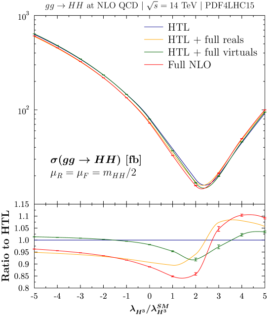
Figure 16: The total Higgs-pair production cross section at NLO as a function of the trilinear self-coupling $\lambda_{H^{3}}$ in units of the SM value for a c.m. energy of 14 TeV. The blue curve shows the Born-improved HTL, the yellow includes the NLO mass effects of the real corrections in addition and the green curve those of the virtual corrections in addition. The full NLO result is presented by the red curve. The lower panel shows the ratio of all results to the Born-improved HTL. PDF4LHC PDFs have been used and the renormalization and factorization scales of $\alpha_{s}$ and the PDFs have been fixed at our central scale choice $\mu_{R}=\mu_{F}=Q/2=m_{HH}/2$.

In Figs. 16 and 17, the dependence of the total Higgs-pair production cross section is shown as a function of the trilinear Higgs coupling $\lambda_{H^{3}}$ in units of the SM coupling for three c.m. energies, 14, 27 and 100 TeV. The blue curves display the results in the Born-improved HTL, the yellow curves include the mass effects of the real corrections and the green curves the mass effects of virtual corrections in addition. The red curves exhibit the complete NLO results. The comparison of the blue and red curves indicates that the minimum of the $\lambda_{H^{3}}$-variation is shifted from about 2.4 times the SM value to about 2.3 times the SM value due to the NLO mass effects. The yellow and green curves imply that the main origin of this shift emerges from the mass effects of the real corrections. The lower panels of Figs. 16 and 17 present the ratios of the individual contributions to the Born-improved HTL. While the NLO mass effects are of moderate size for negative values of $\lambda_{H^{3}}$, where the triangle and box diagrams interfere constructively, they turn out to be more relevant in the region of destructive interference, in particular around the minima of the cross sections. The significantly varying NLO mass effects have to be taken into account when determining the value of $\lambda_{H^{3}}$ from the experimental data at the HL-LHC. This agrees with the findings of Ref. Buchalla:2018yce . The NLO mass effects on the variation of the total cross section with $\lambda_{H^{3}}$ become larger with rising c.m. energy of the hadron collider.

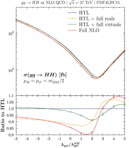
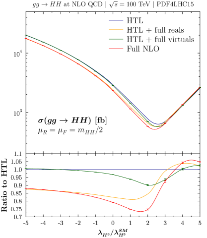
Figure 17: Same as Fig. 16 but for c.m. energies of 27 (left) and 100 (right) TeV.

In Fig. 18, we display the consistently defined K-factors $K=\sigma_{NLO}/\sigma_{LO}$ as a function of $\lambda_{H^{3}}$ in units of the SM coupling. The full curves show the NLO K-factors including the NLO top-mass effects for various c.m. energies. The dotted curves exhibit the corresponding K-factors in the Born-improved HTL as computed in Refs. Dawson:1998py ; Grober:2015cwa . The impact of the NLO mass effects on the K-factors ranges at the level of 10–15% for negative $\lambda_{H^{3}}$ values, where the triangle and box diagrams interfere constructively. For positive values of $\lambda_{H^{3}}$ (destructive interference), the size and sign of the NLO mass effects is changing considerably as can be inferred from the comparison to the dotted curves. The full K-factors develop a larger dependence on $\lambda_{H^{3}}$ than the Born-improved HTL due to the NLO top-mass effects. This confirms the findings of Ref. Buchalla:2018yce . The NLO top-mass effects of the total cross section increase with rising collider energy in general except for the regions of destructive interference between the triangle and box diagrams (positive $\lambda_{H^{3}}$).

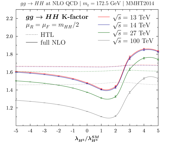
Figure 18: K-factors of Higgs-pair production at NLO as functions of the trilinear self-coupling $\lambda_{H^{3}}$ in units of the SM value $\lambda_{H^{3}}^{SM}$ for various c.m. energies of 13 TeV (red curves), 14 TeV (blue curves), 27 TeV (green curves) and 100 TeV (grey curves). The full NLO result is presented by the full curves with the error bars indicating our numerical errors. The dotted curves show the corresponding K-factors of the Born-improved HTL. MMHT2014 PDFs have been used and the renormalization and factorization scales of $\alpha_{s}$ and the PDFs have been fixed at our central scale choice $\mu_{R}=\mu_{F}=Q/2=m_{HH}/2$.

The full NLO cross section as a function of $\lambda_{H^{3}}$ can be parametrized as

$$\sigma_{NLO}=\sigma_{1}+\sigma_{2}\frac{\lambda_{H^{3}}}{\lambda^{SM}_{H^{3}}}+\sigma_{3}\left(\frac{\lambda_{H^{3}}}{\lambda^{SM}_{H^{3}}}\right)^{2}\,.$$ (97)

The coefficients $\sigma_{1\ldots 3}$ depend on the c.m. energy of the hadron collider and on the PDFs used in their evaluation. For the various c.m. energies, we obtain the following NLO values for PDF4LHC PDFs and our central scale choices $\mu_{R}=\mu_{F}=Q/2$,

$$\sqrt{s}=13~{}{\rm TeV}:\quad\sigma_{1} = 61.35(6)~{}{\rm fb}\,,\quad\sigma_{2}=-43.26(5)~{}{\rm fb}\,,\quad\sigma_{3}=9.62(8)~{}{\rm fb}\,,$$

$$\sqrt{s}=14~{}{\rm TeV}:\quad\sigma_{1} = 72.27(7)~{}{\rm fb}\,,\quad\sigma_{2}=-50.70(6)~{}{\rm fb}\,,\quad\sigma_{3}=11.23(9)~{}{\rm fb}\,,$$

$$\sqrt{s}=27~{}{\rm TeV}:\quad\sigma_{1} = 270.9(3)~{}{\rm fb}\,,\quad\sigma_{2}=-183.1(2)~{}{\rm fb}\,,\quad\sigma_{3}=39.5(4)~{}{\rm fb}\,,$$

$$\sqrt{s}=100~{}{\rm TeV}:\quad\sigma_{1} = 2323(2)~{}{\rm fb}\,,\quad\;\sigma_{2}=-1496(2)~{}{\rm fb}\,,\quad\;\sigma_{3}=313(3)~{}{\rm fb}\,,$$ (98)

where the numbers in brackets denote our numerical errors. The corresponding coefficients with MMHT2014 PDFs read

$$\sqrt{s}=13~{}{\rm TeV}:\quad\sigma_{1} = 62.45(7)~{}{\rm fb}\,,\quad\sigma_{2}=-44.13(5)~{}{\rm fb}\,,\quad\sigma_{3}=9.83(9)~{}{\rm fb}\,,$$

$$\sqrt{s}=14~{}{\rm TeV}:\quad\sigma_{1} = 73.60(8)~{}{\rm fb}\,,\quad\sigma_{2}=-51.75(6)~{}{\rm fb}\,,\quad\sigma_{3}=11.5(1)~{}{\rm fb}\,,$$

$$\sqrt{s}=27~{}{\rm TeV}:\quad\sigma_{1} = 277.4(3)~{}{\rm fb}\,,\quad\sigma_{2}=-187.9(2)~{}{\rm fb}\,,\quad\sigma_{3}=40.6(4)~{}{\rm fb}\,,$$

$$\sqrt{s}=100~{}{\rm TeV}:\quad\sigma_{1} = 2401(2)~{}{\rm fb}\,,\quad\;\sigma_{2}=-1550(2)~{}{\rm fb}\,,\quad\;\sigma_{3}=325(3)~{}{\rm fb}\,.$$ (99)

It should be noted that the final numerical errors of the cross sections as shown in Figs. 16–18 are smaller than the ones emerging from using the coefficients of Eqs. (98, 99) since the combinations of each bin in $Q$ before integration reduces them.

5 Conclusions

In this work, we have discussed the full QCD corrections to Higgs-pair production at NLO. We have explained the details of our numerical approach to solve the multi-scale two-loop integrals involving ultraviolet and infrared singularities. The ultraviolet singularities could be extracted from the finite parts by suitable end-point subtractions, while the infrared singularities have been isolated by means of dedicated subtraction terms. The ultraviolet singularities have been absorbed by the proper renormalization of the strong coupling and the top mass, while the infrared ones cancel against the one-loop real corrections involving an additional gluon or quark in the final state of the Higgs-boson pair. We have performed the evaluation of the virtual corrections diagram by diagram without tensor reduction.

The emerging integrals develop thresholds if the virtual $t\bar{t}$-threshold is crossed, but also at small virtualities due to the presence of purely gluonic intermediate states. The numerical stabilization of the virtual two-loop integrals has been achieved through integrations by parts of the integrands such that the power of the threshold-singular denominators is reduced. The narrow-width limit of the virtual top quarks has been obtained by a Richardson extrapolation of the results for different sizes of an auxiliarly introduced width parameter. This has allowed a numerical integration of the virtual two-loop corrections with an accuracy of less than one per cent.

The matrix elements for the real corrections have been generated with FeynArts and FormCalc and integrated using the library Collier. The collinear region of the phase-space integration has been regularized numerically by a technical cut.

We have subtracted the Born-improved HTL from the virtual and real corrections individually so that we have been left with the pure NLO top-mass effects beyond the Born-improved HTL that is implemented in the public tool Hpair. Thus, the final NLO results have been obtained by adding back the numbers from Hpair.

The final results have been analyzed in detail for the differential cross section in the invariant Higgs-pair mass and the total cross section. Finite top-mass effects beyond the Born-improved HTL decrease the total cross section by about 15% at the LHC. However, the negative mass effects are larger for the differential cross section reaching a level of $-30\%$ or $-40\%$ for large invariant Higgs-pair masses. This implies that the inclusion of the NLO top-mass effects is crucial for a reliable analysis at the LHC and future proton colliders. We have discussed the usual renormalization and factorization scale uncertainties that are in agreement with previous calculations. However, we have identified an additional scale and scheme uncertainty due to the virtual top mass. This uncertainty reaches a level of 15% for the total cross section but can be larger (up to 35%) for the differential cross section. Based on the heavy-top and high-energy expansions, we have discussed the preferred scale choices of the running top mass and identified a large dynamical scale as the proper choice for large invariant Higgs-pair masses. This additional uncertainty has to be combined with the usual renormalization and factorization scale uncertainties. Since the (relative) scheme and scale uncertainties originating from the top mass only mildly depend on the renormalization and factorization scale choice, the addition of this uncertainty may lead to about a linear addition to the other uncertainties, if the total uncertainty is defined as the envelope. This, however, has to be analyzed in more detail which is left for future work.

We have investigated the total cross section as a function of the trilinear coupling varied from its SM value. We have found significant NLO mass effects beyond the Born-improved HTL that result in a shift of the minimum of the cross section at various present and future c.m. energies of the hadron colliders. While the main effect of shifting the minimum originates from the NLO top-mass effects of the real corrections, the more symmetric virtual mass effects mainly affect the size of the total cross section as a function of $\lambda_{H^{3}}$. The full K-factors develop a larger dependence on $\lambda_{H^{3}}$ than those of the Born-improved HTL due to the NLO top-mass effects.

Acknowledgements
We are indebted to S. Dittmaier for providing us with a copy of his mathematica program for the QCD corrections in the HTL as constructed for the work of Ref. Dawson:1998py and to R. Gröber for useful discussions. The work of S. G. is supported by the Swiss National Science Foundation (SNF). The work of S. G. and M. M. is supported by the DFG Collaborative Research Center TRR 257 “Particle Physics Phenomenology after the Higgs Discovery”. F. C. and J. R. acknowledge financial support by the Generalitat Valenciana, Spanish Government and ERDF funds from the European Commission (Grants No. RYC-2014-16061, SEJI-2017/2017/019, FPA2017-84543- P,FPA2017-84445-P, and SEV-2014-0398). We acknowledge support by the state of Baden-Württemberg through bwHPC and the German Research Foundation (DFG) through grant no INST 39/963-1 FUGG (bwForCluster NEMO).

Appendix A Two-loop box diagrams of the virtual corrections

Here we present the two-loop box diagrams (omitting the ones with reversed fermion flow):

Figure 19: Two-loop box diagrams: topologies 1 and 2.

Figure 20: Two-loop box diagrams: topologies 3 and 4.

Figure 21: Two-loop box diagrams: topologies 5 and 6.

References

- (1) ATLAS collaboration, Observation of a new particle in the search for the Standard Model Higgs boson with the ATLAS detector at the LHC, Phys. Lett. B716 (2012) 1 [1207.7214].
- (2) CMS collaboration, Observation of a new boson at a mass of 125 GeV with the CMS experiment at the LHC, Phys. Lett. B716 (2012) 30 [1207.7235].
- (3) ATLAS, CMS collaboration, Measurements of the Higgs boson production and decay rates and constraints on its couplings from a combined ATLAS and CMS analysis of the LHC pp collision data at and 8 TeV, JHEP 08 (2016) 045 [1606.02266].
- (4) P. W. Higgs, Broken symmetries, massless particles and gauge fields, Phys. Lett. 12 (1964) 132.
- (5) P. W. Higgs, Broken Symmetries and the Masses of Gauge Bosons, Phys. Rev. Lett. 13 (1964) 508.
- (6) P. W. Higgs, Spontaneous Symmetry Breakdown without Massless Bosons, Phys. Rev. 145 (1966) 1156.
- (7) F. Englert and R. Brout, Broken Symmetry and the Mass of Gauge Vector Mesons, Phys. Rev. Lett. 13 (1964) 321.
- (8) G. S. Guralnik, C. R. Hagen and T. W. B. Kibble, Global Conservation Laws and Massless Particles, Phys. Rev. Lett. 13 (1964) 585.
- (9) T. W. B. Kibble, Symmetry breaking in nonAbelian gauge theories, Phys. Rev. 155 (1967) 1554.
- (10) E. N. Glover and J. van der Bij, Higgs boson pair production via gluon fusion, Nucl. Phys. B309 (1988) 282.
- (11) T. Plehn, M. Spira and P. M. Zerwas, Pair production of neutral Higgs particles in gluon-gluon collisions, Nucl. Phys. B479 (1996) 46 [hep-ph/9603205]. [Erratum: Nucl. Phys. B531 (1998) 655].
- (12) S. Dawson, S. Dittmaier and M. Spira, Neutral Higgs boson pair production at hadron colliders: QCD corrections, Phys. Rev. D58 (1998) 115012 [hep-ph/9805244].
- (13) A. Djouadi, W. Kilian, M. Mühlleitner and P. M. Zerwas, Production of neutral Higgs boson pairs at LHC, Eur. Phys. J. C10 (1999) 45 [hep-ph/9904287].
- (14) J. Baglio, A. Djouadi, R. Gröber, M. M. Mühlleitner, J. Quevillon and M. Spira, The measurement of the Higgs self-coupling at the LHC: theoretical status, JHEP 04 (2013) 151 [1212.5581].
- (15) G. Degrassi, P. P. Giardino, F. Maltoni and D. Pagani, Probing the Higgs self coupling via single Higgs production at the LHC, JHEP 12 (2016) 080 [1607.04251].
- (16) G. Degrassi, M. Fedele and P. P. Giardino, Constraints on the trilinear Higgs self coupling from precision observables, JHEP 04 (2017) 155 [1702.01737].
- (17) T. Plehn and M. Rauch, The quartic higgs coupling at hadron colliders, Phys. Rev. D72 (2005) 053008 [hep-ph/0507321].
- (18) T. Binoth, S. Karg, N. Kauer and R. Rückl, Multi-Higgs boson production in the Standard Model and beyond, Phys. Rev. D74 (2006) 113008 [hep-ph/0608057].
- (19) B. Fuks, J. H. Kim and S. J. Lee, Probing Higgs self-interactions in proton-proton collisions at a center-of-mass energy of 100 TeV, Phys. Rev. D93 (2016) 035026 [1510.07697].
- (20) D. de Florian and J. Mazzitelli, Two-loop corrections to the triple Higgs boson production cross section, JHEP 02 (2017) 107 [1610.05012].
- (21) D. de Florian, J. Mazzitelli and I. Fabre, Triple Higgs production at hadron colliders at NNLO in QCD, 1912.02760.
- (22) T. Liu, K.-F. Lyu, J. Ren and H. X. Zhu, Probing the quartic Higgs boson self-interaction, Phys. Rev. D98 (2018) 093004 [1803.04359].
- (23) W. Bizoń, U. Haisch and L. Rottoli, Constraints on the quartic Higgs self-coupling from double-Higgs production at future hadron colliders, JHEP 10 (2019) 267 [1810.04665].
- (24) S. Borowka, C. Duhr, F. Maltoni, D. Pagani, A. Shivaji and X. Zhao, Probing the scalar potential via double Higgs boson production at hadron colliders, JHEP 04 (2019) 016 [1811.12366].
- (25) S. Borowka, N. Greiner, G. Heinrich, S. Jones, M. Kerner, J. Schlenk et al., Higgs Boson Pair Production in Gluon Fusion at Next-to-Leading Order with Full Top-Quark Mass Dependence, Phys. Rev. Lett. 117 (2016) 012001 [1604.06447]. [Erratum: Phys. Rev. Lett. 117 (2016) 079901].
- (26) S. Borowka, N. Greiner, G. Heinrich, S. P. Jones, M. Kerner, J. Schlenk et al., Full top quark mass dependence in Higgs boson pair production at NLO, JHEP 10 (2016) 107 [1608.04798].
- (27) J. Baglio, F. Campanario, S. Glaus, M. Mühlleitner, M. Spira and J. Streicher, Gluon fusion into Higgs pairs at NLO QCD and the top mass scheme, Eur. Phys. J. C79 (2019) 459 [1811.05692].
- (28) D. de Florian and J. Mazzitelli, Two-loop virtual corrections to Higgs pair production, Phys. Lett. B724 (2013) 306 [1305.5206].
- (29) D. de Florian and J. Mazzitelli, Higgs Boson Pair Production at Next-to-Next-to-Leading Order in QCD, Phys. Rev. Lett. 111 (2013) 201801 [1309.6594].
- (30) J. Grigo, K. Melnikov and M. Steinhauser, Virtual corrections to Higgs boson pair production in the large top quark mass limit, Nucl. Phys. B888 (2014) 17 [1408.2422].
- (31) P. Banerjee, S. Borowka, P. K. Dhani, T. Gehrmann and V. Ravindran, Two-loop massless QCD corrections to the four-point amplitude, JHEP 11 (2018) 130 [1809.05388].
- (32) L.-B. Chen, H. T. Li, H.-S. Shao and J. Wang, Higgs boson pair production via gluon fusion at N3LO in QCD, 1909.06808.
- (33) L.-B. Chen, H. T. Li, H.-S. Shao and J. Wang, The gluon-fusion production of Higgs boson pair: N3LO QCD corrections and top-quark mass effects, JHEP 03 (2020) 072 [1912.13001].
- (34) M. Spira, Effective Multi-Higgs Couplings to Gluons, JHEP 10 (2016) 026 [1607.05548].
- (35) G. Heinrich, S. P. Jones, M. Kerner, G. Luisoni and E. Vryonidou, NLO predictions for Higgs boson pair production with full top quark mass dependence matched to parton showers, JHEP 08 (2017) 088 [1703.09252].
- (36) S. Jones and S. Kuttimalai, Parton Shower and NLO-Matching uncertainties in Higgs Boson Pair Production, JHEP 02 (2018) 176 [1711.03319].
- (37) M. Grazzini, G. Heinrich, S. Jones, S. Kallweit, M. Kerner, J. M. Lindert et al., Higgs boson pair production at NNLO with top quark mass effects, JHEP 05 (2018) 059 [1803.02463].
- (38) FCC collaboration, HE-LHC: The High-Energy Large Hadron Collider, Eur. Phys. J. ST 228 (2019) 1109.
- (39) FCC collaboration, FCC Physics Opportunities, Eur. Phys. J. C79 (2019) 474.
- (40) FCC collaboration, FCC-hh: The Hadron Collider, Eur. Phys. J. ST 228 (2019) 755.
- (41) D. Graudenz, M. Spira and P. M. Zerwas, QCD corrections to Higgs boson production at proton proton colliders, Phys. Rev. Lett. 70 (1993) 1372.
- (42) M. Spira, A. Djouadi, D. Graudenz and P. M. Zerwas, Higgs boson production at the LHC, Nucl. Phys. B453 (1995) 17 [hep-ph/9504378].
- (43) R. Harlander and P. Kant, Higgs production and decay: Analytic results at next-to-leading order QCD, JHEP 12 (2005) 015 [hep-ph/0509189].
- (44) C. Anastasiou, S. Bucherer and Z. Kunszt, HPro: A NLO Monte-Carlo for Higgs production via gluon fusion with finite heavy quark masses, JHEP 10 (2009) 068 [0907.2362].
- (45) U. Aglietti, R. Bonciani, G. Degrassi and A. Vicini, Analytic Results for Virtual QCD Corrections to Higgs Production and Decay, JHEP 01 (2007) 021 [hep-ph/0611266].
- (46) G. Altarelli and G. Parisi, Asymptotic Freedom in Parton Language, Nucl. Phys. B126 (1977) 298.
- (47) J. R. Ellis, M. K. Gaillard and D. V. Nanopoulos, A Phenomenological Profile of the Higgs Boson, Nucl. Phys. B106 (1976) 292.
- (48) M. A. Shifman, A. I. Vainshtein, M. B. Voloshin and V. I. Zakharov, Low-Energy Theorems for Higgs Boson Couplings to Photons, Sov. J. Nucl. Phys. 30 (1979) 711. [Yad. Fiz.30,1368(1979)].
- (49) T. Inami, T. Kubota and Y. Okada, Effective Gauge Theory and the Effect of Heavy Quarks in Higgs Boson Decays, Z. Phys. C18 (1983) 69.
- (50) B. A. Kniehl and M. Spira, Low-energy theorems in Higgs physics, Z. Phys. C69 (1995) 77 [hep-ph/9505225].
- (51) K. G. Chetyrkin, B. A. Kniehl and M. Steinhauser, Hadronic Higgs decay to order , Phys. Rev. Lett. 79 (1997) 353 [hep-ph/9705240].
- (52) M. Krämer, E. Laenen and M. Spira, Soft gluon radiation in Higgs boson production at the LHC, Nucl. Phys. B511 (1998) 523 [hep-ph/9611272].
- (53) Y. Schröder and M. Steinhauser, Four-loop decoupling relations for the strong coupling, JHEP 01 (2006) 051 [hep-ph/0512058].
- (54) P. A. Baikov, K. G. Chetyrkin and J. H. Kühn, Five-Loop Running of the QCD coupling constant, Phys. Rev. Lett. 118 (2017) 082002 [1606.08659].
- (55) M. Gerlach, F. Herren and M. Steinhauser, Wilson coefficients for Higgs boson production and decoupling relations to , JHEP 11 (2018) 141 [1809.06787].
- (56) D. Y. Shao, C. S. Li, H. T. Li and J. Wang, Threshold resummation effects in Higgs boson pair production at the LHC, JHEP 07 (2013) 169 [1301.1245].
- (57) D. de Florian and J. Mazzitelli, Higgs pair production at next-to-next-to-leading logarithmic accuracy at the LHC, JHEP 09 (2015) 053 [1505.07122].
- (58) R. Frederix, S. Frixione, V. Hirschi, F. Maltoni, O. Mattelaer et al., Higgs pair production at the LHC with NLO and parton-shower effects, Phys. Lett. B732 (2014) 142 [1401.7340].
- (59) F. Maltoni, E. Vryonidou and M. Zaro, Top-quark mass effects in double and triple Higgs production in gluon-gluon fusion at NLO, JHEP 1411 (2014) 079 [1408.6542].
- (60) J. Alwall, R. Frederix, S. Frixione, V. Hirschi, F. Maltoni et al., The automated computation of tree-level and next-to-leading order differential cross sections, and their matching to parton shower simulations, JHEP 1407 (2014) 079 [1405.0301].
- (61) V. Hirschi and O. Mattelaer, Automated event generation for loop-induced processes, JHEP 10 (2015) 146 [1507.00020].
- (62) J. Grigo, J. Hoff, K. Melnikov and M. Steinhauser, On the Higgs boson pair production at the LHC, Nucl. Phys. B875 (2013) 1 [1305.7340].
- (63) J. Grigo, J. Hoff and M. Steinhauser, Higgs boson pair production: top quark mass effects at NLO and NNLO, Nucl. Phys. B900 (2015) 412 [1508.00909].
- (64) R. Gröber, A. Maier and T. Rauh, Reconstruction of top-quark mass effects in Higgs pair production and other gluon-fusion processes, JHEP 03 (2018) 020 [1709.07799].
- (65) R. Bonciani, G. Degrassi, P. P. Giardino and R. Gröber, Analytical Method for Next-to-Leading-Order QCD Corrections to Double-Higgs Production, Phys. Rev. Lett. 121 (2018) 162003 [1806.11564].
- (66) J. Davies, G. Mishima, M. Steinhauser and D. Wellmann, Double Higgs boson production at NLO in the high-energy limit: complete analytic results, JHEP 01 (2019) 176 [1811.05489].
- (67) J. Davies, G. Heinrich, S. P. Jones, M. Kerner, G. Mishima, M. Steinhauser et al., Double Higgs boson production at NLO: combining the exact numerical result and high-energy expansion, JHEP 11 (2019) 024 [1907.06408].
- (68) The program Hpair can be obtained at the URL: http://tiger.web.psi.ch/hpair/ .
- (69) R. N. Cahn, M. S. Chanowitz and N. Fleishon, Higgs Particle Production by , Phys. Lett. 82B (1979) 113.
- (70) L. Bergström and G. Hulth, Induced Higgs Couplings to Neutral Bosons in Collisions, Nucl. Phys. B259 (1985) 137. [Erratum: Nucl. Phys.B276,744(1986)].
- (71) J. F. Gunion, H. E. Haber, G. L. Kane and S. Dawson, The Higgs Hunter’s Guide, Front. Phys. 80 (2000) 1.
- (72) G. Degrassi, P. P. Giardino and R. Gröber, On the two-loop virtual QCD corrections to Higgs boson pair production in the Standard Model, Eur. Phys. J. C76 (2016) 411 [1603.00385].
- (73) D. de Florian, I. Fabre and J. Mazzitelli, Higgs boson pair production at NNLO in QCD including dimension 6 operators, JHEP 10 (2017) 215 [1704.05700].
- (74) J. A. M. Vermaseren, New features of FORM, math-ph/0010025.
- (75) J. Kuipers, T. Ueda, J. A. M. Vermaseren and J. Vollinga, FORM version 4.0, Comput. Phys. Commun. 184 (2013) 1453 [1203.6543].
- (76) A. C. Hearn, Reduce 2: A System and Language For Algebraic Manipulation, PRINT-71-1192 (1971) .
- (77) Wolfram Research, Inc., Mathematica, Version 9.0, Champaign, IL (2012) .
- (78) A. Djouadi, M. Spira, J. J. van der Bij and P. M. Zerwas, QCD corrections to gamma gamma decays of Higgs particles in the intermediate mass range, Phys. Lett. B257 (1991) 187.
- (79) M. Spira, A. Djouadi and P. M. Zerwas, QCD corrections to the H Z gamma coupling, Phys. Lett. B276 (1992) 350.
- (80) M. Mühlleitner and M. Spira, Higgs Boson Production via Gluon Fusion: Squark Loops at NLO QCD, Nucl. Phys. B790 (2008) 1 [hep-ph/0612254].
- (81) M. Spira, Radiative QCD corrections to decay and production of Higgs bosons at and accelerators. (In German), Ph.D. thesis, Aachen, Tech. Hochsch., 1993.
- (82) M. Mühlleitner, H. Rzehak and M. Spira, SUSY-QCD Corrections to MSSM Higgs Boson Production via Gluon fusion, PoS RADCOR2009 (2010) 043 [1001.3214].
- (83) M. Mühlleitner, H. Rzehak and M. Spira, MSSM Higgs boson production via gluon fusion, in Physics at the LHC2010. Proceedings, 5th Conference, PLHC2010, Hamburg, Germany, June 7-12, 2010, pp. 415–417, 2010, DOI.
- (84) L. F. Richardson, The approximate arithmetical solution by finite differences of physical problems including differential equations, with an application to the stresses in a masonry dam, Philosophical Transactions of the Royal Society A210 (1911) 307.
- (85) N. Gray, D. J. Broadhurst, W. Grafe and K. Schilcher, Three Loop Relation of Quark (Modified) Ms and Pole Masses, Z. Phys. C48 (1990) 673.
- (86) K. G. Chetyrkin and M. Steinhauser, Short distance mass of a heavy quark at order , Phys. Rev. Lett. 83 (1999) 4001 [hep-ph/9907509].
- (87) K. G. Chetyrkin and M. Steinhauser, The Relation between the MS-bar and the on-shell quark mass at order , Nucl. Phys. B573 (2000) 617 [hep-ph/9911434].
- (88) K. Melnikov and T. v. Ritbergen, The Three loop relation between the MS-bar and the pole quark masses, Phys. Lett. B482 (2000) 99 [hep-ph/9912391].
- (89) O. V. Tarasov, Anomalous Dimensions of Quark Masses in three Loop Approximation, JINR-P2-82-900 (1982) .
- (90) K. G. Chetyrkin, Quark mass anomalous dimension to O(), Phys. Lett. B404 (1997) 161 [hep-ph/9703278].
- (91) G. P. Lepage, Vegas: An adaptive multidimensional Integration Program, CLNS-80/447 (1980) .
- (92) S. Catani and M. H. Seymour, A General algorithm for calculating jet cross-sections in NLO QCD, Nucl. Phys. B485 (1997) 291 [hep-ph/9605323]. [Erratum: Nucl. Phys.B510,503(1998)].
- (93) T. Hahn, Generating Feynman diagrams and amplitudes with FeynArts 3, Comput. Phys. Commun. 140 (2001) 418 [hep-ph/0012260].
- (94) T. Hahn and M. Perez-Victoria, Automatized one loop calculations in four-dimensions and D-dimensions, Comput. Phys. Commun. 118 (1999) 153 [hep-ph/9807565].
- (95) G. ’t Hooft and M. J. G. Veltman, Scalar One Loop Integrals, Nucl. Phys. B153 (1979) 365.
- (96) G. J. van Oldenborgh, FF: A Package to evaluate one loop Feynman diagrams, Comput. Phys. Commun. 66 (1991) 1.
- (97) A. Denner and S. Dittmaier, Reduction of one loop tensor five point integrals, Nucl. Phys. B658 (2003) 175 [hep-ph/0212259].
- (98) A. Denner and S. Dittmaier, Reduction schemes for one-loop tensor integrals, Nucl. Phys. B734 (2006) 62 [hep-ph/0509141].
- (99) A. Denner and S. Dittmaier, Scalar one-loop 4-point integrals, Nucl. Phys. B844 (2011) 199 [1005.2076].
- (100) A. Denner, S. Dittmaier and L. Hofer, Collier: a fortran-based Complex One-Loop LIbrary in Extended Regularizations, Comput. Phys. Commun. 212 (2017) 220 [1604.06792].
- (101) L. A. Harland-Lang, A. D. Martin, P. Motylinski and R. S. Thorne, Parton distributions in the LHC era: MMHT 2014 PDFs, Eur. Phys. J. C75 (2015) 204 [1412.3989].
- (102) J. Butterworth et al., PDF4LHC recommendations for LHC Run II, J. Phys. G43 (2016) 023001 [1510.03865].
- (103) A. Buckley, J. Ferrando, S. Lloyd, K. Nordström, B. Page, M. Rüfenacht et al., LHAPDF6: parton density access in the LHC precision era, Eur. Phys. J. C75 (2015) 132 [1412.7420].
- (104) M. Abramowitz and I. Stegun, Handbook of Mathematical Functions with Formulas, Graphs, and Mathematical Tables, Applied Mathematics Series 55 (1964) 307.
- (105) LHC Higgs Cross Section Working Group collaboration, Handbook of LHC Higgs Cross Sections: 4. Deciphering the Nature of the Higgs Sector, 1610.07922.
- (106) C. Anastasiou, C. Duhr, F. Dulat, E. Furlan, T. Gehrmann, F. Herzog et al., High precision determination of the gluon fusion Higgs boson cross-section at the LHC, JHEP 05 (2016) 058 [1602.00695].
- (107) V. S. Fadin and V. A. Khoze, Threshold Behavior of Heavy Top Production in Collisions, JETP Lett. 46 (1987) 525. [Pisma Zh. Eksp. Teor. Fiz.46,417(1987)].
- (108) V. S. Fadin and V. A. Khoze, Production of a pair of heavy quarks in annihilation in the threshold region, Sov. J. Nucl. Phys. 48 (1988) 309. [Yad. Fiz.48,487(1988)].
- (109) V. S. Fadin, V. A. Khoze and T. Sjostrand, On the Threshold Behavior of Heavy Top Production, Z. Phys. C48 (1990) 613.
- (110) M. J. Strassler and M. E. Peskin, The Heavy top quark threshold: QCD and the Higgs, Phys. Rev. D43 (1991) 1500.
- (111) K. Melnikov, M. Spira and O. I. Yakovlev, Threshold effects in two photon decays of Higgs particles, Z. Phys. C64 (1994) 401 [hep-ph/9405301].
- (112) X. Li and M. B. Voloshin, Remarks on double Higgs boson production by gluon fusion at threshold, Phys. Rev. D89 (2014) 013012 [1311.5156].
- (113) R. Gröber, M. Mühlleitner, M. Spira and J. Streicher, NLO QCD Corrections to Higgs Pair Production including Dimension-6 Operators, JHEP 09 (2015) 092 [1504.06577].
- (114) G. Buchalla, M. Capozi, A. Celis, G. Heinrich and L. Scyboz, Higgs boson pair production in non-linear Effective Field Theory with full -dependence at NLO QCD, JHEP 09 (2018) 057 [1806.05162].