Practical Reinforcement Learning For MPC:
Learning from sparse objectives in under an hour on a real robot

Abstract

Model Predictive Control (MPC) is a powerful control technique that handles constraints, takes the system’s dynamics into account, and optimizes for a given cost function. In practice, however, it often requires an expert to craft and tune this cost function and find trade-offs between different state penalties to satisfy simple high level objectives. In this paper, we use Reinforcement Learning and in particular value learning to approximate the value function given only high level objectives, which can be sparse and binary. Building upon previous works, we present improvements that allowed us to successfully deploy the method on a real world unmanned ground vehicle. Our experiments show that our method can learn the cost function from scratch and without human intervention, while reaching a performance level similar to that of an expert-tuned MPC. We perform a quantitative comparison of these methods with standard MPC approaches both in simulation and on the real robot.
A demonstration of our method can be seen in the video: https://youtu.be/PJB8XdXBP_M

1 Introduction

Model Predictive Control (MPC) is a trajectory optimization technique that has gained immense popularity over the last decades due to its ability to tackle inherently hard control problems ([Lee2011]). The theory is well understood and it is proven to be stable and optimal for a large variety of systems ([Lee2011]). MPC has been widely adopted due to algorithmic and technological advances. It can run in real time on a robot’s on-board computing unit, allowing for applications such as autonomous racing ([kabzan2019amz]), aggressive flight maneuvers with drones ([mueller2013Drone]), and legged locomotion ([neunert2018quadruped]).

In practice, however, it is well known that the cost functions for MPC have to be tuned. Experts craft specific costs that are a proxy for the original high level objectives, but also use costs that help the optimization converge, and avoid exploiting unmodelled or uncertain system dynamics. We refer to the latter as regularization cost terms. Finding a trade-off among regularization and proxy costs can be extremely difficult and time consuming ([garriga2010model]).

On the other side of the spectrum, Reinforcement Learning (RL) has shown to be a powerful tool, not only capable of handling binary and sparse rewards, but also overcoming the credit assignment problem when dealing with long horizons ([silver2016mastering, lillicrap2015continuous, schulman2017proximal]).

Recent approaches such as Plan Online, Learn Offline (POLO, [lowrey2018plan]) or Deep Value Model Predictive Control (DMPC, [farshidian2019deep]) attempt to combine best of both worlds by employing trajectory optimization with value function estimation. In this paper, we extend these works and learn to solve tasks defined by simple and easily interpretable high level objectives on a real unmanned ground vehicle (UGV). This is reputably challenging for most MPC algorithms because such objectives are represented by sparse and binary rewards. With this method, we can exploit our knowledge of the system dynamics and also endow the optimizer with a representation of the value landscape to solve the task in a sample efficient manner. The main contributions of this paper are:

• Presenting a practical extension of deep value function learning that outperforms a baseline MPC and is comparable to an expert-tuned MPC, trained from scratch on the real physical system in under 30 min with on-board CPU only.

• Showing that such learning based methods can be trained from high level binary and sparse rewards only, in under an hour, outperforming hand-tuned dense rewards learning.

• A comparison of two learning based techniques with standard MPC algorithms on a dynamical system with an uncertain model, in simulation and on a real system for trajectory tracking.

In the remainder of this paper, we introduce the background in Section 2, describe the method in Section 3 and then proceed with the experiments in Section LABEL:sec:experiments. We conclude with a review on related work in Section LABEL:sec:related_work and the conclusion in Section LABEL:sec:conclusion.

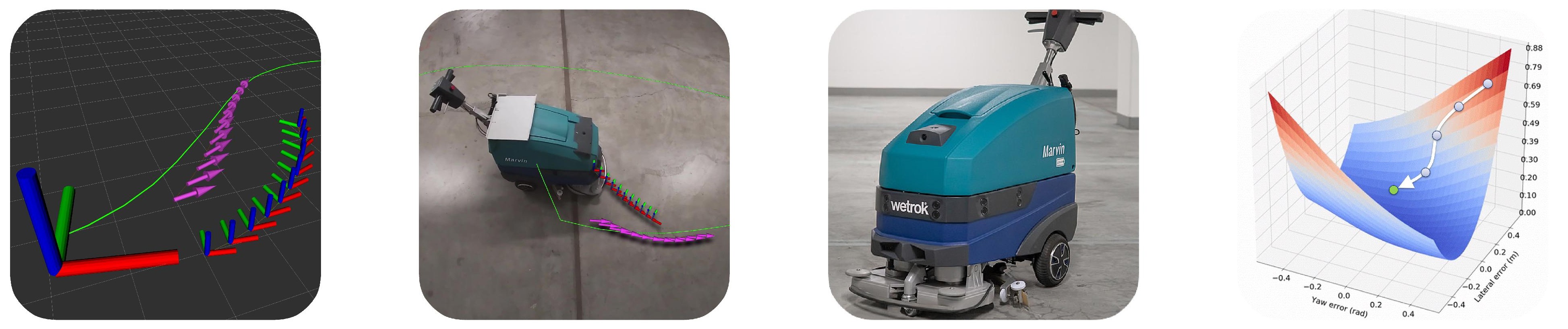
Figure 1: From left to right: simulation of the UGV, the real life UGV platform with visualization overlayed, and lastly an example of a 3D representation of the learned value function.

2 Background

2.1 Notation and Definitions

In this problem setting, we consider an agent within an environment $E$ whose task is to maximize the discounted expected sum of rewards collected from the current time onwards. This is modelled by a Markov Decision Process (MDP) described by the state $\boldsymbol{s}_{t}\in\mathbb{R}^{n_{s}}$ and dynamics $d\boldsymbol{s}=f(\boldsymbol{s}_{t},\boldsymbol{a}_{t})$. At each time step, the agent observes a state $\boldsymbol{s}_{t}$ and takes an action $\boldsymbol{a}_{t}\in\mathbb{R}^{n_{a}}$ according to the policy $\pi(\boldsymbol{s}_{t})$. The environment returns the corresponding evolved observations $\boldsymbol{s}_{t+1}$ , as well as a reward $r_{t}\in\mathbb{R}$. This forms a transition tuple $\langle\boldsymbol{s}_{t},\boldsymbol{a}_{t},r_{t},\boldsymbol{s}_{t+1}\rangle$ for one time step. All transitions are stored in a replay buffer $\mathcal{B}$. The return is defined by the discounted future rewards $R=\sum^{\infty}_{t=0}\gamma^{t}r_{t}(\boldsymbol{s}_{t})$, where the discount factor is $\gamma\in[0,1)$. The value function $V(s)$ describes the expected return of being in state $s$, i.e. $V(s_{0})=\mathbb{E}_{\pi}[R|\,s=\boldsymbol{s}_{0}]$. $V(s)$ is assumed to be time independent. The term cost is used as negative value, rendering minimizing cost an maximising value equivalent statements.

2.2 Model Predictive Control

MPC is a receding horizon control technique that maximizes a value function with respect to a sequence of control actions $\boldsymbol{a}_{0}\dots\boldsymbol{a}_{N-1}$ along a horizon of length $N$. The problem is constrained under state dynamics $\hat{f}(\boldsymbol{x}_{t},\boldsymbol{a}_{t})$, and state and input constraints. Note that here, $\boldsymbol{x}\in\boldsymbol{S}_{k}\subseteq\text{R}^{n_{s}}$ and $\hat{f}(\boldsymbol{x}_{t},\boldsymbol{a}_{t})$ denote the state and state dynamics of the actor respectively, which are distinguished from the true state and state dynamics of the environment. This results in the optimization

$$\pi_{MPC}(\boldsymbol{x}_{0}) =\underset{\boldsymbol{a}_{0},\dots,\boldsymbol{a}_{N-1}}{\arg\max}\,\gamma^{N}g_{N}(\boldsymbol{x}_{N})+\sum^{N-1}_{k=0}\gamma^{k}g(\boldsymbol{x}_{k},\boldsymbol{a}_{k})$$ (1)

s.t. $$\partial_{t}x_{k}=\hat{f}(\boldsymbol{x}_{k},\boldsymbol{a}_{k}),\ \boldsymbol{a}_{k}\in\boldsymbol{A}_{k},\,\boldsymbol{x}_{k}\in\boldsymbol{S}_{k},\ \text{for }k=0,\ldots,N,$$

where $\boldsymbol{x}_{0}\in\text{R}^{n_{s}}$ denotes the current state feedback and $\boldsymbol{a}_{k}\in\boldsymbol{A}_{k}\subseteq\text{R}^{n_{a}}$ the control action, of which only the first is applied. This is then repeated for every control cycle. Notice that this MPC strategy is approximating the initial problem as a finite horizon optimal control problem, which depending on the horizon choice, is not guaranteed to be stable ([Lee2011]). However, as will be seen in Section 3.2, defining the terminal ($g_{N}(\cdot)$) and stage ($g(\cdot)$) costs in terms of the value function allows us to alleviate this limitation.

2.3 Value Function learning

Value function learning is commonly employed in reinforcement learning problems ([sutton2016reinforcement]). In most cases, the value is represented by a state value function it $V_{\theta}(\boldsymbol{s}_{t})$ or an state action value function $Q_{\theta}(\boldsymbol{s}_{t},\boldsymbol{a}_{t})$, parameterized by parameter vector $\theta$. This function is optimized minimizing the mean squared error loss with respect to a learning target, $y_{t}$ :

$$L=\mathbb{E}_{\pi_{\theta}}[(y_{t}-V_{\theta}(\boldsymbol{s}_{t}))^{2}].$$ (2)

3 Method

The presented method is based off the actor-critic framework. The critic captures the global value function represented by a neural network. The actor is represented by a non-linear model predictive controller. The focus lays on the contributions that make it possible to run on a real physical system. The learning algorithm can be found in Appendix LABEL:sec:training_algorithm.

3.1 Critic

The key components to training the critic that are listed next. Note, this does introduce a new set of hyper parameters but were observed to have marginal effect compared to the value function.

Gradient regularization

In the value function loss (Equation 2), we also regularize the Jacobian of the network. Since the Jacobian, $\boldsymbol{J}=\partial_{\boldsymbol{s}}V_{\theta}(\boldsymbol{s})$, and the Hessian of the network are required on the actor side (See Section LABEL:sec:qp_approx), adding such a term will favor a smoother class of functions, which are easier to optimize for QP solvers. Note that the Hessian is often approximated as $\boldsymbol{J}^{T}\boldsymbol{J}$ in the Gauss-Newton Hessian approximation ([bjorck1996numerical]). Therefore, regularizing the Jacobian norm indirectly reduces the Hessian norm, and also aids numerical stability while training. Without this regularization, we found that running MPC with the learned value while training often did not converge. This resulted in unstable behavior, making it difficult to run on a real system.

Experience replay and data augmentation

Experience replay is advantageous in two ways: it increases sample efficiency, and it stabilizes neural network training. This is realized in the form of replay buffer $\mathcal{B}$, see ([silver2014deterministic]). Moreover, we augment our data profiting from the symmetries of the system (e.g. $V_{\theta}(\boldsymbol{x})=V_{\theta}(h(\boldsymbol{x}))$). This not only implies that we can augment our data by the number of symmetries in the system but also that the agent will behave similarly well for symmetric states despite not having visited some of them.

n-step target

An n-step target is employed, it is the bootstrapped sum of discounted rewards over n consecutive steps ([sutton2016reinforcement]):

$$R^{(n)}(\boldsymbol{s}_{t})=\sum^{n-1}_{i=0}\gamma^{i}r(\boldsymbol{s}_{t+i})+\gamma^{n}V_{\theta}(\boldsymbol{s}_{t+n}).$$ (3)

This choice is due to its ability to balance bias and variance which affects Monte-Carlo and TD(0) returns respectively and in practice, it accelerates convergence.

Target network

We maintain a target network $V_{\theta^{\prime}}(s)$ along side the critic network $V_{\theta}(s)$. Effectively, the Polyak-averaged version of the critic’s estimated value function is used for bootstrapping. As shown by [lillicrap2015continuous], this trick greatly improves the actor-critic learning interaction.

3.2 Actor

RL and MPC can be combined in several ways further explained in Section LABEL:sec:related_work. In this section we focus on two methods that employ value function learning.

Terminal Deep Value MPC

The first and most intuitive combination (presented in [lowrey2018plan]) uses the value function as terminal cost for the MPC. They show that bootstrapping the trajectory optimizer with the value function enables it to find global optimal solutions. Indeed, the value provides the missing information about the expected return from the end of the optimization horizon onwards. In this formulation, Equation 1 takes the following form: