Gravastars in $f(\mathbb{T},\mathcal{T})$ gravity

Abstract

We propose a stellar model under the $f(\mathbb{T},\mathcal{T})$ gravity following Mazur-Mottola’s conjecture [1, 2] known as gravastar which is generally believed as a viable alternative to black hole. The gravastar consists of three regions, viz., (I) Interior region, (II) Intermediate shell region, and (III) Exterior region. The pressure within the interior core region is assumed to be equal to the constant negative matter-energy density which provides a constant repulsive force over the thin shell region. The shell is assumed to be made up of fluid of ultrarelativistic plasma and following the Zel’dovich’s conjecture of stiff fluid [3] it is also assumed that the pressure which is directly proportional to the matter-energy density according to Zel’dovich’s conjecture, does cancel the repulsive force exerted by the interior region. The exterior region is completely vacuum and it can be described by the Schwarzschild solution. Under all these specifications we find out a set of exact and singularity-free solutions of the gravastar presenting several physically valid features within the framework of alternative gravity, namely $f(\mathbb{T},\mathcal{T})$ gravity  [4], where the part of the gravitational Lagrangian in the corresponding action is taken as an arbitrary function of torsion scalar $\mathbb{T}$ and the trace of the energy-momentum tensor $\mathcal{T}$.

Managing Editor

1 Introduction

It is generally believed that near the end of the stellar evolution if the mass of the stellar remnant after forming planetary nebula or initiating supernova explosion exceeds three solar mass, then the star continues to collapse due to self gravitational pull leading to highly dense object, i.e., black hole. A very simplest example of it is the Schwarzschild black hole which is assumed to be static as well as uncharged and can be well defined by the following metric (for geometrized units $G=c=1$)

$$ds^{2}=\left(1-\frac{2M}{r}\right)dt^{2}-\left(1-\frac{2M}{r}\right)^{-1}dr^{2}-r^{2}(d\theta^{2}+sin^{2}\theta d\phi^{2}),$$ (1)

where $M$ is the mass of the gravitating object. The metric is singular at $r=0$ (curvature singularity) and $r=2M$ (coordinate singularity). The surface at $r=2M$ which is known as event horizon, prohibits even light to escape from it due to massive gravitational pull.

In order to overcome the problem of singularity as well as to avoid the presence of event horizon Mazur and Mottola [1, 2] first ever proposed the model of gravitatio-nally vacuum star (gravastar) as the alternative to the mysterious end state of gravitationally collapsing star, i.e., black hole which is generally assumed to overcome any kind of repulsive nonthermal pressure of degenerate elementary particle, whatsoever. They generated a new kind of solution by extending the idea of Bose-Einstein condensation and fabricated the model as a cold, dark and compact object with an interior de Sitter condensate phase as well as Schwarzschild exterior. Again these two spacetimes were assumed to be separated by a shell with a small but finite thickness $\ell$ consisting of a stiff fluid with equation of state (EOS) $p=\rho$ [3]. It had also been shown that unlike the black hole the new solution was stable on the basis of thermodynamics and did not possess any information paradox. The entire structure of gravastar can be envisaged with different EOS for the different regions of it as follows:

I. Interior ($0\leq r<r_{1}$): $p=-\rho$,
II. Thin Shell ($r_{1}\leq r\leq r_{2}$ ): $p=+\rho$,
III. Exterior ($r_{2}<r$): $p=\rho=0$.

One can find plenty of works related to gravastar based on different mathematical and physical issues as available in literature. Most of these works have been done in the framework of Einstein’s general relativity (GR) [1, 2, 5, 6, 7, 8, 9, 10, 11, 12, 13, 14, 15, 16, 17, 18, 19, 20, 21, 22]. Now-a-days Einstein’s general relativity presents some shortcomings in theoretical as well as observational aspects. In general relativity we often encounter the presence of singularities and there is a lack of self-consistent theory of quantum gravity. Also, from the observational point of view GR is incapable to address galactic, extra-galactic and cosmic dynamics without the consideration of the presence of exotic form of matter-energy which are often known as dark matter and dark energy [23, 24, 25, 26]. Alternatively, in spite of changing the source side of the Einstein field equations one can equally ask to modify the gravitational sector to describe the galactic as well as cosmic dynamics such as late-time acceleration of the Universe etc. As a result several modified theories of gravitation such as $f(R)$ gravity, $f(\mathbb{T})$ gravity, $f(R,\mathcal{T})$ gravity etc. have been proposed from time to time. In all these theories the geometrical part have been changed by taking a generalized functional form of the argument as the gravitational Lagrangian in the corresponding action. In modified theories of gravity one usually generalizes the corresponding action on the basis of curvature description of gravity. Interestingly, one can modify the corresponding action based on torsion, but not on curvature as was first done by Einstein himself and that is known as the “Teleparallel Equivalent of General Relativity” (TEGR) where the gravity is described by torsion tensor and not by curvature [27, 28, 29, 30, 31, 33, 32, 34, 35, 36, 37]. One can further modify TEGR by extending $\mathbb{T}$ to an arbitrary function in the Lagrangian [38, 39, 40].

Moreover, it is possible to modify the general relativity by coupling the geometric sector with the non-geometric sector  [41, 42, 43, 44, 45]. Furthermore, in another modification one can consider the coupling of the matter Lagrangian to the Ricci scalar [46, 47, 48] and extend it to the arbitrary function of $(R,\mathcal{L}_{m})$ [49, 50, 51, 52, 53]. Also, one may consider the models where Ricci scalar $R$ is coupled to the trace of the energy-momentum tensor $\mathcal{T}$ and further extend it to an arbitrary function such as in $f(R,\mathcal{T})$ theory [54].

Similarly, starting from TEGR but not from GR, it is also possible to consider the matter-coupled modified gravity theory. One of such theories, namely $f(\mathbb{T},\mathcal{T})$ gravity, has been first proposed by Harko et al. [4]. In this modified theory the part of the gravitational Lagrangian is taken as an arbitrary function of torsion scalar $\mathbb{T}$ and the trace of the energy-momentum tensor $\mathcal{T}$. Comparing with the other theories based on the formalism of curvature or torsion, $f(\mathbb{T},\mathcal{T})$ seems to be a completely different modification for describing the gravity. In this paper, we study the gravastar model under $f(\mathbb{T},\mathcal{T})$ gravity, being motivated by the previous successful work of Das et al. on compact star [55, 56] as well as gravastar [57] under alternative formalism of GR.

Most of the works under the background of $f(\mathbb{T},\mathcal{T})$ gravity have been done in different cosmological realm as available in literature [58, 59, 60, 61, 62, 63, 64, 65, 66]. Though there are a few astrophysical applications of $f(\mathbb{T},\mathcal{T})$ gravity which can be found in Refs. [67, 68]. Under the backgound of $f(\mathbb{T},\mathcal{T})$ gravity Pace and Said [67] have derived the working model for the Tolman-Oppenheimer-Volkoff (TOV) equation for quark star incorporating the MIT bag model whereas in another work [68] they have derived the TOV equation in neutron star systems using a perturbative approach.

The outline of the present investigation is as follows: In Sec. 2 the basic mathematical formalism of $f(\mathbb{T},\mathcal{T})$ theory has been presented as the background study. The explicit form of field equations along with the conservation equation of $f(\mathbb{T},\mathcal{T})$ gravity for the specific form of gravitational Lagrangian is provided in Sec. 3 whereas in Sec. 4 we obtain the solutions of the field equations considering the different regions, viz., interior region, exterior region and the shell region of the gravastar. In Sec. 5 we discuss the matching conditions in order to determine the numerical values of several constants which have arisen in different calculations. Sec. 6 deals with some physical features, i.e., proper length, pressure, energy and entropy within the shell region. . Junction conditions are presented in Sec. 7 and finally, we pass some concluding remarks in Sec. 8.

2 Basic Mathematical Formalism of $f(\mathbb{T},\mathcal{T})$ Theory

The modified theories of Tele-Parallel gravity are those for which the scalar torsion of Tele-Parallel action is substituted by an arbitrary function of this latter. As it is done in Tele-Parallel, the modified versions of this theory are also described by the orthonormal tetrads and it’s components are defined on the tangent space of each point of the manifold. The line element is written as

$$ds^{2}=g_{\mu\nu}dx^{\mu}dx^{\nu}=\eta_{ij}\theta^{i}\theta^{j},$$ (2)

with the following definitions

$$dx^{\mu}=e_{i}^{\;\;\mu}\theta^{i};\,\quad\theta^{i}=e^{i}_{\;\;\mu}dx^{\mu}.$$ (3)

Note that $\eta_{ij}=diag(1,-1,-1,-1)$ is the Minkowskian metric and the $\{e^{i}_{\;\mu}\}$ are the components of the tetrad which satisfy the following identity:

$$e^{\;\;\mu}_{i}e^{i}_{\;\;\nu}=\delta^{\mu}_{\nu},\quad e^{\;\;i}_{\mu}e^{\mu}_{\;\;j}=\delta^{i}_{j}.$$ (4)

In GR one use the following Levi-Civita’s connection

$$\bar{\Gamma}{}_{\;\;\mu\nu}^{\rho}=\frac{1}{2}g^{\rho\sigma}\left(\partial_{\nu}g_{\sigma\mu}+\partial_{\mu}g_{\sigma\nu}-\partial_{\sigma}g_{\mu\nu}\right),$$ (5)

which preserves the curvature whereas the torsion vanishes. But in the Tele-Parallel theory and its modified version, one keeps the scalar torsion by using Weizenbock’s connection defined as

$$\Gamma^{\lambda}_{\mu\nu}=e^{\;\;\lambda}_{i}\partial_{\mu}e^{i}_{\;\;\nu}=-e^{i}_{\;\;\mu}\partial_{\nu}e_{i}^{\;\;\lambda}.$$ (6)

From this connection, one obtains the geometric objects. The first is the torsion as defined by

$$T^{\lambda}_{\;\;\;\mu\nu}=\Gamma^{\lambda}_{\mu\nu}-\Gamma^{\lambda}_{\nu\mu},$$ (7)

from which we define the second object contorsion defined as

$$K_{\;\;\mu\nu}^{\lambda}\equiv\Gamma_{\;\mu\nu}^{\lambda}-\bar{\Gamma}{}_{\;\mu\nu}^{\lambda}=\frac{1}{2}(T_{\mu}{}^{\lambda}{}_{\nu}+T_{\nu}{}^{\lambda}{}_{\mu}-T_{\;\;\mu\nu}^{\lambda}),$$ (8)

where the expression $\bar{\Gamma}{}_{\;\;\mu\nu}^{\lambda}$ designs the above defined connection. Then we can write

$$K^{\mu\nu}_{\;\;\;\;\lambda}=-\frac{1}{2}\left(T^{\mu\nu}_{\;\;\;\lambda}-T^{\nu\mu}_{\;\;\;\;\lambda}+T^{\;\;\;\nu\mu}_{\lambda}\right).$$ (9)

The two previous geometric objects (the torsion and the contorsion) are used to define another tensor by

$$S_{\lambda}^{\;\;\mu\nu}=\frac{1}{2}\left(K^{\mu\nu}_{\;\;\;\;\lambda}+\delta^{\mu}_{\lambda}T^{\alpha\nu}_{\;\;\;\;\alpha}-\delta^{\nu}_{\lambda}T^{\alpha\mu}_{\;\;\;\;\alpha}\right).$$ (10)

The torsion scalar is usually constructed from torsion and contorsion as follows:

$$\mathbb{T}=S_{\sigma}^{~{}\mu\nu}T^{\sigma}_{~{}\mu\nu}.$$ (11)

In the modified versions of Tele-Parallel gravity, one can use a general algebraic function of scalar torsion instead of the scalar torsion only as it is done in the initial theory. So, the modified action [4] can be written as

$$\mathbb{S}=\int d^{4}xe\left[\frac{\mathbb{T}+f(\mathbb{T},\mathcal{T})}{16\pi}+\mathcal{L}_{m}\right].$$ (12)

Varying the action with respect to the tetrad, one obtains the equations of motion [4] as

$$[\partial_{\xi}(ee^{\rho}_{a}S^{\;\;\sigma\xi}_{\rho})-ee^{\lambda}_{a}S^{\rho\xi\sigma}T_{\rho\xi\lambda}](1+f_{\mathbb{T}})+ee^{\rho}_{a}(\partial_{\xi}\mathbb{T})S^{\;\;\sigma\xi}_{\rho}f_{\mathbb{T}\mathbb{T}}+\frac{1}{4}ee^{\sigma}_{a}(\mathbb{T})=$$

$$-\frac{1}{4}ee^{\sigma}_{a}f-ee^{\rho}_{a}(\partial_{\xi}\mathcal{T})S^{\;\;\sigma\xi}_{\rho}f_{\mathbb{T}\mathcal{T}}+f_{\mathcal{T}}\;\left(\frac{e\,T^{\sigma}_{\;\;a}+ee^{\sigma}_{a}\;p}{2}\right)+4\pi\,e\,T^{\sigma}_{\;\;a}\;,$$ (13)

with $f_{\mathcal{T}}=\partial f/\partial\mathcal{T}$, $f_{\mathbb{T}}=\partial f/\partial\mathbb{T}$, $f_{\mathbb{T}\mathcal{T}}=\partial^{2}f/\partial\mathbb{T}\partial\mathcal{T}$, $f_{\mathbb{T}\mathbb{T}}=\partial^{2}f/\partial\mathbb{T}^{2}$ and $T^{\sigma}_{\;\;a}$ is the energy-momentum tensor of matter field where we assume the energy-momentum tensor to be that of a perfect fluid, i.e.,

$$T_{\mu\nu}=(\rho+p)u_{\mu}u_{\nu}-pg_{\mu\nu}.$$ (14)

After some contraction, we can rewrite the first term on the R.H.S. of Eq. (13) as follows [69]:

$$e^{a}_{\nu}e^{-1}\partial_{\xi}(ee^{\rho}_{a}S^{\;\;\sigma\xi}_{\rho})-S^{\rho\xi\sigma}T_{\rho\xi\nu}=-\nabla^{\xi}S_{\nu\xi}^{\;\;\;\;\sigma}-S^{\xi\rho\sigma}K_{\rho\xi\nu},$$ (15)

and one can have

$$G_{\mu\nu}-\frac{1}{2}\,g_{\mu\nu}\,\mathbb{T}=-\nabla^{\rho}S_{\nu\rho\mu}-S^{\sigma\rho}_{\;\;\;\;\mu}K_{\rho\sigma\nu}.$$ (16)

Hence from the combination of Eqs. (15) and (16), the field equation of Eq. (2) can be written as

$$A_{\mu\nu}(1+f_{\mathbb{T}})+\frac{1}{4}g_{\mu\nu}\;\mathbb{T}=B_{\mu\nu}^{eff},$$ (17)

where

$$A_{\mu\nu}=g_{\sigma\mu}e^{a}_{\nu}[e^{-1}\partial_{\xi}(ee^{\rho}_{a}S^{\;\;\sigma\xi}_{\rho})-e^{\lambda}_{a}S^{\rho\xi\sigma}T_{\rho\xi\lambda}]=-\nabla^{\sigma}S_{\nu\sigma\mu}-S_{\;\;\;\;\mu}^{\rho\lambda}K_{\lambda\rho\nu}=G_{\mu\nu}-\frac{1}{2}g_{\mu\nu}\mathbb{T}$$ (18)

and

$$B_{\mu\nu}^{eff}=S^{\rho}_{\;\;\;\mu\nu}\;f_{\mathbb{T}\mathcal{T}}\;\partial_{\rho}\mathcal{T}-S^{\rho}_{\;\;\;\mu\nu}\;f_{\mathbb{T}\mathbb{T}}\;\partial_{\rho}\mathbb{T}-\frac{1}{4}g_{\mu\nu}f+f_{\mathcal{T}}\;\Big{(}\frac{T_{\mu\nu}+g_{\mu\nu}\;p}{2}\Big{)}+4\pi T_{\mu\nu}.$$ (19)

So Eq. (17) takes the following form

$$(1+f_{\mathbb{T}})\,G_{\mu\nu}=T_{\mu\nu}^{eff},$$ (20)

where

$$T_{\mu\nu}^{eff}=S^{\rho}_{\;\;\;\mu\nu}\;f_{\mathbb{T}\mathcal{T}}\;\partial_{\rho}\mathcal{T}-S^{\rho}_{\;\;\;\mu\nu}\;f_{\mathbb{T}\mathbb{T}}\;\partial_{\rho}\mathbb{T}+\frac{1}{4}g_{\mu\nu}\Big{(}\mathbb{T}-f\Big{)}+\frac{\mathbb{T}\,g_{\mu\nu}\,f_{\mathbb{T}}}{2}$$

$$+f_{\mathcal{T}}\;\Big{(}\frac{T_{\mu\nu}+g_{\mu\nu}\;p}{2}\Big{)}+4\pi T_{\mu\nu}\;.$$ (21)

The covariant derivative of Eq. (20) reads as

$$\nabla^{\mu}\Big{[}(1+f_{\mathbb{T}})\,G_{\mu\nu}\Big{]}=\nabla^{\mu}T_{\mu\nu}^{eff}=\nabla^{\mu}\Bigg{[}\frac{\mathbb{T}\,g_{\mu\nu}\,f_{\mathbb{T}}}{2}+S^{\rho}_{\;\;\;\mu\nu}\;f_{\mathbb{T}\mathcal{T}}\;\partial_{\rho}\mathcal{T}-S^{\rho}_{\;\;\;\mu\nu}\;f_{\mathbb{T}\mathbb{T}}\;\partial_{\rho}\mathbb{T}$$ (22)

$$+ \frac{1}{4}g_{\mu\nu}\Big{(}\mathbb{T}-f\Big{)}+f_{\mathcal{T}}\;\Big{(}\frac{T{\mu\nu}+g_{\mu\nu}\;p}{2}\Big{)}+4\pi T_{\mu\nu}\Big{]}.$$

The previous equation leads to the following expression

$$\nabla^{\mu}T_{\mu\nu} = \frac{-2}{(f_{\mathcal{T}}+8\pi)}\Bigg{\{}\nabla^{\mu}\Big{[}\frac{\mathbb{T}\,g_{\mu\nu}\,f_{\mathbb{T}}}{2}+S^{\rho}_{\;\;\;\mu\nu}\;f_{\mathbb{T}\mathcal{T}}\;\partial_{\rho}\mathcal{T}-S^{\rho}_{\;\;\;\mu\nu}\;f_{\mathbb{T}\mathbb{T}}\;\partial_{\rho}\mathbb{T}+\frac{1}{4}g_{\mu\nu}\Big{(}\mathbb{T}-f\Big{)}\Big{]}$$ (23)

$$+ \Big{(}\frac{T_{\mu\nu}+g_{\mu\nu}\;p}{2}\Big{)}\,\nabla^{\mu}f_{\mathcal{T}}+\frac{f_{\mathcal{T}}}{2}\,\nabla^{\mu}(g_{\mu\nu}\;p)-G_{\mu\nu}\nabla^{\mu}(1+f_{\mathbb{T}})\Bigg{\}}.$$

We have taken the functional form of $f(\mathbb{T},\mathcal{T})$ as $f(\mathbb{T},\mathcal{T})=g_{1}(\mathbb{T})+g_{2}(\mathcal{T})$ where for simplicity we have chosen $g_{1}(\mathbb{T})=0$ and $g_{2}(\mathcal{T})=2Q\mathcal{T}$ so that $f_{\mathbb{T}}=f_{\mathbb{T}\mathbb{T}}=f_{\mathbb{T}\mathcal{T}}=0$.

For the above form of $f(\mathbb{T},\mathcal{T})$ the Eq. (23) reduces to

$$\nabla^{\mu}T^{\mu}_{\nu}=\frac{1}{(f_{\mathcal{T}}+8\pi)}\Bigg{\{}\frac{1}{2}\delta^{\mu}_{\nu}\nabla^{\mu}f(\mathbb{T},\mathcal{T}) - \Big{(}T^{\mu}_{\nu}+\delta^{\mu}_{\nu}\;p\Big{)}\,\nabla^{\mu}f_{\mathcal{T}}-f_{\mathcal{T}}\,\delta^{\mu}_{\nu}\nabla^{\mu}\,p\Bigg{\}}.$$ (24)

3 The field equations in $f(\mathbb{T},\mathcal{T})$ gravity

Assuming that the manifold to be static and spherically symmetric, the metric can be written as

$$ds^{2}=e^{\nu(r)}dt^{2}-e^{\lambda(r)}dr^{2}-r^{2}\left(d\theta^{2}+\sin^{2}\theta d\phi^{2}\right).$$ (25)

In order to re-write the line element Eq. (25) into the invariant form under the Lorentz transformations as in Eq. (2), we define the tetrad matrix $[e^{i}_{\;\mu}]$ as

$$\left[e^{i}_{\;\;\mu}\right]=diag\left[e^{\nu(r)/2},e^{\lambda(r)/2},r,r\sin\theta\right].$$ (26)

From Eq. (26), one can obtain $e=\det{\left[e^{i}_{\;\;\mu}\right]}=e^{(\nu+\lambda)/2}r^{2}\sin\theta$ and using Eq. (11) the torsion scalar can be written as

$$\mathbb{T}(r)=\frac{2e^{-\lambda}}{r}\left(\nu^{\prime}+\frac{1}{r}\right).$$ (27)

Now the nonzero components of the Einstein tensors can be written as

$$G_{0}^{0}=\frac{e^{-\lambda}}{r^{2}}(-1+e^{\lambda}+\lambda^{\prime}r),$$ (28)

$$G_{1}^{1}=\frac{e^{-\lambda}}{r^{2}}(-1+e^{\lambda}-\nu^{\prime}r),$$ (29)

$$G_{2}^{2}=G_{3}^{3}=\frac{e^{-\lambda}}{4r}[2(\lambda^{\prime}-\nu^{\prime})-(2\nu^{\prime\prime}+\nu^{\prime 2}-\nu^{\prime}\lambda^{\prime})r],$$ (30)

where primes stand for derivative with respect to the radial co-ordinate $r$.

For the functional form of $f(\mathbb{T},\mathcal{T})$ as $f(\mathbb{T},\mathcal{T})=g_{1}(\mathbb{T})+g_{2}(\mathcal{T})$ with $g_{1}(\mathbb{T})=0$ the field Eq. (20) takes the form

$$(1+0)G_{00} = T_{00}^{eff},$$ (31)

$$(1+0)G_{11} = T_{11}^{eff},$$ (32)

$$(1+0)G_{22} = T_{22}^{eff},$$ (33)

$$(1+0)G_{33} = T_{33}^{eff},$$ (34)

where

$$T_{0}^{0~{}eff}=\frac{1}{4}\left(\mathbb{T}-f\right)+\left(4\pi+\frac{f_{\mathcal{T}}}{2}\right)\rho+\frac{pf_{\mathcal{T}}}{2},$$ (35)

$$T_{1}^{1~{}eff}=T_{2}^{2~{}eff}=T_{3}^{3~{}eff}=\frac{1}{4}\left(\mathbb{T}-f\right)-4\pi\,p.$$ (36)

Finally, we have the following field equations:

$$-\frac{3e^{-\lambda}}{2r^{2}}+\frac{1}{r^{2}}+\frac{e^{-\lambda}}{r}\left(\lambda^{\prime}-\frac{\nu^{\prime}}{2}\right)=\rho\left(4\pi+\frac{Q}{2}\right)+\frac{5Qp}{2},$$ (37)

$$-\frac{3e^{-\lambda}}{2r^{2}}+\frac{1}{r^{2}}-\frac{3\nu^{\prime}e^{-\lambda}}{2r}=p\left(\frac{3Q}{2}-4\pi\right)-\frac{Q\rho}{2},$$ (38)

$$\frac{\lambda^{\prime}e^{-\lambda}}{2r}-\frac{3\nu^{\prime}e^{-\lambda}}{2r}-\frac{e^{-\lambda}}{4}\left(2\nu^{\prime\prime}+\nu^{\prime 2}-\nu^{\prime}\lambda^{\prime}\right)-\frac{e^{-\lambda}}{2r^{2}}=p\left(\frac{3Q}{2}-4\pi\right)-\frac{Q\rho}{2}.$$ (39)

Also the conservation equation in $f(T,\mathcal{T})$ gravity takes the form as follows

$$\frac{1}{2}(p+\rho)\nu^{\prime}+p^{\prime}=\frac{Q}{(8\pi+2Q)}(5p^{\prime}-\rho^{\prime}).$$ (40)

4 The solutions of the field equations for different regions of the gravastar

4.1 Interior Space-time

Following the prescription of Mazur and Mottola [1, 2] we have the EOS that represent the interior region of the gravastar is given by

$$p=-\rho.$$ (41)

Now using Eqs. (40) and (41) we have obtained the matter density and pressure within the shell as

$$p=-\rho=-\rho_{c},$$ (42)

where $\rho_{c}$ is a constant, i.e., the matter density as well as pressure inside the shell remain constant. This indicates that the pressure and the density is homogeneous and isotropic inside the gravastar.

Now using Eqs. (37) and (38) and putting the condition provided in Eq. (41) we can find the metric function $e^{-\lambda}$ for the interior spacetime of the gravastar as

$$e^{-\lambda}=\frac{2}{3}-\frac{4\rho_{c}(2\pi-Q)r^{2}}{9}+\frac{c_{1}}{r},$$ (43)

where $c_{1}$ is a constant of integration. To make the solution regular at the centre of the gravastar, i.e., at $r=0$ we have to set $c_{1}$ to zero so that

$$e^{-\lambda}=\frac{2}{3}-\frac{4\rho_{c}(2\pi-Q)r^{2}}{9}.$$ (44)

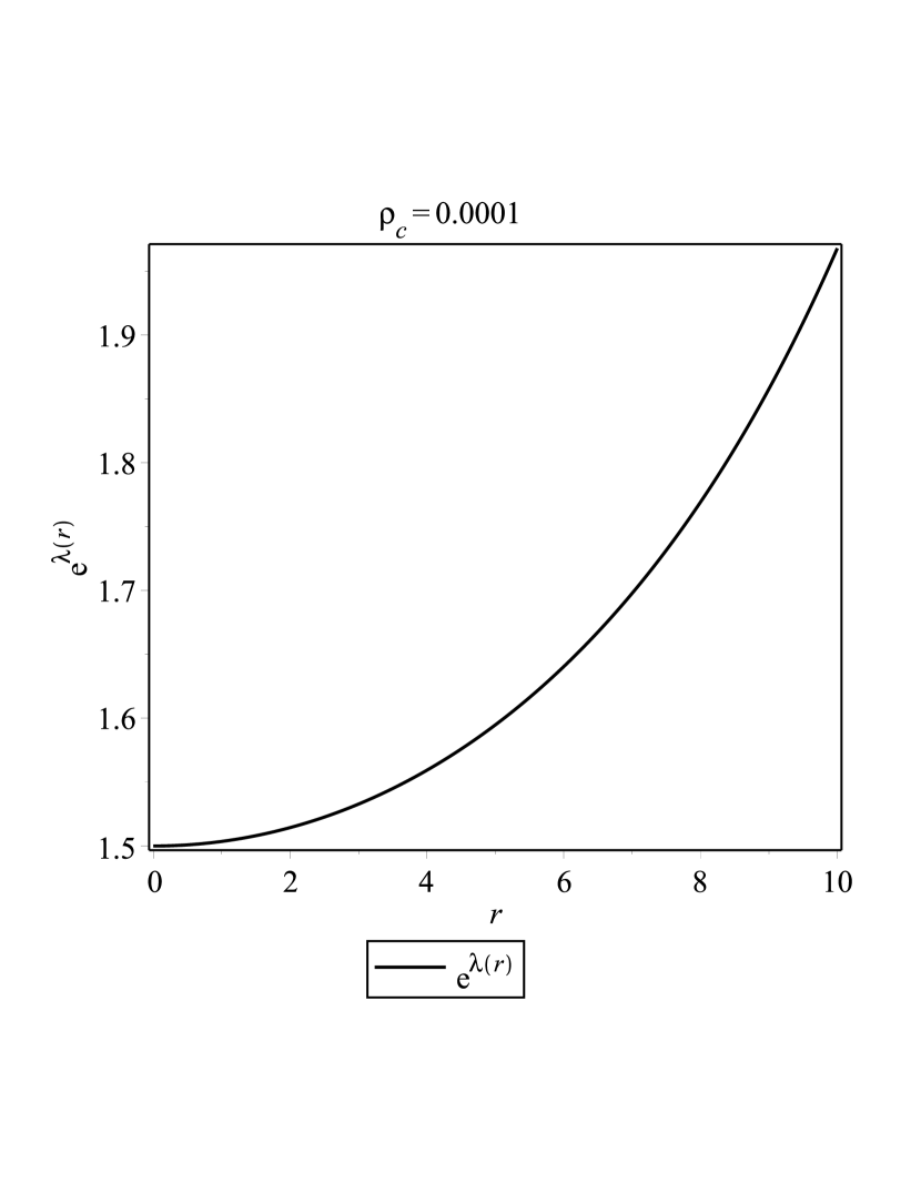
Figure 1: Variation of the metric function ($e^{\lambda(r)}$) within the interior region with respect to $r$ (km).

Now putting the above expression in Eq. (38) we get

$$e^{\nu}=c_{2}\left[2\rho_{c}(2\pi-Q)r^{2}-3\right]^{\frac{3\pi-2Q}{2\rho_{c}(2\pi-Q)}},$$ (45)

where $c_{2}$ is an integration constant. From the above solutions as written by the Eqs. (44) and (45) one can observe that both solutions are regular at the center (i.e., $r=0$) of the gravastar which means solutions have no singularity at the center.

Now one can calculate the active gravitational mass of the interior of the gravastar as

$$\tilde{M}=\int_{0}^{R}4\pi r^{2}\rho dr=\frac{4}{3}\pi R^{3}\rho_{c},\\$$ (46)

where $r=R$ is the internal radius of the gravastar.

4.2 Intermediate thin shell

The shell has been formed within the intermediate region of two spacetimes, namely, the interior and the exterior spacetime. The thickness of the shell is very small but finite and it contains the entire matter of the collapsing star. In connection to the cold, compact baryonic universe, this type of ultra relativistic matter can be termed as the stiff fluid which was first introduced by Zel’dovich [3]. This type of fluid obeys the EOS $p=\rho$ which means it provides the necessary balancing force to counter the repulsion from the interior keeping the system in stable equilibrium.

In the present scenario we can set up an argument that it may happen from thermal excitations at $0$ K temperature with negligible chemical potential or from the conserved number density of the gravitational quanta [1, 2]. In many cosmological and astrophysical studies various researchers have used this type of fluid [70, 71, 72] for feasible explanations.

Now we are looking for the mathematical as well as physical acceptable solution to explain the formation of the shell. It is very difficult to obtain the exact solution of the field equations within the nonvacuum region using the EOS $p=\rho$. However, considering the framework of thin shell approximation, we can find the analytical solution of the shell. Therefore, we have considered $e^{-\lambda}$ lying between the range $0<e^{-\lambda}\ll 1$. Following the prescription of Israel [74] we can have an argument regarding the formation of shell at the intermediate region of the two spacetimes (here the vacuum interior and Schwarzschild exterior).

Now with the thin shell approximation, the field Eqs. (37)-(39) can be written as

$$\frac{1}{r^{2}}+\frac{e^{-\lambda}\lambda^{\prime}}{r}=\rho\left(4\pi+\frac{Q}{2}\right)+\frac{5Qp}{2},$$ (47)

$$\frac{1}{r^{2}}=p\left(\frac{3Q}{2}-4\pi\right)-\frac{Q\rho}{2},$$ (48)

$$\frac{e^{-\lambda}\lambda^{\prime}}{2r}+\frac{e^{-\lambda}\nu^{\prime}\lambda^{\prime}}{4}=p\left(\frac{3Q}{2}-4\pi\right)-\frac{Q\rho}{2}.$$ (49)

From Eq. (48) we can calculate the metric function $e^{-\lambda}$ as

$$e^{-\lambda}=k_{1}+2\left(\frac{4\pi+Q}{4\pi-Q}\right)\ln r,$$ (50)

where $k_{1}$ is a constant of integration which can be calculated using the matching condition between the thin shell region and the exterior vacuum region.

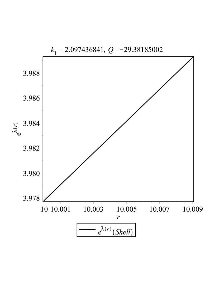
Figure 2: Variation of $e^{\lambda(r)}$ within the shell with respect to $r$ (km).

Now using Eqs. (49) and (50) we have found the other metric potential $e^{\nu}$ as

$$e^{\nu}=k_{2}r^{-\frac{16\pi}{Q+4\pi}},$$ (51)

where $k_{2}$ is also a constant of integration. Variation of $e^{\nu(r)}$ has been studied and found to be similar in its nature as Fig. 2.

4.3 Exterior region

The exterior of the gravastar is assumed to obey the EOS $p=\rho=0$ which means that the outside region of the shell is completely vacuum. The corresponding line-element can be written as

$$ds^{2}=\left(1-\frac{2M}{r}\right)dt^{2} - \left(1-\frac{2M}{r}\right)^{-1}dr^{2}-r^{2}(d\theta^{2}+\sin^{2}\theta d\phi^{2}),$$ (52)

which is same as in Schwarzschild type vacuum solution in $(3+1)$ dimension. Here $M$ is the total mass of the gravastar.

5 Matching Condition

To determine the value of the integration constant $k_{1}$ we have matched the metric potential at the junction of interior region and the shell. We have obtained

$$k_{1}=1-\frac{2M}{R_{2}}+2\left(\frac{Q+4\pi}{Q-4\pi}\right)\ln R_{2}.$$ (53)

We have calculated the value of the other integration constant by matching the metric potentials at the junction of the shell and the exterior region of the gravastar as

$$k_{2}=\left(1-\frac{2M}{R_{2}}\right)R_{2}^{\frac{16\pi}{4\pi+Q}}.$$ (54)

The expression of $Q$, using the continuity condition of $\frac{\delta g_{tt}}{\delta r}$ at the junction of the shell, can be found as

$$Q=\frac{1}{2}\frac{R_{2}\pi(-16+\frac{32M}{R_{2}})}{M}-4\pi.$$ (55)

In the present paper we have used the total mass of the gravastar $M=3.75M_{\odot}$ ($M_{\odot}$ is the solar mass), internal radius $R_{1}=10$ km and the thickness of the shell, i.e., $\epsilon=R_{2}-R_{1}=0.009$ km and $\rho_{c}=0.0001$ [73]. Using these values we have determined $k_{1}$, $k_{2}$, and $Q$ as $2.097436841$, $0.2562733037\times 10^{-3}$ and $-29.38185002$ respectively.

6 Physical features of the shell

6.1 Proper Thickness

According to the conjecture of Mazur and Mottola [1, 2], the stiff fluid of the shell is situated between the junction of two spacetimes. The length span of the shell is from $r=R$ (i.e., the phase boundary between the interior and the shell) to $r=R+\epsilon$ (i.e., the phase boundary between the shell and the exterior spacetime). So, one can calculate the proper thickness between these two interfaces and proper length or the proper thickness of the shell can be determined using the following formula

$$\ell = \int^{R+\epsilon}_{R}\frac{dr}{\sqrt{e^{-\lambda}}}=\int^{R+\epsilon}_{R}\frac{dr}{\sqrt{k_{1}+2\left(\frac{4\pi+Q}{4\pi-Q}\right)\log r}}$$ (56)

$$= \left[\frac{e^{-\frac{k_{1}}{b}}erfc\left[-\sqrt{\frac{k_{1}+b\log r}{b}}\right]\sqrt{-\frac{k_{1}+b\log r}{b}}}{\sqrt{k_{1}+b\log r}}\right]_{R}^{R+\epsilon},$$

where $b=2\left(\frac{4\pi+Q}{4\pi-Q}\right)$ and $erfc$ is the complementary error function which can be defined for a variable $z$ as

$$erfc(z)=\frac{\Gamma(\frac{1}{2},z^{2})}{\sqrt{\pi}}.$$ (57)

It has been observed that the proper length within the shell remains positive and

finite whose variation found to be similar to that of the matter density.

6.2 Pressure and density

From Eqs. (40) and (51) we obtain the matter density as well as the pressure of the shell as

$$\rho=p=k_{3}(e^{-\nu})^{\frac{4\pi+Q}{4\pi-Q}}=k_{3}k_{2}^{\frac{Q+4\pi}{Q-4\pi}}r^{\frac{16\pi}{4\pi-Q}}=\rho_{0}r^{\frac{16\pi}{4\pi-Q}},$$ (58)

where $k_{3}$ is an integration constant and $\rho_{0}=k_{3}k_{2}^{(\frac{Q+4\pi}{Q-4\pi})}$ is also constant. From the above equation one can see that the matter density increases with $r$ over the shell. Eq. (58) suggests that the density of the shell must be very high. The variation of the density in Fig. 3 also indicates that it increases from the interior boundary to the exterior boundary, i.e., the shell is more compact at the junction of exterior region than that of the interior region.

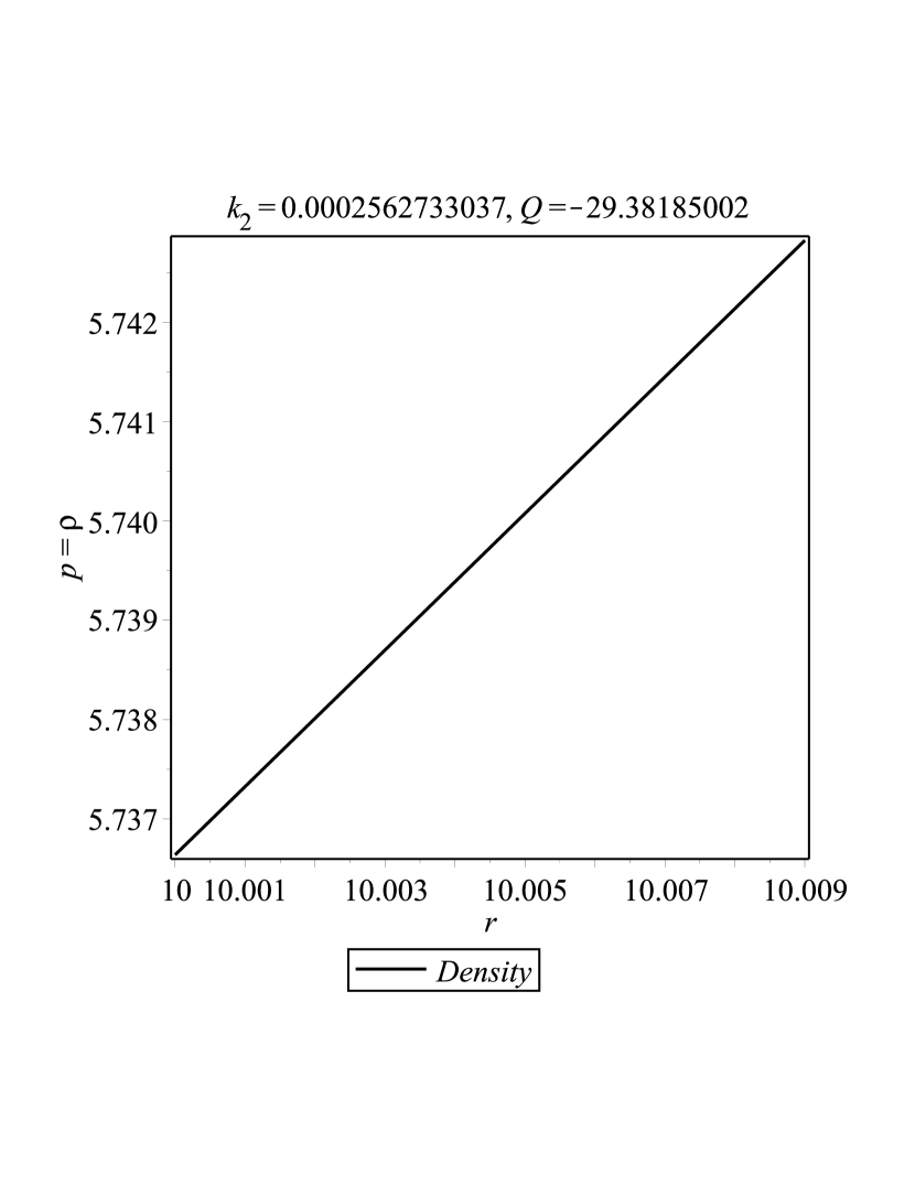
Figure 3: Variation of the matter density ($\rho$) of the shell with respect to $r$ (km).

6.3 Energy

We calculate the energy content within the thin shell as

$$E=\int^{R+\epsilon}_{R}4\pi r^{2}\rho dr=\int^{R+\epsilon}_{R}4\pi r^{2}\rho_{0}r^{\frac{16\pi}{Q+4\pi}}dr=\frac{4\pi\rho_{0}(4\pi-Q)}{28\pi-3Q}\left[r^{\frac{28\pi-3Q}{4\pi-Q}}\right]_{R}^{R+\epsilon}.$$ (59)

It has been verified that variation of the energy with respect to the radial parameter $r$ shows similar nature as the matter density within the shell.

6.4 Entropy

The entropy within the thin shell can be obtained using the following equation as

$$S=\int^{R+\epsilon}_{R}4\pi r^{2}\frac{s(r)}{\sqrt{e^{-\lambda}}}dr,$$ (60)

where $s(r)$ is the entropy density.

So, following Mazur and Mottola [1, 2] we can write it as follows

$$s(r)=\frac{\xi^{2}k_{B}^{2}T(r)}{4\pi\hbar^{2}}=\xi\frac{k_{B}}{\hbar}\sqrt{\frac{p}{2\pi}},$$ (61)

where $\xi$ is a dimensionless constant.

Inserting Eq. (61) in Eq. (60) one can calculate the entropy of the fluid within the shell as

$$S = \frac{4\pi\xi k_{B}}{\hbar\sqrt{2\pi}}\int^{R+\epsilon}_{R}r^{2}\sqrt{\frac{p}{e^{-\lambda}}}dr=\frac{\xi k_{B}\sqrt{8\pi}}{\hbar}\int^{R+\epsilon}_{R}r^{2}\sqrt{\frac{\rho_{0}r^{\frac{16\pi}{4\pi-Q}}}{k_{1}+2\left(\frac{4\pi+Q}{4\pi-Q}\right)\ln r}}dr$$ (62)

$$= \frac{\xi k_{B}\sqrt{8\pi\rho_{0}}}{\hbar b\sqrt{-\frac{(6+c)(k_{1}+\log r)}{b}}}\left[e^{-\frac{k_{1}(c+b)}{2b}}\sqrt{2\pi(k_{1}+\log r)}\right.\left.erfc\left[-\frac{(3+\frac{c}{2})(k_{1}+b\log r)}{b}\right]\right]_{R}^{R+\epsilon},$$

where $c={16\pi}/(4\pi-Q)$. In Planckian units we have $k_{B}=\hbar=1$. The variation of the entropy over the thin shell has been shown in Fig. 4.

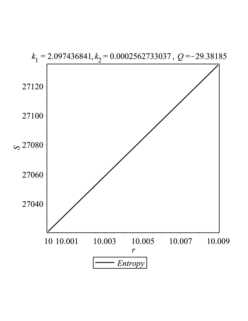
Figure 4: Variation of the entropy ($S$) of the shell with respect to $r$ (km).

7 Junction Condition

We have three segments of the gravastar, the shell of the gravastar is formed between the junction of two spacetimes, i.e., the interior and the exterior regions. Using the condition of Darmois-Israel [75, 74] we calculate the surface stresses at the junction interface. The intrinsic surface stress energy tensor $S_{ij}$ is given by the Lanczos equation [76, 77, 78, 79] in the following form

$$S_{j}^{i}=-\frac{1}{8\pi}(K_{j}^{i}-\delta_{j}^{i}K_{k}^{k}),$$ (63)

the discontinuity in the second fundamental form is given by

$$K_{ij}=K_{ij}^{+}-K_{ij}^{-},$$ (64)

where the second fundamental form is given by

$$K_{ij}^{\pm}=-n_{\nu}^{\pm}\left[\frac{\partial^{2}X_{\nu}}{\partial\xi^{i}\partial\xi^{j}}+\Gamma_{\alpha\beta}^{\nu}\frac{\partial X^{\alpha}}{\partial\xi^{i}}\frac{\partial X^{\beta}}{\partial\xi^{j}}\right]|_{S},$$ (65)

where the unit normal vector $n_{\nu}^{\pm}$ are defined as

$$n_{\nu}^{\pm}=\pm\left|g^{\alpha\beta}\frac{\partial f}{\partial X^{\alpha}}\frac{\partial f}{\partial X^{\beta}}\right|^{-\frac{1}{2}}\frac{\partial f}{\partial X^{\nu}},$$ (66)

with $n^{\nu}n_{\nu}=1$. Where $\xi^{i}$ represent the intrinsic coordinates on the shell and the parametric equation of the shell is$f(x^{\alpha}(\xi^{i}))=0$ coordinate on the shell. Here ‘$+$’ and ‘$-$’ stands for the exterior Schwarzschild spacetime and the interior de Sitter spacetime of the gravastar respectively.

Now using Lanczos equation [76] for a spherically symmetric spacetime, the surface stress energy tensor can be written as $S_{i}^{j}=diag(\Sigma,-\textit{P},-\textit{P},-\textit{P})$. Here $\Sigma$ represents the surface energy density and P stands for the surface pressure. So, we can express $\Sigma$ and P by the following equations:

$$\Sigma=\left[-\frac{1}{4\pi R}\sqrt{f}\right]^{+}_{-},$$ (67)

and

$$\textit{P}=\left[-\frac{\Sigma}{2}+\frac{f^{{}^{\prime}}}{8\pi\sqrt{f}}\right]^{+}_{-}.$$ (68)

So, using the above two equations we have eventually obtained the surface energy density and surface pressure respectively as

$$\Sigma=-\frac{1}{4\pi R}\left[\sqrt{1-\frac{2M}{R}}-\sqrt{\frac{2}{3}-\frac{4\rho_{c}(2\pi-Q)r^{2}}{9}}\right],$$ (69)

and

$$\textit{P}=\frac{1}{8\pi R}\left[\frac{1-\frac{M}{R}}{\sqrt{1-\frac{2M}{R}}}-\frac{\frac{2}{3}-\frac{8\rho_{c}(2\pi-Q)R^{2}}{9}}{\sqrt{\frac{2}{3}-\frac{4\rho_{c}(2\pi-Q)R^{2}}{9}}}\right].$$ (70)

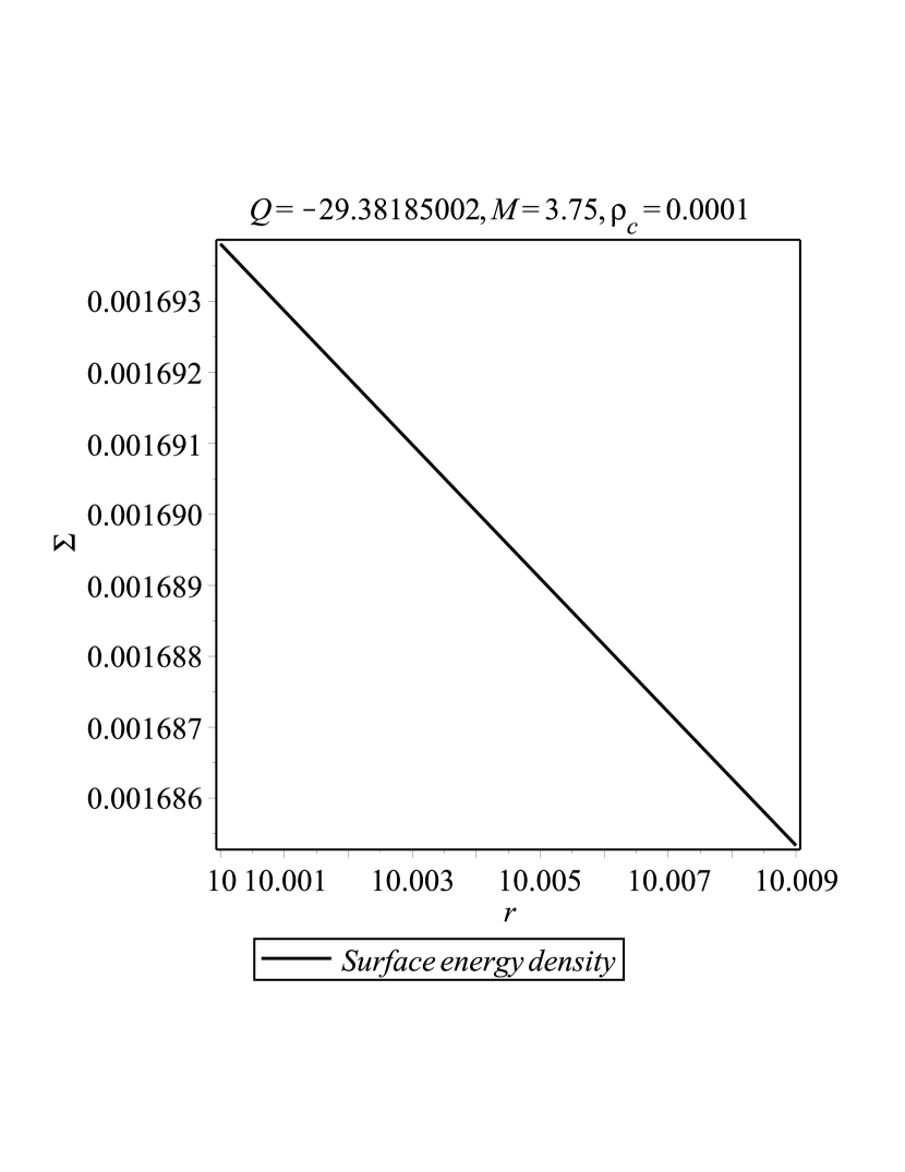
Figure 5: Variation of the surface energy density ($\Sigma$) of the shell with respect to $r$ (km).

Variation of the surface energy density is shown in Fig. 4. We also note that variation of the surface pressure is exactly similar in nature as the surface energy density. There is a discontinuity of the second fundamental form at the junction between the two spacetimes which further implies that there must be a matter component (ultra relativistic fluid) obeying EOS $p=\rho$. This noninteracting matter or the fluid characterizes the existence of the thin shell of the gravastar.

Now one can calculate the mass of the thin shell using the surface energy density of Eq. (69) as

$$m_{s}=4\pi r^{2}\Sigma=R\left[\sqrt{\frac{2}{3}-\frac{4\rho_{c}(2\pi-Q)R^{2}}{9}}-\sqrt{1-\frac{2M}{R}}\right].$$ (71)

With the help of the above equation we can also calculate the total mass of the gravastar in terms of the mass of the thin shell as

$$M=\frac{R}{6}-\frac{m_{s}^{2}}{2R}+m_{s}\sqrt{\frac{2}{3}-\frac{4\rho_{c}R^{2}(2\pi-Q)}{9}}+\frac{2\rho_{c}(2\pi-Q)R^{3}}{9}.$$ (72)

8 Conclusions

In the present work we provide a unique stellar model following the conjecture of Mazur-Mottola [1, 2] under the $f(\mathbb{T},\mathcal{T})$ gravity. The model termed as gravastar by them is assumed to consists of three distinct regions, namely, (i) interior core region, (ii) intermediate shell region, and (iii) exterior vacuum region and each region is governed by specific EOS. With all these specifications we find out a set of exact and singularity-free solutions presenting several interesting and valid properties of the gravastar within in the framework of $f(\mathbb{T},\mathcal{T})$ gravity.

We have noted down several salient aspects of the solution set studying the above mentioned structural form of a gravastar and those can be described below:

(1) Interior region: Using the EOS of (41) along with the conservation equation of Eq. (40) we have found that the matter density as well as the pressure remains constant in the interior. Again using Eqs. (37)- (41) we obtain the metric functions $e^{\lambda(r)}$ and $e^{\nu(r)}$. From these equations it is clear that both the functions are continuous at the origin $r=0$, i.e., free from any central singularity. The variation of the metric function $g_{rr}$ has been shown in Fig. 1.

(2) Intermediate thin shell: Using the thin shell approximation we have solved Einstein’s field equations to obtain the metric functions. The variation of the metric functions $e^{\lambda(r)}$ is shown in Fig. 2. Both the parameters remain finite and positive over the shell. The results provide a physically acceptable solution for the formation of gravastar under $f(\mathbb{T},\mathcal{T})$ gravity.

(3) Proper thickness:The proper thickness or proper length $\ell$ of the shell is found to be gradual increasing in nature from the interior junction to the exterior junction.

(4) Pressure-density: The pressure and density ($p=\rho=0$) of the ultrarelativistic fluid in the shell is plotted with respect to the radial coordinate $r$ in Fig. 3 which shows that the matter density remains positive and increases gradually with the thickness of the shell. This suggests that the shell becomes more denser at the exterior boundary than the interior boundary.

(5) Energy: The energy of the shell is proportional to the radial coordinate $r$ which demands that the energy must be higher at the exterior boundary. The variation of energy is similar as the matter density shown in Fig. 3 and satisfies the requirement that the energy of the shell increases with the radial parameter of the shell.

(6) Entropy: The entropy $S$ within the shell has been obtained in Eq. (60) and the variation is found similar as Fig. 4 which shows that the entropy is gradually increasing with respect to the radial coordinate $r$ indicating a maximum value on the surface of the gravastar that fulfill the physical validity.

(7) Junction condition: We have studied the junction condition for the formation of thin shell between the interior and exterior spacetimes. Following the condition of Darmois and Israel [75, 74] we have studied the surface energy density and surface pressure due to the formation of thin shell. The variation of the surface energy density has been plotted in Figs. 5 and it is observed that the similar behaviour can be obtained forsurface pressure. Thus, both the parameters remain positive, which indicates that the thin shell satisfies the weak and dominant energy conditions. From Eq. (70) it can be claimed for physically acceptable solution we must have $\frac{2M}{r}<1$ and $\rho_{c}(2\pi-Q)R^{2}<\frac{1}{2}$.

Unlike Einstein’s general relativity there are different terms involving the constant $Q$ in the expressions of different physical parameters of the model. This is due to inclusion of the function of torsion scalar $\mathbb{T}$ as well as trace of the energy-momentum tensor $\mathcal{T}$ in the gravitational Lagrangian of the corresponding action. This kind of modification has certainly made the differences between the expressions in both the theories which can be tested by doing a comparative study between this work and that of Rahaman et al. [21] and Ghosh et al. [22] under 4-dimensional background.

References

- [1] P. Mazur, E. Mottola, arXiv:gr-qc/0109035, Report number: LA-UR-01-5067 (2001).
- [2] P. Mazur and E. Mottola, Proc. Natl. Acad. Sci. USA 101, 9545 (2004).
- [3] Y. B. Zel’dovich, Mon. Not. R. Astron. Soc. 160, 1 (1972).
- [4] T. Harko, F. S. N. Lobo, G. Otalora and E. N. Saridakis, J. Cosmol. Astropart. Phys. 12, 021 (2014).
- [5] M. Visser and D. L. Wiltshire, Class. Quantum Gravit. 21, 1135 (2004).
- [6] C. Cattoen, T. Faber and M. Visser, Classical Quantam Gravity 22, 4189 (2005).
- [7] B. M. N. Carter, Classical Quantam Gravity 22, 4551 (2005).
- [8] N. Bilić , G. B. Tupper and R. D. Viollier, J. Cosmol. Astropart. Phys. 02, 013 (2006).
- [9] F. S. N. Lobo, Class. Quantum Gravit. 23, 1525 (2006).
- [10] A. DeBenedictis, D. Horvat, S. Ilijić, S. Kloster and K. S. Viswanathan, Class. Quantum Gravit. 23, 2303 (2006).
- [11] F. S. N. Lobo and A. V. B. Arellano, Class. Quantum Gravit. 24, 1069 (2007).
- [12] D. Horvat and S. Ilijić, Class. Quantum Gravit. 24, 5637 (2007).
- [13] C. B. M. H. Chirenti and L. Rezzolla, Class. Quantum Gravit. 24, 4191 (2007).
- [14] P. Rocha, R. Chan, M. F A. da Silva and A. Wang, J. Cosmol. Astropart. Phys. 11, 010 (2008).
- [15] D. Horvat, S. Ilijić and A. Marunovic, Class. Quantum Gravit. 26, 025003 (2009).
- [16] K. K. Nandi, Y. Z. Zhang, R. G. Cai, and A. Panchenko, Phys. Rev. D 79, 024011 (2009).
- [17] B. V. Turimov, B. J. Ahmedov and A. A. Abdujabbarov, Mod. Phys. Lett. A 24, 733 (2009).
- [18] A. A. Usmani, F. Rahaman, S. Ray, K. K. Nandi, P. K. F. Kuhfittig, Sk. A. Rakib and Z. Hasan, Phys. Lett. B 701, 388 (2011).
- [19] F. S. N. Lobo and R. Garattini, J. High Energy Phys. 12, 065 (2013).
- [20] P. Bhar, Astrophys. Space Sci., 354, 2109 (2014).
- [21] F. Rahaman, S. Chakraborty, S. Ray, A. A. Usmani and S. Islam, Int. J. Theor. Phys. 54, 50 (2015).
- [22] S. Ghosh, F. Rahaman, B. K. Guha and S. Ray, Phys. Lett. B 767, 380 (2017).
- [23] A. G. Riess et al. (SST), Astrophys. J. 607, 665 (2004).
- [24] D. J. Eisenstein et al. (SDSS), Astrophys. J. 633, 560 (2005).
- [25] P. Astier et al. (The SNLS), Astron. Astrophys. 447, 31 (2006).
- [26] D. N. Spergel et al. (WMAP), Astrophys. J. Suppl. 377, 170 (2007).
- [27] C. Möller, Mat-Fys. Skr. Udg. K. Da. 1, 3 (1961).
- [28] C. Pellegrini and J. Plebanski, Mat-Fys. Skr. Udg. K. Da. 2, 1 (1963).
- [29] K. Hayashi and T. Shirafuji, Phys. Rev. D 19, 3524 (1979); 24, 3312(A) (1982).
- [30] H. I. Arcos and J. G. Pereira, Int. J. Mod. Phys. D 13, 2193 (2004).
- [31] A. Unzicker and T. Case, arXiv: physics/0503046.
- [32] R. Aldrovandi and J. G. Pereira, Teleparallel Gravity: An Introduction, Springer, Dordrecht, Netherlands (2013).
- [33] J. W. Maluf, Annalen Phys. 525, 339 (2013).
- [34] Y. Tavakoli, C. Escamilla‐Rivera and J. C. Fabris, Annalen Phys. 529, 1600415 (2017).
- [35] K. F. Dialektopoulos, T. S. Koivisto and S. Capozziello, Eur. Phys. J. C 79, 606 (2019).
- [36] V. Gakis, M. Krššák, J. Levi Said and E. N. Saridakis, arXiv:1908.05741 [gr-qc].
- [37] C. Escamilla-Rivera and J. Levi Said, arXiv:1909.10328 [gr-qc].
- [38] R. Ferraro and F. Fiorini, Phys. Rev. D 75, 084031 (2007).
- [39] G. R. Bengochea and R. Ferraro, Phys. Rev. D 79, 124019 (2009).
- [40] E. V. Linder, Phys. Rev. D 81, 127301 (2010); 82, 109902(E) (2010).
- [41] J.-P. Uzan, Phys. Rev. D 59, 123510 (1999).
- [42] R. de Ritis, A. A. Marino, C. Rubano and P. Scudellaro, Phys. Rev. D 62, 043506 (2000).
- [43] O. Bertolami and P. J. Martins, Phys. Rev. D 61, 064007 (2000).
- [44] V. Faraoni, Phys. Rev. D 62, 023504 (2000).
- [45] L. Amendola, Phys. Lett. B 301, 175 (1993).
- [46] O. Bertolami, C.G. Böhmer, T. Harko and F.S.N. Lobo, Phys. Rev. D 75, 104016 (2007).
- [47] O. Bertolami, F. S. N. Lobo and J. Paramos, Phys. Rev. D 78, 064036 (2008).
- [48] O. Bertolami and J. Paramos, J. Cosmol. Astropart. Phys. 03, 009 (2010).
- [49] T. Harko, Phys. Lett. B 669, 376 (2008).
- [50] T. Harko and F. S. N. Lobo, Eur. Phys. J. C 70, 373 (2010).
- [51] J. Wang and K. Liao, Class. Quantum Gravit. 29, 215016 (2012).
- [52] T. Harko, F. S. N. Lobo and O. Minazzoli, Phys. Rev. D 87, 047501 (2013).
- [53] T. Harko and F. S. N. Lobo, arXiv: 1407.2013.
- [54] T. Harko, F. S. N. Lobo, S. Nojiri and S. D. Odintsov, Phys. Rev. D 84, 024020 (2011).
- [55] A. Das, F. Rahaman, B. K. Guha and S. Ray, Astrophys. Space Sci. 358, 36 (2015).
- [56] A. Das, F. Rahaman, B. K. Guha and S. Ray, Eur. Phys. J. C 76, 654 (2016).
- [57] A. Das, S. Ghosh, B. K. Guha, S. Das, F. Rahaman and S. Ray, Phys. Rev. D 95, 124011 (2017).
- [58] D. Momeni and R. Myrzakulov, Int. J. Geom. Methods Mod. Phys. 11, 1450077 (2014).
- [59] S. B. Nassur, M. J. S. Houndjo, M. E. Rodrigues, A. V. Kpadonou and J. Tossa, Astrophys. Space Sci. 360, 60 (2015).
- [60] I. G. Salako, A. Jawad and S. Chattopadhyay, arXiv:1501.04003 [gr-qc].
- [61] M. G. Ganiou, I. G. Salako, M. J. S. Houndjo and J. Tossa, Astrophys. Space Sci. 361, 57 (2016).
- [62] M. G. Ganiou, I. G. Salako, M. J. S. Houndjo and J. Tossa, Int. J. Theor. Phys. 55, 3954 (2016).
- [63] E. L. B. Junior, M. E. Rodrigues, I. G. Salako and M. J. S. Houndjo, Class. Quantum Gravit. 33, 125006 (2016).
- [64] D. Sáez-Gómez, C. S. Carvalho, F. S. N. Lobo and I. Tereno, Phys. Rev. D 94, 024034 (2016).
- [65] G. Farrugia and J. L. Said, Phys. Rev. D 94, 124004 (2016).
- [66] T. M. Rezaei and A. Amani, Can. J. Phys. 95, 1068 (2017).
- [67] M. Pace and J. L. Said, Eur. Phys. J. C 77, 62 (2017).
- [68] M. Pace and J. L. Said, Eur. Phys. J. C 77, 283 (2017).
- [69] M. G. Ganiou, I. G. Salako, M. J. S. Houndjo and J. Tossa, Int. J. Theor. Phys. 55, 3954 (2016).
- [70] P. S. Wesson, J. Math. Phys (N.Y.) 19, 2283 (1978).
- [71] T. M. Braje and R. W. Romani, Astrophys. J. 580, 1043 (2002).
- [72] L. P. Linares, M. Malheiro and S. Ray, Int. J. Mod. Phys. D 13, 1355 (2004).
- [73] S. Ghosh, S. Ray, F. Rahaman and B. K. Guha, Ann. Phys. 394, 230 (2018)
- [74] W. Israel, Nuo. Cim. 44, 1 (1966); 48, 463(E) (1967).
- [75] G. Darmois, “Mémorial des sciences mathématiques XXV”,
- [76] K. Lanczos, Ann. Phys. (Berlin) 379, 518 (1924).
- [77] N. Sen, Ann. Phys. (Berlin) 378, 365 (1924).
- [78] G. P. Perry and R. B. Mann, Gen. Relativ. Gravit. 24, 305 (1992).
- [79] P. Musgrave and K. Lake, Class. Quantum Gravit. 13, 1885 (1996).