Double Machine Learning based Program Evaluation under Unconfoundedness

Abstract

This paper reviews, applies and extends recently proposed methods based on Double Machine Learning (DML) with a focus on program evaluation under unconfoundedness. DML based methods leverage flexible prediction models to adjust for confounding variables in the estimation of (i) standard average effects, (ii) different forms of heterogeneous effects, and (iii) optimal treatment assignment rules. An evaluation of multiple programs of the Swiss Active Labour Market Policy illustrates how DML based methods enable a comprehensive program evaluation. Motivated by extreme individualised treatment effect estimates of the DR-learner, we propose the normalised DR-learner (NDR-learner) to address this issue. The NDR-learner acknowledges that individualised effect estimates can be stabilised by an individualised normalisation of inverse probability weights.

Keywords: Causal machine learning, conditional average treatment effects, policy learning, individualized treatment rules, multiple treatments, DR-learner

JEL classification: C21

1 Introduction

The adaptation of so-called machine learning to causal inference has been a productive area of methodological research in recent years. The resulting new methods complement the existing econometric toolbox for program evaluation along at least two dimensions <see for recent overviews>Athey2017,Athey2019MachineAbout,Abadie2018EconometricEvaluation. On the one hand, they provide flexible methods to estimate standard average effects. In particular, they provide a data-driven approach to variable and model selection in studies that rely on an unconfoundedness assumption for identification. On the other hand, they enable a more comprehensive evaluation by providing new methods for the flexible estimation of heterogeneous effects and of treatment assignment rules.

This paper considers Double Machine Learning (DML) Chernozhukov, Chetverikov . (2018) as a framework for flexible and comprehensive program evaluation. The DML framework seems attractive because (i) it can be combined with a variety of standard supervised machine learning methods, (ii) it covers average effects for binary <e.g.>Belloni2014InferenceControls,Belloni2017,Chernozhukov2018, multiple <e.g.>Farrell2015 as well as continuous treatments <e.g.>Kennedy2017Non-parametricEffects,Colangelo2019DoubleTreatments,Semenova2021DebiasedFunctions, (iii) it naturally extends to the estimation of heterogeneous treatment effects of different forms like canonical subgroup effects, the best linear prediction of effect heterogeneity, or nonparametric effect heterogeneity <e.g>fan2020EstimationData,Zimmert2019NonparametricConfounding,Foster2019OrthogonalLearning,Oprescu2019OrthogonalInference,Semenova2021DebiasedFunctions,Kennedy2020OptimalEffects,Curth2021NonparametricAlgorithms, and (iv) it can be used to estimate optimal treatment assignment rules <e.g.>Dudik2011DoublyLearning,Athey2021PolicyData,Zhou2018OfflineOptimization. All these DML based methods have favourable statistical properties and allow the use of standard tools like t-tests, OLS, kernel regression, series regression, or supervised machine learning for estimating causal parameters of interest after flexibly adjusting for confounding.

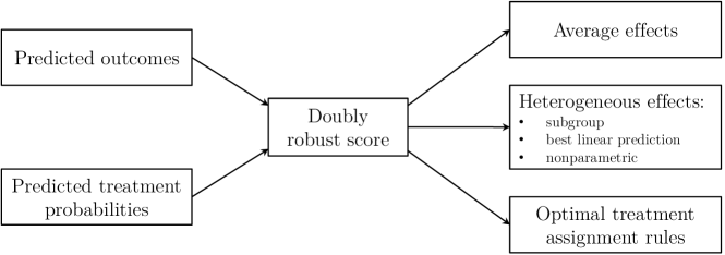
Figure 1: Stylised workflow of Double Machine Learning based program evaluation

This paper starts with a review of DML based methods, then applies these methods in a standard labour economic setting, and comes back to the methods by proposing the normalised DR-learner as a potential fix to a finite sample problem encountered in the application. Thus, it contributes to the steadily growing literature of causal machine learning for program evaluation in three ways. First, the review highlights that methods for different parameters build on the same doubly robust score. The construction of this score might be computationally expensive because it requires the estimation of outcomes and treatment probabilities via machine learning methods. However, once constructed the score can be reused to estimate a variety of interesting parameters. This paper focuses on methods that build on the doubly robust score because they allow to leverage conceptual and computational synergies. The result is a comprehensive pipeline for program evaluation within the same framework as Figure 1 illustrates. This is currently not possible with the variety of more specialised alternatives that integrate machine learning in the estimation of average treatment effects <e.g.>vanderLaan2006TargetedLearning,Athey2018ApproximateDimensions,Avagyan2017HonestEstimation,Tan2020Model-assistedData,Ning2020RobustScore, heterogeneous treatment effects <e.g.>Tian2014,Athey2016,Chernozhukov2017GenericExperiments,Wager2017,Athey2017a,Kunzel2017,Nie2021 and optimal treatment assignment <e.g.>Bansak2018ImprovingAssignment,Kallus2018BalancedLearning.

Second, we use DML based methods to provide a comprehensive and computationally convenient evaluation of four programs of the Swiss Active Labour Market Policy (ALMP) in a standard dataset Lechner . (2020). The evaluation in this paper illustrates the potential of DML based methods for program evaluations under unconfoundedness and provides a potential blueprint for similar analyses. This adds to a small but steadily growing literature that applies causal machine learning to program evaluation in general <e.g.>Bertrand2017,Strittmatter2018WhatEvaluation,Gulyas2019UnderstandingApproach,Knittel2019UsingUse,Davis2020RethinkingJobs,Baiardi2021TheStudies,Farbmacher2021HeterogeneousCognition and to evaluations based on unconfoundedness in particular <e.g>Kreif2019MachineInference,Cockx2020PriorityBelgium,Knaus2020HeterogeneousApproach,Knaus2021ASkills.

Third, we contribute to the methodological literature on the flexible estimation of individualised treatment effects <see for a recent overview>Knaus2021 by proposing the normalised DR-learner (NDR-learner), which builds on the recent DR-learner of Kennedy2020OptimalEffects. The application reveals that the plain DR-learner produces few extreme effect estimates. It turns out that individualised effect estimates can be stabilised by an individualised normalisation of inverse probability weights. Thus, the NDR-learner can be considered as a generalisation of the popular Hajek1971CommentOne normalisation for inverse probability weighting estimators for average effects. The increased stability comes at the price that the NDR-learner limits the class of permissible machine learning methods for effect heterogeneity estimation to methods that form predictions as convex combination of outcomes (e.g. Random Forests).

Overall, we find that DML based methods provide a promising set of methods for program evaluation. The estimated average program effects are in line with the previous literature. We find that computer, vocational and language courses increase employment in the 31 months after programs start, while the effects of job search trainings are mostly negative. The heterogeneity analysis additionally reveals substantial heterogeneities by gender, nationality, previous labour market success and qualification. These are picked up by the estimated optimal assignment rules.

The paper proceeds as follows. Section 2 defines the estimands of interest and their identification under unconfoundedness. Section 3 reviews DML based methods for estimation and introduces the NDR-learner. Section 4 presents the application. Section 5 describes the implementation of the methods. Section 6 reports the results. Section 7 concludes. The Appendix provides additional explanations and results. The R-package causalDML implements the applied estimators. An R notebook replicating the analysis is provided.

2 Estimands of interest

2.1 Definition

We define the estimands of interest in the multiple treatment version of the potential outcomes framework Rubin (1974); Imbens (2000); Lechner (2001). Let $\mathcal{W}=\{0,...,T\}$ denote a set of multiple programs and $D_{i}(w)=\mathds{1}(W_{i}=w)$ a binary variable indicating in which program individual $i$ ($i=1,...,N$) is actually observed. We assume that each individual has a potential outcome $Y_{i}(w)$ for all $w\in\mathcal{W}$. Without loss of generality, the discussion below assumes that higher outcome values are desirable.

The first estimand of interest is the average potential outcome (APO), $\gamma_{w}=E[Y_{i}(w)]$. It answers the question about the average outcome if the whole population was assigned to program $w$. However, the more interesting question is usually to compare different programs $w$ and $w^{\prime}$. To this end, we take the difference of the according individual potential outcomes, $Y_{i}(w)-Y_{i}(w^{\prime})$, and aggregate them to different estimands: First, the average treatment effect (ATE), $\delta_{w,w^{\prime}}=E[Y_{i}(w)-Y_{i}(w^{\prime})]$. Second, the average treatment effect on the treated (ATET), $\theta_{w,w^{\prime}}=E[Y_{i}(w)-Y_{i}(w^{\prime})\mid W_{i}=w]$. Third, the conditional average treatment effect (CATE), $\tau_{w,w^{\prime}}(z)=E[Y_{i}(w)-Y_{i}(w^{\prime})\mid Z_{i}=z]$, where $Z_{i}\in\mathcal{Z}$ is a vector of observed pre-treatment variables.

The different aggregations accommodate the notion that treatment effects might be heterogeneous. ATE represents the average effect in the population, while ATET shows it for the subpopulation that is actually observed in program $w$. Thus, the comparison of ATE and ATET can be informative about the quality of the program assignment mechanism. For example, ATET being larger than ATE indicates that the observed program assignment is better than random.

The ATET is defined by the observed program assignment and thus not subject to the choice of the researcher. In contrast, the conditioning variables $Z_{i}$ of the CATE are specified by the researcher to investigate potentially heterogeneous effects across the groups of individuals that are defined by different values of $Z_{i}$. Such heterogeneous effects can be indicative for underlying mechanisms. Further, CATEs characterise which groups win and which lose by how much by receiving program $w$ instead of $w^{\prime}$.

The different average effects above provide a comprehensive evaluation of programs under the current program assignment policy. In many applications, however, we want to conclude the analysis with a recommendation how the assignment policy could be improved. This can either be done using the evidence on the different average effects defined above or by formally defining the objective of an optimal assignment rule. The latter is pursued by the literature on statistical treatment rules <e.g.>[and references therein]Manski2004StatisticalPopulations,Hirano2009AsymptoticsRules,Stoye2009MinimaxSamples,Stoye2012MinimaxExperiments,Kitagawa2018WhoChoice,Athey2021PolicyData. Here we focus on the case with multiple treatment options as considered by Zhou2018OfflineOptimization.

Let $\pi(Z_{i})$ be a policy that assigns individuals to programs according to their characteristics $Z_{i}$ or, put more formally, the function $\pi(Z_{i})$ maps observable characteristics to a program: $\pi:\mathcal{Z}\rightarrow\mathcal{W}$. In principle, the policy rule can be completely flexible and in the ideal world we would assign each individual to the program with the highest conditional APO, $E[Y_{i}(w)\mid Z_{i}=z]$. However, in many cases we want to restrict the set of candidate policy rules denoted by $\Pi$ to be interpretable for the communication with decision makers or to incorporate costs or fairness constraints. Each of these candidate policy rules has a policy value function denoted by $Q(\pi)=E[Y_{i}(\pi(Z_{i}))]=E\left[\sum_{w}\mathds{1}(\pi(Z_{i})=w)Y_{i}(w)\right]$. $Q(\pi)$ quantifies the average population outcome if policy rule $\pi$ would be used to assign programs. The estimand of interest is then the optimal policy rule $\pi^{*}$ with the highest value function for the set of candidate policy rules, or formally $\pi^{*}=\operatorname*{\arg\max}_{\pi\in\Pi}Q(\pi)$.

2.2 Identification

The previous section defined the estimands of interest in terms of potential outcomes. However, each individual is only observed in one program. Thus, only one potential outcome per individual is observable and the other potential outcomes remain latent. This is the fundamental problem of causal inference Holland (1986) and we need further assumptions to identify the estimands of interest. In this paper, we consider the unconfoundedness assumption that assumes access to a vector of pre-treatment variables $X_{i}\in\mathcal{X}$ containing $Z_{i}$ such that the following standard assumptions hold <e.g.>Imbens2015CausalSciences:

Assumption 1

  

(a) Unconfoundedness: $Y_{i}(w)\mathrel{\text{\scalebox{1.07}{$\perp\mkern-10.0mu\perp$}}}W_{i}\mid X_{i}=x$, $\forall$ $w\in\mathcal{W}$, and $x\in\mathcal{X}$.

(b) Common support: $0<P[W_{i}=w\mid X_{i}=x]\equiv e_{w}(x)$, $\forall$ $w\in\mathcal{W}$ and $x\in\mathcal{X}$.

(c) Stable Unit Treatment Value Assumption (SUTVA): $Y_{i}=Y_{i}(W_{i})$.

The unconfoundedness assumption requires that $X_{i}$ contains all confounding variables that jointly affect program assignment and the outcome. Common support states that it must be possible to observe each individual in all programs. SUTVA rules out interference. These assumptions allow the identification of the average potential outcome (APO) conditional on confounders in three common ways:

$$E[Y_{i}(w)\mid X_{i}=x] =E\left[Y_{i}\mid W_{i}=w,X_{i}=x\right]\equiv\mu(w,x)$$ (1)

$$=E\left[\dfrac{D_{i}(w)Y_{i}}{e_{w}(x)}\middle|X_{i}=x\right]$$ (2)

$$=E\biggl{[}\underbrace{\mu(w,x)+\dfrac{D_{i}(w)(Y_{i}-\mu(w,x))}{e_{w}(x)}}_{\begin{subarray}{c}\equiv\Gamma(w,x)\end{subarray}}\biggm{|}X_{i}=x\biggr{]}$$ (3)

Equation 1 shows that the conditional APO is identified as a conditional expectation of the observed outcome. Equation 2 shows that it is identified by reweighting the observed outcome with the inverse treatment probability. Finally, Equation 3 adds the reweighted outcome residual to the conditional outcome representation of Equation 1. This seems redundant because we can check that the reweighted residual has expectation zero under unconfoundedness. However, this identification result is doubly robust in the sense that it still holds if we replace either $\mu(w,x)$ or $e_{w}(x)$ in Equation 3 by arbitrary functions of $x$. This doubly robust structure plays a crucial role for the estimation procedures that we discuss in the next section.

From an identification perspective, $\Gamma(w,x)$ defined in Equation 3 suffices to identify all estimands of interest stated in the previous subsection:

• APO: $\gamma_{w}=E[Y_{i}(w)]=E[\Gamma(w,X_{i})]$

• ATE: $\delta_{w,w^{\prime}}=E[Y_{i}(w)-Y_{i}(w^{\prime})]=E[\Gamma(w,X_{i})-\Gamma(w^{\prime},X_{i})]$

• ATET: $\theta_{w,w^{\prime}}=E[Y_{i}(w)-Y_{i}(w^{\prime})\mid W_{i}=w]=E[\Gamma(w,X_{i})-\Gamma(w^{\prime},X_{i})\mid W_{i}=w]$

• CATE: $\tau_{w,w^{\prime}}(z)=E[Y_{i}(w)-Y_{i}(w^{\prime})\mid Z_{i}=z]=E[\Gamma(w,X_{i})-\Gamma(w^{\prime},X_{i})\mid Z_{i}=z]$

• Policy value: $Q(\pi)=E[Y_{i}(\pi(Z_{i}))]=E[\sum_{w}\mathds{1}(\pi(Z_{i})=w)\Gamma(w,X_{i})]$

• Optimal policy: $\pi^{*}=\operatorname*{\arg\max}_{\pi\in\Pi}Q(\pi)=\operatorname*{\arg\max}_{\pi\in\Pi}E[\sum_{w}\mathds{1}(\pi(Z_{i})=w)\Gamma(w,X_{i})]$

3 Estimation based on Double Machine Learning

3.1 The doubly robust scores

All Double Machine Learning (DML) based estimators for the estimands of interest build on the doubly robust scores of Robins1994,Robins1995AnalysisData and their Augmented Inverse Probability Weighting (AIPW) estimator in particular. In the following, large Greek letters denote the scores corresponding to the small Greek letters used to define the estimands in Section 2.1.

The construction of the doubly robust scores requires the input of so-called nuisance parameters that are usually of secondary interest and considered as tool to eventually obtain the parameters of interest. In our case, the two nuisance parameters are ${\mu(w,x)=E[Y_{i}\mid W_{i}=w,X_{i}=x]}$ and $e_{w}(x)=P[W_{i}=w\mid X_{i}=x]$ for all $w$. $\mu(w,x)$ is the conditional outcome mean for the subgroup observed in program $w$. $e_{w}(x)$ is the conditional probability to be observed in program $w$, also known as the propensity score. Usually these functions are unknown and need to be estimated. Following Chernozhukov2018 they are estimated based on $K$-fold cross-fitting: (i) randomly divide the sample in $K$ folds of similar size, (ii) leave out fold $k$ and estimate models for the nuisance parameters in the remaining $K-1$ folds, (iii) use these models to predict $\hat{\mu}^{-k}(w,x)$ and $\hat{e}^{-k}_{w}(x)$ in the left out fold $k$, and (iv) repeat (i) to (iii) such that each fold is left out once. This procedure avoids overfitting in the sense that no observation is used to predict its own nuisance parameters. To avoid notational clutter, we ignore the dependence on the specific fold in the following notation and refer to the cross-fitted nuisance parameters as $\hat{\mu}(w,x)$ and $\hat{e}_{w}(x)$.

The main building block of the following estimators is the doubly robust score of the APO, which replaces the true nuisance parameters in Equation 3 by their cross-fitted predictions:

$$\hat{\Gamma}_{i,w}=\hat{\mu}(w,X_{i})+\dfrac{D_{i}(w)(Y_{i}-\hat{\mu}(w,X_{i}))}{\hat{e}_{w}(X_{i})}.$$ (4)

The ATE score for the comparison of treatment $w$ and $w^{\prime}$ is then constructed as the difference of the respective APO scores:

$$\hat{\Delta}_{i,w,w^{\prime}}=\hat{\Gamma}_{i,w}-\hat{\Gamma}_{i,w^{\prime}}$$ (5)

The only estimator we consider that uses the same nuisance parameter but plugs them into a different score is the ATET estimator. Although the identification result with the doubly robust APO score in the previous section holds, it is not doubly robust. However, the doubly robust score for the ATET exists and is defined as

$$\hat{\Theta}_{i,w,w^{\prime}}=\dfrac{D_{i}(w)(Y_{i}-\hat{\mu}(w^{\prime},X_{i}))}{\hat{e}_{w}}-\dfrac{D_{i}(w^{\prime})\hat{e}_{w}(X_{i})(Y_{i}-\hat{\mu}(w^{\prime},X_{i}))}{\hat{e}_{w}\hat{e}_{w^{\prime}}(X_{i})},$$ (6)

where $\hat{e}_{w}=N_{w}/N$ is the unconditional treatment probability with $N_{w}$ counting the number of individuals observed in program $w$ <see also, e.g.>Farrell2015.

3.2 Average potential outcomes and treatment effects

The estimation of the APOs, ATEs and ATETs boils down to taking the means of the previously defined doubly robust scores. For statistical inference, we can rely on standard one-sample t-tests. Thus, the score’s mean and the variance of this mean are the point and the variance estimate of the respective estimand of interest:

• APO: $\hat{\mu}_{w}=N^{-1}\sum_{i}\hat{\Gamma}_{i,w}$ and $\hat{\sigma}^{2}_{\mu_{w}}=N^{-1}\sum_{i}(\hat{\Gamma}_{i,w}-\hat{\mu}_{w})^{2}$

• ATE: $\hat{\delta}_{w,w^{\prime}}=N^{-1}\sum_{i}\hat{\Delta}_{i,w,w^{\prime}}$ and $\hat{\sigma}^{2}_{\delta_{w,w^{\prime}}}=N^{-1}\sum_{i}(\hat{\Delta}_{i,w,w^{\prime}}-\hat{\delta}_{w,w^{\prime}})^{2}$

• ATET: $\hat{\theta}_{w,w^{\prime}}=N^{-1}\sum_{i}\hat{\Theta}_{i,w,w^{\prime}}$ and $\hat{\sigma}^{2}_{\theta_{w,w^{\prime}}}=N^{-1}\sum_{i}(\hat{\Theta}_{i,w,w^{\prime}}-\hat{\theta}_{w,w^{\prime}})^{2}$

Note that the estimated variances require no adjustment for the fact that we have estimated the nuisance parameters in a first step. The resulting estimators are consistent, asymptotically normal and semiparametrically efficient under the main assumption that the estimators of the cross-fitted nuisance parameters are consistent and converge sufficiently fast Belloni . (2014); Farrell (2015); Belloni . (2017); Chernozhukov, Chetverikov . (2018). In particular, the product of the convergence rates of the outcome and propensity score estimators must be faster than $n^{1/2}$. This allows to apply machine learning to estimate the nuisance parameters. Flexible machine learning estimators converge usually slower than the parametric rate $n^{1/2}$ but several are known to be able to achieve $n^{1/4}$ and faster, which would be sufficient if both nuisance parameter estimators achieve it.

It is well known that estimators using doubly robust scores and parametric models for the nuisance parameters are doubly robust in the sense that they remain consistent if one of the parametric models is misspecified <see, e.g.>Glynn2009AnEstimator. The difference of the DML version is that it exploits what Smucler2019AContrasts call ’rate double robustness’. This robustness allows to estimate the parameters of interest at the parametric rate $n^{1/2}$ even if the nuisance parameters are estimated at slower rates using machine learning methods that do not require the specification of an actual parametric model.

The rate double robustness is the consequence of the so-called Neyman orthogonality of the doubly robust score. Neyman orthogonality is at the heart of the general DML framework of Chernozhukov, Chetverikov . (2018). Scores with this orthogonality are immune against small errors in the estimation of nuisance parameters and thus allow them to be estimated via machine learning. Appendix A.2 revisits what this means in formal terms.

3.3 Conditional average treatment effects

3.3.1 DR-learner

We can reuse the ATE score of Equation 5 to estimate conditional effects. The so-called DR-learner was introduced for binary treatments but directly translates also to multiple treatments settings. It exploits that the conditional expectation of the score with known nuisance parameters equals CATE: $\tau_{w,w^{\prime}}(z)=E[\Delta_{i,w,w^{\prime}}\mid Z_{i}=z]$. Thus, a natural way to estimate CATEs is to use the score with estimated nuisance parameters, $\hat{\Delta}_{i,w,w^{\prime}}$, as pseudo-outcome in a general regression framework:

$$\hat{\tau}^{dr}(Z_{i})=\operatorname*{\arg\min}_{\tau}\sum_{i=1}^{N}\left(\hat{\Delta}_{i,w,w^{\prime}}-\tau(Z_{i})\right)^{2}$$ (7)

From a conceptual and estimation perspective it is instructive to distinguish two special cases of CATEs at this point <see also>Knaus2021: (i) Group average treatment effects (GATE) provide the average effects for pre-specified, usually low-dimensional, groups. This covers standard subgroup analysis comparing, e.g., effects of men and women, or heterogeneity along pre-specified continuous variables like age. (ii) Individualised average treatment effects (IATEs) aim for the most detailed effect heterogeneity considering all confounders as heterogeneity variables, i.e. $Z_{i}=X_{i}$ and thus $IATE(x)=\tau_{w,w^{\prime}}(x)=E[Y_{i}(w)-Y_{i}(w^{\prime})\mid X_{i}=x]$.

OLS, series or kernel regressions of the pseudo-outcome on low-dimensional heterogeneity variables estimate GATEs. The outputs of such regressions can be interpreted in the standard way. The only difference is that instead of modelling the level of an outcome, they now model the level of a causal effect. Most importantly standard statistical inference applies as is shown for OLS and series regression by Semenova2021DebiasedFunctions as well as for kernel regression by fan2020EstimationData and Zimmert2019NonparametricConfounding. Similar to the discussion in the previous section, the Neyman orthogonality of $\Delta_{i,w,w^{\prime}}$ allows to ignore that nuisance parameters are estimated with flexible methods potentially converging slower than $n^{1/2}$ when calculating standard errors. The details about the required convergence rates are discussed in the referenced papers.

IATEs may be estimated using the pseudo-outcome in supervised machine learning regressions with the full set of confounders as predictors. As discussed by Chernozhukov2017GenericExperiments statistical inference is not yet well understood for low-dimensional $Z_{i}$ and even harder for high-dimensional $Z_{i}$ when machine learning is used to solve Equation 7. However, Kennedy2020OptimalEffects shows that the doubly robust structure of the ATE score results in favourable bounds on the mean squared error for the estimated IATEs that would not be attainable by outcome regression or IPW based methods alone.

We consider two variants of the DR-learner for IATEs. First, we reuse the pseudo-outcome in one supervised machine learning regression to estimate IATEs in-sample. This full sample procedure is computationally convenient but prone to overfitting. Thus, the second variant produces out-of-sample IATE predictions for each individual in the sample. Following Algorithm 1 of Kennedy2020OptimalEffects, this requires a four-fold cross-fitting scheme that is detailed in Algorithm 2 of Appendix B. The computational downside of this procedure is that we cannot reuse the same nuisance parameter predictions as for the average estimator and need to estimate them for the IATE only. However, the results below suggest that this computational effort is important to avoid severe overfitting.

3.3.2 Normalised DR-learner

Note that the point estimates of the plain DR-learner can be expressed as $\hat{\tau}^{dr}(z)=\sum_{i=1}^{N}\alpha_{i}\hat{\Delta}_{i,w,w^{\prime}}$ if the weight $\alpha_{i}$ that each observation receives can be calculated. For example, the ATE estimator as special case of the DR-learner with $Z_{i}$ being a constant uses $\alpha_{i}=1/N$, the least squares regression uses $\alpha_{i}=z(\bm{Z^{\prime}}\bm{Z})^{-1}\bm{Z^{\prime}}$ with $\bm{Z}$ being the stacked covariate matrix, and the kernel regression uses $\alpha_{i}=\frac{\mathcal{K}_{h}\left(Z_{i}-z\right)}{\sum_{i=1}^{N}\mathcal{K}_{h}\left(Z_{i}-z\right)}$ with $\mathcal{K}_{h}$ representing a proper kernel function. The class of estimators with a known weighted representation is called linear smoothers <see e.g.>Buja1989LinearModels. Popular machine learners like tree-based methods (regression trees, Random Forests or boosted trees), Ridge or any method that runs OLS after variable selection like Post-Lasso Belloni  Chernozhukov (2013) have this structure. Also for these methods we know the weight $\alpha_{i}(x)$ that each observation receives in predicting the (pseudo-)outcome at $x$. These weights usually sum up to one, i.e. $\sum_{i=1}^{N}\alpha_{i}(x)=1$. Using such outcome weighting predictors in the final step allows to express the DR-learner estimated IATE as

$$\hat{\tau}_{w,w^{\prime}}^{drl}(x) =\sum_{i=1}^{N}\alpha_{i}(x)\hat{\Delta}_{i,w,w^{\prime}}$$

$$=\sum_{i=1}^{N}\alpha_{i}(x)[\hat{\mu}(w,X_{i})-\hat{\mu}(w^{\prime},X_{i})]$$

$$\quad+\sum_{i=1}^{N}\underbrace{\dfrac{\alpha_{i}(x)D_{i}(w)}{\hat{e}_{w}(X_{i})}}_{\lambda^{w}_{i}(x)}\tilde{Y_{i}}(w,X_{i})-\sum_{i=1}^{N}\underbrace{\dfrac{\alpha_{i}(x)D_{i}(w^{\prime})}{\hat{e}_{w^{\prime}}(X_{i})}}_{\lambda^{w^{\prime}}_{i}(x)}\tilde{Y_{i}}(w^{\prime},X_{i}),$$ (8)

where $\tilde{Y_{i}}(w,X_{i})=Y_{i}-\hat{\mu}(w,X_{i})$ denotes the outcome residual.

The DR-learner shares the problem of all estimators that involve reweighting by the inverse of the propensity score. In finite samples, ${\lambda^{w}_{i}}(x)$ and ${\lambda^{w^{\prime}}_{i}}(x)$ usually do not sum to one, i.e. $\sum_{i=1}^{N}{\lambda^{w}_{i}}(x)\neq 1$ and $\sum_{i=1}^{N}{\lambda^{w^{\prime}}_{i}}(x)\neq 1$. This is especially problematic if it sums to something much greater than one. In this case the weighted residuals receive much more weight than the outcome regressions. This might result in implausibly large effect estimates that even could fall outside of the possible bounds of a given outcome variable Kang  Schafer (2007); Robins . (2007).

For average effects the Hajek1971CommentOne normalisation is recommended to stabilise estimators using inverse probability weights <e.g.>Imbens2004NonparametricReview,Lunceford2004StratificationStudy,Robins2007Comment:Variable,busso2014new. However, Equation 8 highlights that the inverse probability weights become $x$-specific and such a one time normalisation that targets the average effect does not solve the problem for the individualised effect. This can be problematic as finite sample imbalances are more likely to occur on the individualised level. Thus, we propose the normalised DR-learner (NDR-learner) as a stabilised complement to the DR-learner.

The NDR-learner normalises the weighted residuals by the sum of weights:

$$\hat{\tau}_{w,w^{\prime}}^{ndrl}(x)= \sum_{i=1}^{N}\alpha_{i}(x)[\hat{\mu}(w,X_{i})-\hat{\mu}(w^{\prime},X_{i})]$$

$$+\left(\sum_{i=1}^{N}\lambda^{w}_{i}(x)\right)^{-1}\sum_{i=1}^{N}\lambda^{w}_{i}(x)\tilde{Y_{i}}(w,X_{i})-\left(\sum_{i=1}^{N}\lambda^{w^{\prime}}_{i}(x)\right)^{-1}\sum_{i=1}^{N}\lambda^{w^{\prime}}_{i}(x)\tilde{Y_{i}}(w^{\prime},X_{i})$$ (9)

This ensures that the weights of the residuals sum up to one under the condition that weights $\alpha_{i}(x)$ are non-negative. Thus, methods like Ridge or Post-Lasso with potentially negative weights might not be applicable.

The NDR-learner is more demanding from a computational point of view because it requires to calculate the weights $\alpha_{i}(x)$ and the normalisation for each $x$ of interest (Algorithm 2 in Appendix B provides the details of the implementation). However, the application below shows that the normalisation deals well with the cases where outcome residuals receive high weights leading to implausibly large effect estimates. Thus, the NDR-learner is an interesting alternative to the DR-learner if effect sizes become suspicious.

3.4 Optimal treatment assignment

The APO score of Section 3.1 can also be reused to estimate optimal treatment assignment. To this end, note that the value function of any policy rule $\pi(Z_{i})$ can be estimated as

$$\hat{Q}(\pi)=N^{-1}\sum_{i=1}^{N}\sum_{w=0}^{T}\mathds{1}(\pi(Z_{i})=w)\hat{\Gamma}_{i,w}.$$

This means each individual contributes the score of the treatment that she is assigned to under this policy rule. However, we are not necessarily interested in the value function of some policy rule, but want to estimate the optimal policy rule that maximises this value function, $\hat{\pi}^{*}=\operatorname*{\arg\max}_{\pi\in\Pi}\hat{Q}(\pi)$. This requires to search over all candidate policy rules to find the optimum as there exists no closed form solution.

Example: Consider the case where $Z_{i}$ is a binary covariate and $W_{i}$ is a binary treatment. We have four different policy rules: treat nobody ($\pi^{1}$), treat only those with $Z_{i}=1$ ($\pi^{2}$), treat only those with $Z_{i}=0$ ($\pi^{3}$), or treat everybody ($\pi^{4}$). We illustrate this using two representative observations, $i=1$ with $Z_{1}=0$, and $i=2$ with $Z_{2}=1$ in Table 1. The columns three to six show the assignments under the four potential assignment rules. For example, the first observation receives no treatment under policy rules $\pi^{1}$ and $\pi^{2}$, but is treated under policy rules $\pi^{3}$ and $\pi^{4}$. To find the optimal rule, we compare the means of the APO scores in the last four columns and pick the policy rule that corresponds to the largest mean. The number of policy values to compare increases dramatically in settings with multiple treatments and $Z_{i}$ being a vector of potentially non-binary variables.

Table 1: Example of DML based optimal treatment assignment

$i$	$Z_{i}$	$\pi^{1}$	$\pi^{2}$	$\pi^{3}$	$\pi^{4}$	$\hat{Q}(\pi^{1})$	$\hat{Q}(\pi^{2})$	$\hat{Q}(\pi^{3})$	$\hat{Q}(\pi^{4})$
1	0	0	0	1	1	$\hat{\Gamma}_{1,0}$	$\hat{\Gamma}_{1,0}$	$\hat{\Gamma}_{1,1}$	$\hat{\Gamma}_{1,1}$
2	1	0	1	0	1	$\hat{\Gamma}_{2,0}$	$\hat{\Gamma}_{2,1}$	$\hat{\Gamma}_{2,0}$	$\hat{\Gamma}_{2,1}$
⋮	⋮	⋮	⋮	⋮	⋮	⋮	⋮	⋮	⋮

We expect that the estimated policy in finite samples and with estimated nuisance parameters does not coincide with the true optimal policy rule. This is conceptualised as the ’regret’ defined as the difference between the true and the estimated optimal value function, $R(\hat{\pi}^{*})=Q(\pi^{*})-Q(\hat{\pi}^{*})$.

Zhou2018OfflineOptimization show that the DML based procedure minimises the maximum regret asymptotically under two main conditions: First, the same convergence conditions for the nuisance parameters that are required for ATE estimation (the product of the nuisance parameter convergence rates achieves $n^{1/2}$). Second, the set of candidate policy rules $\Pi$ is not too complex. In particular, Zhou2018OfflineOptimization show that decision trees with fixed depth are a suitable class of policy rules. Again the double robustness of the used scores results in statistical guarantees that are not achievable for methods based on outcome regressions or IPW alone.

4 Application: Swiss Active Labour Market Policy

We use a standard observational dataset of Swiss Active Labour Market Policy (ALMP) that is already basis of previous studies Huber . (2017); Lechner (2018); Knaus . (2020) to estimate the effect of different programs on employment. In particular, we start with the sample of 100,120 unemployed individuals of Huber2017 that consists of 24 to 55 year old individuals registered unemployed in 2003. We consider non-participants and participants of four different program types: job search, vocational training, computer programs and language courses. As the assignment policies differ substantially across the three language regions, we focus only on individuals living in the German speaking part and remove those in the French and Italian speaking part to avoid common support problems.

We evaluate the first program participation within the first six months after the begin of the unemployment spell. One problem of this definition is that non-participants comprise people that quickly come back into employment before they would be assigned to a training program. This could result in an overly optimistic evaluation of non-participation. We follow lechner1999earnings and lechner2007value and assign pseudo program starting points to the non-participants and keep only those who are still unemployed at this point. This results in a final sample size of 62,497 observations.

[t]

Table 2: Descriptive statistics of selected variables by program type

	No program	Job search	Vocational	Computer	Language
	(1)	(2)	(3)	(4)	(5)
No. of observations	47,620	11,610	858	905	1504
Outcome: months employed of 31	14.7	14.4	18.4	19.2	13.5
Female (binary)	0.44	0.44	0.33	0.60	0.55
Age	36.6	37.3	37.5	39.1	35.3
Foreigner (binary)	0.36	0.33	0.30	0.21	0.66
Employability	1.93	1.98	1.93	1.97	1.85
Past income in CHF 10,000	4.25	4.67	4.87	4.32	3.73

• Note: Employability is an ordered variable with one indicating low employability, two medium employability and three high employability. The exchange rate USD/CHF was roughly 1.3 at that time. The full set of variables is reported in Table C.1.

The outcome of interest is the cumulated number of months in employment in the 31 months after program start, which is the maximum available time span in the dataset. Row one of Table 2 provides the number of observations in each group. Roughly 75% participate in no program. By far the largest program is the job search program, which is also called basic program. The more specific programs are much smaller with roughly 1000 observations each. Row two shows that the average outcomes substantially differ by different groups. However, it is not clear whether this is only due to selection effects because the observable characteristics are not comparable across groups, as the remaining rows show. Especially the share of females, the share of foreigners and past income differ quite substantially across programs. The confounders comprise 45 variables and are reported in Table C.1 of Appendix C. They consist of socio-economic characteristics of the unemployed individuals, caseworker characteristics, information about the assignment process, information about the previous job, and regional economic indicators.

5 Implementation

The nuisance parameters are estimated via Random Forest Breiman (2001) using the implementation with honest splitting in the grf R-package Athey . (2019) and 5-fold cross-fitting. The tuning parameters in each regression are selected by out-of-bag validation. All regressions apply the full set of confounders. We run the outcome regressions for each treatment group separately to obtain $\hat{\mu}(w,x)$. Also the propensity scores are separately estimated for each treatment using a treatment indicator as outcome in the random forest. The propensity scores are then normalised to sum to one within an individual.

We estimate CATEs at different granularity. First, we investigate GATEs for subgroups by gender, foreigners and three categories of employability. These are regularly used in the program evaluation literature and usually investigated by re-estimating everything in the subgroups. However, it can be performed at very low computational costs after DML for average effects using only a standard OLS regression with the pseudo-outcome as described in Section 3.3.1 and using dummy variables for all groups but the reference group as covariates. Second, we estimate kernel regression and spline regression GATEs for the continuous variables age and past income based on the R-packages np Hayfield  Racine (2008) and crs Racine  Nie (2021), respectively. The kernel regressions apply a second-order Gaussian kernel function and use 0.9 of the cross-validated bandwidth for undersmoothing as suggested by Zimmert2019NonparametricConfounding. The spline regressions use B-splines with cross-validated degree and number of knots. Third, we specify an OLS regression in which all the five previously used variables enter linearly. Finally, we go beyond the handpicked variables and estimate the IATEs using all 45 confounders in the DR-learner and the NDR-learner. Both are implemented with the honest Random Forest because the grf package allows to extract the prediction weights $\alpha_{i}(x)$ required for the NDR-learner. We apply both variants described in Section 3.3.1. Once we estimate the IATE for each observation using DR- and NDR-learner in the full sample and once we predict them out-of-sample. For the latter, Appendix B provides a detailed description of the underlying DR- and NDR-learner algorithms.

Table 3: Steps of implementation

Step	Input	Operation	Output
1.	$W_{i}$, $X_{i}$	Predict treatment probabilities	$\hat{e}_{w}(x)$
2.	$Y_{i}$, $W_{i}$, $X_{i}$	Predict treatment specific outcomes	$\hat{\mu}(w,x)$
3.	$Y_{i}$, $W_{i}$, $\hat{e}_{w}(x)$, $\hat{\mu}(w,x)$	Plug into Equation 4	$\hat{\Gamma}_{i,w}$
4.	$\hat{\Gamma}_{i,w}$	Mean, one-sample t-test	APOs
5.	$\hat{\Gamma}_{i,w}$	Take difference	$\hat{\Delta}_{i,w,w^{\prime}}$
6.	$\hat{\Delta}_{i,w,w^{\prime}}$	Mean, one-sample t-test	ATEs
7.	$\hat{\Delta}_{i,w,w^{\prime}}$, $Z_{i}$	OLS/Kernel/Series regression	GATEs
8.	$\hat{\Delta}_{i,w,w^{\prime}}$, $X_{i}$	Supervised Machine Learning	IATEs
9.	$\hat{\Gamma}_{i,w}$, $Z_{i}$	Optimal decision tree	Optimal treament rule

The optimal treatment assignment rule is estimated as decision trees of depth one, two and three. We follow Algorithm 2 for exact tree-search of Zhou2018OfflineOptimization that is implemented in the policytree R-package Sverdrup . (2020). We estimate the trees first with the five handpicked variables. However, these variables include gender and foreigner status that might be too sensitive to include in practice. Thus, we investigate another set of 16 variables that includes only the objective measures of education and labour market history of the unemployed persons that would be available for recommendations from the administrative records.

Table 3 summarises all required implementation steps. It highlights that a comprehensive DML based program evaluation can be run with few lines of code in any statistical software program that is capable of the operations in the third column. Thus, researchers can build their customised analyses in a modular fashion based on established code. Alternatively, the R-package causalDML already implements the required steps as showcased in the replication notebook accompanying this paper. Most importantly the package provides a fast implementation of the individualised normalisation required for the NDR-learner in C++.

6 Results

6.1 Average effects

We focus here on the effect estimates and discuss the nuisance parameters in Appendix C.2. Throughout this section, we compare the four programs to non-participation. Recall that the outcome of interest is the cumulated number of months employed in the 31 months after program start. Figure 2(a) depicts ATE and ATET estimates and shows substantial differences in the effectiveness of programs. The job search program decreases the months in employment on average by about one month. In contrast, other programs that teach hard skills show substantial improvements with roughly three additional months in employment on average.

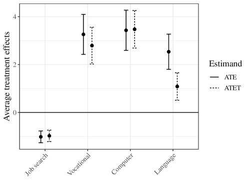
Figure 2: Average treatment effects of participation vs. non-participation

(a) Note: The figure shows the point estimates of the average treatment effects of participating in the program labeled on the x-axis vs. non-participation and their 95% confidence intervals. Numeric results in Panels B and C of Table C.5 of Appendix C.

Comparing ATE and ATET shows no big differences for most programs. This suggests that there is either no effect heterogeneity correlated with observables or that the assignment does not take advantage of this heterogeneity. We would expect to see ATETs being higher than ATEs if program assignment is well targeted. However, we find only evidence for the opposite as the actual participants of a language course show a 1.5 months lower treatment effect compared to the population. This difference suggests that there is substantial effect heterogeneity to uncover and the potential to improve treatment assignment.

6.2 Heterogeneous effects

6.2.1 Subgroup GATEs

This subsection studies effect heterogeneity at different granularity. We start by estimating group average treatment effects (GATEs) for discrete subgroups. Panel A of Table 4 shows the result of an OLS regression with a female dummy as covariate, $\hat{\Delta}_{i,w,w^{\prime}}=\beta_{0}+\beta_{1}female_{i}+error_{i}$. The constant ($\beta_{0}$) provides the GATE for the reference group men and the female coefficient ($\beta_{1}$) describes how much the GATE differs for women. The results show substantial gender differences in the effectiveness of programs. Women significantly suffer less or profit more from job search and computer program participation. This gender gap in the effectiveness of ALMPs is also well-documented in the literature Crépon  van den Berg (2016); Card . (2018). In contrast to this, we find that women profit on average significantly less from language courses than men.

Table 4: Group average treatment effects

	Job search	Vocational	Computer	Language
	(1)	(2)	(3)	(4)
Panel A:
Constant	-1.29∗∗∗	3.82∗∗∗	2.33∗∗∗	3.40∗∗∗
	(0.17)	(0.55)	(0.60)	(0.46)
Female	0.60∗∗	-1.27	2.49∗∗∗	-1.97∗∗
	(0.25)	(0.87)	(0.85)	(0.77)
Panel B:
Constant	-1.27∗∗∗	2.48∗∗∗	3.75∗∗∗	3.56∗∗∗
	(0.16)	(0.53)	(0.50)	(0.52)
Foreigner	0.70∗∗∗	2.17∗∗	-0.88	-2.84∗∗∗
	(0.26)	(0.90)	(0.93)	(0.72)
Panel C:
Constant	-0.18	5.48∗∗∗	5.76∗∗∗	2.61∗∗∗
	(0.33)	(1.04)	(1.10)	(0.85)
Medium employability	-0.93∗∗∗	-2.41∗∗	-2.67∗∗	-0.18
	(0.36)	(1.16)	(1.20)	(0.96)
High employability	-1.50∗∗∗	-4.42∗∗∗	-3.59∗∗	0.59
	(0.50)	(1.52)	(1.69)	(1.48)
F-statistic	5.04∗∗∗	4.31∗∗	2.96∗	0.18

• Note: This table shows OLS coefficients and their heteroscedasticity robust standard errors (in parentheses) of regressions run with the pseudo-outcome defined as described in Section 3.3. ^∗p$<$0.1; ^∗∗p$<$0.05; ^∗∗∗p$<$0.01

Panel B replaces the female dummy in the regression by a foreigner dummy. Strikingly, Swiss citizens as reference group show a big positive effect for participating in language courses but the effect disappears for foreigners. After adding the coefficient for foreigners to the constant, the foreigners’ GATE is only 0.72 ($3.56-2.84$, standard error: 0.69). A crucial information to better understand this finding would be to know which languages they learn. However, this information is unfortunately not available in the dataset.

Panel C shows the results of a similar regression but now with two dummies indicating medium and high employability such that low employability becomes the reference group. The F-statistic in the last line tests the joint significance of the two dummies. It is statistically significant at least at the 10%-level for the programs in the first three columns. They all show a common gradient that individuals with low employability benefit substantially more or at least suffer less from program participation.

6.2.2 Nonparametric GATEs for continuous heterogeneity variables

Figure 3: Effect heterogeneity regarding past income

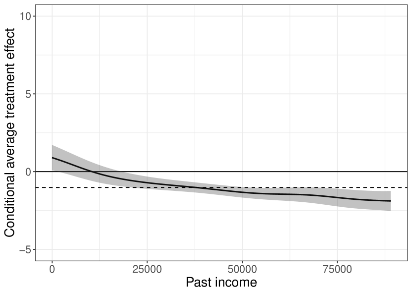
(a) Job search (Kernel)

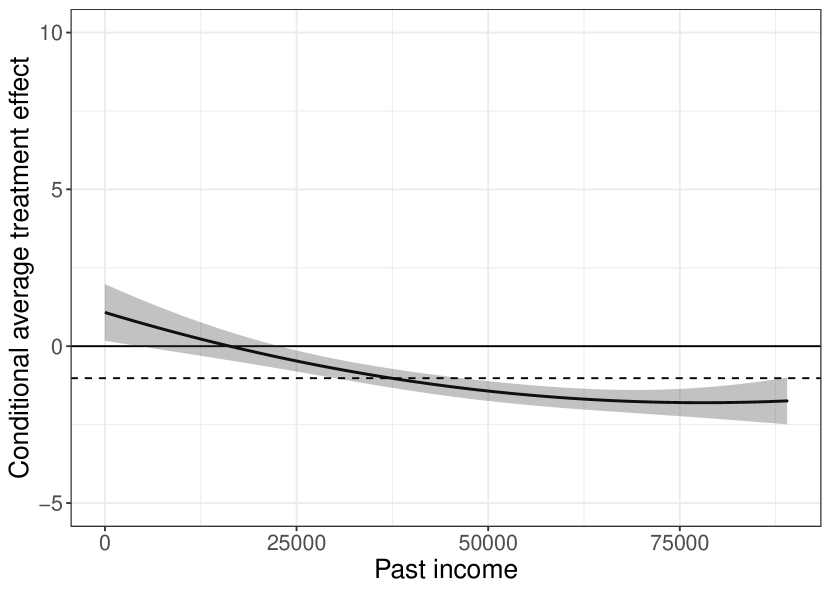
(b) Job search (Spline)

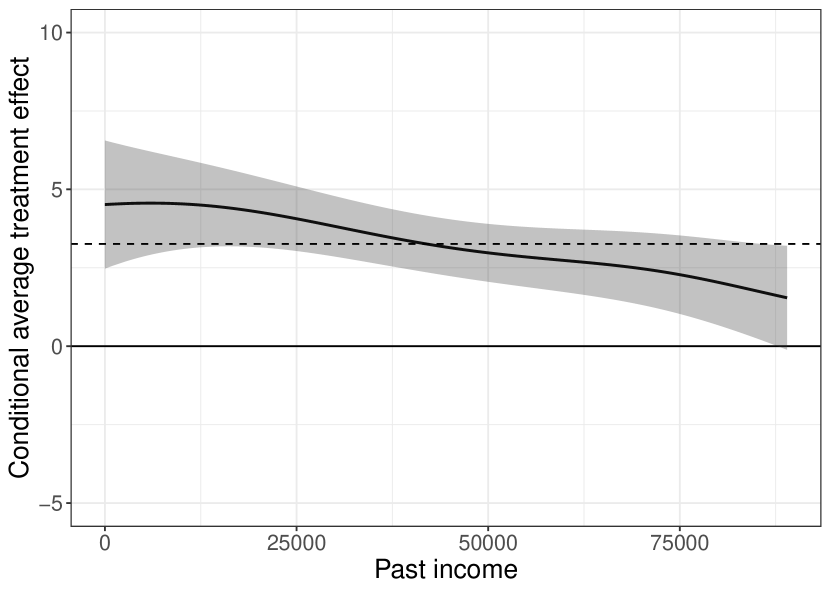
(c) Vocational (Kernel)

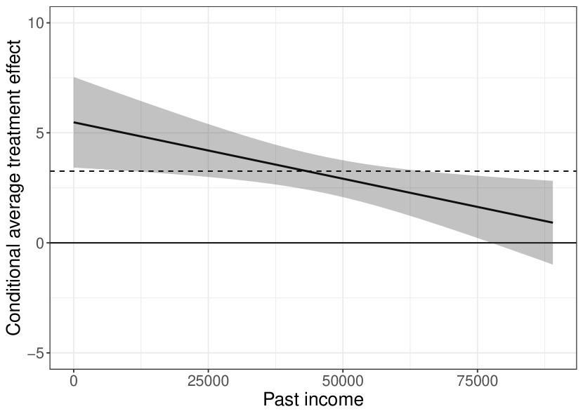
(d) Vocational (Spline)

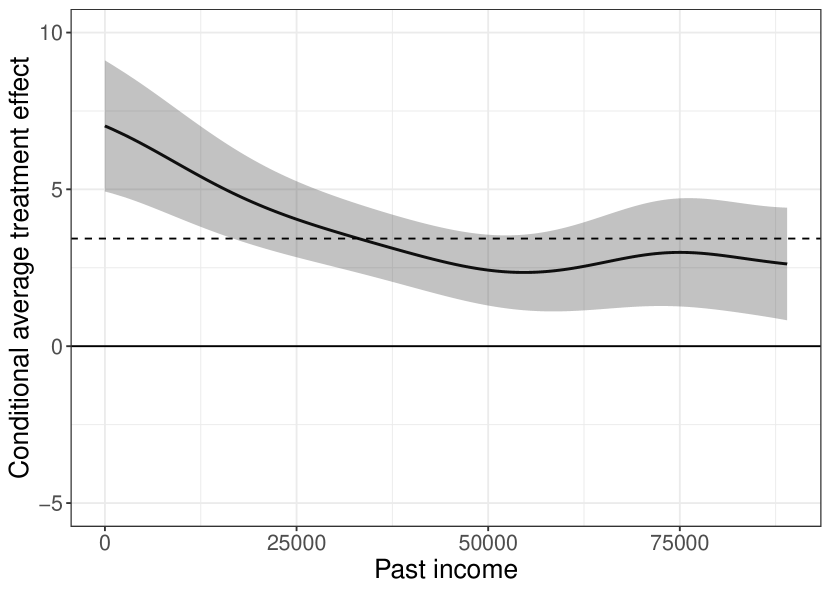
(e) Computer (Kernel)

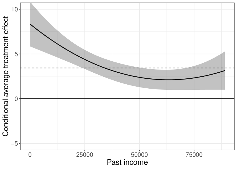
(f) Computer (Spline)

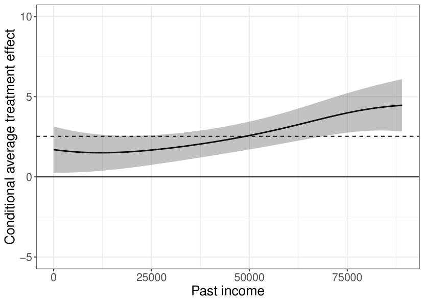
(g) Language (Kernel)

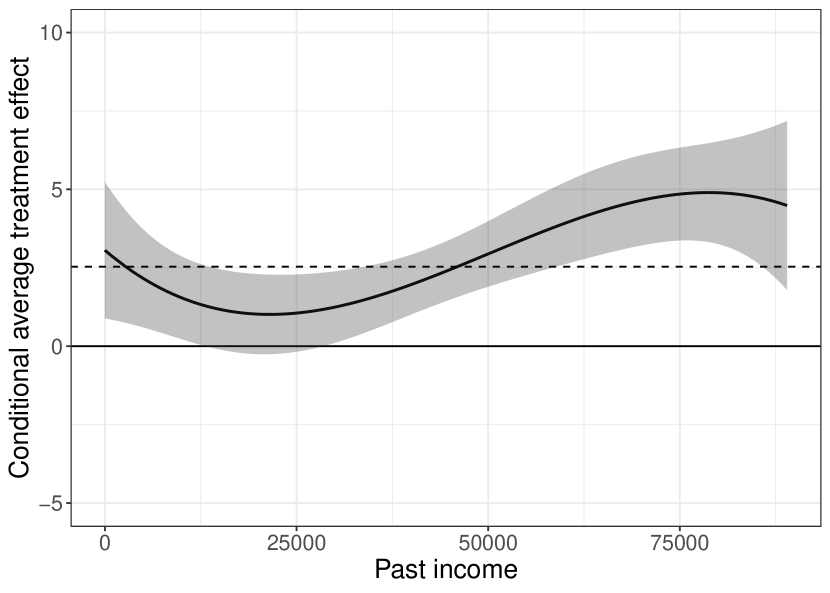
(h) Language (Spline)

(i) Note: Dotted line indicates point estimate of the respective average treatment effect. Grey area shows 95%-confidence interval.

While subgroup analyses are standard in program evaluations, the estimation of nonparametric GATEs using kernel or series regression is rarely pursued. We estimate such GATEs along two continuous variables past income and age. We find no notable heterogeneity for the latter. However, effect sizes are clearly associated with past income. Figure 3(i) shows on the left the results of the kernel regression and on the right of the series regression. Both estimators agree by and large. They document that effects decrease with higher past income for all but for language programs. The latter have only a small positive effect for individuals with low past income but it increases with higher income. One potential explanation for these findings is that the value of language skills is larger for high-skilled workers in multilingual countries like Switzerland because they reduce information costs across language borders <see, e.g.>Isphording2014LanguageSuccess.

Table 5: Best linear prediction of CATEs

	Job search	Vocational	Computer	Language
	(1)	(2)	(3)	(4)
Constant	-0.48	4.46∗	4.93∗∗	6.07∗∗∗
	(0.70)	(2.40)	(2.37)	(2.09)
Female	0.25	-2.12∗∗	1.89∗∗	-1.61∗∗
	(0.27)	(0.92)	(0.90)	(0.80)
Age	0.02	0.09∗	0.05	-0.07
	(0.01)	(0.05)	(0.05)	(0.05)
Foreigner	0.50∗	1.60∗	-1.20	-2.77∗∗∗
	(0.27)	(0.90)	(0.96)	(0.74)
Medium employability	-0.65∗	-1.64	-2.36∗	-0.78
	(0.37)	(1.18)	(1.22)	(0.99)
High employability	-1.03∗∗	-3.13∗∗	-3.15∗	-0.47
	(0.51)	(1.55)	(1.71)	(1.53)
Past income in CHF 10,000	-0.26∗∗∗	-0.62∗∗∗	-0.39∗∗	0.31∗
	(0.06)	(0.23)	(0.19)	(0.18)
F-statistic	6.95∗∗∗	4.12∗∗∗	3.35∗∗∗	5.22∗∗∗

• Note: This table shows OLS coefficients and their heteroscedasticity robust standard errors (in parentheses) of regressions run with the pseudo-outcome. ^∗p$<$0.1; ^∗∗p$<$0.05; ^∗∗∗p$<$0.01

6.2.3 Best linear prediction of GATEs

The GATEs considered so far were nonparametric but only univariate. Now we model the GATE by specifying a multivariate OLS regression with the previously used covariates entering linearly. It is most likely misspecified and thus estimates the best linear predictor (BLP) of GATEs with respect to these variables. However, it provides a compact and accessible summary of the effect heterogeneities. Additionally, it holds the other included variables constant. Consider for example the coefficients for being female in Table 5. Compared to Table 4, the coefficients in the first three columns are smaller and the one for language courses is larger (for example for job search it is 0.25 instead of 0.60). The reason is that it represents a partial effect that holds other variables like past income fixed. The subgroup female coefficient in Table 4 partly picks up that women have lower past income and that lower income is associated with higher treatment effects for all but language courses. This example illustrates that the same strategies that are usually applied to interpret an outcome OLS regression can now be used to interpret the effect OLS regression.

6.2.4 Individualised average treatment effects

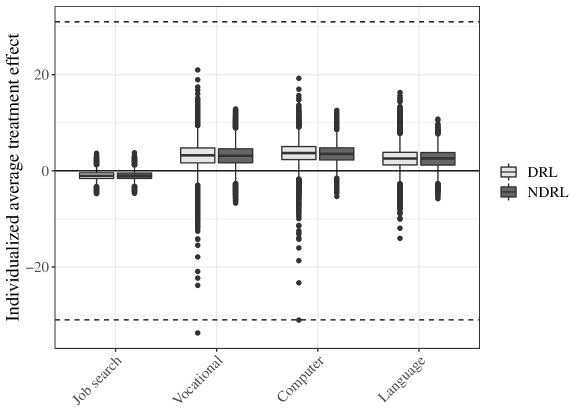
Figure 4: Boxplot of out-of-sample predicted IATEs by DR- and NDR-learner

(a) Note: The figure shows the distribution of IATEs for participating in the program labeled on the x-axis vs. non-participation estimated by the DR-learner (DRL) and the NDR-learner (NDRL). The dashed line indicates the possible range of the IATE of [-31,31] to illustrate that several DR-learner estimated IATEs lie outside this bound.

We focus on the results based on the out-of-sample variant of the DR- and NDR-learner as the full sample variant leads to severe overfitting with predicted IATEs ranging from -265 to 161 that are up to eight times larger than what is possible given that the outcome is bounded between zero and 31. However, Figure 4(a) shows that the DR-learner produces impossible effect sizes even out-of-sample, which motivates the proposal of the NDR-learner as stabilised variant. Figure 4(a) provides boxplots of the predicted IATEs and shows outliers lying below the smallest possible value of -31. However, the descriptive statistics provided in Table C.6 and the joint and marginal distributions depicted in Figure 6(e) document that besides the outliers the distributions are quite similar and correlate with at least 0.90. Not surprisingly, the impact of normalised weights is much larger for the three smaller programs and nearly negligible for job search programs. Still, we base the following discussion for all programs on the more stable results of the NDR-learner.

We conduct a classification analysis as proposed by Chernozhukov2018TheAverages to understand which variables are most predictive of effect sizes. To this end, we split the predicted IATE distributions in quintiles and compare the covariate means of the observations falling into the fifth and first quintile. For comparability, we normalise all covariates to have mean zero and variance one. Table 6 shows the seven variables that have at least one absolute difference between the highest and lowest quintile that is larger than one standard deviation. For example, we observe that the group with the highest effects (the fifth quintile) of a job search program has a 1.32 standard deviations lower past income compared to the lowest IATE group (the first quintile). Also the other variables confirm the patterns that we document already in previous subsections. The effects of job search, vocational and computer training are higher for unskilled workers with lower previous labour market success and foreigners, while the opposite holds for language programs.

Table 6: Classification analysis of IATEs

	Job search	Vocational	Computer	Language
	(1)	(2)	(3)	(4)
Past income	-1.32	-0.84	-1.17	1.01
Previous job: unskilled worker	1.02	0.68	0.34	-1.24
Mother tongue other than German, French, Italian	0.69	0.68	0.00	-1.17
Qualification: some degree	-0.88	-0.65	-0.41	1.15
Swiss citizen	-0.66	-0.60	0.12	1.11
Fraction of months employed last 2 years	-1.06	-0.37	-0.47	0.30
Qualification: unskilled	0.81	0.41	0.32	-1.02

• Note: Table shows the differences in means of standardized covariates between the fifth and the first quintile of the respective estimated IATE distribution.

6.3 Optimal treatment assignment

The previous section documented substantial heterogeneities in the program effects. To leverage this heterogeneity for better targeting, we apply the DML based optimal policy algorithm of Section 3.4. Figure 5(a) shows the simplest decision tree with only one split for the five handpicked covariates. It would allocate men to vocational training and women to computer courses. This split is probably similar to what we would have suggested given the evidence presented in Table 4. For a tree of depth two, such an eyeballing approach has its limits and the algorithmic approach provides a systematic way to arrive at an estimated optimal decision tree. The depth two tree in Figure 5(b) splits first on past income and then recommends to send low earning men to vocational and low earning women to computer training, while high earners (more than CHF 55k) are recommended to participate in language training. In the absence of the possibility to split on gender, the depth one tree in Figure 5(c) splits on past income roughly at the same value where the nonparametric GATEs of computer and language training intersect in Figure 3(i).

Figure 5: Optimal treatment assignment decision trees of depth two and three

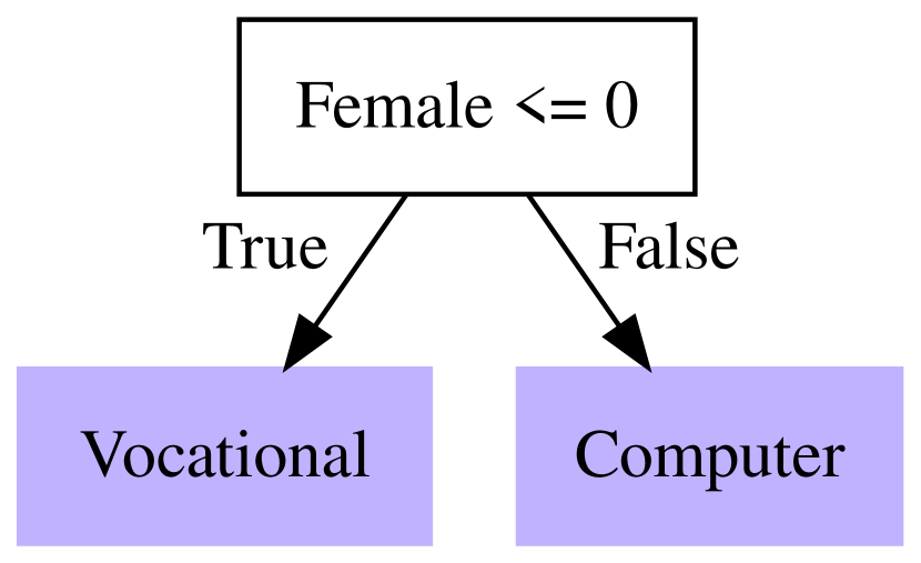
(a) Depth 1 & 5 covariates

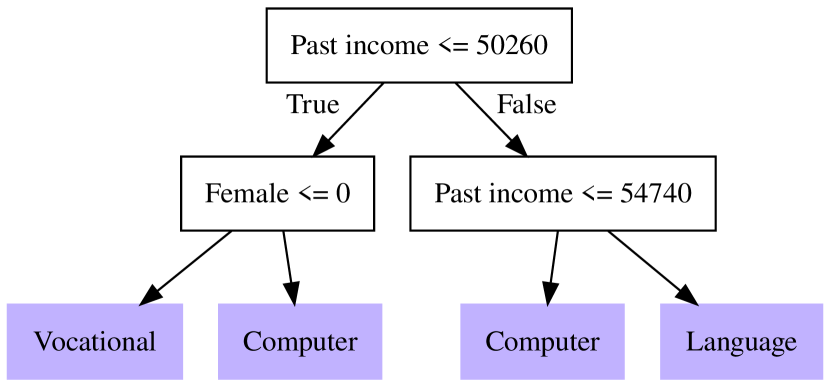
(b) Depth 2 & 5 covariates

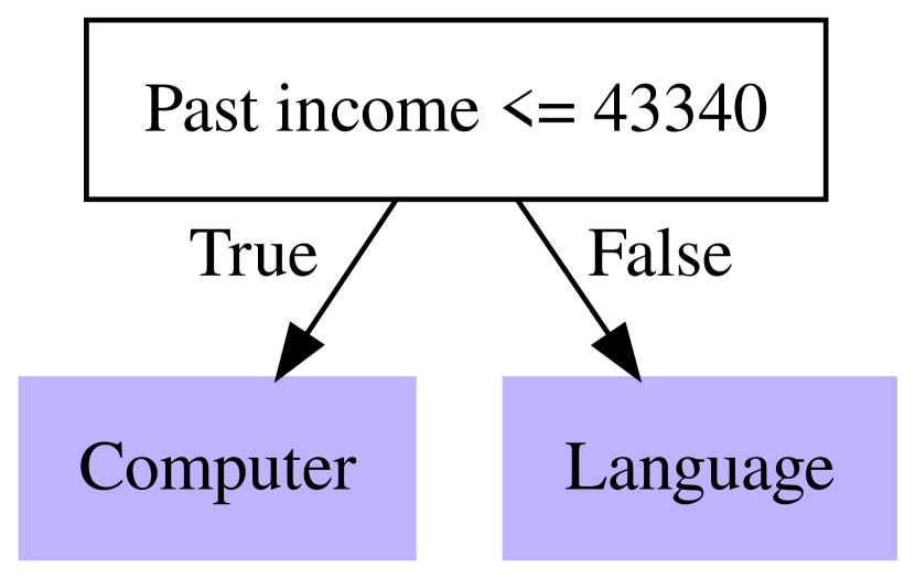
(c) Depth 1 & 16 covariates

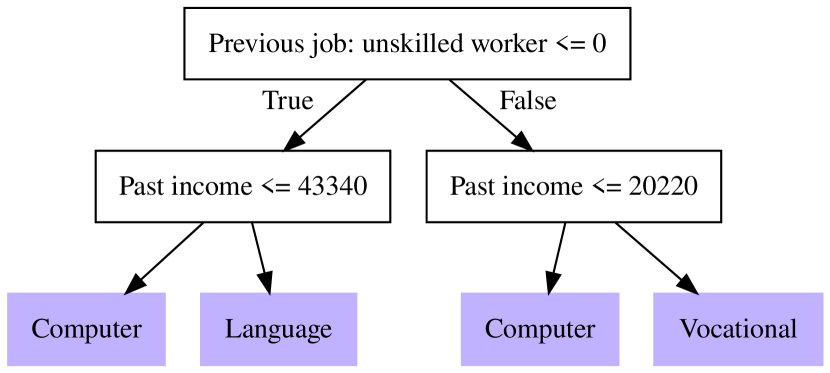
(d) Depth 2 & 16 covariates

(e) Notes: Optimal assignment rules estimated following the procedure defined in Section 3.4.

Panel A of Table 7 summarises the results of the different trees. It shows the percentage of individuals that are placed in the different programs. Not surprisingly, all individuals are recommended to be placed into one of the three positively evaluated hard skill enhancing programs.

One yet unsolved challenge is how to conduct statistical inference about the quality and stability of the decision trees. Athey2021PolicyData propose a form of cross-validation. To this end, we take the same folds that were used in the cross-fitting procedure to estimate the nuisance parameters. We build the decision tree in four folds and evaluate the value in the left out fold. First, we inspect how often the recommendations based on these trees coincide with the full sample policy rules. Figures C.8 and C.10 of Appendix C.6 show that the cross-validated trees are not identical to the full sample ones.

Table 7: Description of estimated optimal policies

	No program	Job search	Vocational	Computer	Language
	(1)	(2)	(3)	(4)	(5)
Panel A: Percent allocated to program
Depth 1 & 5 variables	0	0	56	44	0
Depth 2 & 5 variables	0	0	32	43	25
Depth 3 & 5 variables	0	0	47	37	17
Depth 1 & 16 variables	0	0	0	54	46
Depth 2 & 16 variables	0	0	23	37	40
Depth 3 & 16 variables	0	0	42	30	27
Panel B: Cross-validated difference to APOs
Depth 1 & 5 variables	3.75∗∗∗	4.77∗∗∗	0.49	0.32	1.21∗∗
	(0.40)	(0.42)	(0.44)	(0.48)	(0.49)
Depth 2 & 5 variables	3.99∗∗∗	5.01∗∗∗	0.73	0.56	1.45∗∗∗
	(0.40)	(0.42)	(0.48)	(0.46)	(0.46)
Depth 3 & 5 variables	3.50∗∗∗	4.52∗∗∗	0.24	0.07	0.96∗∗
	(0.41)	(0.43)	(0.45)	(0.49)	(0.47)
Depth 1 & 16 variables	3.72∗∗∗	4.73∗∗∗	0.46	0.29	1.19∗∗∗
	(0.41)	(0.42)	(0.52)	(0.48)	(0.40)
Depth 2 & 16 variables	3.63∗∗∗	4.65∗∗∗	0.37	0.20	1.10∗∗∗
	(0.43)	(0.44)	(0.47)	(0.53)	(0.42)
Depth 3 & 16 variables	3.94∗∗∗	4.96∗∗∗	0.68	0.51	1.41∗∗∗
	(0.42)	(0.43)	(0.47)	(0.49)	(0.46)

• Note: Panel A shows the percentage of individuals being assigned to a specific program. Panel B shows a t-test of the difference of the cross-validated policy (standard errors in parentheses) and the APOs of the programs. ^∗p$<$0.1; ^∗∗p$<$0.05; ^∗∗∗p$<$0.01

Zhou2018OfflineOptimization propose another validation idea and test whether the optimal policy rules perform significantly better than sending all individuals to the same program. This is achieved by taking the difference of the APO score of the cross-validated policy rule and the APO score of the program $w$: $\hat{\Delta}^{cv}_{i,w}(\pi)=\sum_{t=0}^{T}\mathds{1}(\hat{\pi}^{cv}(Z_{i})=t)\hat{\Gamma}_{i,t}-\hat{\Gamma}_{i,w}$, where $\hat{\pi}^{cv}(Z_{i})$ is the policy rule that is estimated without individual $i$. A standard t-test on the mean of $\hat{\Delta}^{cv}_{i,w}(\pi)$ tests then whether the cross-validated policy rules are significantly better than sending everybody to the same program. Note that the cross-validated policy rules do not necessarily coincide with the trees in the full sample and the cross-validation estimates not the value function for that specific tree. This requires to hold out a test set, which would be viable for an application with bigger programs.

The results are provided in Panel B of Table 7. We can interpret the mean of $\hat{\Delta}^{cv}_{i,w}(\pi)$ as average treatment effect comparing a regime under the estimated assignment rule or a regime where everybody is sent to the program $w$. This effect is always positive indicating that the estimated rules can leverage the effect heterogeneities to improve the allocation. However, the cross-validated policy rules perform not significantly better than sending just everybody into vocational or computer programs. This would probably change if we could take costs or capacity constraints into account. However, we do not observe costs in this dataset and the optimal decision tree algorithm is currently not capable of incorporating capacity constraints in a systematic way. We leave both extensions for future research using a more detailed database on both costs and capacity constraints.

7 Discussion and conclusions

This paper considers recent methodological developments based on Double Machine Learning (DML) through the lens of a standard program evaluation under unconfoundedness. DML based methods provide a convenient toolbox for a comprehensive program evaluation as different parameters of interest can be estimated using the same framework and a combination of standard statistical software. The application to an Active Labour Market Policy evaluation shows that the methods also produce plausible results in practice. The only exception is the DR-learner that required a modification, the newly introduced NDR-learner, before producing stable results for all individualised treatment effects. However, several conceptual and implementational issues remain open for investigation and refinement.

In general, we know little about how to choose the estimator for the nuisance parameters. The pool of potential machine learning algorithms and their combinations is large and little is known, e.g., about the trade-off between high prediction performance and computation time in the causal setting. Also clear recommendations for the implementation of cross-fitting are missing. Another open question is how to deal with common support in general and for each estimand specifically. The literature on trimming rules is well developed for propensity score based methods estimating average effects. However, we are not only interested in average effects and the propensity score is not the only nuisance parameter of DML. It remains an open question whether the established trimming methods are also sensible for DML when common support becomes an issue.

The estimators for flexible heterogeneous treatment effects provide interesting new tools. However, it is currently not clear to what extent we can actually explore heterogeneity or to what extent we need to pre-define the heterogeneity of interest. The possibility to summarise pre-defined heterogeneity of interest using OLS, kernel or series regressions provide clearly valuable and easy to use options in applications. The instability of methods that aim for individualised heterogeneous effects shows that they should be used with caution and more research is required to investigate whether adjustments like the proposed NDR-learner are useful beyond the application of this paper.

The estimation of optimal treatment assignment rules is mostly unexplored in practice and many interesting issues in applications regarding inference, the implementation of different constraints, more flexible rules than decision trees, or the choice of variables that could or should enter the set of policy variables, which could be explored in future research.

The investigation of these DML specific questions but also the comparison with other more specialised causal machine learning methods for each estimand provides another interesting direction of future research. Such evidence would help to understand and guide which choices are critical in applications similar to the one in this paper.

Appendices

Appendix A Identification and Neyman orthogonality

A.1 Doubly robust identification

To revisit identification and identification double robustness of Equation 2.3 under Assumption 2.1, rewrite the conditional average potential outcome in the following way, where $\mu_{w}(x)=E[Y_{i}(w)\mid X_{i}=x]$, $\mu(w,x)=E[Y_{i}\mid W_{i}=w,X_{i}=x]$ and $e_{w}(x)=E\left[D_{i}(w)\middle|X_{i}=x\right]=P\left[W_{i}=w\middle|X_{i}=x\right]\overset{1b}{>}0$:

$$\mu_{w}(x) =E\left[\mu(w,x)+\dfrac{D_{i}(w)(Y_{i}-\mu(w,x))}{e_{w}(x)}\middle|X_{i}=x\right]$$

$$=E\left[Y_{i}(w)-Y_{i}(w)+\mu(w,x)+\dfrac{D_{i}(w)(Y_{i}-\mu(w,x))}{e_{w}(x)}\middle|X_{i}=x\right]$$

$$\overset{\mathrm{1c}}{=}E\left[Y_{i}(w)-Y_{i}(w)+\mu(w,x)+\dfrac{D_{i}(w)(Y_{i}(w)-\mu(w,x))}{e_{w}(x)}\middle|X_{i}=x\right]$$

$$=E\left[Y_{i}(w)\mid X_{i}=x\right]+E\left[\left(Y_{i}(w)-\mu(w,x)\right)\left(\dfrac{D_{i}(w)-e_{w}(x)}{e_{w}(x)}\right)\middle|X_{i}=x\right]$$

$$=\mu_{w}(x)+E\left[\left(Y_{i}(w)-\mu(w,x)\right)\left(\dfrac{D_{i}(w)-e_{w}(x)}{e_{w}(x)}\right)\middle|X_{i}=x\right]$$ (10)

The conditional average potential outcome is thus identified if the second part of Equation 10 equals zero. This happens under three scenarios:

1. Correct propensity score and correct outcome regression:

$$E \left[\left(Y_{i}(w)-\mu(w,x)\right)\left(\dfrac{D_{i}(w)-e_{w}(x)}{e_{w}(x)}\right)\middle|X_{i}=x\right]$$

$$\overset{\mathrm{1a}}{=}E\left[\left(Y_{i}(w)-\mu(w,x)\right)\middle|X_{i}=x\right]E\left[\left(\dfrac{D_{i}(w)-e_{w}(x)}{e_{w}(x)}\right)\middle|X_{i}=x\right]$$

$$=\left(E\left[Y_{i}(w)\mid X_{i}=x\right]-\mu(w,x)\right)\left(\dfrac{E\left[D_{i}(w)\mid X_{i}=x\right]-e_{w}(x)}{e_{w}(x)}\right)$$

$$=\left(\mu_{w}(x)-\mu(w,x)\right)\left(\dfrac{e_{w}(x)-e_{w}(x)}{e_{w}(x)}\right)$$

$$\overset{\mathrm{1a}}{=}\underbrace{\left(\mu_{w}(x)-\mu_{w}(x)\right)}_{=0}\underbrace{\left(\dfrac{e_{w}(x)-e_{w}(x)}{e_{w}(x)}\right)}_{=0}=0$$

2. Correct propensity score but instead of correct outcome regression $\mu(w,x)$, use some function $g(x)$:

$$E \left[\left(Y_{i}(w)-g(x)\right)\left(\dfrac{D_{i}(w)-e_{w}(x)}{e_{w}(x)}\right)\middle|X_{i}=x\right]$$

$$\overset{\mathrm{1a}}{=}E\left[\left(Y_{i}(w)-g(x)\right)\middle|X_{i}=x\right]E\left[\left(\dfrac{D_{i}(w)-e_{w}(x)}{e_{w}(x)}\right)\middle|X_{i}=x\right]$$

$$=\left(E\left[Y_{i}(w)\mid X_{i}=x\right]-g(x)\right)\left(\dfrac{E\left[D_{i}(w)\mid X_{i}=x\right]-e_{w}(x)}{e_{w}(x)}\right)$$

$$=\left(\mu_{w}(x)-g(x)\right)\underbrace{\left(\dfrac{e_{w}(x)-e_{w}(x)}{e_{w}(x)}\right)}_{=0}=0$$

3. Correct outcome regression but instead of correct propensity score $e_{w}(x)$, use some function $h(x)$:

$$E \left[\left(Y_{i}(w)-\mu(w,x)\right)\left(\dfrac{D_{i}(w)-h(x)}{h(x)}\right)\middle|X_{i}=x\right]$$

$$\overset{\mathrm{1a}}{=}E\left[\left(Y_{i}(w)-\mu(w,x)\right)\middle|X_{i}=x\right]E\left[\left(\dfrac{D_{i}(w)-h(x)}{h(x)}\right)\middle|X_{i}=x\right]$$

$$=\left(E\left[Y_{i}(w)\mid X_{i}=x\right]-\mu(w,x)\right)\left(\dfrac{E\left[D_{i}(w)\mid X_{i}=x\right]-h(x)}{h(x))}\right)$$

$$=\left(\mu_{w}(x)-\mu(w,x)\right)\left(\dfrac{e_{w}(x)-h(x)}{h(x)}\right)$$

$$\overset{\mathrm{1a}}{=}\underbrace{\left(\mu_{w}(x)-\mu_{w}(x)\right)}_{=0}\left(\dfrac{e_{w}(x)-h(x)}{h(x)}\right)=0$$

A.2 Neyman orthogonality

We revisit Neyman orthogonality of the APO score as the other scores follow similarly. The score defining the APO is

$$E\Bigg{[}\underbrace{\mu(w,X_{i})+\frac{D_{i}(w)(Y_{i}-\mu(w,X_{i}))}{e_{w}(X_{i})}-\gamma_{w}}_{\psi(Y_{i},W_{i},\mu(w,X_{i}),e_{w}(X_{i}))}\Bigg{]}=0$$ (11)

$$\Rightarrow\leavevmode\nobreak\ \leavevmode\nobreak\ \gamma_{w}=E\Bigg{[}\mu(w,X_{i})+\frac{D_{i}(w)(Y_{i}-\mu(w,X_{i}))}{e_{w}(X_{i})}\Bigg{]}$$ (12)

Neyman-orthogonality of a score $\psi(\cdot)$ means that the Gateaux derivative with respect to the nuisance parameters is zero in expectation at the true nuisance parameters (NP). In our case this means that

$$\partial_{r}E[\psi(Y_{i},W_{i},\mu+r(\tilde{\mu}-\mu),e+r(\tilde{e}-e))|X_{i}=x]|_{r=0}=0$$ (13)

where we suppress the dependencies of NPs and denote by, e.g., $\tilde{\mu}$ a value of the outcome nuisance that is different to the true value $\mu$. We can show that Equation 13 holds with the following steps:

First, add perturbations to the true nuisance parameters in the score

$$\psi (Y_{i},W_{i},\mu+r(\tilde{\mu}-\mu),e+r(\tilde{e}-e))$$

$$=(\mu+r(\tilde{\mu}-\mu))+\frac{D_{i}(w)Y_{i}}{e+r(\tilde{e}-e)}-\frac{D_{i}(w)(\mu+r(\tilde{\mu}-\mu))}{e+r(\tilde{e}-e)}-\gamma_{w}$$

Second, take the conditional expectation

$$E \left[\psi(Y_{i},W_{i},\mu+r(\tilde{\mu}-\mu),e+r(\tilde{e}-e))\middle|X_{i}=x\right]$$

$$=E\left[(\mu+r(\tilde{\mu}-\mu))+\frac{D_{i}(w)Y_{i}}{e+r(\tilde{e}-e)}-\frac{D_{i}(w)(\mu+r(\tilde{\mu}-\mu))}{e+r(\tilde{e}-e)}-\hat{\gamma}_{w}\middle|X_{i}=x\right]$$

$$=(\mu+r(\tilde{\mu}-\mu))+\frac{e\mu}{e+r(\tilde{e}-e)}-\frac{e(\mu+r(\tilde{\mu}-\mu))}{e+r(\tilde{e}-e)}-\gamma_{w}$$

where we use that $E[D_{i}(w)Y_{i}\mid X_{i}=x]=E[D_{i}(w)\sum_{w}D_{i}(w)Y_{i}(w)\mid X_{i}=x]=E[D_{i}(w)Y_{i}(w)\mid X_{i}=x]\overset{1a}{=}e\mu$.

Third, take the derivative with respect to $r$

$$\partial_{r}E \left[\psi(Y_{i},W_{i},\mu+r(\tilde{\mu}-\mu),e+r(\tilde{e}-e))\middle|X_{i}=x\right]$$

$$=(\tilde{\mu}-\mu)-\frac{e\mu(\tilde{e}-e)}{(e+r(\tilde{e}-e))^{2}}-\frac{e(\tilde{\mu}-\mu)(e+r(\tilde{e}-e))-e(\mu+r(\tilde{\mu}-\mu))(\tilde{e}-e)}{(e+r(\tilde{e}-e))^{2}}$$

Finally, evaluate at the true nuisance values, i.e. set $r=0$ to show that 13 holds

$$\partial_{r} E[\psi(Y_{i},W_{i},\mu+r(\tilde{\mu}-\mu),e+r(\tilde{e}-e))|X_{i}=x]|_{r=0}$$

$$=(\tilde{\mu}-\mu)-\frac{e\mu(\tilde{e}-e)}{(e+0(\tilde{e}-e))^{2}}-\frac{e(\tilde{\mu}-\mu)(e+0(\tilde{e}-e))-e(\mu+0(\tilde{\mu}-\mu))(\tilde{e}-e)}{(e+0(\tilde{e}-e))^{2}}$$

$$=(\tilde{\mu}-\mu)-\frac{e\mu(\tilde{e}-e)}{e^{2}}-\frac{e(\tilde{\mu}-\mu)e-e\mu(\tilde{e}-e)}{e^{2}}$$

$$=(\tilde{\mu}-\mu)-\frac{e\mu(\tilde{e}-e)}{e^{2}}-\frac{e^{2}}{e^{2}}(\tilde{\mu}-\mu)+\frac{e\mu(\tilde{e}-e)}{e^{2}}$$

$$=0$$

Appendix B DR- and NDR-learner

This Appendix describes the algorithms that are applied to estimate out-of-sample IATEs using the DR- and NDR-learner. It mostly follows Algorithm 1 of Kennedy2020OptimalEffects and adapts it to the situation that we are interested in estimating IATEs for all observations without using them in the estimation step.

Algorithm 1 (DR-learner)

Let $(S_{1}^{N},S_{2}^{N},S_{3}^{N},S_{4}^{N})$ denote four independent samples of $N$ observations of $O_{i}=(X_{i},W_{i},Y_{i})$.

1. Nuisance training:

   1. Construct a model $\hat{e}_{w}(x)$ of the propensity scores $e_{w}(x)$ using $S_{1}^{N}$.

   2. Construct a model $(\hat{\mu}(w,x),\hat{\mu}(w^{\prime},x))$ of the regression functions $(\mu(w,x),\mu(w^{\prime},x))$ using $S_{2}^{N}$.

2. Pseudo-outcome regression: Construct the pseudo-outcome for every observation $i$ in subsample $S_{3}^{N}$ using the models of step 1

   $$\hat{\Delta}_{i,w,w^{\prime}}=\hat{\mu}(w,X_{i})-\hat{\mu}(w^{\prime},X_{i})+\dfrac{D_{i}(w)}{\hat{e}_{w}(X_{i})}\tilde{Y_{i}}(w,X_{i})-\dfrac{D_{i}(w^{\prime})}{\hat{e}_{w^{\prime}}(X_{i})}\tilde{Y_{i}}(w^{\prime},X_{i}),$$

   regress it on covariates $X_{i}$ in $S_{3}^{N}$, and use the model to predict IATEs in $S_{4}^{N}$, $\hat{\tau}_{w,w^{\prime}}^{4,1}(x)$.

3. Cross-fitting: Repeat steps 1–2 twice, first using $S_{2}^{N}$ for the propensity score, $S_{3}^{N}$ for the outcome regression and $S_{1}^{N}$ as subsample to obtain IATE predictions in $S_{4}^{N}$ $\hat{\tau}_{w,w^{\prime}}^{4,2}(x)$, and then using $S_{3}^{N}$ for the propensity score, $S_{1}^{N}$ for the outcome regression and $S_{2}^{N}$ as subsample to obtain IATE predictions in $S_{4}^{N}$, $\hat{\tau}_{w,w^{\prime}}^{4,3}(x)$.

4. Prediction: Predict IATEs in $S_{4}^{N}$ as the average of the three predictions $\hat{\tau}_{w,w^{\prime}}^{drl}(x)=1/3\hat{\tau}_{w,w^{\prime}}^{4,1}(x)+1/3\hat{\tau}_{w,w^{\prime}}^{4,2}(x)+1/3\hat{\tau}_{w,w^{\prime}}^{4,3}(x)$.

5. Iteration: Repeat steps 1–4 three times. First, with $S_{1}^{N}$, $S_{2}^{N}$ and $S_{4}^{N}$ to predict IATEs for $S_{3}^{N}$, second with $S_{1}^{N}$, $S_{3}^{N}$ and $S_{4}^{N}$ to predict IATEs for $S_{2}^{N}$ and finally with $S_{2}^{N}$, $S_{3}^{N}$ and $S_{4}^{N}$ to predict IATEs for $S_{1}^{N}$.

The NDR-learner follows the same basic steps but modifies step two:

Algorithm 2 (NDR-learner)

Let $(S_{1}^{N},S_{2}^{N},S_{3}^{N},S_{4}^{N})$ denote four independent samples of $N$ observations of $O_{i}=(X_{i},W_{i},Y_{i})$.

1. Nuisance training:

   1. Construct a model $\hat{e}_{w}(x)$ of the propensity scores $e_{w}(x)$ using $S_{1}^{N}$.

   2. Construct a model $(\hat{\mu}(w,x),\hat{\mu}(w^{\prime},x))$ of the regression functions $(\mu(w,x),\mu(w^{\prime},x))$ using $S_{2}^{N}$.

2. Pseudo-outcome regression: Construct the pseudo-outcome for every observation $i$ in subsample $S_{3}^{N}$ using the models of step 1

   $$\hat{\Delta}_{i,w,w^{\prime}}=\hat{\mu}(w,X_{i})-\hat{\mu}(w^{\prime},X_{i})+\dfrac{D_{i}(w)}{\hat{e}_{w}(X_{i})}\tilde{Y_{i}}(w,X_{i})-\dfrac{D_{i}(w^{\prime})}{\hat{e}_{w^{\prime}}(X_{i})}\tilde{Y_{i}}(w^{\prime},X_{i}),$$

   regress it on covariates $X_{i}$ in $S_{3}^{N}$, and use the model to predict IATEs in $S_{4}^{N}$.

3. Normalisation: For every observation $j$ in $S_{4}^{N}$: (i) extract the weights underlying its prediction $\alpha_{i}(X_{j})$ and (ii) use it to calculate the normalised DR-learner given in Equation 3.9, where the sum goes over observations in $S_{3}^{N}$, to obtain $\hat{\tau}_{w,w^{\prime}}^{4,1}(X_{j})$.

4. Cross-fitting: Repeat steps 1–2 twice, first using $S_{2}^{N}$ for the propensity score, $S_{3}^{N}$ for the outcome regression and $S_{1}^{N}$ as subsample to obtain IATE predictions in $S_{4}^{N}$ $\hat{\tau}_{w,w^{\prime}}^{4,2}(x)$, and then using $S_{3}^{N}$ for the propensity score, $S_{1}^{N}$ for the outcome regression and $S_{2}^{N}$ as subsample to obtain IATE predictions in $S_{4}^{N}$, $\hat{\tau}_{w,w^{\prime}}^{4,3}(x)$.

5. Prediction: Predict IATEs in $S_{4}^{N}$ as the average of the three predictions $\hat{\tau}_{w,w^{\prime}}^{drl}(x)=1/3\hat{\tau}_{w,w^{\prime}}^{4,1}(x)+1/3\hat{\tau}_{w,w^{\prime}}^{4,2}(x)+1/3\hat{\tau}_{w,w^{\prime}}^{4,3}(x)$.

6. Iteration: Repeat steps 1–4 three times. First, with $S_{1}^{N}$, $S_{2}^{N}$ and $S_{4}^{N}$ to predict IATEs for $S_{3}^{N}$, second with $S_{1}^{N}$, $S_{3}^{N}$ and $S_{4}^{N}$ to predict IATEs for $S_{2}^{N}$ and finally with $S_{2}^{N}$, $S_{3}^{N}$ and $S_{4}^{N}$ to predict IATEs for $S_{1}^{N}$.

Appendix C Results

C.1 Descriptives

Table C.1 provides the means of all confounders by program participation. It documents that especially measures of past labour market success like past income are associated with program participation.

[t]

Table C.1: Means of control variables by program

	No	JS	Voc	Comp	Lang
	(1)	(2)	(3)	(4)	(5)
Age	36.6	37.3	37.5	39.1	35.3
Mother tongue in canton’s language	0.10	0.12	0.11	0.11	0.04
Lives in big city	0.19	0.19	0.21	0.11	0.23
Lives in medium city	0.12	0.13	0.12	0.15	0.15
Lives in no city	0.68	0.68	0.67	0.73	0.63
Caseworker age	44.1	44.1	44.8	44.6	44.6
Caseworker cooperative	0.48	0.50	0.41	0.42	0.45
Caseworker education: above vocational training	0.46	0.45	0.44	0.48	0.48
Caseworker education: tertiary track	0.19	0.21	0.17	0.16	0.21
Caseworker female	0.43	0.47	0.39	0.44	0.47
Missing caseworker characteristics	0.05	0.05	0.04	0.05	0.05
Caseworker has own unemployemnt experience	0.62	0.63	0.64	0.61	0.63
Caseworker tenure	5.48	5.44	5.73	5.83	5.61
Caseworker education: vocational degree	0.26	0.27	0.22	0.25	0.22
Fraction of months employed last 2 years	0.81	0.84	0.83	0.84	0.72
Number of employment spells last 5 years	1.21	0.97	0.93	0.86	0.78
Employability	1.93	1.98	1.93	1.97	1.85
Female	0.44	0.44	0.33	0.60	0.55
Foreigner with temporary permit	0.13	0.11	0.12	0.04	0.44
Foreigner with permanent permit	0.23	0.22	0.18	0.17	0.23
Cantonal GDP p.c.	0.52	0.53	0.51	0.53	0.54
Married	0.47	0.46	0.48	0.45	0.72
Mother tongue other than German, French, Italian	0.33	0.29	0.31	0.18	0.64
Past income	42528.0	46693.1	48653.8	43212.8	37300.5
Previous job: manager	0.08	0.08	0.10	0.09	0.07
Missing sector	0.18	0.15	0.15	0.16	0.29
Previous job in primary sector	0.09	0.06	0.09	0.05	0.05
Previous job in secondary sector	0.12	0.14	0.15	0.13	0.12
Previous job in tertiary sector	0.61	0.65	0.61	0.67	0.54
Previous job: self-employed	0.01	0.00	0.00	0.00	0.00
Previous job: skilled worker	0.60	0.65	0.65	0.75	0.43
Previous job: unskilled worker	0.29	0.24	0.22	0.15	0.48
Qualification: semiskilled	0.16	0.14	0.17	0.14	0.15
Qualification: some degree	0.58	0.62	0.63	0.72	0.38
Qualification: unskilled	0.23	0.20	0.17	0.12	0.40
Qualification: skilled without degree	0.03	0.03	0.02	0.02	0.07
Swiss citizen	0.64	0.67	0.70	0.79	0.34
Allocation of unemployed to caseworkers: by industry	0.60	0.67	0.58	0.51	0.64
Allocation of unemployed to caseworkers: by occupation	0.51	0.57	0.46	0.45	0.57
Allocation of unemployed to caseworkers: by age	0.04	0.04	0.04	0.06	0.05
Allocation of unemployed to caseworkers: by employability	0.09	0.07	0.10	0.08	0.06
Allocation of unemployed to caseworkers: by region	0.13	0.09	0.09	0.13	0.11
Allocation of unemployed to caseworkers: other	0.09	0.07	0.08	0.10	0.09
Number of unemployment spells last 2 years	0.57	0.39	0.52	0.37	0.43
Cantonal unemployment rate (in %)	3.52	3.59	3.41	3.36	3.63

• Note: Program specific means.

C.2 Nuisance parameters

Nuisance parameters are only a tool to remove confounding but it is still informative to investigate which variables are most predictive of treatment probabilities and outcome. This is less straightforward for flexible tools like random forests than for the well-known regression outputs of parametric models. We conduct a classification analysis as proposed by Chernozhukov2018TheAverages. To this end, we split the predicted nuisance parameter distributions in quintiles and compare the covariate means of the observations falling into the fifth and first quintile. For comparability, we normalise all covariates to have mean zero and variance one and order the variables by their largest absolute difference between the highest and lowest quintile.

Table C.2 shows that measures of citizenship, qualification and previous labour market success are important predictors of program selection. In line with intuition the former seems to drive a large part of the selection into language courses. Also Table C.3 showing the classification analysis for outcome predictions shows intuitive patterns. Again measures of citizenship, qualification and previous labour market success seem predictive for future employment with suggested correlations pointing in the expected directions. For example, Swiss citizens, individuals with a degree and high past income are overrepresented in the upper quintile, while individuals with a non-Swiss mother tongue and no qualification are underepresented in the upper quintile.

Finally, we investigate the propensity score distributions for all programs. Figure C.1 shows that propensity scores are quite variable. This indicates that selection into programs is not negligible. Further, Table C.4 shows that some of the propensity scores get quite small with the smallest one being 0.003 for a computer training participant. This is not surprising given that already the unconditional participation probabilities for computer and vocational training are only about 0.015. However, the small propensity score per se is not an indicator of poor overlap. The residual with the smallest propensity score receives a weight of $\sim 1/0.003=333$, which is only 0.5% of the total weights. Note that we could easily increase the smallest propensity score by randomly removing a large fraction of non-participants and participants of the job search program. This would discard valuable information and shows that the mere focus on the smallest propensity score can be misleading in cases with imbalanced treatment group sizes. More importantly, we observe overlap in the sense that all treatment groups contain individuals with similarly low propensity scores. Thus, overlap seems not to be a major issue in our application, at least for the low dimensional parameters of interest.

[t]

Table C.2: Classification analysis of propensity scores

	No program	Job search	Vocational	Computer	Language
	(1)	(2)	(3)	(4)	(5)
Foreigner with temporary permit	-0.22	-0.34	-0.32	-1.25	1.93
Swiss citizen	0.08	0.22	0.43	1.59	-1.86
Mother tongue other than German, French, Italian	0.10	-0.42	-0.33	-1.57	1.76
Previous job: unskilled worker	0.31	-0.43	-0.61	-1.52	0.99
Past income	-0.72	0.78	1.42	0.28	-0.07
Previous job: skilled worker	-0.20	0.31	0.30	1.31	-0.90
Qualification: some degree	-0.18	0.31	0.53	1.26	-0.93
Qualification: unskilled	0.04	-0.16	-0.55	-1.16	0.86
Female	-0.08	-0.06	-1.07	1.00	0.41
Married	-0.23	-0.03	-0.17	-0.60	1.07
Cantonal unemployment rate (in %)	-0.71	0.73	-0.90	-0.53	-0.14
Foreigner with permanent permit	0.08	0.03	-0.23	-0.81	0.56
Age	-0.34	0.33	0.35	0.79	-0.25
Cantonal GDP p.c.	-0.62	0.65	-0.73	-0.16	-0.14
Number of employment spells last 5 years	0.73	-0.53	-0.41	-0.46	-0.31
Allocation of unemployed to caseworkers: by occupation	-0.49	0.50	-0.64	-0.21	0.08
Allocation of unemployed to caseworkers: by region	0.53	-0.53	0.02	0.06	0.03
Fraction of months employed last 2 years	-0.26	0.47	0.53	0.40	-0.45
Allocation of unemployed to caseworkers: by industry	-0.45	0.45	-0.49	-0.53	0.01
Previous job: manager	-0.21	0.18	0.52	0.17	0.09
Employability	-0.44	0.49	0.14	0.36	-0.25
Previous job in tertiary sector	-0.20	0.27	0.01	0.45	-0.31
Caseworker cooperative	-0.08	0.11	-0.43	-0.21	-0.02
Missing sector	0.15	-0.29	-0.41	-0.35	0.43
Lives in big city	0.07	-0.08	-0.04	-0.42	0.09
Number of unemployment spells last 2 years	0.39	-0.33	-0.06	-0.40	0.02
Caseworker female	-0.30	0.27	-0.39	0.14	-0.03
Qualification: skilled without degree	-0.08	-0.02	-0.10	-0.27	0.36
Lives in no city	-0.01	0.05	-0.02	0.33	-0.12
Previous job in primary sector	0.30	-0.26	0.30	-0.26	-0.02
Caseworker tenure	-0.02	0.00	0.24	0.12	0.05
Qualification: semiskilled	0.24	-0.22	-0.04	-0.24	0.10
Previous job in secondary sector	-0.13	0.15	0.21	-0.05	-0.02
Caseworker age	-0.05	0.03	0.12	0.08	0.19
Allocation of unemployed to caseworkers: by employability	0.18	-0.19	0.11	0.01	-0.01
Caseworker education: tertiary track	-0.18	0.18	-0.12	-0.17	0.00
Caseworker has own unemployemnt experience	-0.14	0.16	0.07	-0.02	0.02
Caseworker education: vocational degree	-0.10	0.14	-0.15	0.07	-0.14
Mother tongue in canton’s language	-0.01	0.10	-0.03	0.03	0.14
Allocation of unemployed to caseworkers: other	0.05	-0.04	-0.13	-0.00	-0.07
Caseworker education: above vocational training	0.12	-0.13	0.04	0.11	0.02
Allocation of unemployed to caseworkers: by age	-0.02	0.01	-0.06	0.08	-0.00
Lives in medium city	-0.07	0.02	0.06	0.03	0.06
Previous job: self-employed	0.01	0.01	0.02	0.04	-0.07
Missing caseworker characteristics	0.06	-0.06	0.05	-0.02	0.00

• Note: Table shows the differences in means of normalized covariates between the fifth and the first quintile of the respective propensity score distribution. Variables are ordered according to the largest absolute difference.

[t]

Table C.3: Classification analysis of outcome predictions

	No program	Job search	Vocational	Computer	Language
	(1)	(2)	(3)	(4)	(5)
Mother tongue other than German, French, Italian	-1.44	-1.66	-1.16	-2.06	-1.89
Qualification: some degree	1.80	1.96	1.57	1.64	1.85
Swiss citizen	1.37	1.60	1.13	1.94	1.83
Previous job: unskilled worker	-1.72	-1.76	-1.55	-1.65	-1.87
Past income	1.49	1.38	1.16	0.87	1.73
Qualification: unskilled	-1.43	-1.57	-1.53	-1.36	-1.52
Previous job: skilled worker	1.23	1.27	1.21	1.34	1.36
Foreigner with permanent permit	-0.88	-1.11	-0.71	-1.34	-1.15
Number of unemployment spells last 2 years	-0.93	-0.80	-1.25	-0.57	-0.56
Married	-0.98	-1.14	-0.60	-1.19	-1.04
Foreigner with temporary permit	-0.84	-0.89	-0.72	-1.08	-1.16
Fraction of months employed last 2 years	1.01	0.78	0.91	0.66	0.87
Employability	0.93	0.84	0.46	0.49	0.62
Age	-0.72	-0.76	-0.25	-0.34	-0.29
Cantonal unemployment rate (in %)	-0.10	-0.05	-0.75	-0.02	-0.04
Lives in big city	-0.24	-0.22	-0.74	-0.36	-0.30
Cantonal GDP p.c.	-0.04	0.02	-0.74	0.04	0.06
Missing sector	-0.50	-0.48	-0.58	-0.53	-0.71
Number of employment spells last 5 years	-0.54	-0.42	-0.68	-0.45	-0.41
Lives in no city	0.26	0.23	0.68	0.43	0.33
Previous job: manager	0.54	0.52	0.40	0.32	0.67
Qualification: semiskilled	-0.63	-0.67	-0.26	-0.49	-0.59
Female	-0.42	-0.32	-0.44	0.23	-0.60
Previous job in tertiary sector	0.31	0.36	0.14	0.50	0.51
Mother tongue in canton’s language	-0.21	-0.25	-0.22	-0.45	-0.33
Allocation of unemployed to caseworkers: by occupation	0.18	0.22	0.32	0.39	0.25
Qualification: skilled without degree	-0.35	-0.38	-0.22	-0.34	-0.35
Previous job in secondary sector	0.08	0.05	0.31	0.01	0.07
Caseworker age	0.02	0.03	0.27	-0.17	0.07
Caseworker female	0.01	0.04	-0.20	0.26	-0.02
Caseworker tenure	-0.05	-0.06	-0.11	-0.25	-0.06
Previous job in primary sector	0.05	-0.04	0.18	-0.17	-0.01
Lives in medium city	-0.08	-0.05	-0.08	-0.17	-0.12
Caseworker education: vocational degree	0.11	0.08	0.15	0.07	0.08
Allocation of unemployed to caseworkers: by employability	0.04	0.03	0.15	0.05	0.04
Allocation of unemployed to caseworkers: by industry	0.11	0.12	0.08	0.11	0.09
Caseworker education: above vocational training	0.04	0.04	0.11	0.12	0.06
Missing caseworker characteristics	-0.04	-0.05	-0.11	0.02	-0.06
Allocation of unemployed to caseworkers: by region	0.04	-0.04	0.09	-0.02	-0.03
Caseworker cooperative	-0.03	-0.04	-0.07	0.04	-0.05
Allocation of unemployed to caseworkers: by age	0.00	-0.01	0.04	0.06	0.02
Caseworker education: tertiary track	0.04	0.03	0.02	-0.05	-0.00
Caseworker has own unemployemnt experience	0.03	0.04	-0.00	-0.03	0.03
Previous job: self-employed	-0.03	-0.01	-0.03	-0.02	0.02
Allocation of unemployed to caseworkers: other	-0.02	-0.03	-0.01	-0.02	0.01

• Note: Table shows the differences in means of normalized covariates between the fifth and the first quintile of the respective outcome prediction distribution. Variables are ordered according to the largest absolute difference.

Figure C.1: Distribution of propensity scores

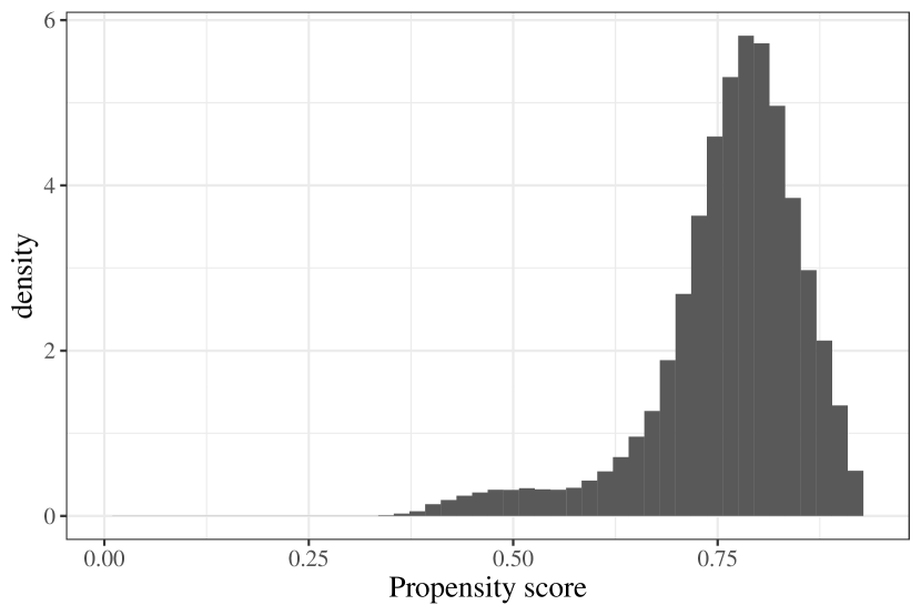
(a) No program

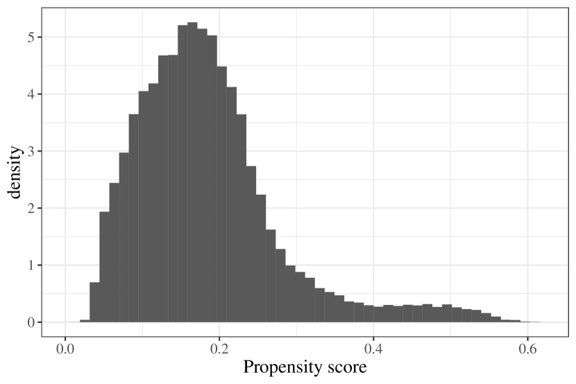
(b) Job search

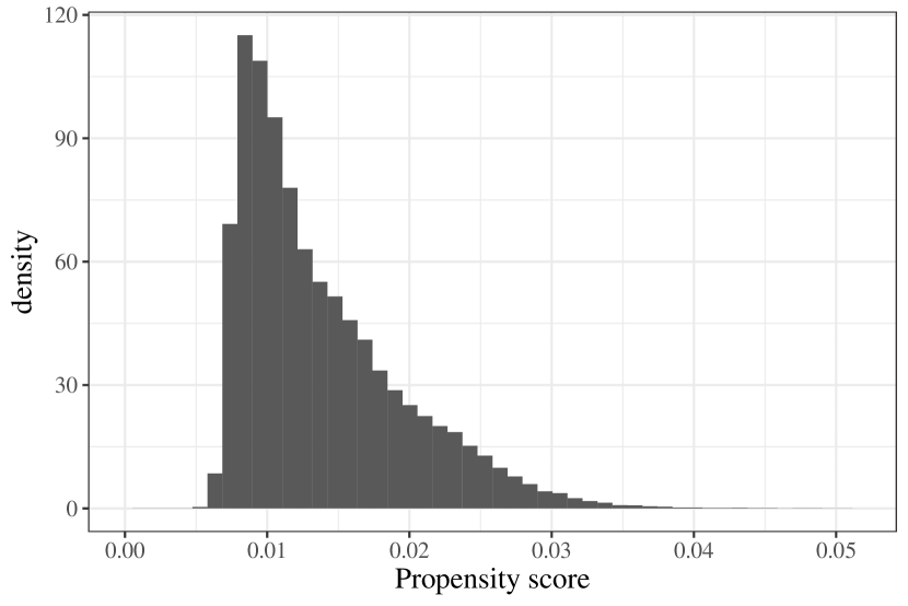
(c) Vocational

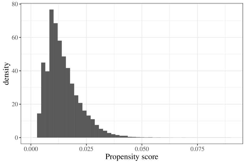
(d) Computer

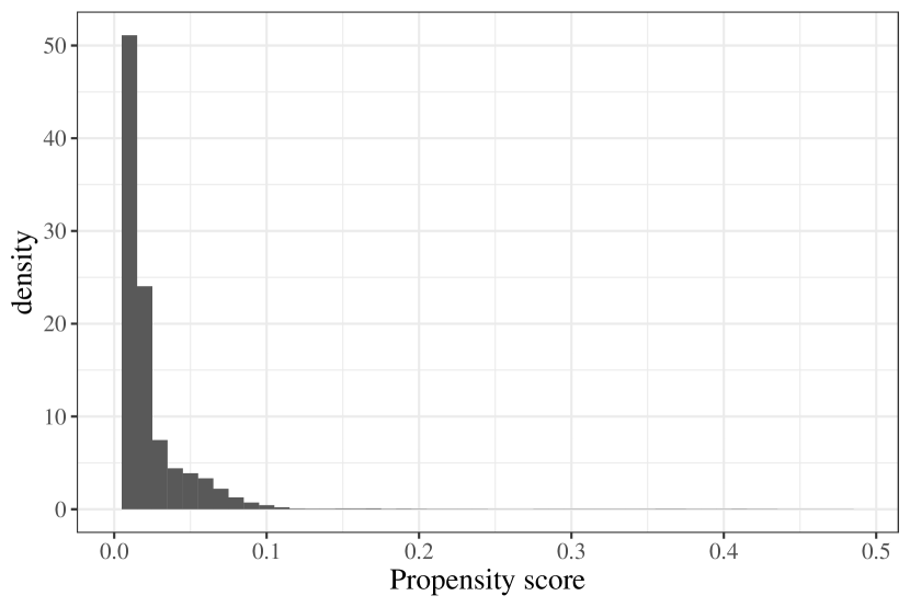
(e) Language

Table C.4: Summary statistics of propensity score distributions

	No program	Job search	Vocational	Computer	Language
Mean	0.764	0.184	0.014	0.015	0.024
SD	0.093	0.094	0.006	0.008	0.030
Minimum	0.321	0.027	0.005	0.003	0.005
Q1	0.439	0.045	0.007	0.004	0.006
Q25	0.727	0.120	0.009	0.009	0.009
Q50	0.779	0.170	0.012	0.013	0.015
Q75	0.824	0.224	0.017	0.018	0.025
Q99	0.910	0.515	0.031	0.038	0.109
Maximum	0.938	0.622	0.052	0.091	0.490

• Note: The table provides summary statistics of the program specific propensity score distributions. The rows denoted by Q show the respective quantiles.

C.3 Average treatment effects

Figure 2(a) shows the APO estimates and Figure 3(e) shows the effects of program participation on the employment probabilities over time. The latter documents that all program show the well-known lock-in effect within the first months after program start <e.g.>Wunsch2016HowWorkers. However, participants of the hard skill programs catch up and show a sustained increase in employment rates of up to 10 percentage points.

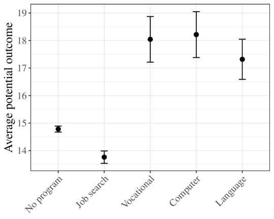
Figure C.2: Average potential outcomes

(a) Notes: Average potential outcomes with 95% confidence intervals. Numeric results in Panel A of Table C.5.

Figure C.3: Average treatment effects over time

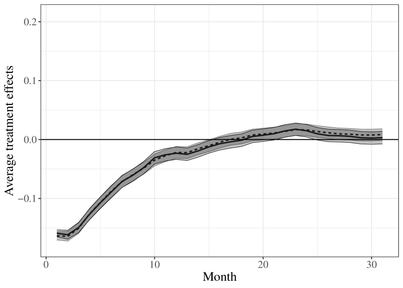
(a) Job search

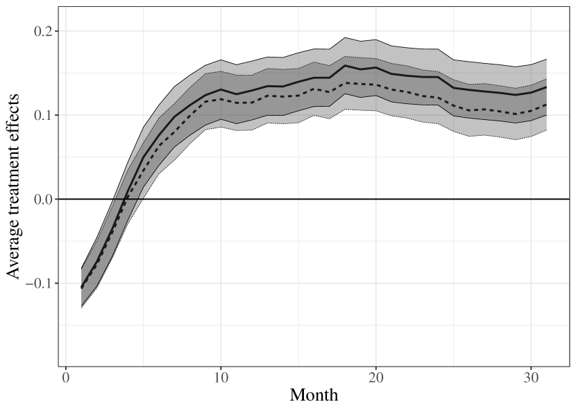
(b) Vocational

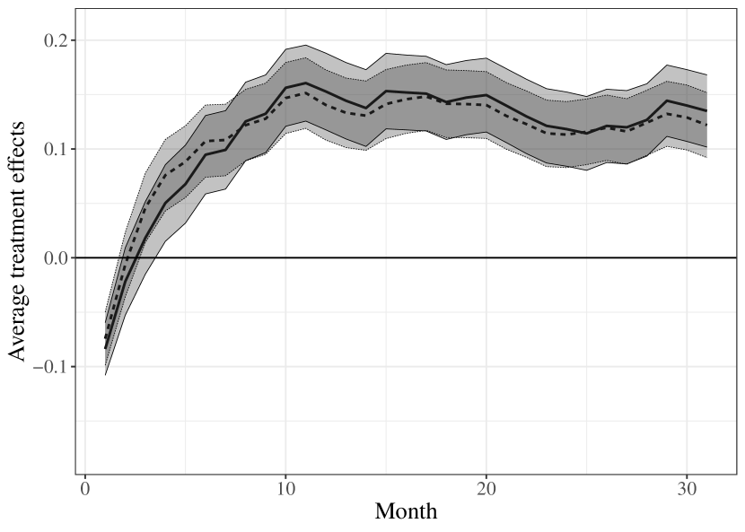
(c) Computer

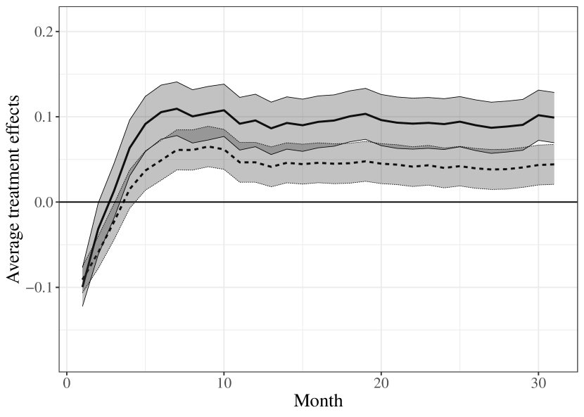
(d) Language

(e) Notes: Solid lines show ATE, dashed lines ATET of the respective programs compared to nonparticipation on employment probability in the 31 months after program start. Grey area depicts the 95% confidence intervals.

Table C.5: Average effects

	Estimate	Standard error
	(1)	(2)
Panel A: APO
No program	14.78	0.06
Job search	13.76	0.12
Vocational	18.04	0.42
Computer	18.21	0.43
Language	17.32	0.37
Panel B: ATE
Job search - no program	-1.02∗∗∗	0.13
Vocational - no program	3.26∗∗∗	0.43
Computer - no program	3.43∗∗∗	0.43
Language - no program	2.54∗∗∗	0.38
Panel C: ATET
Job search - no program	-0.98∗∗∗	0.12
Vocational - no program	2.79∗∗∗	0.39
Computer - no program	3.47∗∗∗	0.40
Language - no program	1.08∗∗∗	0.29

• Note: Table shows DML based point estimates and standard errors of average effects. ^∗p$<$0.1; ^∗∗p$<$0.05; ^∗∗∗p$<$0.01

C.4 GATEs

Figure 4(i) shows that the kernel and spline regressions detect no substantial heterogeneity for individuals of different age. All programs besides language courses show basically flat curves or at least the 95% confidence intervals includes the ATE. Only language courses show a larger positive effect for job seekers in the late twenties. Both kernel and spline regressions agree regarding this but the relatively erratic curves prevent deriving strong conclusions from these results.

Figure C.4: Effect heterogeneity regarding age

(a) Job search (Kernel)

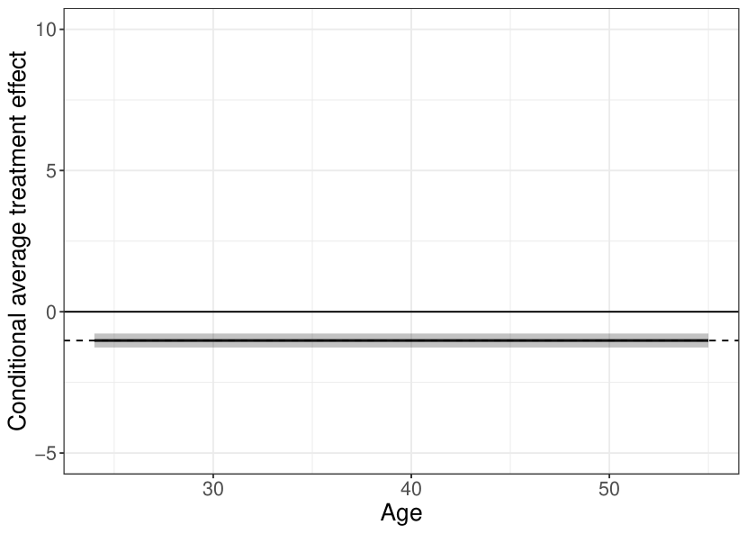
(b) Job search (Spline)

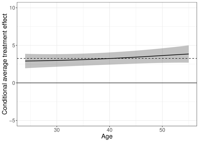
(c) Vocational (Kernel)

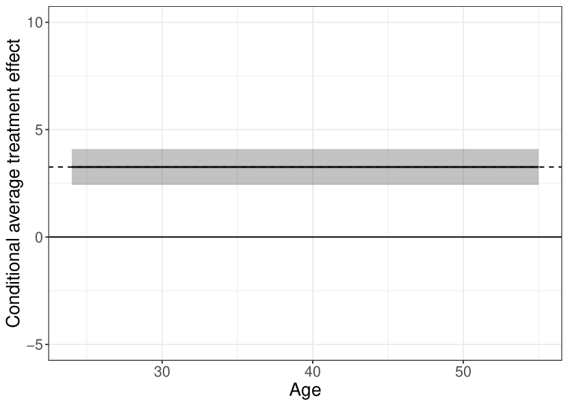
(d) Vocational (Spline)

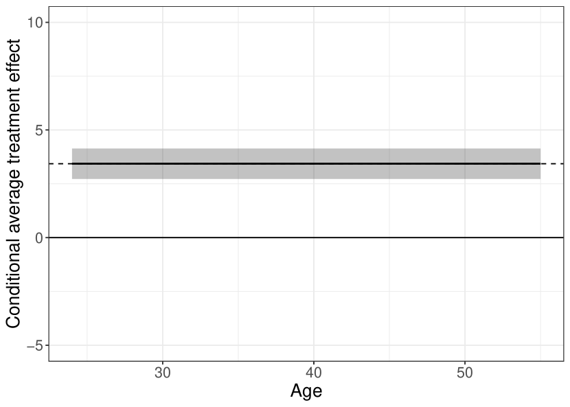
(e) Computer (Kernel)

(f) Computer (Spline)

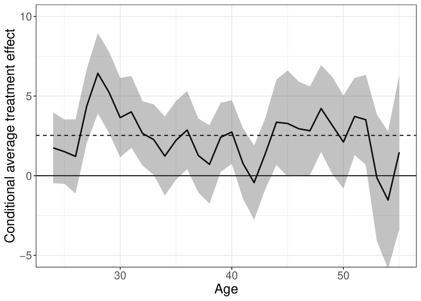
(g) Language (Kernel)

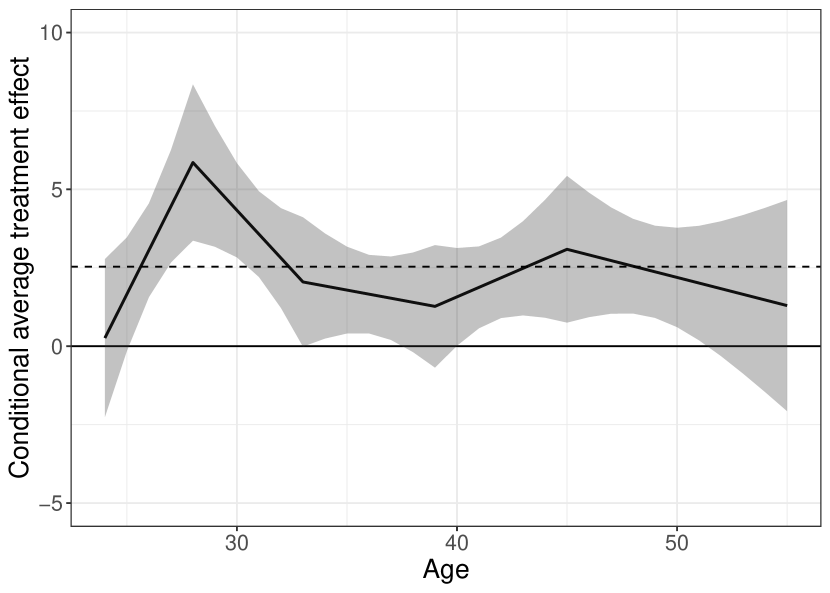
(h) Language (Spline)

(i) Dotted line indicates point estimate of the respective average treatment effect. Grey area shows 95%-confidence interval.

C.5 IATEs

Figure 5(a) documents the extreme IATE predictions obtained using the full sample. Especially the DR-learner produces very extreme estimates for vocational training ranging from -265 to 161. Also in this extreme case, the NDR-learner mitigates the problem substantially. However, Table C.6 documents that it still produces implausibly high values ranging from -19 to 20. The out-of-sample prediction of IATEs is thus preferred and discussed in the main text.

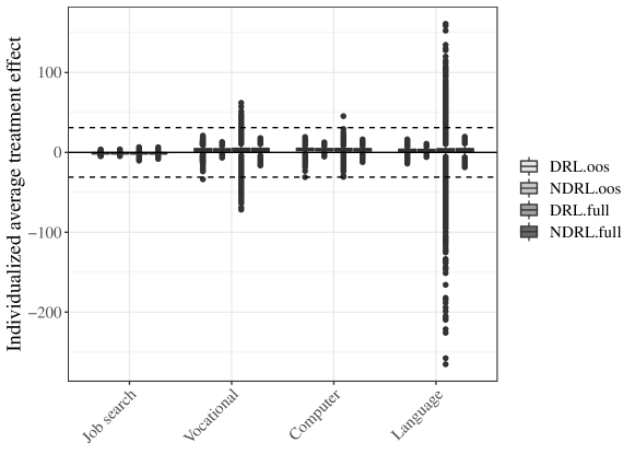
Figure C.5: Boxplot of IATEs estimated by DR- and NDR-learner

(a) Note: The figure shows the distribution of IATEs for participating in the program labeled on the x-axis vs. non-participation estimated by the DR-learner (DRL) and the NDR-learner (NDRL). The first two boxplots of a group are obtained using the out-of-sample (oos) procedure of Appendix B and the other two from the full sample. The dashed line indicates the possible range of the IATE of [-31,31] to illustrate that several DR-learner estimated IATEs lie outside this bound.

Table C.6 and Figure 6(e) provide a detailed comparison of the IATEs estimated by DR- and NDR-learner. We see that the differences are mainly driven by few outliers as indicated by the much larger kurtosis for the DR-learner IATEs. However, most of the estimates are quite similar as the correlations of at least 0.90 provided in the last row of panel A in Table C.6 and the scatter plots in Figure 6(e) document.

Table C.6: Summary statistics of IATE distributions

	Job search		Vocational		Computer		Language
	DRL	NDRL	DRL	NDRL	DRL	NDRL	DRL	NDRL
Panel A: Out-of-sample
Mean	-0.97	-0.99	3.17	3.13	3.68	3.54	2.55	2.50
SD	0.90	0.86	2.46	2.20	2.13	1.95	2.12	1.88
Minimum	-4.75	-4.68	-33.72	-6.71	-31.04	-5.33	-14.03	-5.79
Q1	-2.96	-2.91	-3.04	-2.14	-1.61	-1.01	-2.67	-1.95
Q25	-1.57	-1.57	1.65	1.68	2.34	2.25	1.24	1.21
Q50	-1.03	-1.04	3.22	3.14	3.69	3.51	2.57	2.57
Q75	-0.42	-0.45	4.77	4.58	5.04	4.80	3.85	3.80
Q99	1.34	1.22	8.78	8.36	8.65	8.31	7.90	6.74
Maximum	3.66	3.76	20.99	12.86	19.24	12.58	16.28	10.75
Kurtosis	3.35	3.35	5.63	3.22	6.37	3.28	4.28	2.98
Correlation	0.99		0.90		0.92		0.93
Panel B: Full sample
Mean	-1.03	-1.04	3.15	3.08	3.46	3.32	2.50	2.40
SD	1.20	1.14	4.07	3.03	2.31	2.17	7.51	3.42
Minimum	-10.42	-8.21	-71.74	-16.35	-30.67	-12.26	-265.23	-18.58
Q1	-3.89	-3.71	-6.18	-4.78	-2.06	-2.05	-11.07	-6.46
Q25	-1.80	-1.79	1.27	1.22	2.08	1.94	0.41	0.23
Q50	-1.07	-1.08	3.24	3.14	3.48	3.34	2.53	2.52
Q75	-0.29	-0.33	5.19	5.04	4.88	4.73	4.61	4.70
Q99	1.98	1.82	11.57	10.14	8.79	8.45	16.98	10.05
Maximum	6.53	6.45	62.01	17.92	45.33	16.30	160.92	19.63
Kurtosis	4.07	3.86	45.54	4.02	13.18	3.80	228.23	3.96
Correlation	0.99		0.86		0.94		0.67

• Note: The table provides summary statistics for the distributions of IATEs estimated by the DR-learner (DRL) and NDR-learner (NDRL). The rows denoted by Q show the respective quantiles. Correlation is calculated between the DR-learner and the NDR-learner. Bold numbers indicate values that are outside the possible range.

Figure C.6: Joint and marginal distributions of IATEs

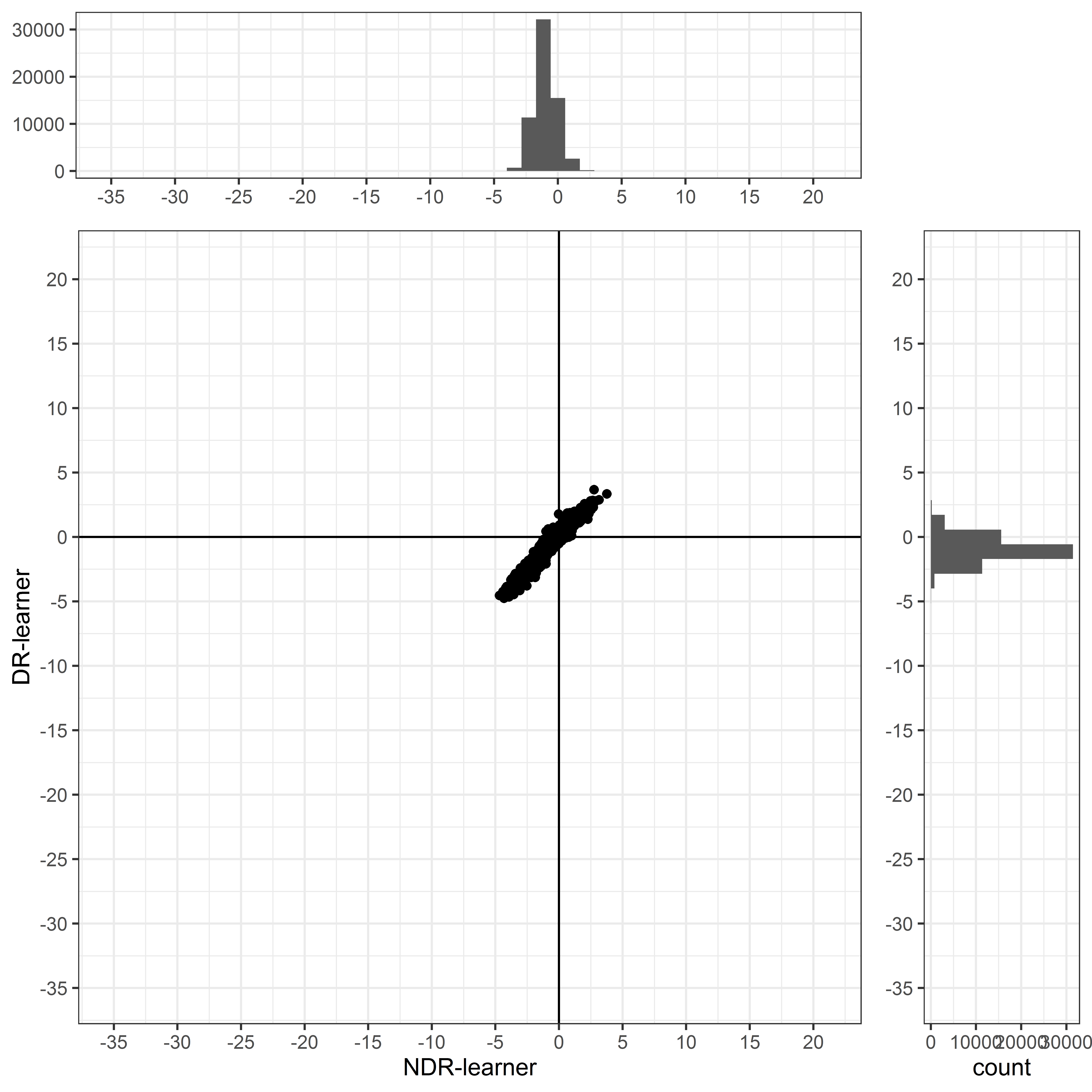
(a) Job search

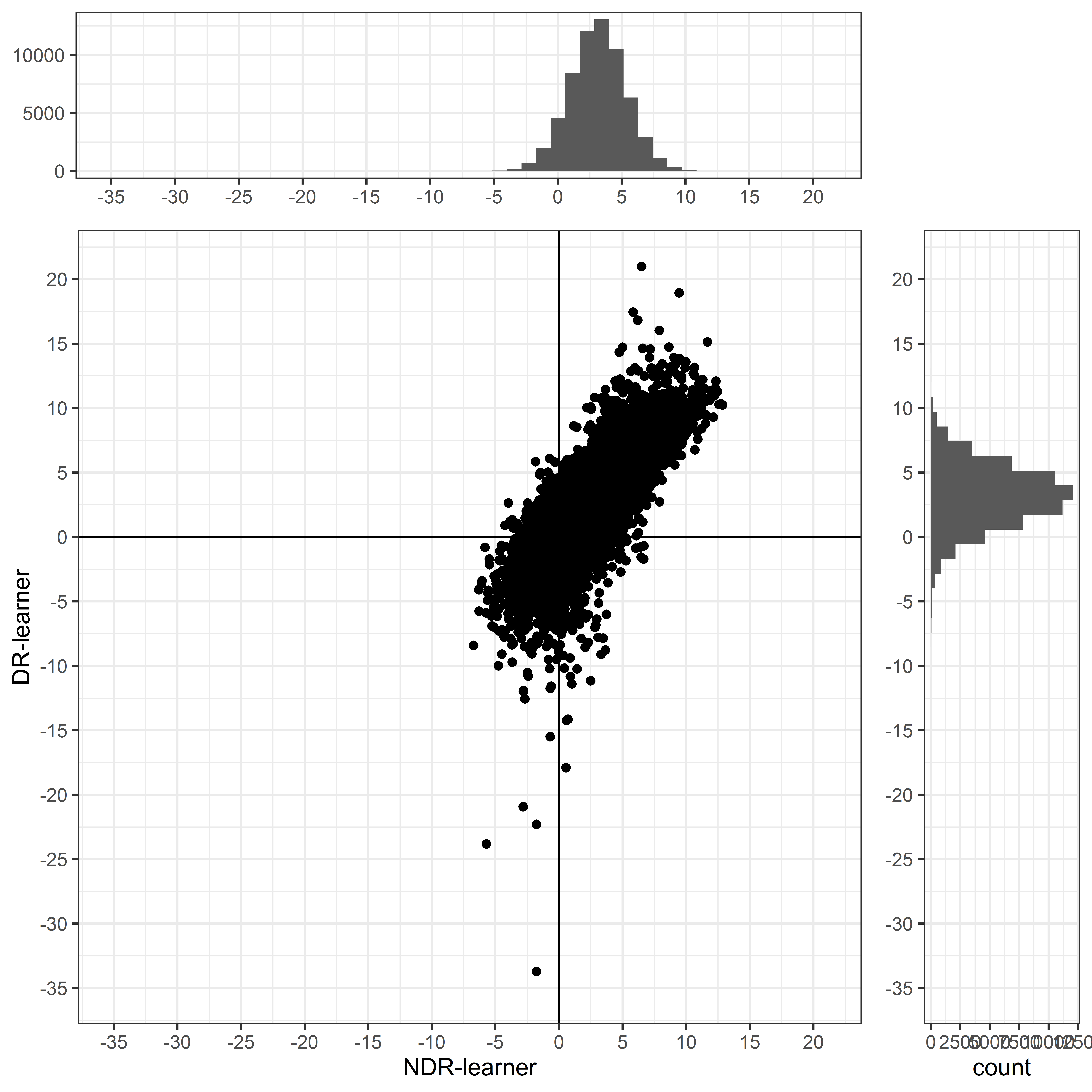
(b) Vocational

(c) Computer

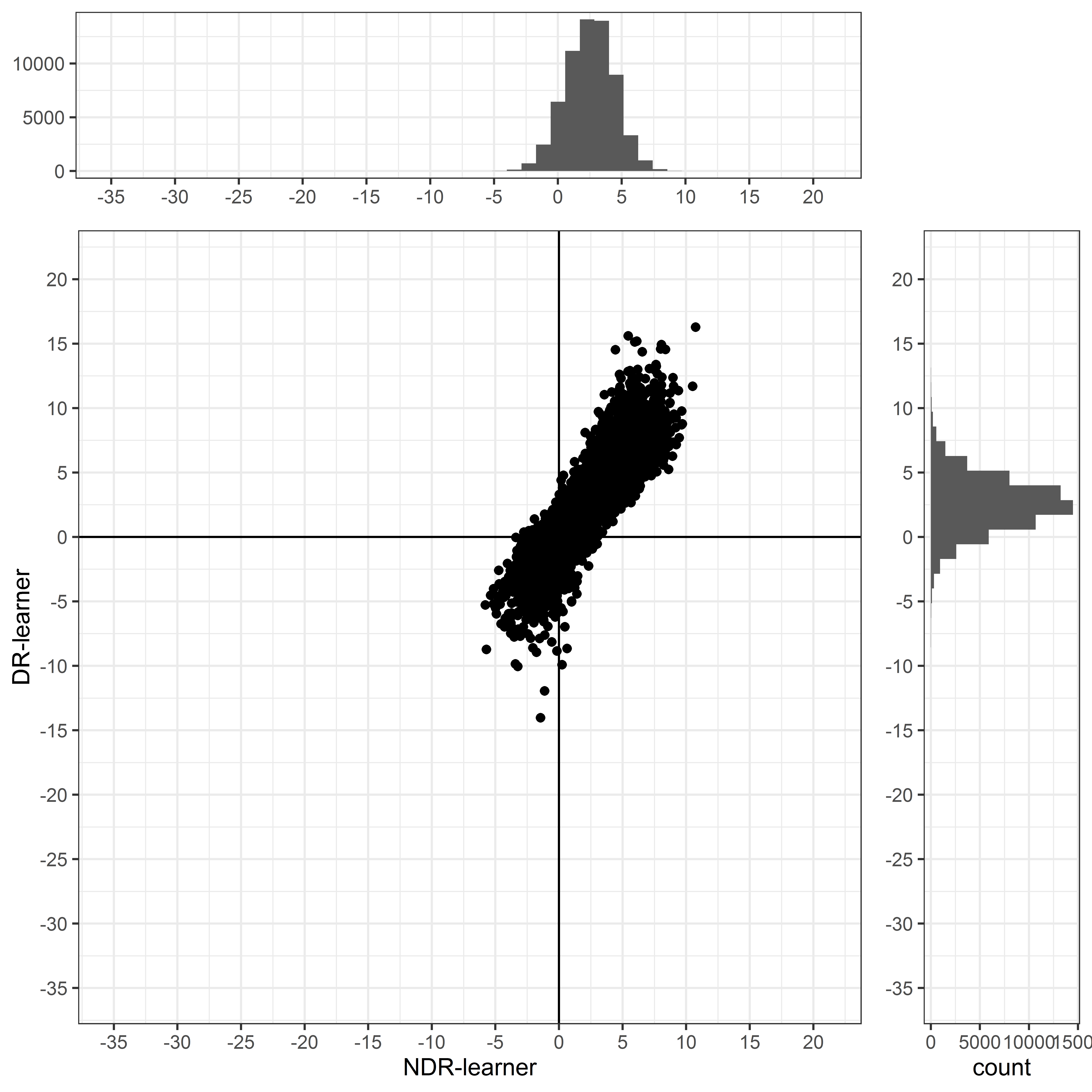
(d) Language

(e) Notes: Figures show the joint and marginal distributions of IATEs estimated by DR-learner and NDR-learner.

Table C.7 shows the full results of the classification analysis. In line with previous results of Knaus2020HeterogeneousApproach, we observe that the caseworker characteristics play a negligible role in explaining variation in IATEs. All caseworker related variables are in the lower half of the table.

[t]

Table C.7: Classification analysis of IATEs

	Job search	Vocational	Computer	Language
	(1)	(2)	(3)	(4)
Past income	-1.32	-0.84	-1.17	1.01
Previous job: unskilled worker	1.02	0.68	0.34	-1.24
Mother tongue other than German, French, Italian	0.69	0.68	0.00	-1.17
Qualification: some degree	-0.88	-0.65	-0.41	1.15
Swiss citizen	-0.66	-0.60	0.12	1.11
Fraction of months employed last 2 years	-1.06	-0.37	-0.47	0.30
Qualification: unskilled	0.81	0.41	0.32	-1.02
Previous job: skilled worker	-0.85	-0.41	-0.09	0.94
Missing sector	0.89	0.05	0.21	-0.53
Female	0.62	0.01	0.88	-0.48
Cantonal GDP p.c.	0.31	-0.78	0.01	0.26
Foreigner with temporary permit	0.55	0.35	0.09	-0.75
Cantonal unemployment rate (in %)	0.41	-0.72	0.02	0.13
Married	0.32	0.53	0.11	-0.69
Foreigner with permanent permit	0.31	0.40	-0.21	-0.67
Previous job in tertiary sector	-0.45	-0.31	0.03	0.58
Employability	-0.45	-0.55	-0.55	0.22
Number of employment spells last 5 years	0.53	0.22	0.04	-0.08
Number of unemployment spells last 2 years	0.47	0.11	0.13	-0.15
Previous job: manager	-0.27	-0.37	-0.36	0.40
Lives in no city	-0.40	0.26	0.10	0.06
Lives in big city	0.27	-0.38	-0.08	-0.09
Age	0.01	0.35	0.37	-0.01
Qualification: semiskilled	0.20	0.37	0.19	-0.30
Caseworker age	0.10	0.33	-0.00	0.08
Previous job in primary sector	-0.33	0.21	-0.28	-0.19
Allocation of unemployed to caseworkers: by occupation	0.17	0.02	0.23	0.30
Caseworker female	0.07	-0.26	0.29	-0.09
Allocation of unemployed to caseworkers: by region	-0.27	0.06	-0.05	-0.10
Lives in medium city	0.23	0.08	-0.04	0.03
Previous job in secondary sector	-0.10	0.22	-0.06	-0.07
Mother tongue in canton’s language	0.06	0.09	-0.18	-0.08
Qualification: skilled without degree	0.15	0.09	-0.00	-0.17
Caseworker education: above vocational training	-0.01	0.09	0.11	0.16
Caseworker education: tertiary track	0.00	-0.15	-0.12	-0.16
Caseworker cooperative	0.01	-0.06	0.15	-0.02
Allocation of unemployed to caseworkers: by employability	-0.12	0.10	0.02	0.05
Caseworker education: vocational degree	-0.12	-0.01	-0.11	-0.01
Caseworker tenure	0.04	0.02	-0.05	-0.10
Allocation of unemployed to caseworkers: by age	-0.05	0.00	0.10	0.04
Allocation of unemployed to caseworkers: by industry	0.10	-0.09	-0.02	-0.03
Missing caseworker characteristics	0.05	-0.09	0.05	-0.09
Previous job: self-employed	0.06	0.00	-0.02	0.03
Caseworker has own unemployemnt experience	0.03	-0.02	-0.04	0.06
Allocation of unemployed to caseworkers: other	-0.04	0.03	0.01	0.00

• Note: Table shows the differences in means of normalized covariates between the fifth and the first quintile of the respective estimated IATE distribution. Variables are ordered according to the largest absolute difference.

C.6 Optimal treatment assignment

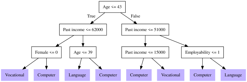
Figure C.7: Optimal decision tree of depth three with five covariates

Notes: Optimal assignment rules estimated following the procedure defined in Section 3.4.

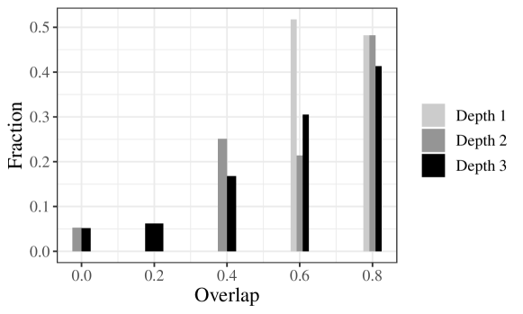
Figure C.8: Overlap of cross-validated policy rules with five covariates

Notes: Figure shows the fraction of cross-validated policies that agree with the full sample policy.

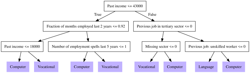
Figure C.9: Optimal decision tree of depth three with 16 covariates

Notes: Optimal assignment rules estimated following the procedure defined in Section 3.4.

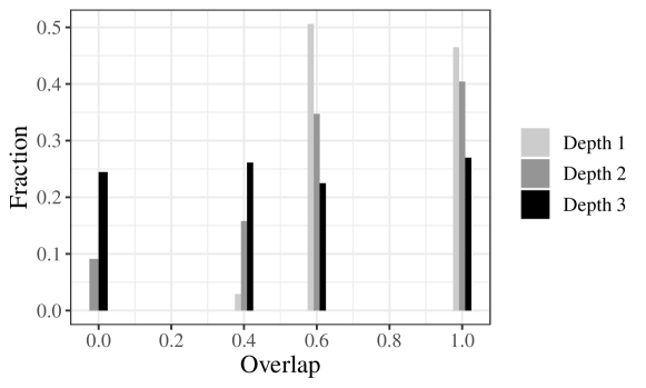
Figure C.10: Overlap of cross-validated policy rules with 16 covariates

Notes: Figure shows the fraction of cross-validated policies that agree with the full sample policy.

References

- Abadie \BBA Cattaneo (\APACyear2018) \APACinsertmetastarAbadie2018EconometricEvaluation{APACrefauthors}Abadie, A.\BCBT \BBA Cattaneo, M\BPBID. \APACrefYear2018. \BBOQ\APACrefatitleEconometric methods for program evaluation Econometric methods for program evaluation.\BBCQ \APACjournalVolNumPagesAnnual Review of Economics10465–503. \PrintBackRefs\CurrentBib
- Athey \BBA Imbens (\APACyear2019) \APACinsertmetastarAthey2019MachineAbout{APACrefauthors}Athey, S.\BCBT \BBA Imbens, G. \APACrefYear2019. \BBOQ\APACrefatitleMachine learning methods that economists should know about Machine learning methods that economists should know about.\BBCQ \APACjournalVolNumPagesAnnual Review of Economics11685–725. \PrintBackRefs\CurrentBib
- Athey \BBA Imbens (\APACyear2016) \APACinsertmetastarAthey2016{APACrefauthors}Athey, S.\BCBT \BBA Imbens, G\BPBIW. \APACrefYear2016. \BBOQ\APACrefatitleRecursive partitioning for heterogeneous causal effects Recursive partitioning for heterogeneous causal effects.\BBCQ \APACjournalVolNumPagesProceedings of the National Academy of Sciences113277353–7360. \PrintBackRefs\CurrentBib
- Athey \BBA Imbens (\APACyear2017) \APACinsertmetastarAthey2017{APACrefauthors}Athey, S.\BCBT \BBA Imbens, G\BPBIW. \APACrefYear2017. \BBOQ\APACrefatitleThe state of applied econometrics: causality and policy evaluation The state of applied econometrics: causality and policy evaluation.\BBCQ \APACjournalVolNumPagesJournal of Economic Perspectives3123–32. \PrintBackRefs\CurrentBib
- Athey \BOthers. (\APACyear2018) \APACinsertmetastarAthey2018ApproximateDimensions{APACrefauthors}Athey, S., Imbens, G\BPBIW.\BCBL \BBA Wager, S. \APACrefYear2018. \BBOQ\APACrefatitleApproximate residual balancing: Debiased inference of average treatment effects in high dimensions Approximate residual balancing: Debiased inference of average treatment effects in high dimensions.\BBCQ \APACjournalVolNumPagesJournal of the Royal Statistical Society: Series B (Statistical Methodology)804597–632. \PrintBackRefs\CurrentBib
- Athey \BOthers. (\APACyear2019) \APACinsertmetastarAthey2017a{APACrefauthors}Athey, S., Tibshirani, J.\BCBL \BBA Wager, S. \APACrefYear2019. \BBOQ\APACrefatitleGeneralized random forests Generalized random forests.\BBCQ \APACjournalVolNumPagesAnnals of Statistics4721148 - 1178. \PrintBackRefs\CurrentBib
- Athey \BBA Wager (\APACyear2021) \APACinsertmetastarAthey2021PolicyData{APACrefauthors}Athey, S.\BCBT \BBA Wager, S. \APACrefYear2021. \BBOQ\APACrefatitlePolicy learning with observational data Policy learning with observational data.\BBCQ \APACjournalVolNumPagesEconometrica891133–161. \PrintBackRefs\CurrentBib
- Avagyan \BBA Vansteelandt (\APACyear2017) \APACinsertmetastarAvagyan2017HonestEstimation{APACrefauthors}Avagyan, V.\BCBT \BBA Vansteelandt, S. \APACrefYear2017. \BBOQ\APACrefatitleHonest data-adaptive inference for the average treatment effect under model misspecification using penalised bias-reduced double-robust estimation Honest data-adaptive inference for the average treatment effect under model misspecification using penalised bias-reduced double-robust estimation.\BBCQ \APACjournalVolNumPagesarXiv:1708.03787. {APACrefURL} http://arxiv.org/abs/1708.03787 \PrintBackRefs\CurrentBib
- Baiardi \BBA Naghi (\APACyear2021) \APACinsertmetastarBaiardi2021TheStudies{APACrefauthors}Baiardi, A.\BCBT \BBA Naghi, A\BPBIA. \APACrefYear2021. \BBOQ\APACrefatitleThe value added of machine learning to causal inference: Evidence from revisited studies The value added of machine learning to causal inference: Evidence from revisited studies.\BBCQ \APACjournalVolNumPagesarXiv:2101.00878. \PrintBackRefs\CurrentBib
- Bansak \BOthers. (\APACyear2018) \APACinsertmetastarBansak2018ImprovingAssignment{APACrefauthors}Bansak, K., Ferwerda, J., Hainmueller, J., Dillon, A., Hangartner, D., Lawrence, D.\BCBL \BBA Weinstein, J. \APACrefYear2018. \BBOQ\APACrefatitleImproving refugee integration through data-driven algorithmic assignment Improving refugee integration through data-driven algorithmic assignment.\BBCQ \APACjournalVolNumPagesScience3596373325–329. \PrintBackRefs\CurrentBib
- Belloni \BBA Chernozhukov (\APACyear2013) \APACinsertmetastarBelloni2013LeastModels{APACrefauthors}Belloni, A.\BCBT \BBA Chernozhukov, V. \APACrefYear2013. \BBOQ\APACrefatitleLeast squares after model selection in high-dimensional sparse models Least squares after model selection in high-dimensional sparse models.\BBCQ \APACjournalVolNumPagesBernoulli192521–547. \PrintBackRefs\CurrentBib
- Belloni \BOthers. (\APACyear2017) \APACinsertmetastarBelloni2017{APACrefauthors}Belloni, A., Chernozhukov, V., Fernández-Val, I.\BCBL \BBA Hansen, C. \APACrefYear2017. \BBOQ\APACrefatitleProgram evaluation and causal inference with high-dimensional data Program evaluation and causal inference with high-dimensional data.\BBCQ \APACjournalVolNumPagesEconometrica851233–298. \PrintBackRefs\CurrentBib
- Belloni \BOthers. (\APACyear2014) \APACinsertmetastarBelloni2014InferenceControls{APACrefauthors}Belloni, A., Chernozhukov, V.\BCBL \BBA Hansen, C. \APACrefYear2014. \BBOQ\APACrefatitleInference on treatment effects after selection among high-dimensional controls Inference on treatment effects after selection among high-dimensional controls.\BBCQ \APACjournalVolNumPagesReview of Economic Studies812608–650. \PrintBackRefs\CurrentBib
- Bertrand \BOthers. (\APACyear2017) \APACinsertmetastarBertrand2017{APACrefauthors}Bertrand, M., Crépon, B., Marguerie, A.\BCBL \BBA Premand, P. \APACrefYear2017. \BBOQ\APACrefatitleContemporaneous and post-program impacts of a public works program: Evidence from Côte d’Ivoire Contemporaneous and post-program impacts of a public works program: Evidence from Côte d’Ivoire.\BBCQ \APACjournalVolNumPagesWorld Bank Working Paper. \PrintBackRefs\CurrentBib
- Breiman (\APACyear2001) \APACinsertmetastarBreiman2001{APACrefauthors}Breiman, L. \APACrefYear2001. \BBOQ\APACrefatitleRandom forests Random forests.\BBCQ \APACjournalVolNumPagesMachine Learning4515–32. \PrintBackRefs\CurrentBib
- Buja \BOthers. (\APACyear1989) \APACinsertmetastarBuja1989LinearModels{APACrefauthors}Buja, A., Hastie, T.\BCBL \BBA Tibshirani, R. \APACrefYear1989. \BBOQ\APACrefatitleLinear smoothers and additive models Linear smoothers and additive models.\BBCQ \APACjournalVolNumPagesThe Annals of Statistics172453–510. \PrintBackRefs\CurrentBib
- Busso \BOthers. (\APACyear2014) \APACinsertmetastarbusso2014new{APACrefauthors}Busso, M., DiNardo, J.\BCBL \BBA McCrary, J. \APACrefYear2014. \BBOQ\APACrefatitleNew evidence on the finite sample properties of propensity score reweighting and matching estimators New evidence on the finite sample properties of propensity score reweighting and matching estimators.\BBCQ \APACjournalVolNumPagesReview of Economics and Statistics965885–897. \PrintBackRefs\CurrentBib
- Card \BOthers. (\APACyear2018) \APACinsertmetastarCard2018WhatEvaluations{APACrefauthors}Card, D., Kluve, J.\BCBL \BBA Weber, A. \APACrefYear2018. \BBOQ\APACrefatitleWhat works? A meta analysis of recent active labor market program evaluations What works? A meta analysis of recent active labor market program evaluations.\BBCQ \APACjournalVolNumPagesJournal of the European Economic Association163894–931. \PrintBackRefs\CurrentBib
- Chernozhukov, Chetverikov\BCBL \BOthers. (\APACyear2018) \APACinsertmetastarChernozhukov2018{APACrefauthors}Chernozhukov, V., Chetverikov, D., Demirer, M., Duflo, E., Hansen, C., Newey, W.\BCBL \BBA Robins, J. \APACrefYear2018. \BBOQ\APACrefatitleDouble/Debiased machine learning for treatment and structural parameters Double/Debiased machine learning for treatment and structural parameters.\BBCQ \APACjournalVolNumPagesThe Econometrics Journal211C1-C68. \PrintBackRefs\CurrentBib
- Chernozhukov \BOthers. (\APACyear2017) \APACinsertmetastarChernozhukov2017GenericExperiments{APACrefauthors}Chernozhukov, V., Demirer, M., Duflo, E.\BCBL \BBA Fernandez-Val, I. \APACrefYear2017. \BBOQ\APACrefatitleGeneric machine learning inference on heterogenous treatment effects in randomized experiments Generic machine learning inference on heterogenous treatment effects in randomized experiments.\BBCQ \APACjournalVolNumPagesarXiv:1712.04802. {APACrefURL} http://arxiv.org/abs/1712.04802 \PrintBackRefs\CurrentBib
- Chernozhukov, Fernandez-Val\BCBL \BBA Luo (\APACyear2018) \APACinsertmetastarChernozhukov2018TheAverages{APACrefauthors}Chernozhukov, V., Fernandez-Val, I.\BCBL \BBA Luo, Y. \APACrefYear2018. \BBOQ\APACrefatitleThe sorted effects method: Discovering heterogeneous effects beyond their averages The sorted effects method: Discovering heterogeneous effects beyond their averages.\BBCQ \APACjournalVolNumPagesEconometrica8661911–1938. \PrintBackRefs\CurrentBib
- Cockx \BOthers. (\APACyear2020) \APACinsertmetastarCockx2020PriorityBelgium{APACrefauthors}Cockx, B., Lechner, M.\BCBL \BBA Bollens, J. \APACrefYear2020. \BBOQ\APACrefatitlePriority to unemployed immigrants? A causal machine learning evaluation of training in Belgium Priority to unemployed immigrants? A causal machine learning evaluation of training in Belgium.\BBCQ \APACjournalVolNumPagesCEPR Discussion Paper No. DP14270. \PrintBackRefs\CurrentBib
- Colangelo \BBA Lee (\APACyear2019) \APACinsertmetastarColangelo2019DoubleTreatments{APACrefauthors}Colangelo, K.\BCBT \BBA Lee, Y\BHBIY. \APACrefYear2019. \BBOQ\APACrefatitleDouble debiased machine learning nonparametric inference with continuous treatments Double debiased machine learning nonparametric inference with continuous treatments.\BBCQ \APACjournalVolNumPagesarXiv:2004.03036. \PrintBackRefs\CurrentBib
- Crépon \BBA van den Berg (\APACyear2016) \APACinsertmetastarcrepon2016active{APACrefauthors}Crépon, B.\BCBT \BBA van den Berg, G\BPBIJ. \APACrefYear2016. \BBOQ\APACrefatitleActive labor market policies Active labor market policies.\BBCQ \APACjournalVolNumPagesAnnual Review of Economics8521–546. \PrintBackRefs\CurrentBib
- Curth \BBA van der Schaar (\APACyear2021) \APACinsertmetastarCurth2021NonparametricAlgorithms{APACrefauthors}Curth, A.\BCBT \BBA van der Schaar, M. \APACrefYear2021. \BBOQ\APACrefatitleNonparametric estimation of heterogeneous treatment effects: From theory to learning algorithms Nonparametric estimation of heterogeneous treatment effects: From theory to learning algorithms.\BBCQ \BIn \APACrefbtitleProceedings of The 24th International Conference on Artificial Intelligence and Statistics Proceedings of the 24th international conference on artificial intelligence and statistics (\BVOL 130, \BPGS 1810–1818). \APACaddressPublisherPMLR. \PrintBackRefs\CurrentBib
- Davis \BBA Heller (\APACyear2020) \APACinsertmetastarDavis2020RethinkingJobs{APACrefauthors}Davis, J\BPBIM\BPBIV.\BCBT \BBA Heller, S\BPBIB. \APACrefYear2020. \BBOQ\APACrefatitleRethinking the benefits of youth employment programs: The heterogeneous effects of summer jobs Rethinking the benefits of youth employment programs: The heterogeneous effects of summer jobs.\BBCQ \APACjournalVolNumPagesThe Review of Economics and Statistics1024664–677. \PrintBackRefs\CurrentBib
- Dudik \BOthers. (\APACyear2011) \APACinsertmetastarDudik2011DoublyLearning{APACrefauthors}Dudik, M., Langford, J.\BCBL \BBA Li, L. \APACrefYear2011. \BBOQ\APACrefatitleDoubly robust policy evaluation and learning Doubly robust policy evaluation and learning.\BBCQ \APACjournalVolNumPagesarXiv:1103.4601. {APACrefURL} http://arxiv.org/abs/1103.4601 \PrintBackRefs\CurrentBib
- Fan \BOthers. (\APACyear2020) \APACinsertmetastarfan2020EstimationData{APACrefauthors}Fan, Q., Hsu, Y\BHBIC., Lieli, R\BPBIP.\BCBL \BBA Zhang, Y. \APACrefYear2020. \BBOQ\APACrefatitleEstimation of conditional average treatment effects with high-dimensional data Estimation of conditional average treatment effects with high-dimensional data.\BBCQ \APACjournalVolNumPagesJournal of Business & Economic Statisticspublished ahead of print 14 September 2020. \PrintBackRefs\CurrentBib
- Farbmacher \BOthers. (\APACyear2021) \APACinsertmetastarFarbmacher2021HeterogeneousCognition{APACrefauthors}Farbmacher, H., Kögel, H.\BCBL \BBA Spindler, M. \APACrefYear2021. \BBOQ\APACrefatitleHeterogeneous effects of poverty on cognition Heterogeneous effects of poverty on cognition.\BBCQ \APACjournalVolNumPagesLabour Economics71102028. \PrintBackRefs\CurrentBib
- Farrell (\APACyear2015) \APACinsertmetastarFarrell2015{APACrefauthors}Farrell, M\BPBIH. \APACrefYear2015. \BBOQ\APACrefatitleRobust inference on average treatment effects with possibly more covariates than observations Robust inference on average treatment effects with possibly more covariates than observations.\BBCQ \APACjournalVolNumPagesJournal of Econometrics18911–23. \PrintBackRefs\CurrentBib
- Farrell \BOthers. (\APACyear2021) \APACinsertmetastarFarrell2021DeepInference{APACrefauthors}Farrell, M\BPBIH., Liang, T.\BCBL \BBA Misra, S. \APACrefYear2021. \BBOQ\APACrefatitleDeep neural networks for estimation and inference Deep neural networks for estimation and inference.\BBCQ \APACjournalVolNumPagesEconometrica891181–213. \PrintBackRefs\CurrentBib
- Foster \BBA Syrgkanis (\APACyear2019) \APACinsertmetastarFoster2019OrthogonalLearning{APACrefauthors}Foster, D\BPBIJ.\BCBT \BBA Syrgkanis, V. \APACrefYear2019. \BBOQ\APACrefatitleOrthogonal statistical learning Orthogonal statistical learning.\BBCQ \APACjournalVolNumPagesarXiv:1901.09036. {APACrefURL} http://arxiv.org/abs/1901.09036 \PrintBackRefs\CurrentBib
- Gerfin \BBA Lechner (\APACyear2002) \APACinsertmetastargerfin2002microeconometric{APACrefauthors}Gerfin, M.\BCBT \BBA Lechner, M. \APACrefYear2002. \BBOQ\APACrefatitleA microeconometric evaluation of the active labour market policy in Switzerland A microeconometric evaluation of the active labour market policy in Switzerland.\BBCQ \APACjournalVolNumPagesEconomic Journal112482854–893. \PrintBackRefs\CurrentBib
- Glynn \BBA Quinn (\APACyear2009) \APACinsertmetastarGlynn2009AnEstimator{APACrefauthors}Glynn, A\BPBIN.\BCBT \BBA Quinn, K\BPBIM. \APACrefYear2009. \BBOQ\APACrefatitleAn introduction to the augmented inverse propensity weighted estimator An introduction to the augmented inverse propensity weighted estimator.\BBCQ \APACjournalVolNumPagesPolitical Analysis18136–56. \PrintBackRefs\CurrentBib
- Gulyas \BBA Pytka (\APACyear2019) \APACinsertmetastarGulyas2019UnderstandingApproach{APACrefauthors}Gulyas, A.\BCBT \BBA Pytka, K. \APACrefYear2019. \BBOQ\APACrefatitleUnderstanding the sources of earnings losses after job displacement: A machine-learning approach Understanding the sources of earnings losses after job displacement: A machine-learning approach.\BBCQ \APACjournalVolNumPagesDiscussion Paper Series – CRC TR 224 No. 131. \PrintBackRefs\CurrentBib
- Hájek (\APACyear1971) \APACinsertmetastarHajek1971CommentOne{APACrefauthors}Hájek, J. \APACrefYear1971. \BBOQ\APACrefatitleComment on “An essay on the logical foundations of survey sampling, part one” Comment on “An essay on the logical foundations of survey sampling, part one”.\BBCQ \BIn V\BPBIP. Godambe \BBA D\BPBIA. Sprott (\BEDS), \APACrefbtitleFoundations of Statistical Inference Foundations of statistical inference (\BPG 236). \APACaddressPublisherTorontoHolt, Rinehart and Winston. \PrintBackRefs\CurrentBib
- Hayfield \BBA Racine (\APACyear2008) \APACinsertmetastarHayfield2008NonparametricPackage{APACrefauthors}Hayfield, T.\BCBT \BBA Racine, J\BPBIS. \APACrefYear2008. \BBOQ\APACrefatitleNonparametric econometrics: The np package Nonparametric econometrics: The np package.\BBCQ \APACjournalVolNumPagesJournal of Statistical Software275. \PrintBackRefs\CurrentBib
- Heiler \BBA Knaus (\APACyear2021) \APACinsertmetastarHeiler2021EffectTreatments{APACrefauthors}Heiler, P.\BCBT \BBA Knaus, M\BPBIC. \APACrefYear2021. \BBOQ\APACrefatitleEffect or treatment heterogeneity? Policy evaluation with aggregated and disaggregated treatments Effect or treatment heterogeneity? Policy evaluation with aggregated and disaggregated treatments.\BBCQ \APACjournalVolNumPagesarXiv:2110.01427. {APACrefURL} http://arxiv.org/abs/2110.01427 \PrintBackRefs\CurrentBib
- Hirano \BBA Porter (\APACyear2009) \APACinsertmetastarHirano2009AsymptoticsRules{APACrefauthors}Hirano, K.\BCBT \BBA Porter, J\BPBIR. \APACrefYear2009. \BBOQ\APACrefatitleAsymptotics for statistical treatment rules Asymptotics for statistical treatment rules.\BBCQ \APACjournalVolNumPagesEconometrica7751683–1701. \PrintBackRefs\CurrentBib
- Holland (\APACyear1986) \APACinsertmetastarHolland1986StatisticsInference{APACrefauthors}Holland, P\BPBIW. \APACrefYear1986. \BBOQ\APACrefatitleStatistics and causal inference Statistics and causal inference.\BBCQ \APACjournalVolNumPagesJournal of the American Statistical Association81396945–960. \PrintBackRefs\CurrentBib
- Huber \BOthers. (\APACyear2017) \APACinsertmetastarHuber2017{APACrefauthors}Huber, M., Lechner, M.\BCBL \BBA Mellace, G. \APACrefYear2017. \BBOQ\APACrefatitleWhy do tougher caseworkers increase employment? The role of program assignment as a causal mechanism Why do tougher caseworkers increase employment? The role of program assignment as a causal mechanism.\BBCQ \APACjournalVolNumPagesReview of Economics and Statistics991180–183. \PrintBackRefs\CurrentBib
- Imbens (\APACyear2000) \APACinsertmetastarImbens2000TheFunctions{APACrefauthors}Imbens, G\BPBIW. \APACrefYear2000. \BBOQ\APACrefatitleThe role of the propensity score in estimating dose-response functions The role of the propensity score in estimating dose-response functions.\BBCQ \APACjournalVolNumPagesBiometrika873706–710. \PrintBackRefs\CurrentBib
- Imbens (\APACyear2004) \APACinsertmetastarImbens2004NonparametricReview{APACrefauthors}Imbens, G\BPBIW. \APACrefYear2004. \BBOQ\APACrefatitleNonparametric estimation of average treatment effects under exogeneity: A review Nonparametric estimation of average treatment effects under exogeneity: A review.\BBCQ \APACjournalVolNumPagesReview of Economics and Statistics8614–29. \PrintBackRefs\CurrentBib
- Imbens \BBA Rubin (\APACyear2015) \APACinsertmetastarImbens2015CausalSciences{APACrefauthors}Imbens, G\BPBIW.\BCBT \BBA Rubin, D\BPBIB. \APACrefYear2015. \APACrefbtitleCausal inference in statistics, social, and biomedical sciences Causal inference in statistics, social, and biomedical sciences. \APACaddressPublisherCambridge University Press. \PrintBackRefs\CurrentBib
- Isphording (\APACyear2014) \APACinsertmetastarIsphording2014LanguageSuccess{APACrefauthors}Isphording, I\BPBIE. \APACrefYear2014. \BBOQ\APACrefatitleLanguage and labor market success Language and labor market success.\BBCQ \APACjournalVolNumPagesIZA Discussion Papers No. 85728572. \PrintBackRefs\CurrentBib
- Kallus (\APACyear2018) \APACinsertmetastarKallus2018BalancedLearning{APACrefauthors}Kallus, N. \APACrefYear2018. \BBOQ\APACrefatitleBalanced policy evaluation and learning Balanced policy evaluation and learning.\BBCQ \BIn \APACrefbtitleAdvances in Neural Information Processing Systems Advances in neural information processing systems (\BPGS 8895–8906). \PrintBackRefs\CurrentBib
- Kallus \BOthers. (\APACyear2019) \APACinsertmetastarKallus2019LocalizedBeyond{APACrefauthors}Kallus, N., Mao, X.\BCBL \BBA Uehara, M. \APACrefYear2019. \BBOQ\APACrefatitleLocalized Debiased Machine Learning: Efficient Estimation of Quantile Treatment Effects, Conditional Value at Risk, and Beyond Localized Debiased Machine Learning: Efficient Estimation of Quantile Treatment Effects, Conditional Value at Risk, and Beyond.\BBCQ \APACjournalVolNumPagesarXiv:1912.12945. {APACrefURL} http://arxiv.org/abs/1912.12945 \PrintBackRefs\CurrentBib
- Kang \BBA Schafer (\APACyear2007) \APACinsertmetastarKang2007{APACrefauthors}Kang, J\BPBID\BPBIY.\BCBT \BBA Schafer, J\BPBIL. \APACrefYear2007. \BBOQ\APACrefatitleDemystifying double robustness: A comparison of alternative strategies for estimating a population mean from incomplete data Demystifying double robustness: A comparison of alternative strategies for estimating a population mean from incomplete data.\BBCQ \APACjournalVolNumPagesStatistical Science224523–539. \PrintBackRefs\CurrentBib
- Kennedy (\APACyear2020) \APACinsertmetastarKennedy2020OptimalEffects{APACrefauthors}Kennedy, E\BPBIH. \APACrefYear2020. \BBOQ\APACrefatitleOptimal doubly robust estimation of heterogeneous causal effects Optimal doubly robust estimation of heterogeneous causal effects.\BBCQ \APACjournalVolNumPagesarXiv:2004.14497. {APACrefURL} http://arxiv.org/abs/2004.14497 \PrintBackRefs\CurrentBib
- Kennedy \BOthers. (\APACyear2017) \APACinsertmetastarKennedy2017Non-parametricEffects{APACrefauthors}Kennedy, E\BPBIH., Ma, Z., McHugh, M\BPBID.\BCBL \BBA Small, D\BPBIS. \APACrefYear2017. \BBOQ\APACrefatitleNon-parametric methods for doubly robust estimation of continuous treatment effects Non-parametric methods for doubly robust estimation of continuous treatment effects.\BBCQ \APACjournalVolNumPagesJournal of the Royal Statistical Society: Series B (Statistical Methodology)791229–1245. \PrintBackRefs\CurrentBib
- Kitagawa \BBA Tetenov (\APACyear2018) \APACinsertmetastarKitagawa2018WhoChoice{APACrefauthors}Kitagawa, T.\BCBT \BBA Tetenov, A. \APACrefYear2018. \BBOQ\APACrefatitleWho should be treated? Empirical welfare maximization methods for treatment choice Who should be treated? Empirical welfare maximization methods for treatment choice.\BBCQ \APACjournalVolNumPagesEconometrica862591–616. \PrintBackRefs\CurrentBib
- Knaus (\APACyear2021) \APACinsertmetastarKnaus2021ASkills{APACrefauthors}Knaus, M\BPBIC. \APACrefYear2021. \BBOQ\APACrefatitleA double machine learning approach to estimate the effects of musical practice on student’s skills A double machine learning approach to estimate the effects of musical practice on student’s skills.\BBCQ \APACjournalVolNumPagesJournal of the Royal Statistical Society. Series A: Statistics in Society1841282–300. \PrintBackRefs\CurrentBib
- Knaus \BOthers. (\APACyear2020) \APACinsertmetastarKnaus2020HeterogeneousApproach{APACrefauthors}Knaus, M\BPBIC., Lechner, M.\BCBL \BBA Strittmatter, A. \APACrefYear2020. \BBOQ\APACrefatitleHeterogeneous employment effects of job search programmes: A machine learning approach Heterogeneous employment effects of job search programmes: A machine learning approach.\BBCQ \APACjournalVolNumPagesJournal of Human Resources0718-9615Rpublished ahead of print 26 March 2020. \PrintBackRefs\CurrentBib
- Knaus \BOthers. (\APACyear2021) \APACinsertmetastarKnaus2021{APACrefauthors}Knaus, M\BPBIC., Lechner, M.\BCBL \BBA Strittmatter, A. \APACrefYear2021. \BBOQ\APACrefatitleMachine Learning Estimation of Heterogeneous Causal Effects: Empirical Monte Carlo Evidence Machine Learning Estimation of Heterogeneous Causal Effects: Empirical Monte Carlo Evidence.\BBCQ \APACjournalVolNumPagesThe Econometrics Journal241134–161. \PrintBackRefs\CurrentBib
- Knittel \BBA Stolper (\APACyear2019) \APACinsertmetastarKnittel2019UsingUse{APACrefauthors}Knittel, C\BPBIR.\BCBT \BBA Stolper, S. \APACrefYear2019. \BBOQ\APACrefatitleUsing machine learning to target treatment: The case of household energy use Using machine learning to target treatment: The case of household energy use.\BBCQ \APACjournalVolNumPagesNBER Working Paper No. 26531. \PrintBackRefs\CurrentBib
- Kozbur (\APACyear2020) \APACinsertmetastarKozbur2020AnalysisSelection{APACrefauthors}Kozbur, D. \APACrefYear2020. \BBOQ\APACrefatitleAnalysis of testing-based forward model selection Analysis of testing-based forward model selection.\BBCQ \APACjournalVolNumPagesEconometrica8852147–2173. \PrintBackRefs\CurrentBib
- Kreif \BBA DiazOrdaz (\APACyear2019) \APACinsertmetastarKreif2019MachineInference{APACrefauthors}Kreif, N.\BCBT \BBA DiazOrdaz, K. \APACrefYear2019. \BBOQ\APACrefatitleMachine learning in policy evaluation: new tools for causal inference Machine learning in policy evaluation: new tools for causal inference.\BBCQ \APACjournalVolNumPagesarXiv:1903.00402. {APACrefURL} http://arxiv.org/abs/1903.00402 \PrintBackRefs\CurrentBib
- Künzel \BOthers. (\APACyear2019) \APACinsertmetastarKunzel2017{APACrefauthors}Künzel, S\BPBIR., Sekhon, J\BPBIS., Bickel, P\BPBIJ.\BCBL \BBA Yu, B. \APACrefYear2019. \BBOQ\APACrefatitleMetalearners for estimating heterogeneous treatment effects using machine learning Metalearners for estimating heterogeneous treatment effects using machine learning.\BBCQ \APACjournalVolNumPagesProceedings of the National Academy of Sciences116104156–4165. \PrintBackRefs\CurrentBib
- Lalive \BOthers. (\APACyear2008) \APACinsertmetastarLalive2008TheUnemployment{APACrefauthors}Lalive, R., van Ours, J.\BCBL \BBA Zweimüller, J. \APACrefYear2008. \BBOQ\APACrefatitleThe impact of active labor market programs on the duration of unemployment The impact of active labor market programs on the duration of unemployment.\BBCQ \APACjournalVolNumPagesEconomic Journal118525235–257. \PrintBackRefs\CurrentBib
- Lechner (\APACyear1999) \APACinsertmetastarlechner1999earnings{APACrefauthors}Lechner, M. \APACrefYear1999. \BBOQ\APACrefatitleEarnings and employment effects of continuous gff-the-job training in East Germany after unification Earnings and employment effects of continuous gff-the-job training in East Germany after unification.\BBCQ \APACjournalVolNumPagesJournal of Business & Economic Statistics17174–90. \PrintBackRefs\CurrentBib
- Lechner (\APACyear2001) \APACinsertmetastarLechner2001{APACrefauthors}Lechner, M. \APACrefYear2001. \BBOQ\APACrefatitleIdentification and estimation of causal effects of multiple treatments under the conditional independence assumption Identification and estimation of causal effects of multiple treatments under the conditional independence assumption.\BBCQ \BIn M. Lechner \BBA E. Pfeiffer (\BEDS), \APACrefbtitleEconometric Evaluation of Labour Market Policies Econometric evaluation of labour market policies (\BPGS 43–58). \APACaddressPublisherHeidelbergPhysica. \PrintBackRefs\CurrentBib
- Lechner (\APACyear2018) \APACinsertmetastarLechner2018{APACrefauthors}Lechner, M. \APACrefYear2018. \BBOQ\APACrefatitleModified causal forests for estimating heterogeneous causal effects Modified causal forests for estimating heterogeneous causal effects.\BBCQ \APACjournalVolNumPagesarXiv:1812.09487. {APACrefURL} https://arxiv.org/abs/1812.09487 \PrintBackRefs\CurrentBib
- Lechner \BOthers. (\APACyear2020) \APACinsertmetastarLechner2020SwissDataset{APACrefauthors}Lechner, M., Knaus, M., Huber, M., Frölich, M., Behncke, S., Mellace, G.\BCBL \BBA Strittmatter, A. \APACrefYear2020. \APACrefbtitleSwiss Active Labor Market Policy Evaluation [Dataset]. Swiss Active Labor Market Policy Evaluation [Dataset]. \APACaddressPublisherDistributed by FORS, Lausanne. {APACrefURL} https://doi.org/10.23662/FORS-DS-1203-1 \PrintBackRefs\CurrentBib
- Lechner \BBA Smith (\APACyear2007) \APACinsertmetastarlechner2007value{APACrefauthors}Lechner, M.\BCBT \BBA Smith, J. \APACrefYear2007. \BBOQ\APACrefatitleWhat is the value added by caseworkers? What is the value added by caseworkers?\BBCQ \APACjournalVolNumPagesLabour Economics142135–151. \PrintBackRefs\CurrentBib
- Lunceford \BBA Davidian (\APACyear2004) \APACinsertmetastarLunceford2004StratificationStudy{APACrefauthors}Lunceford, J\BPBIK.\BCBT \BBA Davidian, M. \APACrefYear2004. \BBOQ\APACrefatitleStratification and weighting via the propensity score in estimation of causal treatment effects: A comparative study Stratification and weighting via the propensity score in estimation of causal treatment effects: A comparative study.\BBCQ \APACjournalVolNumPagesStatistics in Medicine23192937–2960. \PrintBackRefs\CurrentBib
- Luo \BBA Spindler (\APACyear2016) \APACinsertmetastarLuo2016High-DimensionalConvergence{APACrefauthors}Luo, Y.\BCBT \BBA Spindler, M. \APACrefYear2016. \BBOQ\APACrefatitleHigh-dimensional L2-boosting: Rate of Convergence High-dimensional L2-boosting: Rate of Convergence.\BBCQ \APACjournalVolNumPagesarXiv:1602.08927. {APACrefURL} http://arxiv.org/abs/1602.08927 \PrintBackRefs\CurrentBib
- Manski (\APACyear2004) \APACinsertmetastarManski2004StatisticalPopulations{APACrefauthors}Manski, C\BPBIF. \APACrefYear2004. \BBOQ\APACrefatitleStatistical treatment rules for heterogeneous populations Statistical treatment rules for heterogeneous populations.\BBCQ \APACjournalVolNumPagesEconometrica7241221–1246. \PrintBackRefs\CurrentBib
- Nie \BBA Wager (\APACyear2021) \APACinsertmetastarNie2021{APACrefauthors}Nie, X.\BCBT \BBA Wager, S. \APACrefYear2021. \BBOQ\APACrefatitleQuasi-oracle estimation of heterogeneous treatment effects Quasi-oracle estimation of heterogeneous treatment effects.\BBCQ \APACjournalVolNumPagesBiometrika1082299–319. \PrintBackRefs\CurrentBib
- Ning \BOthers. (\APACyear2020) \APACinsertmetastarNing2020RobustScore{APACrefauthors}Ning, Y., Peng, S.\BCBL \BBA Imai, K. \APACrefYear2020. \BBOQ\APACrefatitleRobust estimation of causal effects via high-dimensional covariate balancing propensity score Robust estimation of causal effects via high-dimensional covariate balancing propensity score.\BBCQ \APACjournalVolNumPagesBiometrika1073533–554. \PrintBackRefs\CurrentBib
- Oprescu \BOthers. (\APACyear2019) \APACinsertmetastarOprescu2019OrthogonalInference{APACrefauthors}Oprescu, M., Syrgkanis, V.\BCBL \BBA Wu, Z\BPBIS. \APACrefYear2019. \BBOQ\APACrefatitleOrthogonal random forest for causal inference Orthogonal random forest for causal inference.\BBCQ \APACjournalVolNumPages36th International Conference on Machine Learning, ICML 20192019-June8655–8696. \PrintBackRefs\CurrentBib
- Racine \BBA Nie (\APACyear2021) \APACinsertmetastarRacine2021Crs:Splines{APACrefauthors}Racine, J\BPBIS.\BCBT \BBA Nie, Z. \APACrefYear2021. \APACrefbtitlecrs: Categorical Regression Splines. crs: Categorical Regression Splines. {APACrefURL} https://cran.r-project.org/package=crs \PrintBackRefs\CurrentBib
- Robins \BOthers. (\APACyear1994) \APACinsertmetastarRobins1994{APACrefauthors}Robins, J\BPBIM., Rotnitzky, A.\BCBL \BBA Zhao, L\BPBIP. \APACrefYear1994. \BBOQ\APACrefatitleEstimation of regression coefficients when some regressors are not always observed Estimation of regression coefficients when some regressors are not always observed.\BBCQ \APACjournalVolNumPagesJournal of the American Statistical Association89427846–866. \PrintBackRefs\CurrentBib
- Robins \BOthers. (\APACyear1995) \APACinsertmetastarRobins1995AnalysisData{APACrefauthors}Robins, J\BPBIM., Rotnitzky, A.\BCBL \BBA Zhao, L\BPBIP. \APACrefYear1995. \BBOQ\APACrefatitleAnalysis of semiparametric regression models for repeated outcomes in the presence of missing data Analysis of semiparametric regression models for repeated outcomes in the presence of missing data.\BBCQ \APACjournalVolNumPagesJournal of the American Statistical Association90429106–121. \PrintBackRefs\CurrentBib
- Robins \BOthers. (\APACyear2007) \APACinsertmetastarRobins2007Comment:Variable{APACrefauthors}Robins, J\BPBIM., Sued, M., Lei-Gomez, Q.\BCBL \BBA Rotnitzky, A. \APACrefYear2007. \BBOQ\APACrefatitleComment: Performance of double-robust estimators when "inverse probability" weights are highly variable Comment: Performance of double-robust estimators when "inverse probability" weights are highly variable.\BBCQ \APACjournalVolNumPagesStatistical Science224544–559. \PrintBackRefs\CurrentBib
- Rubin (\APACyear1974) \APACinsertmetastarRubin1974{APACrefauthors}Rubin, D\BPBIB. \APACrefYear1974. \BBOQ\APACrefatitleEstimating causal effects of treatments in randomized and nonrandomized studies. Estimating causal effects of treatments in randomized and nonrandomized studies.\BBCQ \APACjournalVolNumPagesJournal of Educational Psychology665688–701. \PrintBackRefs\CurrentBib
- Semenova \BBA Chernozhukov (\APACyear2021) \APACinsertmetastarSemenova2021DebiasedFunctions{APACrefauthors}Semenova, V.\BCBT \BBA Chernozhukov, V. \APACrefYear2021. \BBOQ\APACrefatitleDebiased machine learning of conditional average treatment effects and other causal functions Debiased machine learning of conditional average treatment effects and other causal functions.\BBCQ \APACjournalVolNumPagesThe Econometrics Journal242264–289. \PrintBackRefs\CurrentBib
- Smucler \BOthers. (\APACyear2019) \APACinsertmetastarSmucler2019AContrasts{APACrefauthors}Smucler, E., Rotnitzky, A.\BCBL \BBA Robins, J\BPBIM. \APACrefYear2019. \BBOQ\APACrefatitleA unifying approach for doubly-robust L1 regularized estimation of causal contrasts A unifying approach for doubly-robust L1 regularized estimation of causal contrasts.\BBCQ \APACjournalVolNumPagesarXiv:1904.03737. {APACrefURL} http://arxiv.org/abs/1904.03737 \PrintBackRefs\CurrentBib
- Stoye (\APACyear2009) \APACinsertmetastarStoye2009MinimaxSamples{APACrefauthors}Stoye, J. \APACrefYear2009. \BBOQ\APACrefatitleMinimax regret treatment choice with finite samples Minimax regret treatment choice with finite samples.\BBCQ \APACjournalVolNumPagesJournal of Econometrics151170–81. \PrintBackRefs\CurrentBib
- Stoye (\APACyear2012) \APACinsertmetastarStoye2012MinimaxExperiments{APACrefauthors}Stoye, J. \APACrefYear2012. \BBOQ\APACrefatitleMinimax regret treatment choice with covariates or with limited validity of experiments Minimax regret treatment choice with covariates or with limited validity of experiments.\BBCQ \APACjournalVolNumPagesJournal of Econometrics1661138–156. \PrintBackRefs\CurrentBib
- Strittmatter (\APACyear2018) \APACinsertmetastarStrittmatter2018WhatEvaluation{APACrefauthors}Strittmatter, A. \APACrefYear2018. \BBOQ\APACrefatitleWhat is the value added by using causal machine learning methods in a welfare experiment evaluation? What is the value added by using causal machine learning methods in a welfare experiment evaluation?\BBCQ \APACjournalVolNumPagesarXiv:1812.06533. {APACrefURL} http://arxiv.org/abs/1812.06533 \PrintBackRefs\CurrentBib
- Sverdrup \BOthers. (\APACyear2020) \APACinsertmetastarSverdrup2020Policytree:Trees{APACrefauthors}Sverdrup, E., Kanodia, A., Zhou, Z., Athey, S.\BCBL \BBA Wager, S. \APACrefYear2020. \BBOQ\APACrefatitlepolicytree: Policy learning via doubly robust empirical welfare maximization over trees policytree: Policy learning via doubly robust empirical welfare maximization over trees.\BBCQ \APACjournalVolNumPagesJournal of Open Source Software5502232. \PrintBackRefs\CurrentBib
- Syrgkanis \BBA Zampetakis (\APACyear2020) \APACinsertmetastarSyrgkanis2020EstimationDimensions{APACrefauthors}Syrgkanis, V.\BCBT \BBA Zampetakis, M. \APACrefYear2020. \BBOQ\APACrefatitleEstimation and inference with trees and forests in high dimensions Estimation and inference with trees and forests in high dimensions.\BBCQ \BIn \APACrefbtitleConference on Learning Theory Conference on learning theory (\BPGS 3453–3454). \APACaddressPublisherPMLR. {APACrefURL} http://arxiv.org/abs/2007.03210 \PrintBackRefs\CurrentBib
- Tan (\APACyear2020) \APACinsertmetastarTan2020Model-assistedData{APACrefauthors}Tan, Z. \APACrefYear2020. \BBOQ\APACrefatitleModel-assisted inference for treatment effects using regularized calibrated estimation with high-dimensional data Model-assisted inference for treatment effects using regularized calibrated estimation with high-dimensional data.\BBCQ \APACjournalVolNumPagesThe Annals of Statistics482811–837. \PrintBackRefs\CurrentBib
- Tian \BOthers. (\APACyear2014) \APACinsertmetastarTian2014{APACrefauthors}Tian, L., Alizadeh, A\BPBIA., Gentles, A\BPBIJ.\BCBL \BBA Tibshirani, R. \APACrefYear2014. \BBOQ\APACrefatitleA simple method for estimating interactions between a treatment and a large number of covariates A simple method for estimating interactions between a treatment and a large number of covariates.\BBCQ \APACjournalVolNumPagesJournal of the American Statistical Association1095081517–1532. \PrintBackRefs\CurrentBib
- van der Laan \BBA Rubin (\APACyear2006) \APACinsertmetastarvanderLaan2006TargetedLearning{APACrefauthors}van der Laan, M\BPBIJ.\BCBT \BBA Rubin, D. \APACrefYear2006. \BBOQ\APACrefatitleTargeted maximum likelihood learning Targeted maximum likelihood learning.\BBCQ \APACjournalVolNumPagesInternational Journal of Biostatistics21. \PrintBackRefs\CurrentBib
- Wager \BBA Athey (\APACyear2018) \APACinsertmetastarWager2017{APACrefauthors}Wager, S.\BCBT \BBA Athey, S. \APACrefYear2018. \BBOQ\APACrefatitleEstimation and inference of heterogeneous treatment effects using random forests Estimation and inference of heterogeneous treatment effects using random forests.\BBCQ \APACjournalVolNumPagesJournal of the American Statistical Association1135231228–1242. \PrintBackRefs\CurrentBib
- Wager \BBA Walther (\APACyear2015) \APACinsertmetastarWager2015AdaptiveForests{APACrefauthors}Wager, S.\BCBT \BBA Walther, G. \APACrefYear2015. \BBOQ\APACrefatitleAdaptive concentration of regression trees, with application to random forests Adaptive concentration of regression trees, with application to random forests.\BBCQ \APACjournalVolNumPagesarXiv:1503.06388. {APACrefURL} http://arxiv.org/abs/1503.06388 \PrintBackRefs\CurrentBib
- Wunsch (\APACyear2016) \APACinsertmetastarWunsch2016HowWorkers{APACrefauthors}Wunsch, C. \APACrefYear2016. \BBOQ\APACrefatitleHow to minimize lock-in effects of programs for unemployed workers How to minimize lock-in effects of programs for unemployed workers.\BBCQ \APACjournalVolNumPagesIZA World of Labor. \PrintBackRefs\CurrentBib
- Zhou \BOthers. (\APACyear2018) \APACinsertmetastarZhou2018OfflineOptimization{APACrefauthors}Zhou, Z., Athey, S.\BCBL \BBA Wager, S. \APACrefYear2018. \BBOQ\APACrefatitleOffline multi-action policy learning: Generalization and optimization Offline multi-action policy learning: Generalization and optimization.\BBCQ \APACjournalVolNumPagesarXiv:1810.04778. {APACrefURL} http://arxiv.org/abs/1810.04778 \PrintBackRefs\CurrentBib
- Zimmert \BBA Lechner (\APACyear2019) \APACinsertmetastarZimmert2019NonparametricConfounding{APACrefauthors}Zimmert, M.\BCBT \BBA Lechner, M. \APACrefYear2019. \BBOQ\APACrefatitleNonparametric estimation of causal heterogeneity under high-dimensional confounding Nonparametric estimation of causal heterogeneity under high-dimensional confounding.\BBCQ \APACjournalVolNumPagesarXiv:1908.08779. {APACrefURL} http://arxiv.org/abs/1908.08779 \PrintBackRefs\CurrentBib