D3Feat: Joint Learning of Dense Detection and Description of 3D Local Features
Abstract
A successful point cloud registration often lies on robust establishment of sparse matches through discriminative 3D local features. Despite the fast evolution of learning-based 3D feature descriptors, little attention has been drawn to the learning of 3D feature detectors, even less for a joint learning of the two tasks. In this paper, we leverage a 3D fully convolutional network for 3D point clouds, and propose a novel and practical learning mechanism that densely predicts both a detection score and a description feature for each 3D point. In particular, we propose a keypoint selection strategy that overcomes the inherent density variations of 3D point clouds, and further propose a self-supervised detector loss guided by the on-the-fly feature matching results during training. Finally, our method achieves state-of-the-art results in both indoor and outdoor scenarios, evaluated on 3DMatch and KITTI datasets, and shows its strong generalization ability on the ETH dataset. Towards practical use, we show that by adopting a reliable feature detector, sampling a smaller number of features is sufficient to achieve accurate and fast point cloud alignment. [code release]
1 Introduction
Point cloud registration aims to find an optimal transformation between two partially overlapped point cloud fragments, which is a fundamental task in applications such as simultaneous localization and mapping (SLAM) [23, 29] and 3D Lidar-based mapping [31]. In above contexts, the local keypoint detection and description serve as two keys for obtaining robust point cloud alignment results.
The recent research on 3D local feature descriptors has shifted to learning-based approaches. However, due to the difficulty of acquiring ground-truth data, most existing works often overlook the keypoint detection learning in point cloud matching, and instead randomly sample a set of points for feature description.
Apparently, this strategy might suffer from several drawbacks. First, the randomly sampled points are often poorly localized, resulting in inaccurate transformation estimates during geometric verification such as RANSAC [9].
Second, those random points might appear in non-salient regions like smooth surfaces, which may lead to
indiscriminative descriptors that adversely introduce noise in later matching steps. Third, to obtain a full scene coverage, an oversampling of random points is required that considerably decreases the efficiency of the whole matching process. In essence, we argue that a small number of keypoints suffice to align point clouds successfully,
and well-localized keypoints can
further improve the registration accuracy. The imbalance of detector and descriptor learning motivates us to learn these two tightly coupled components jointly.
However, the learning-based 3D keypoint detector has not received much attention in previous studies. One attempt made by 3DFeat-Net [14] predicts a patch-wise detection score, whereas only limited spatial context is considered and a dense inference for the entire point cloud is not applicable in practice. Another recent work USIP [16] adopts an unsupervised learning scheme that encourages keypoints to be covariant under arbitrary transformations. However, without a joint learning of detection and description, the resulting detector might not match the capability of the descriptor, thus preventing the release of the potential for a fully learned 3D feature. Instead, in this paper, we seek for a joint learning framework that is able to not only predict keypoints densely, but also tightly couple the detector with a descriptor with shared weights for fast inference.
To this end, we draw inspiration from D2-Net [7] in 2D domain for a joint learning of a feature detector and descriptor. However, the extension of D2-Net for 3D point clouds is non-trivial. First, a network that allows for dense feature prediction
in 3D is needed instead of previous patch-based architectures.
In this work, we resort to KPConv [33], a newly proposed convolutional operation on 3D point clouds, to build a fully convolutional network to consume an unstructured 3D point cloud directly.
Second, we adapt D2-Net to handle the inherent density variations of 3D point clouds, which is the key to achieve highly repeatable keypoints in 3D domain. Third, observing that the original loss in D2-Net does not guarantee convergence in our context, we propose a novel self-supervised detector loss guided by the on-the-fly feature matching results during training, so as to encourage the detection scores to be consistent with the reliability of predicted keypoints. To summarize, our contributions are threefold:
-
1.
We leverage a fully convolutional network based on KPConv, and adopt a joint learning framework for 3D local feature detection and description, without constructing dual structures, for fast inference.
-
2.
We propose a novel density-invariant keypoint selection strategy, which is the key to obtaining repeatable keypoints for 3D point clouds.
-
3.
We propose a self-supervised detector loss that receives meaningful guidance from the on-the-fly feature matching results during training, which guarantees the convergence of tightly coupled descriptor and detector.
We demonstrate the superiority of our method over the state-of-the-art methods by conducting extensive experiments on both 3DMatch of indoor settings, and KITTI, ETH of outdoor settings. To our best knowledge, we are the first to handle the Dense Detection and Description of 3D local Features for 3D point clouds in a joint learning framework. We refer to our approach as D3Feat.
2 Related Work
2.1 3D Local Descriptors
Early approaches to extract 3D local descriptors are mainly hand-crafted [12], which generally lack robustness against noise and occlusion. To address this, recent studies on 3D descriptors have shifted to learning-based approaches, which is the main focus of our paper.
Patch-based networks. Most existing learned local descriptors require point cloud patches as input. Several 3D data representations have been proposed for learning local geometric features in 3D data. Early attempts like [32, 38] use multi-view image representation for descriptor learning. Zeng et al. [36] and Gojcic et al. [11] convert 3D patches into a voxel grid of truncated distance function (TDF) values and smoothed density value (SDV) representation respectively. Deng et al. [5, 4] build their network upon PointNet to directly consume unordered point sets. Such patch-based methods suffer from efficiency problem as the intermediate network activations are not reused across adjacent patches, thus severely limits their usage in applications that requires high resolutional output.
Fully-convolutional networks. Although fully convolutional networks introduced by Long et al. [17] have been widely used in the 2D image domain, it has not been extensively explored in the context of 3D local descriptor. Fully convolutional geometric feature (FCGF) [2] is the first to adopt a fully convolutional setting for dense feature description on point clouds. It uses sparse convolution proposed in [1] to extract feature descriptors and achieves rotation invariance by simple data augmentation. However, their method does not handle keypoint detection.
2.2 3D Keypoint Detector
Unlike the exploration of learning-based 3D local descriptors, most existing methods for 3D keypoint detection are hand-crafted. A comprehensive review of such methods can be found in [34]. The common trait among hand-crafted approaches is their reliance on local geometric properties of point clouds. Therefore, severe performance degradation occurs when such detectors are applied to real-world 3D scan data where noise and occlusion commonly exist. To make the detector learnable, Unsupervised Stable Interest Point (USIP) [16] proposes an unsupervised method to learn keypoint detection. However, USIP is unable to densely predict the detection scores and its network has the risk to be degenerate if the desired keypoint number is small. In contrast, our network is able to predict dense detection scores without having the risk of degeneracy.
2.3 Joint Learned Descriptor and Detector
In 2D image matching, several works have tackled the keypoint detection and description problems jointly [35, 6, 20, 24, 3, 26, 19]. However, adapting these methods to the 3D domain is challenging and less explored. As we know, 3DFeat-Net [14] is the only work that attempts to jointly learn the keypoint detector and descriptor for 3D point clouds. However, their method focuses more on learning the feature descriptor with an attention layer estimating the salience of each point patches as its by-product, and thus the performance of their keypoint detector is not guaranteed. Besides, their method takes point patches as input, which is inefficient as addressed before. In contrast, we aim to detect keypoint locations and extract per-point features in a single forward pass for efficient usage. Specifically, our proposed network serves a dual role by fusing the detector and descriptor network into a single one, thus saving memory and computation consumption by a large margin.
3 Joint Detection and Description Pipeline
Inspired by D2-Net, a recent approach proposed by Dusmanu et al. for 2D image matching [7], instead of training separate networks for keypoint detection and description, we design a single neural network that plays a dual role: a dense feature descriptor and a feature detector. However, adapting the idea of D2-Net to the 3D domain is non-trivial because of the irregular nature and varying sparsity of point clouds. In the following, we will first describe the fundamental steps to perform feature description and detection on irregular 3D point clouds, and then explain our strategy of dealing with the sparsity variance in the 3D domain.
3.1 Dense Feature Description
To address the issue of convolution on irregular point clouds and better capture the local geometry information, Thomas et al. proposed the Kernel Point Convolution (KPConv) [33], which uses kernel points carrying convolution weights to emulate the kernel pixels in 2D convolution, and then defines the convolution operation on the raw point clouds. We adpot KPConv as our backbone network to perform dense feature extraction. Below we first briefly review the formulas of KPConv.
Given a set of points and a set of features represented in a matrix form, let and denote the -th point in and its corresponding feature in , respectively. The general convolution by kernel at point is defined as
| (1) |
where is the radius neighborhood of point , and is a supporting point in this neighborhood. The kernel function is defined as
| (2) |
where is the correlation function between the kernel point and the supporting point , is the weight matrix of the kernel point , and is the number of kernel points.
We refer readers to the original paper [33] for more details.
The original formulation of KPConv is not invariant to point density.
Thus we add a density normalization term, which sums up the number of supporting points in the neighborhood of , to Equation 1 to ensure that convolution is sparsity invariant:
| (3) |
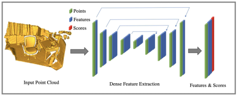
Based on the normalized kernel point convolution, we adopt a UNet-like structure with skip connections and residual blocks to build a fully convolutional network [17], as illustrated in Fig. 1 (Left).
Unlike patch-based methods which only support sparse feature description, our network is able to perform dense feature description under a fully convolutional setting. The output of our network is a dense feature map in the form of a two-dimensional matrix , where is the dimension of the feature vector. The descriptor associated with point is denoted as ,
| (4) |
where denotes the -th row of two-dimensional matrix . The descriptors are L2-normalized to unit length.
3.2 Dense Keypoint Detection
Dusmanu et al. [7] detect keypoints on 2D images based on the local maximum across the spatial and channel dimensions of the feature maps, and use a softmax operator to evaluate the local-max score of a pixel. Due to the regular structure of images, their approach simply selects the neighboring pixels as the neighborhood. To extend their approach to 3D, this strategy might be replaced by radius neighborhood to handle the non-uniform sampling setting of point clouds. However,
the number of neighboring points in the radius neighborhood can vary greatly.
In this case, if we simply use a softmax function to evaluate the local maximum in the spatial dimension, the local regions with few points (e.g., regions close to the boundaries of indoor scenes or far away from Lidar center of outdoor scenes) would inherently have higher scores. To handle this problem, we propose a density-invariant saliency score to evaluate the saliency of a certain point compared with its local neighborhood.
Given the dense feature map , we regard as a collection of 3D response :
| (5) |
where denotes the -th column of the two-dimensional matrix . The criterion of point to be a keypoint is
| (6) | ||||
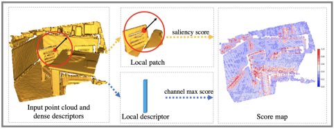
where is the radius neighborhood of . This means that the most preeminent channel is first selected, and then verified by whether or not it is a maximum of its spatial local neighborhood on that particular response map . During training, we soften the above process to make it trainable by applying two scores, as illustrated in Fig. 1 (Right). The details are given below.
Density-invariant saliency score. This score aims to evaluate how salient a point is compared with other points in its local neighborhood. In D2-Net [7], the score evaluating the local-max is defined as
| (7) |
This formulation, however, is not invariant to sparsity. Sparse regions inherently have higher scores than dense areas because the scores are normalized by sum. We therefore design a density-invariant saliency score as follows:
| (8) |
In this formulation, the saliency score of a point is calculated as the difference between its feature and the mean feature of its local neighborhood. Thus it measures the relative saliency of a center point with respect to that of the supporting points in the local region. Besides, using the average response in place of sum (c.f., Equation 7) prevents the score from being affected by the number of the points in the neighborhood. In our experiments (Section 6.4), we will show that our saliency score significantly improves the network’s ability to handle point cloud keypoint detection with varying density.
Channel max score. This score is designed to pick up the most preeminent channel for each point:
| (9) |
Finally, both of the scores are taken into account for the final keypoint detection score:
| (10) |
Thus after we obtain the keypoint score map of an input point cloud, we select points with top scores as keypoints.
4 Joint Optimizating Detection & Description
Designing a proper supervision signal is the key to joint learning of a descriptor and a detector. In this section, We will first describe the metric learning loss for the descriptor, and then design a detector loss from a self-supervised perspective.
Descriptor loss. To optimize the descriptor network, many works attempt to use metric learning strategies, like contrastive loss and triplet loss. We will utilize the contrastive loss, since from our experiments we have found it to give better convergence performance. As for the sampling strategy, we adopt the hardest in batch strategy proposed in [22] to make the network focus on hard pairs.
Given a pair of partially overlapped point cloud fragments and , and a set of pairs of corresponding 3D points. Suppose is a correspondence pair and the two points have their corresponding descriptors and and scores and . The distance between a positive pair is defined as the Euclidean distance between their descriptors as follows:
| (11) |
The distance between a negative pair is,
| (12) |
where is the safe radius, and is the hardest negative sample that lies outside the safe radius of the true correspondences. The contrastive margin loss is defined as
| (13) | ||||
where is the margin for positive pairs and is the margin for negative pairs.
Detector loss. To optimize the detector network, we seek for a loss formulation that encourages the easily matchable correspondences to have higher keypoint detection scores than the correspondences which are hard to match. In [7], Dusmanu et al. proposed an extension to the triplet margin loss to jointly optimize the descriptor and the detector:
| (14) |
where is the triplet margin. They claimed that in order to minimize the loss, the detector network should predict high scores for most discriminative correspondences and vice versa. However, their loss does not provide explicit guidance for the score term, and experimentally we found that their origin loss formulation does not guarantee convergence in our context.
Thus we design a loss term to explicitly guide the gradient of the scores. From a self-supervised perspective, we use the on-the-fly feature matching results to evaluate the discriminativeness of each correspondence, which will guide the gradient flow of the score of each keypoint. If a correspondence is already matchable under the current descriptor network, we want the score to be higher and vice versa. Specifically, we define the detector loss as
| (15) |
Intuitively, if , it indicates that this correspondence can be correctly matched using the nearest neighbor search, and the loss term will encourage the scores and of the two points in the correspondence pair to be higher. Conversely, if , the correspondence is not discriminative enough for the current descriptor network to establish a correspondence, and thus the loss will encourage the scores and to be lower. In order to minimize the loss, the detector should predict higher scores for matchable correspondences and lower scores for non-matchable correspondences.
5 Implementation Details
Training. Our network is implemented in TensorFlow. During training, we use all the point cloud fragment pairs with more than 30% overlap. For each pair of fragments and , we establish the correspondence set by first randomly sampling anchor points from , then applying the ground-truth transformation to these points, and performing nearest neighbor search in fragment . The correspondence is accepted only if the Euclidean distance between two points is less than a threshold. We use grid subsampling to control the number of points and ensure the spatial consistency of point clouds.
For the first layer, we use as our grid size. The neighborhood radius is 2.5 times the grid size of the current layer. The local neighborhood for keypoint detection is the same as the first radius neighborhood. For each point cloud fragment, we apply data augmentation including adding Gaussian noise with standard deviation 0.005, random scaling , and random rotation angle around an arbitrary axis. We use a batch size of 1 and correspondence number . We use positive margin , negative margin for the contrastive loss. The loss terms for the detector and the descriptor are equally weighted. We optimize the network using the Momentum optimizer with an initial learning rate of 0.1, which is exponentially decayed every epoch, and the momentum is set to 0.98. The network converges in about 100 epochs.
Testing. During testing, our keypoint detection module adopts the hard selection strategy formulated by Equation 6 instead of soft selection to get better quality keypoints. This strategy emulates non-maximum suppression and avoids having the selected keypoints lie too close to each other.
6 Experiments
The following sections are organized as follows. First, we demonstrate our method (D3Feat) regarding point cloud registration on 3DMatch dataset [36] (indoor settings) and KITTI [10] dataset (outdoor settings), with the provided data split to train D3Feat. Next, we study the generalization ability of D3Feat on ETH dataset [25] (outdoor settings), using the model trained on 3DMatch dataset. Finally, we more specifically evaluate the keypoint repeatability on 3DMatch and KITTI datasets, to clearly demonstrate the performance of our detector.
6.1 Indoor Settings: 3DMatch dataset
We follow the same protocols in 3DMatch dataset [36] to prepare the training and testing data. In particular, the test set contains scenes with partially overlapped point cloud fragments and their corresponding transformation matrices. For each fragment, randomly sampled 3D points are given for methods that do not include a detector.
Evaluation metrics. Following [2], two evaluation metrics are used including 1) Feature Matching Recall, a.k.a. the percentage of successful alignment whose inlier ratio is above some threshold (i.e., ), which measures the matching quality during pairwise registration. 2) Registration Recall, a.k.a. the percentage of successful alignment whose transformation error is below some threshold (i.e., RMSE m), which better reflects the final performance in practice use. Besides, the intermediate result, Inlier Ratio, is also reported. In above metrics 1) and 3), a match is considered as an inlier if the distance between its corresponding points is smaller than cm under ground-truth transformation. For metric 2), we use a RANSAC with 50,000 max iterations (following [36]) to estimate the transformation matrics.
Comparisons with the state-of-the-arts. We compare D3Feat with the state-of-the-arts on 3DMatch dataset. As shown in Table 1, the Feature Matching Recall is reported regarding two levels of data difficulty: the original point cloud fragments (left columns), and the randomly rotated fragments (right columns). In terms of D3Feat, we report the results both on randomly sampled points (D3Feat(rand)) and on keypoints predicted by our detector network (D3Feat(pred)). In both settings, D3Feat achieves the best performance when a learned detector is equipped.
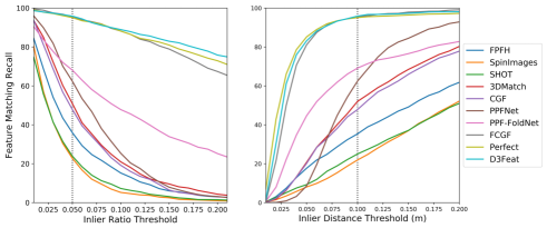
Moreover, we demonstrate the robustness of D3Feat by varying the error threshold (originally defined as cm and ) in Feature Matching Recall. As shown in Fig. 2, we observe that the D3Feat performs consistently well under all conditions. In particular, D3Feat notably outperforms other methods (left figure) under a more strict inlier ratio threshold, e.g., , which indicates the advantage of adopting a detector to derive more distinctive features. In terms of varying , D3Feat performs slightly worse than PerfectMatch [11] when smaller inlier distance error is tolerated, which can be probably ascribed to the small voxel size (1.875cm) used in PerfectMatch, while D3Feat is performed using 3cm voxel downsampling.
| Origin | Rotated | |||
| FMR (%) | STD | FMR (%) | STD | |
| FPFH [28] | 35.9 | 13.4 | 36.4 | 13.6 |
| SHOT [30] | 23.8 | 10.9 | 23.4 | 9.5 |
| 3DMatch [36] | 59.6 | 8.8 | 1.1 | 1.2 |
| CGF [15] | 58.2 | 14.2 | 58.5 | 14.0 |
| PPFNet [5] | 62.3 | 10.8 | 0.3 | 0.5 |
| PPF-FoldNet [4] | 71.8 | 10.5 | 73.1 | 10.4 |
| PerfectMatch [11] | 94.7 | 2.7 | 94.9 | 2.5 |
| FCGF [2] | 95.2 | 2.9 | 95.3 | 3.3 |
| D3Feat(rand) | 95.3 | 2.7 | 95.2 | 3.2 |
| D3Feat(pred) | 95.8 | 2.9 | 95.5 | 3.5 |
Performance under different number of keypoints. To better demonstrate the superiority of a joint learning with a detector, we further report the results when reducing the sampled point number from to 2500, 1000, 500 or even 250. As shown in Table 2, when no detector is equipped, the performance of PerfectMatch, FCGF or D3Feat(rand) drops at a similar magnitude as the number of sampled points get smaller. However, once enabling the proposed detector (D3Feat(pred)), our method is able to maintain a high matching quality regarding all evaluation metrics, and outperform all comparative methods by a large margin.
It is also noteworthy that, regarding Inlier Ratio, D3Feat(pred) is the only method that achieves improved results when smaller number of points is considered. This strongly indicates that the detected keypoints have been properly ranked, and the top points receive higher probability to be matched, which is a desired property that a reliable kepoint is expected to acquire.
| # Keypoints | 5000 | 2500 | 1000 | 500 | 250 |
| Feature Matching Recall (%) | |||||
| PerfectMatch [11] | 94.7 | 94.2 | 92.6 | 90.1 | 82.9 |
| FCGF [2] | 95.2 | 95.5 | 94.6 | 93.0 | 89.9 |
| \hdashlineD2_Triplet | Not Converge | ||||
| D2_Contrastive | 94.7 | 94.2 | 94.0 | 93.2 | 92.3 |
| w/o detector | 95.0 | 94.3 | 94.2 | 92.5 | 90.7 |
| \hdashlineD3Feat(rand) | 95.3 | 95.1 | 94.2 | 93.6 | 90.8 |
| D3Feat(pred) | 95.8 | 95.6 | 94.6 | 94.3 | 93.3 |
| Registration Recall (%) | |||||
| PerfectMatch | 80.3 | 77.5 | 73.4 | 64.8 | 50.9 |
| FCGF | 87.3 | 85.8 | 85.8 | 81.0 | 73.0 |
| D3Feat(rand) | 83.5 | 82.1 | 81.7 | 77.6 | 68.8 |
| D3Feat(pred) | 82.2 | 84.4 | 84.9 | 82.5 | 79.3 |
| Inlier Ratio (%) | |||||
| PerfectMatch | 37.7 | 34.5 | 28.3 | 23.0 | 19.1 |
| FCGF | 56.9 | 54.5 | 49.1 | 43.3 | 34.7 |
| D3Feat(rand) | 40.6 | 38.3 | 33.3 | 28.6 | 23.5 |
| D3Feat(pred) | 40.7 | 40.6 | 42.7 | 44.1 | 45.0 |
Rotation invariance. Previous works such as [5, 11] use sophisticated input representations or per-point local reference frames to acquire rotation invariance. However, as also observed in FCGF [2], we find that a fully convolutional network (e.g., KPConv [33] as used in this paper) is able to empirically achieve strong rotation invariance through low-cost data augmentation, as shown in the right columns of Table 1. We will provide more details about this experiment in supplementary materials.
Ablation study. To study the effect of each component of D3Feat, we conduct thorough ablative experiments on 3DMatch dataset. Specifically, to address the importance of the proposed detector loss, we compare 1) the model trained with the original D2-Net loss (D2_Triplet) and 2) the model trained with the improved D2-Net loss (D2_Contrastive). To demonstrate the benefit from a joint learning of two tasks, we use only the contrastive loss to train a model without the detector learning (w/o detector). Other training or testing settings are kept the same for a fair comparison.
As shown in Table 2, the proposed detector loss (D3Feat(rand)) not only guarantees better convergence than D2_Triplet, but also delivers a notable performance boost over D2_Contrastive. Besides, by comparing w/o detector and D3Feat(rand), it can be seen that a joint learning of a detector is also advantageous to strengthen the descriptor itself.
6.2 Outdoor Settings: KITTI dataset
KITTI odometry dataset comprises 11 image sequences of outdoor driving scenarios for point cloud registration. Following the data splitting method in FCGF [2], we use sequences 0 to 5 for training, 6 to 7 for validation, and 8 to 10 for testing. The ground truth transformations are provided by GPS. To reduce the noise in ground truth, we use the standard iterative closest point (ICP) method to refine the alignment. Besides, only pairs which are at least 10m away from each other are selected. Finally, we train D3Feat with 30cm voxel downsampling for preprocessing.
Evaluation metrics. We evaluate the estimated transformation matrices by two error metrics: Relative Translation Error (RTE) and Relative Rotation Error (RRE) proposed in [8, 21]. The registration is considered accurate if the RTE is below 2m and RRE is below 5∘ following [14].
Comparisions to the state-of-the-arts. We compare D3Feat with FCGF [2] and 3DFeat-Net [14]. For 3DFeat- Net, we report the results as presented in [2]. For FCGF, we use the authors’ implementation trained on KITTI. To compute the transformation, we use RANSAC with 50,000 max iterations. As shown in Table 3, D3Feat outperforms the state-of-the-arts regarding all metrics. Besides, we also show the registration results under different numbers of points in Table 4. In most cases, D3Feat fails to align only one pair of fragments. Even using only 250 points, D3Feat still achieves 99.63% success rate, while FCGF drops to 68.62% due to the lack of a reliable detector.
| RTE(cm) | RRE(∘) | Succ.(%) | |||
| AVG | STD | AVG | STD | ||
| 3DFeat-Net [14] | 25.9 | 26.2 | 0.57 | 0.46 | 95.97 |
| FCGF [2] | 9.52 | 1.30 | 0.30 | 0.28 | 96.57 |
| D3Feat | 6.90 | 0.30 | 0.24 | 0.06 | 99.81 |
| All | 5000 | 2500 | 1000 | 500 | 250 | |
| FCGF [2] | 96.57 | 96.39 | 96.03 | 93.69 | 90.09 | 68.62 |
| D3Feat | 99.81 | 99.81 | 99.81 | 99.81 | 99.81 | 99.63 |
6.3 Outdoor settings: ETH Dataset
In order to evaluate the generalization ability of D3Feat, we use the model trained on 3DMatch dataset and test it on four outdoor laser scan datasets (Gazebo-Summer, Gazebo-Winter, Wood-Summer and Wood-Autumn) from the ETH dataset [25], following the protocols defined in [11]. The evaluation metric is again Feature Matching Recall under the same settings as in previous evaluations. For comparisons, we use the PerfectMatch model with 6.25cm voxel size (16 voxels per 1m), while for FCGF, we use the model trained on 5cm voxel size which we find perform significantly better than the model with 2.5cm on this dataset. For D3Feat, we report the results on both 6.25cm and 5cm to compare with PerfectMatch and FCGF, respectively.
| voxel | Gazebo | Wood | ||||
| size(cm) | Sum. | Wint. | Sum. | Aut. | AVG. | |
| PerfectMatch [11] | 6.25 | 91.3 | 84.1 | 67.8 | 72.8 | 79.0 |
| FCGF [2] | 5.00 | 22.8 | 10.0 | 14.78 | 16.8 | 16.1 |
| D3Feat(rand) | 5.00 | 45.7 | 23.9 | 13.0 | 22.4 | 26.2 |
| D3Feat(pred) | 5.00 | 78.9 | 62.6 | 45.2 | 37.6 | 56.3 |
| D3Feat(pred) | 6.25 | 85.9 | 63.0 | 49.6 | 48.0 | 61.6 |
For a fair comparison, the pre-sampled points provided in [11] are used for PerfectMatch, FCGF and D3Feat(rand) to extract the features. As shown in Table 5, under 5cm voxel size setting, D3Feat demonstrates better generalization ability than FCGF. Once the detector is enabled, the results are improved remarkably. However, on this dataset, PerfectMatch is still the best performing method, whose generalization ability can be mainly ascribed to the use of smoothed density value (SDV) representation, as explained in the original paper [11]. Nevertheless, by comparing the results of D3Feat(rand) and D3Feat(pred), we can still find the significant improvement brought by our detector. The visualization results on ETH can be found in the supplementary materials.
6.4 Keypoint Repeatability
Besides the reliability, a keypoint is also desired to be repeatable. Thus we compare our detector in repeatability with a learning-based method USIP [16] and hand-crafted methods: ISS [37], Harris-3D [13], and SIFT-3D [18] on the 3DMatch test set and KITTI test set.
Evaluation metric. We use the relative repeatability proposed in [16] as the evaluation metric. Specifically, given two partially overlapped point clouds and the ground truth pose, a keypoint in the first point cloud is considered repeatable if its distance to the nearest keypoint in the second point cloud is less than some threshold, under the ground truth transformation. Next, the relative repeatability is calculated as the number of repeatable keypoints over the number of detected keypoints. This threshold is set to 0.1m and 0.5m for 3DMatch and KITTI datasets, respectively.
Implementation. We compare the full model D3Feat, and a baseline model that directly extends the D2-Net design to 3D domain (denoted as D3Feat(base)). We use PCL [27] to implement the classical detectors. For USIP, we take the origin implementation as well as the pretrained model to test on the 3DMatch test set. For the KITTI dataset, since USIP and D3Feat use different processing and splitting strategies and USIP requires surface normal and curvature as input, the results are not directly comparable. Nevertheless, for the sake of completeness, we run and test the original implementation of USIP on our processed KITTI data. For each detector, we generate 4, 8, 16, 32, 64, 128, 256, 512 keypoints and calculate the relative repeatability respectively.
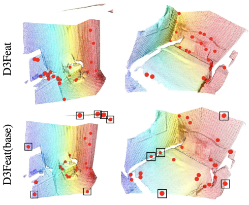
Ablation study. To recap, direct extension from D2-Net to 3D domain brings the problem that points located in more sparse region would have higher probability of being selected as keypoints, which prevents the network from predicting highly repeatable keypoints, as explained in Sec. 3. The proposed density-invariant selection strategy enables the network to handle the inherent density variations of point clouds. In the following, we will demonstrate the effect of proposed keypoint selection strategy through both qualitative and quantitative results.
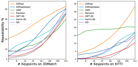
Qualitative results. The relative repeatability in relation to the number of keypoints is shown in Fig. 3. Thanks to the proposed self-supervised detector loss, our detector is encouraged to give higher scores to points with distinctive local geometry while giving lower scores to points with homogeneous neighborhood. Therefore although we do not explicitly supervise the repeatability of keypoints, D3Feat can still achieve comparable repeatability to USIP. D3Feat generally outperforms all the other detectors on 3DMatch and KITTI dataset over all different number of keypoints except worse than USIP on KITTI. In addition, the proposed saliency score significantly improves the repeatability of D3Feat over D3Feat(base), indicating the effectiveness of the proposed keypoint selection strategy.
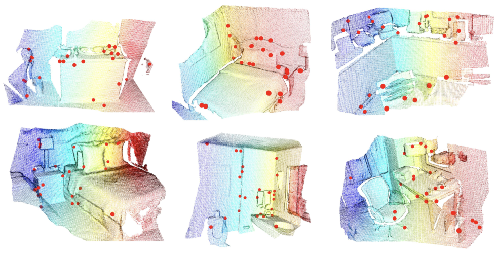
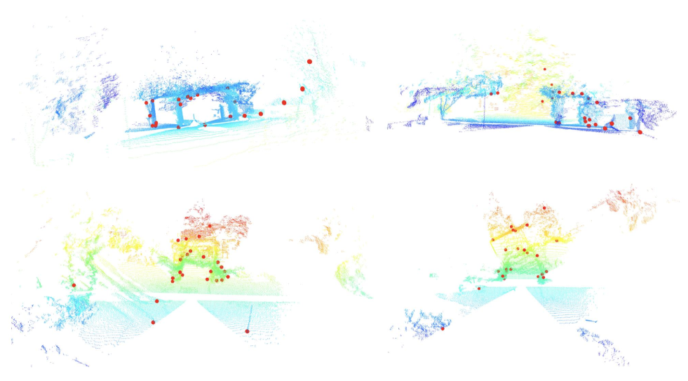
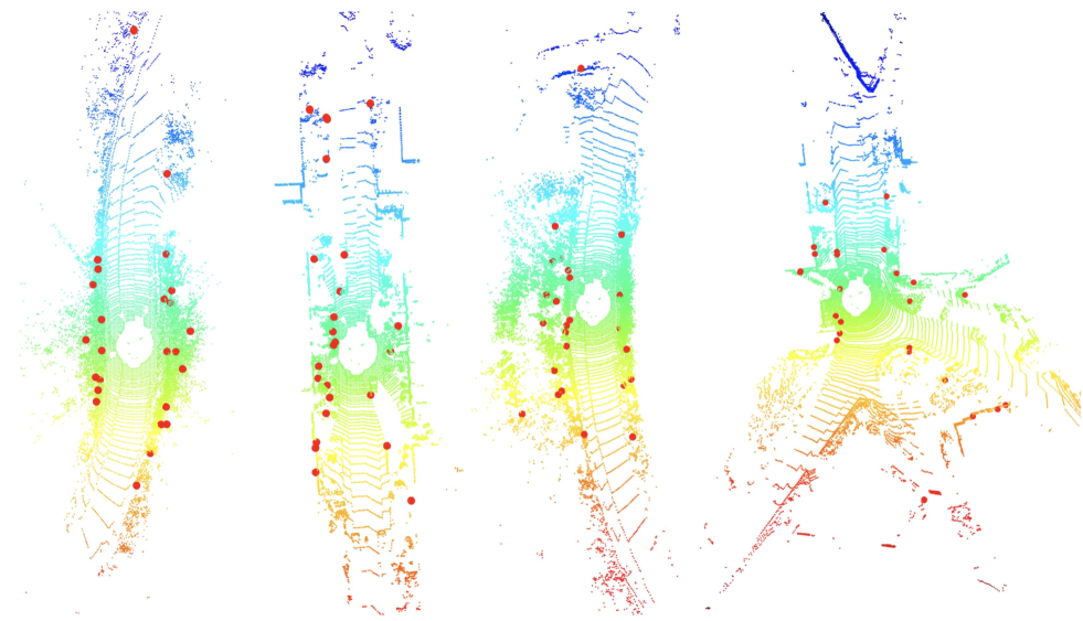
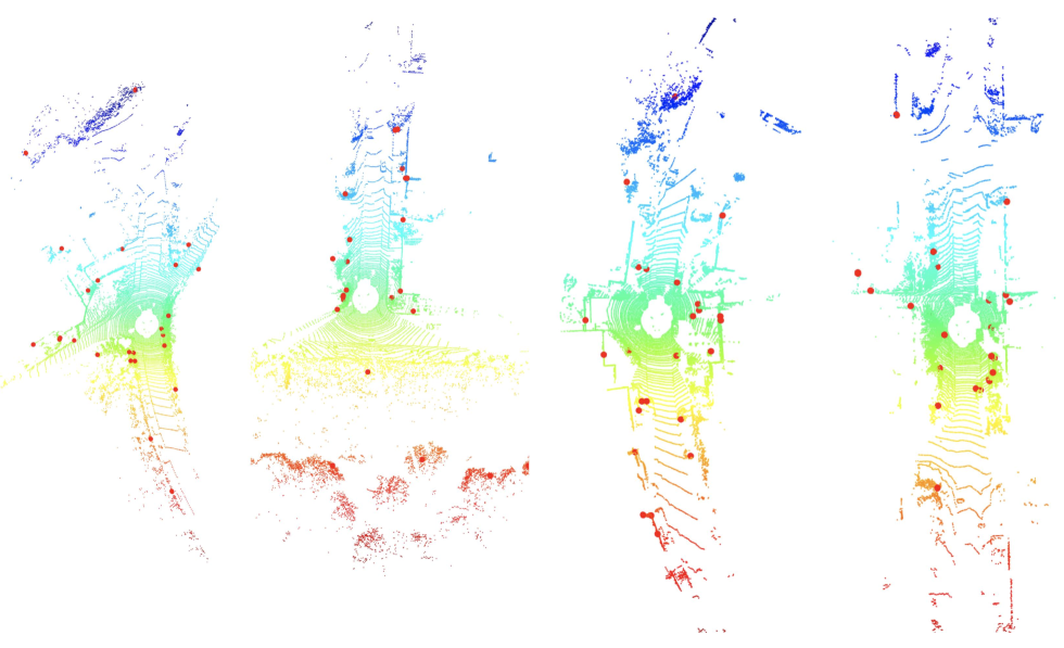
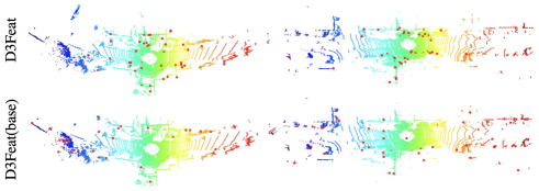
Qualitative results. As shown in Fig. 4 and Fig. 5, the proposed density-invariant selection strategy overcomes the density variations. More qualitative results are included in the supplementary materials.
7 Conclusion
In this paper we have designed a dual-role fully convolutional network for dense feature detection and description on point clouds. A novel density-invariant saliency score has been proposed to help select keypoints under varying densities. Also a self-supervised detector loss has been proposed to guide the network to predict highly repeatable keypoints and enable joint improvement for both detector and descriptor. Extensive experiments on indoor 3DMatch and outdoor KITTI both show the effectiveness of our detector network and the distinctiveness of descriptor network. Our model outperforms the state-of-the-art methods especially when using a small number of keypoints.
Acknowledgement. This work is supported by Hong Kong RGC GRF (No. 16206819 and No. 16203518) and Centre for Applied Computing and Interactive Media (ACIM) of School of Creative Media, City University of Hong Kong.
References
- [1] C. Choy, J. Gwak, and S. Savarese. 4d spatio-temporal convnets: Minkowski convolutional neural networks. In CVPR, 2019.
- [2] C. Choy, J. Park, and V. Koltun. Fully convolutional geometric features. In ICCV, 2019.
- [3] P. H. Christiansen, M. F. Kragh, Y. Brodskiy, and H. Karstoft. Unsuperpoint: End-to-end unsupervised interest point detector and descriptor. arXiv preprint arXiv:1907.04011, 2019.
- [4] H. Deng, T. Birdal, and S. Ilic. Ppf-foldnet: Unsupervised learning of rotation invariant 3d local descriptors. In ECCV, pages 602–618, 2018.
- [5] H. Deng, T. Birdal, and S. Ilic. Ppfnet: Global context aware local features for robust 3d point matching. In CVPR, 2018.
- [6] D. DeTone, T. Malisiewicz, and A. Rabinovich. Superpoint: Self-supervised interest point detection and description. In CVPR Workshops, 2018.
- [7] M. Dusmanu, I. Rocco, T. Pajdla, M. Pollefeys, J. Sivic, A. Torii, and T. Sattler. D2-net: A trainable cnn for joint description and detection of local features. In CVPR, 2019.
- [8] G. Elbaz, T. Avraham, and A. Fischer. 3d point cloud registration for localization using a deep neural network auto-encoder. In CVPR, 2017.
- [9] M. A. Fischler and R. C. Bolles. Random sample consensus: a paradigm for model fitting with applications to image analysis and automated cartography. Communications of The ACM, 1981.
- [10] A. Geiger, P. Lenz, C. Stiller, and R. Urtasun. Vision meets robotics: The kitti dataset. IJRR, 2013.
- [11] Z. Gojcic, C. Zhou, J. D. Wegner, and A. Wieser. The perfect match: 3d point cloud matching with smoothed densities. In CVPR, 2019.
- [12] Y. Guo, M. Bennamoun, F. Sohel, M. Lu, J. Wan, and N. M. Kwok. A comprehensive performance evaluation of 3d local feature descriptors. IJCV, 2016.
- [13] C. G. Harris, M. Stephens, et al. A combined corner and edge detector. In Alvey vision conference, 1988.
- [14] Z. Jian Yew and G. Hee Lee. 3dfeat-net: Weakly supervised local 3d features for point cloud registration. In ECCV, 2018.
- [15] M. Khoury, Q.-Y. Zhou, and V. Koltun. Learning compact geometric features. In ICCV, 2017.
- [16] J. Li and G. H. Lee. Usip: Unsupervised stable interest point detection from 3d point clouds. ICCV, 2019.
- [17] J. Long, E. Shelhamer, and T. Darrell. Fully convolutional networks for semantic segmentation. In CVPR, 2015.
- [18] D. G. Lowe. Distinctive image features from scale-invariant keypoints. IJCV, 2004.
- [19] Z. Luo, T. Shen, L. Zhou, J. Zhang, Y. Yao, S. Li, T. Fang, and L. Quan. Contextdesc: Local descriptor augmentation with cross-modality context. 2019.
- [20] Z. Luo, T. Shen, L. Zhou, S. Zhu, R. Zhang, Y. Yao, T. Fang, and L. Quan. Geodesc: Learning local descriptors by integrating geometry constraints. 2018.
- [21] Y. Ma, Y. Guo, J. Zhao, M. Lu, J. Zhang, and J. Wan. Fast and accurate registration of structured point clouds with small overlaps. In CVPR Workshops, 2016.
- [22] A. Mishchuk, D. Mishkin, F. Radenovic, and J. Matas. Working hard to know your neighbor’s margins: Local descriptor learning loss. In NeurIPS, 2017.
- [23] M. Montemerlo, S. Thrun, D. Koller, B. Wegbreit, et al. Fastslam: A factored solution to the simultaneous localization and mapping problem. Aaai/iaai, 2002.
- [24] Y. Ono, E. Trulls, P. Fua, and K. M. Yi. Lf-net: learning local features from images. In NeurIPS, 2018.
- [25] F. Pomerleau, M. Liu, F. Colas, and R. Siegwart. Challenging data sets for point cloud registration algorithms. IJRR, 2012.
- [26] J. Revaud, P. Weinzaepfel, C. De Souza, N. Pion, G. Csurka, Y. Cabon, and M. Humenberger. R2d2: Repeatable and reliable detector and descriptor. arXiv preprint arXiv:1906.06195, 2019.
- [27] R. Rusu and S. Cousins. 3d is here: Point cloud library (pcl). ICRA, 2011.
- [28] R. B. Rusu, N. Blodow, and M. Beetz. Fast point feature histograms (fpfh) for 3d registration. In ICRA, 2009.
- [29] R. F. Salas-Moreno, R. A. Newcombe, H. Strasdat, P. H. Kelly, and A. J. Davison. Slam++: Simultaneous localisation and mapping at the level of objects. In CVPR, 2013.
- [30] S. Salti, F. Tombari, and L. Di Stefano. Shot: Unique signatures of histograms for surface and texture description. In ECCV, 2010.
- [31] J. L. Schonberger and J.-M. Frahm. Structure-from-motion revisited. In CVPR, 2016.
- [32] H. Su, S. Maji, E. Kalogerakis, and E. Learned-Miller. Multi-view convolutional neural networks for 3d shape recognition. In ICCV, 2015.
- [33] H. Thomas, C. R. Qi, J.-E. Deschaud, B. Marcotegui, F. Goulette, and L. J. Guibas. Kpconv: Flexible and deformable convolution for point clouds. ICCV, 2019.
- [34] F. Tombari, S. Salti, and L. Di Stefano. Performance evaluation of 3d keypoint detectors. IJCV, 2013.
- [35] K. M. Yi, E. Trulls, V. Lepetit, and P. Fua. Lift: Learned invariant feature transform. In ECCV, 2016.
- [36] A. Zeng, S. Song, M. Nießner, M. Fisher, J. Xiao, and T. Funkhouser. 3dmatch: Learning local geometric descriptors from rgb-d reconstructions. In CVPR, 2017.
- [37] Y. Zhong. Intrinsic shape signatures: A shape descriptor for 3d object recognition. In ICCV Workshops, 2009.
- [38] L. Zhou, S. Zhu, Z. Luo, T. Shen, R. Zhang, M. Zhen, T. Fang, and L. Quan. Learning and matching multi-view descriptors for registration of point clouds. In ECCV, 2018.
- [39] Q.-Y. Zhou, J. Park, and V. Koltun. Open3d: A modern library for 3d data processing. arXiv preprint arXiv:1801.09847, 2018.
8 Supplementary Material
In this supplementary material, we first explain the details about our modification on KPConv [33], then we analyze the contribution of rotation augmentation by an ablation study on 3DRotatedMatch dataset. We further conduct the ablative experiments on the detector loss as well as incorporating our detector with FCGF. Finally, we provide additional details about the experiments on 3DMatch, KITTI and ETH datasets and some further visualization results.
8.1 Implementation Details
Normalization term As explained in the main paper, the original formulation of KPConv is not invariant to point density. Thus we add a density normalization term, which sums up the number of the supporting points in the neighborhood, to ensure that the convolution is sparsity invariant. To demonstrate the effectiveness of the normalization term, we train networks with and without the normalization term in the same settings with what is described in the main paper, and report the registration results on 3DMatch dataset. During testing, instead of using voxel downsample, we use uniform downsample i.e. uniform_down_sample in Open3D [39] implementation, by which the density variations of input point clouds is enlarged. We evaluate the model on sample rate , which leads to a similar average number of points for the point clouds in the test set. The result is shown in Table 6.
| Voxel | Uniform | |||||
| 5000 | 5000 | 2500 | 1000 | 500 | 250 | |
| w/o norm. | 95.6 | 77.3 | 76.5 | 73.9 | 71.4 | 66.1 |
| w norm. | 95.8 | 91.9 | 91.8 | 91.2 | 90.2 | 89.4 |
As shown in Table 6, the normalization term is effective to handle neighborhoods with different sparsity levels. When using a uniform downsample strategy, D3Feat with the normalization term is able to maintain a high matching quality, and outperform the model without the normalization term by a large margin.
Network architecture We adopt the architecture for segmentation tasks proposed in KPConv [33]. The number of channels in the encoder part are . Skip connections are used between the corresponding layers of the encoder part and the decoder part. The output features are processed by a 11 convolution to get the final 32 dimensional features. Other settings are the same with original paper [33].
8.2 Ablation on Rotation Invariance
In experiments, we find that a fully convolutional network is able to empirically achieve strong rotation invariance through low cost data augmentation. To demonstrate the effectiveness of simple data augmentation on the robustness to rotation, we further train the model without rotation augmentation and evaluate it on 3DRotatedMatch dataset. The result is shown in Table 7.
| 5000 | 2500 | 1000 | 500 | 250 | |
| w/o aug. | 5.5 | 5.4 | 4.9 | 5.4 | 5.5 |
| w aug. | 95.5 | 95.0 | 94.8 | 92.1 | 88.9 |
Without rotation augmentation, D3Feat fails on 3DRotatedMatch because the network cannot learn the rotation invariance from the data.
8.3 Ablation on Detector Loss
To better analyze the contribution of the proposed detector loss, we re-create a table below, which derives original results from Table 2, and the results from our model without the detector loss and performing on the predicted keypoints(w/o detector (pred)). The effect of detector loss can be seen from the comparison between w/o detector and D3Feat on both random (rand) or predicted (pred) points. It is shown that the detector loss not only strengthens the descriptor itself (given random keypoints), but also boosts the performance of the detector (given predicted keypoints). It is also noteworthy that only D3Feat(pred) improves the Inlier Ratio when reducing the number of points, which clearly indicates that the detector loss helps to better rank the keypoints regarding distinctiveness.
| # Keypoints | 5000 | 2500 | 1000 | 500 | 250 |
| Feature Matching Recall (%) | |||||
| w/o detector(rand) | 95.0 | 94.3 | 94.2 | 92.5 | 90.7 |
| w/o detector(pred) | 95.2 | 95.0 | 94.5 | 92.4 | 90.4 |
| \hdashlineD3Feat(rand) | 95.3 | 95.1 | 94.2 | 93.6 | 90.8 |
| D3Feat(pred) | 95.8 | 95.6 | 94.6 | 94.3 | 93.3 |
| Inlier Ratio (%) | |||||
| w/o detector(rand) | 40.7 | 39.9 | 35.2 | 31.0 | 25.1 |
| w/o detector(pred) | 41.7 | 40.3 | 38.7 | 36.6 | 33.2 |
| \hdashlineD3Feat(rand) | 40.6 | 38.3 | 33.3 | 28.6 | 23.5 |
| D3Feat(pred) | 40.7 | 40.6 | 42.7 | 44.1 | 45.0 |
8.4 Ablation on Detector with FCGF
Since the detection scores are computed on top of the extracted dense descriptors, it is easy to incorporate our detector with other dense feature description models, such as FCGF [2]. To demonstrate the usability of our method, we train the FCGF with the proposed joint learning method and evaluate it on the 3DMatch dataset, as shown in Table 9. The model FCGF + detector is trained using the proposed detector loss under the same setting with [2] for 100 epochs.
| # Keypoints | 5000 | 2500 | 1000 | 500 | 250 |
| Registration Recall (%) | |||||
| FCGF[2] | 87.3 | 85.8 | 85.8 | 81.0 | 73.0 |
| FCGF + detector | 86.7 | 87.8 | 88.3 | 85.4 | 81.5 |
| Inlier Ratio (%) | |||||
| FCGF[2] | 56.9 | 54.5 | 49.1 | 43.3 | 34.7 |
| FCGF + detector | 53.5 | 53.2 | 53.6 | 53.2 | 51.0 |
The result shows that FCGF can indeed benefit from the proposed joint learning and maintain a high performance given a smaller number of points.
8.5 Runtime
To demonstrate the efficiency of our method, we compare the runtime of D3Feat with FCGF [2] on 3DMatch in Table 10. For a fair comparison, we use the same voxel size (2.5cm, roughly 20k points) with FCGF to measure the runtime of D3Feat including both detection and description. The performance difference mainly lies in the sparse convolution used by FCGF, which is time-consuming in hashing.
| CPU | GPU | Time(s) | |
| FCGF[2] | Intel 10-core 3.0GHz(i7-6950) | Titan-X | 0.36 |
| D3Feat | Intel 4-core 4.0GHz(i7-4790K) | GTX1080 | 0.13 |
8.6 Evaluation Metric for 3DMatch
Feature matching recall Feature matching recall is first proposed in [5], which measures the quality of features without using a RANSAC pipeline. Given two partially overlapped point cloud and , and the descriptor network denoted as a non-linear function mapping from input points to feature descriptors, the correspondence set for the fragments pairs is obtained by mutually nearest neighbor search in feature space,
| (16) | ||||
where denotes the nearest neighbor search based on the Euclidean distance. Finally the feature matching recall is defined as,
| (17) |
where is the set of point cloud fragment pairs which have more than 30% overlap, and is the ground truth transformation between the fragment pair . is the inlier distance threshold between a correspondence pair, and is the inlier ratio threshold of the fragment pair. Following the setting of [36], the correspondence which have less than euclidean distance between their descriptors are seen as inliers, and the fragment pairs which have more than inlier correspondences will be counted as one match. The evaluation metric is based on the theoretical analysis that RANSAC need iterations to achieve 99.9% confidence of finding at least 3 correspondence with inlier ratio 5%.
Registration recall Registration recall [36] measures the quality of features within a reconstruction system, which firstly uses a robust local registration algorithm like RANSAC to estimate the rigid transformation between two point clouds, then calculate the RMSE of the ground truth correspondence under the estimated transformation. The ground truth correspondence set for fragments pair and is given,
| (18) |
then the registration recall is defined as,
| (19) |
where is the transformation matrix estimated by RANSAC. In our experiment, we run a maximum of 50,000 iterations on the initial correspondence set to estimate the transformation between fragments following [36].
8.7 Dataset Preprocessing
This section provides the steps to process the datasets including 3DMatch, 3DRotatedMatch, KITTI and ETH.
3DMatch For training set, we follow the steps in [36] to get fused point cloud fragments and corresponding poses. We find all the fragments pairs that have more than overlap to build the training set. During training, we alternate between selecting the nearby fragment as the corresponding pair, or randomly selecting from all the overlapped fragments for fast convergence. For test set, we directly use the point cloud fragments and ground truth poses provided by the authors without performing any preprocess to extract the dense feature and score map.
3DRotatedMatch Our model is inherently translation invariant because we are using the relative coordinates. So in order to test the robustness of our model to rotation, we create the 3DRotatedMatch test set following [4]. We rotate all the fragments in 3DMatch test set along all three axes with random sampled angle from a uniform distribution over [0, 2).
KITTI The training set of KITTI odometry dataset contains 11 sequences, we use sequence 0 to 5 for training, sequence 6 to 7 for validation and the last three for testing. Since GPS ground truth is noisy, we first use ICP to refine the alignment and then verify by whether enough correspondence pairs can be found. We select Lidar scan pairs with at least 10m intervals to obtain 1358 pairs for training, 180 pairs for validation and 555 for testing.
ETH For a fair comparison, we directly use the raw point clouds, the ground-truth transformations along with the overlap ratio provided by the authors of [11] to extract the features and evaluate the registration results.
8.8 Qualitative Visualization
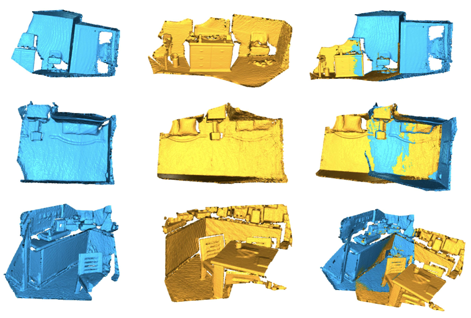
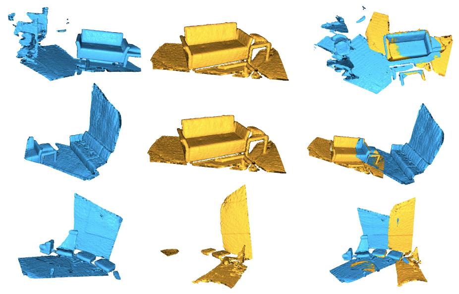
We show some challenging registration results in Figure 6 and more visualizations of detected keypoints on 3DMatch, ETH, KITTI in Figure 7, 8, 9, respectively.
