On the equivalence of the Hermitian eigenvalue problem and hypergraph edge elimination

Abstract

It is customary to identify sparse matrices with the corresponding adjacency or incidence graph. For the solution of linear systems of equations using Gaussian elimination, the representation by its adjacency graph allows a symbolic computation that can be used to predict memory footprints and enables the determination of near-optimal elimination orderings based on heuristics. The Hermitian eigenvalue problem on the other hand seems to evade such treatment at first glance due to its inherent iterative nature. In this paper we prove this assertion wrong by showing the equivalence of the Hermitian eigenvalue problem with a symbolic edge elimination procedure. A symbolic calculation based on the incidence graph of the matrix can be used in analogy to the symbolic phase of Gaussian elimination to develop heuristics which reduce memory footprint and computations. Yet, we also show that the question of an optimal elimination strategy remains NP-hard, in analogy to the linear systems case.

1 Introduction

The divide-and-conquer algorithm is a well-known method for computing the eigensystem (eigenvalues and, optionally, associated eigenvectors) of a Hermitian tridiagonal matrix [4, 6, 7]. It can be parallelized efficiently [2, 7], and even serially it is among the fastest algorithms available [1, 6].

The method relies on the fact that if the eigensystem of a Hermitian matrix $A_{0}$ is known, then the eigenvalues of a “rank-$1$ modification” (or “rank-$1$ perturbation”) of this matrix, $A_{1}=A_{0}+\rho zz^{H}$, can be determined efficiently by solving the so-called “secular equation” [3, 10], and $A_{1}$’s eigenvectors can also be obtained from those of $A_{0}$ [11].

In the tridiagonal case this can be used to zero out a pair of off-diagonal entries $t_{k+1,k}$ and $t_{k,k+1}=\overline{t_{k+1,k}}$ near the middle of the tridiagonal matrix $T$ such that $T$ decomposes into two half-size matrices and a rank-$1$ modification,

$$T=\left[\begin{array}[]{@{}cc@{}}T_{1}&0\\ 0&T_{2}\end{array}\right]\pm t_{k+1,k}zz^{H},$$

with a vector $z$ containing nonzeros at positions $k$ and $k+1$ and zeros elsewhere. Having computed the eigensystems of $T_{1}$ and $T_{2}$ (by recursive application of the same scheme), the eigensystem of $T$ is obtained from these using the rank-$1$ machinery.

In this work we extend this method to a more general setting. In Section 2 we show that the eigensystem of a Hermitian matrix can be computed via a sequence of rank-$1$ modifications, each of them removing entries of the matrix until a diagonal matrix is reached. Section 3 reviews some of the theory for rank-$1$ modifications, as far as this is essential for the following discussion.

While this approach in principle also works for full matrices, it benefits heavily from sparsity. In Section 4 we show that the necessary work for a whole sequence of rank-$1$ modifications can be modelled in a graph setting, similarly to the fill-in arising in direct solvers for Hermitian positive definite linear systems; cf., e.g., [5, 9]. However, the removal of nodes from the graph associated with the matrix is not sufficient to fully describe the progress of the eigensolver; here, the removal of edges in hypergraphs [14] provides a natural description.

We present two ways to come back to node elimination. In Section 5 we consider the dual hypergraph, and in Section 6 we will see that the edge elimination is closely related to Gaussian elimination for the so-called edge–edge adjacency matrix (and thus to node elimination on the graph associated with that matrix). In particular, an NP-completeness result will be derived from this relation in Section 7. This result implies that, for a given sequence of rank-$1$ modifications, it will not be practical to determine an ordering of this sequence that is optimal in a certain sense.

Nevertheless, the hypergraph-based models allow to devise heuristics for choosing among possible sequences of rank-$1$ modifications such that the overall consumption of resources is reduced. In Section 8 we discuss heuristics for the elimination orderings to reduce memory footprint and computations.

Throughout the paper we assume that $A\in\mathbb{C}^{n\times n}$ is Hermitian. The presentation is aimed at sparse matrices, but “sparsity” is to be understood in the widest sense, including full matrices.

2 Successive edge elimination

We first show that the Hermitian eigenvalue problem $AQ=Q\Lambda$ can be solved by a series of rank-$1$-modified eigenvalue problems. One way to do this is to have each rank-$1$ modification remove one pair of nonzero off-diagonal entries $a_{k,\ell}$ and $a_{\ell,k}=\overline{a_{k,\ell}}$, which in turn correspond to a pair of edges of the graph associated to $A$. Thus we first introduce the basic graph notation we require.

Definition 2.1.

The directed adjacency graph $G_{A}=(V,E)$ with vertex set $V$ and edge set $E$ that is associated with $A\in\mathbb{C}^{n\times n}$ is defined by

$$V=\{1,\ldots,n\}\quad\text{and}\quad E=\{(k,\ell)\in V^{2}\mid k\not=\ell,\ a_{k,\ell}\neq 0\}.$$

As our method treats matrix entries by conjugate pairs and maintains Hermiticity throughout, it is sufficient to consider only the lower triangle of the matrix, corresponding to $E^{\,\includegraphics[width=3.61664pt]{ltriang}}=\{e=(k,\ell)\in E\mid k>\ell\}$.

Definition 2.2.

For each edge $(k,\ell)\in E^{\,\includegraphics[width=3.61664pt]{ltriang}}$ with $a_{k,\ell}=r_{k,\ell}\cdot e^{i\theta_{k,\ell}}\in\mathbb{C}$, where $r_{k,\ell}=|a_{k,\ell}|$, we define a vector representation $z_{(k,\ell)}\in\mathbb{C}^{n}$ of the edge by

$$\left(z_{(k,\ell)}\right)_{j}=\begin{cases}1&\text{if\ }j=\ell,\\ e^{i\theta_{k,\ell}}&\text{if\ }j=k,\\ 0&\text{else}.\end{cases}$$

Using these vectors we can rewrite $A$ as a sum of rank-$1$ modifications to a diagonal matrix.

Lemma 2.3.

Let $A\in\mathbb{C}^{n\times n}$ be sparse and Hermitian with associated graph $G_{A}=(V,E)$. Then

$$A=D+\sum_{(k,\ell)\in E^{\,\includegraphics[width=2.58331pt]{ltriang}}}r_{k,\ell}\cdot z_{(k,\ell)}z_{(k,\ell)}^{H},$$ (1)

where $D=\operatorname{diag}(d_{1},\ldots,d_{n})$ with

$$d_{i}\ =\ a_{i,i}-\sum_{(k,\ell)\in E^{\,\includegraphics[width=2.58331pt]{ltriang}},k=i\;\mathrm{or}\;\ell=i}r_{k,\ell}\ =\ a_{i,i}-\sum_{j=1,j\not=i}^{n}|a_{i,j}|.$$ (2)

Proof.

For each edge $(k,\ell)$ with $k>\ell$, the rank-$1$ matrix $r_{k\ell}\cdot z_{(k,\ell)}z_{(k,\ell)}^{H}$ is nonzero only at the four positions $\{\ell,k\}\times\{\ell,k\}$, where we find

$$\Big{(}r_{k,\ell}\cdot z_{(k,\ell)}z_{(k,\ell)}^{H}\Big{)}_{\{\ell,k\}\times\{\ell,k\}}=r_{k,\ell}\begin{bmatrix}1&e^{-i\theta_{k,\ell}}\\ e^{i\theta_{k,\ell}}&1\end{bmatrix}=\begin{bmatrix}r_{k,\ell}&\overline{a_{k,\ell}}\\ a_{k,\ell}&r_{k,\ell}\end{bmatrix}.$$

Thus the $i$th diagonal entry is changed only by those edges starting or ending at node $i$, which gives the first equality in eq. 2. The second equality is a direct consequence of the definition of $E^{\,\includegraphics[width=3.61664pt]{ltriang}}$ and the Hermiticity of $A$. ∎

Remark 2.4.

The entries of $D$ in eq. 1 correspond to the lower bounds of the Gershgorin intervals. By defining $z_{(k,\ell)}$ differently one can also obtain a representation of $A$ similar to eq. 1 such that the entries of $D$ correspond to the upper bounds of the Gershgorin intervals.

The solution of the Hermitian eigenvalue problem starting from eq. 1 is now straight-forward. Fixing an ordering of the edges, i.e., defining $E^{\,\includegraphics[width=3.61664pt]{ltriang}}=\{e_{1},\ldots,e_{|E^{\,\includegraphics[width=2.58331pt]{ltriang}}|}\}$ we have

$$A=\left(D+r_{e_{1}}\cdot z_{e_{1}}z_{e_{1}}^{H}\right)+\sum_{j=2}^{|E^{\,\includegraphics[width=2.58331pt]{ltriang}}|}r_{e_{j}}\cdot z_{e_{j}}z_{e_{j}}^{H}.$$ (3)

Assuming that the eigendecomposition of the Hermitian matrix $D+r_{e_{1}}\cdot z_{e_{1}}z_{e_{1}}^{H}$ has been computed,

$$D+r_{e_{1}}\cdot z_{e_{1}}z_{e_{1}}^{H}=Q_{1}D_{1}Q_{1}^{H}$$

with $Q_{1}$ unitary, we can rewrite eq. 3 as

$$A=Q_{1}\Bigg{(}D_{1}+\sum_{j=2}^{|E^{\,\includegraphics[width=2.58331pt]{ltriang}}|}r_{e_{j}}\cdot\left(Q_{1}^{H}z_{e_{j}}\right)\left(Q_{1}^{H}z_{e_{j}}\right)^{H}\Bigg{)}Q_{1}^{H},$$

i.e., we eliminated edge $e_{1}$ from eq. 1. Successive elimination of the remaining $|E^{\,\includegraphics[width=3.61664pt]{ltriang}}|-1$ edges, involving the vector $Q_{j-1}^{H}\cdots Q_{1}^{H}\cdot z_{e_{j}}=(\prod_{i=1}^{j-1}Q_{i})^{H}\cdot z_{e_{j}}$ in step $j$, finally yields the eigendecomposition of $A$,

$$A=\Bigg{(}\prod_{j=1}^{|E^{\,\includegraphics[width=2.58331pt]{ltriang}}|}Q_{j}\Bigg{)}\,D_{|E^{\,\includegraphics[width=2.58331pt]{ltriang}}|}\,\Bigg{(}\prod_{j=1}^{|E^{\,\includegraphics[width=2.58331pt]{ltriang}}|}Q_{j}\Bigg{)}^{H}.$$

This approach is summarized in Algorithm 2.1.

1 Write $A=D_{0}+\sum_{e\in E^{\,\includegraphics[width=2.58331pt]{ltriang}}}r_{e}\cdot z_{e}z_{e}^{H}$

2 Choose an ordering of the edges $e_{1},e_{2},\ldots,e_{|E^{\,\includegraphics[width=2.58331pt]{ltriang}}|}$

3 Set $Q=I$

4 for $j=1$ to $|E^{\,\includegraphics[width=3.61664pt]{ltriang}}|$ 

5       Calculate eigendecomposition of $D_{j-1}+r_{e_{j}}\cdot z_{e_{j}}z_{e_{j}}^{H}=Q_{j}D_{j}Q_{j}^{H}$

6       for $i=j+1$ to $|E^{\,\includegraphics[width=3.61664pt]{ltriang}}|$ 

7             $z_{e_{i}}=Q_{j}^{H}\cdot z_{e_{i}}$

8            

9      $Q=QQ_{j}$

10      

Algorithm 2.1 Successive edge elimination.

In order to be able to compute the eigendecomposition in this way we need an efficient way to solve eigenproblems of the kind “diagonal plus rank-$1$ matrix.” It is well known that these problems can be easily dealt with in terms of the secular function, as we review in Section 3. In order to come up with a symbolic representation of the elimination procedure we have to analyze the effect of the elimination of a particular edge $e_{j}$ on the remaining edges. This symbolic representation is developed in Section 4.

3 Computing eigenvalues of rank-$1$-modified matrices

In order to clarify the main tool needed throughout the remainder of this work we review some classical results about the eigenvalues of rank-$1$ perturbed matrices. The results cited here date back to [8] and are also contained in [12, pp. 94–98]. They were later-on used in [3, 4] to formulate the divide-and-conquer method for tridiagonal eigenproblems.

Theorem 3.1 ([3, Theorem 1]).

Let $D+\rho zz^{H}=Q\Lambda Q^{H}$ be the eigendecomposition of the rank-$1$-modified matrix, where $D=\operatorname{diag}(d_{1},\ldots,d_{n})\in\mathbb{R}^{n\times n}$ with $d_{1}\leq d_{2}\leq\ldots\leq d_{n}$, $\|{z}\|=1$, and $\rho>0$. Then the diagonal entries of $\Lambda=\operatorname{diag}(\lambda_{1},\ldots,\lambda_{n})$ are the roots of the “secular equation”

$$f(\lambda)=1+\rho\sum_{j=1}^{n}\frac{|z_{j}|^{2}}{d_{j}-\lambda}.$$ (4)

More specifically, let the $\lambda_{j}$ be ordered, $\lambda_{1}\leq\lambda_{2}\leq\ldots\leq\lambda_{n}$. Then it holds

$$\lambda_{j}=d_{j}+\rho\mu_{j}\quad\text{with}\quad 0\leq\mu_{j}\leq 1\text{\ for\ }j=1,\ldots,n\quad\text{and}\quad\sum_{j=1}^{n}\mu_{j}=1.$$ (5)

There are two important consequences of Theorem 3.1 found in [12, pp. 94–98].

Lemma 3.2.

Using the same notation as in Theorem 3.1 we obtain the following.

1. In case the eigenvalues of $D$ are pairwise different we find that $\lambda_{j}=d_{j}$ if and only if $z_{j}=0$.

2. In addition, if all $z_{j}\neq 0$, we find that $d_{j}<\lambda_{j}<d_{j+1},j=1,\ldots,n$ ($d_{n+1}=\infty$).

3. Assume there exists a multiple eigenvalue $d_{j}$ of $D$ with multiplicity $k$; w.l.o.g. $d_{j-k+1}=\ldots=d_{j-1}=d_{j}$ and $\|{z_{j-k+1,\ldots,j}}\|\neq 0$. Then we find

   $$\lambda_{i}=d_{i},\ i=j-k+1,\ldots,j-1,\quad\text{and}\quad d_{j}<\lambda_{j}<d_{j+1}\quad(d_{n+1}=\infty).$$

Lemma 3.2 is one of the key algorithmic ingredients of the divide-and-conquer algorithm for tridiagonal eigenproblems and known in this context as “deflation.”

As described in [7] and exploited in the implementation of the divide-and-conquer method, the root-finding problem of eq. 4 is highly parallel and can be efficiently solved by a modified Newton iteration using hyperbolae instead of linear ansatz functions.

Recall that in our context the vector for the $j$th rank-$1$ modification (elimination of $e_{j}$) is $(\prod_{i=1}^{j-1}Q_{i})^{H}\cdot z_{e_{j}}$. Therefore, Lemma 3.2 implies that this elimination only requires the solution of the secular equation in at most

$$N_{e_{j}}=\operatorname{nnz}\Big{(}(\prod_{i<j}Q_{i})^{H}\cdot z_{e_{j}}\Big{)}$$ (6)

intervals, where $\operatorname{nnz}(v)$ is the number of nonzero entries of a vector $v$. That is, at most $N_{e_{j}}$ of the entries of $D_{j-1}$ (i.e., eigenvalue approximations) change from $D_{j-1}$ to $D_{j}$. Further, by Theorem 3.1 we obtain that all eigenvalues move in the same direction and the total displacement of these eigenvalues is given by $r_{e_{j}}\cdot\|(\prod_{i<j}Q_{i})^{H}\cdot z_{e_{j}}\|^{2}=2|a_{e_{j}}|$ because $r_{e_{j}}=|a_{e_{j}}|$ and the norm of the vector, $\|z_{e_{j}}\|=\sqrt{2}$, does not change under the orthogonal transformation $(\prod_{i<j}Q_{i})^{H}$.

Using the above reasoning, one would be able to estimate the cost of the overall elimination process for a given ordering of the edges, if the number of nonzeros in the vectors $(\prod_{i<j}Q_{i})^{H}z_{e_{j}}$ could be predicted. In the following section we show how to do this.

Being able to analyze the influence of the ordering of the edges on the complexity of the calculations (in terms of the number of roots of the secular equations that need to be calculated) also allows us to determine an ordering that leads to low overall cost. This topic is discussed in Sections 7 and 8.

4 Edge elimination, hypergraphs and edge elimination in hypergraphs

In Section 2 we have seen that the eigendecomposition of a Hermitian (sparse) matrix $A$ can be obtained by successively eliminating the edges $e_{1},e_{2},\ldots,e_{|E^{\,\includegraphics[width=2.58331pt]{ltriang}}|}$ of the graph $G_{A}$ associated with the matrix $A$.

It is well known that in the context of Gaussian elimination for Hermitian positive definite matrices, the effect of eliminating one node (corresponding to selecting a pivot row and doing the row additions with this row) directly shows in the (undirected) graph $G_{A}$: removing the node and connecting all its former neighbors introduces exactly those edges that correspond to the new fill-in produced by the row operations [5, 9]. This allows to determine the nonzero patterns of the matrix during the whole Gaussian elimination before doing any floating-point operation.

A similar thing can be done for the nonzero patterns of the vectors $(\prod_{i<j}Q_{i})^{H}z_{e_{j}}$ resulting from preceding eliminations. However, as we are eliminating edges, the graph $G_{A}$ is not adequate for this purpose. We have to generalize the concept of a graph and use what is known in the literature as a hypergraph [14].

Definition 4.1.

An undirected hypergraph $G=(V,E)$ is defined by a set of vertices $V=\{v_{1},\ldots,v_{n}\}$ and a set of hyperedges $E=\{e_{1},\ldots,e_{m}\}$, where $\emptyset\not=e_{j}\subseteq V$.

Example 4.2.

The hypergraph with vertex set $V=\{1,2,3,4,5\}$ and set of hyperedges $E=\{e_{1},e_{2},e_{3},e_{4}\}=\left\{\{1,2,5\},\{2,3\},\{1,3,4,5\},\{3,4\}\right\}$ is depicted in Figure 1, where each edge in represented by a closed line that contains all its vertices.

Figure 1: Drawing of the hypergraph defined in Example 4.2 with $V=\{1,2,3,4,5\}$ and hyperedges $e_{1}=\{1,2,5\},e_{2}=\{2,3\},e_{3}=\{1,3,4,5\}$ and $e_{4}=\{3,4\}$.

Remark 4.3.

The possibility to have edges with more or less vertices than two is the only difference to the usual definition of an undirected graph. In particular, the graph $G_{A}$ can be considered as a hypergraph if we include each pair of edges $(k,\ell)$, $(\ell,k)$ only once, i.e., if we replace $E$ with $E^{\,\includegraphics[width=3.61664pt]{ltriang}}$.

In order to analyze the nonzero pattern of the vector $(\prod_{i<j}Q_{i})^{H}z_{e_{j}}$ for the $j$th rank-$1$ modification we first note that this vector can be obtained in two ways: “left-looking,” when it is needed, by accumulating all previous transformations $Q_{i}^{H}$ ($i<j$), or “right-looking,” by applying each transformation $Q_{i}^{H}$, once it has been computed, to all later $z_{j}$. In the following discussion, as well as in Algorithm 2.1, the right-looking approach is taken.

We now consider the effect of one such operation from the matrix/vector point of view. Let us assume that the edges are ordered and focus on the elimination of the first edge, $e_{1}$. Assume w.l.o.g. that $e_{1}=\{1,2\}$. By definition, $z_{e_{1}}$ has only two nonzero entries at the indices $1$ and $2$, and thus due to Theorem 3.1 and Lemma 3.2 we find

$$Q_{1}=\left[\begin{matrix}q_{11}&q_{12}&\\ q_{21}&q_{22}&\\ &&I_{(n-2)\times(n-2)}\end{matrix}\right].$$

Hence, for all edges $e_{j}$ with $e_{j}\cap e_{1}=\emptyset$ we have $Q_{1}^{H}\cdot z_{e_{j}}=z_{e_{j}}$. On the other hand, for all edges $e_{j}$ with $e_{j}\cap e_{1}\neq\emptyset$ we find that $Q_{1}^{H}\cdot z_{e_{j}}$ has entries at the indices $e_{j}\cup e_{1}$.

The situation for the $i$th elimination step is similar. Let the hyperedge $e_{j}$ denote the nonzero pattern, i.e., the set of the positions of the nonzeros, of the current vector $z_{j}$ (after the preceding transformations $Q_{i-1}^{H}\cdots Q_{1}^{H}\cdot z_{j}$). Then the transformed vector $Q_{i}^{H}\cdot z_{j}$ will have nonzeros at the same positions $e_{j}$ if $e_{j}\cap e_{i}=\emptyset$ and at positions $e_{j}\cup e_{i}$ if the two hyperedges overlap.

Remark 4.4.

Strictly speaking this holds only if the transformation $Q_{i}^{H}\cdot z_{j}$ does not introduce new (“cancellation”) zeros in the vector. In the symbolic processing for sparse linear systems it is commonly assumed that this does not happen; we will do so as well.

We summarize the above observation in the following theorem.

Theorem 4.5.

Let $G=(V,E)$ be an undirected hypergraph with $E\neq\emptyset$. Let $x\in E$ be the edge to be eliminated, and let

$$E=E_{x}\cup E_{\not x},\quad\text{where}\quad\begin{cases}E_{x}=\{e\in E\mid e\cap x\neq\emptyset\}\text{\ and}\\ E_{\not x}=\{e\in E\mid e\cap x=\emptyset\}.\end{cases}$$

Then the hypergraph after elimination of $x$ is given by $\widetilde{G}=(\widetilde{V},\widetilde{E})$ with $\widetilde{V}=V$ and $\widetilde{E}=\{e\cup x,e\in E_{x}\setminus\{x\}\}\cup E_{\not x}$.

Now it is easy to show that the subsequent elimination of all edges to compute the eigendecomposition as described in Section 2 is equivalent to the elimination of all edges in the same ordering from the (hyper)graph $G_{A}$ as defined here. Thus it is natural to discuss questions such as complexity and optimal edge orderings in the “geometrical” context of these graphs as it has been successfully done for the solution of linear systems (e.g., optimal node orderings to reduce fill-in).

Remark 4.6.

In the above discussion we have assumed that each step of the algorithm eliminates a “true edge” $e=(k,\ell)$, zeroing a pair of matrix entries $a_{k,\ell}$ and $a_{\ell,k}$. However this is not mandatory. Note that Theorem 4.5 describes the evolution of the nonzero patterns also if the eliminated edge $x$ is a hyperedge as well, with more than just $2\times 2$ matrix entries being touched by the corresponding rank-$1$ modification. In addition, the (off-diagonal) matrix entries at the positions $x\times x$ need not be zeroed out completely with the elimination. This allows for more general elimination strategies, including the extremes

• each rank-$1$ modification zeroes one off-diagonal pair of matrix entries (cf. Section 2), and

• the $i$th rank-$1$ modification zeroes the whole $i$th column and row of the matrix; this typically leads to the minimum number of rank-$1$ modifications, but according to the above the operations $Q_{i}^{H}\cdot e_{j}$ will make the vectors dense very quickly,

as well as many intermediate variants. For example, if the underlying model leads to low-rank off-diagonal blocks in the matrix then these can be removed with a reduced number of steps: for a size-($r\times s$) block of rank $\rho$, $\rho$ rank-$1$ modifications (with identical hyperedges) are sufficient instead of $r\cdot s$. We will come back to this generalization in Section 7.

5 Duality between edge elimination and node elimination

In this section we will show that edge elimination can also be expressed as node elimination in a suitable graph. This requires a few preparations.

Definition 5.1.

Let $G=(V,E)$ be a hypergraph with nodes $V=\{v_{1},\ldots,v_{n}\}$ and hyperedges $E=\{e_{1},\ldots,e_{m}\}$. The (node–edge) incidence matrix $I_{V\!E}\in\mathbb{R}^{|V|\times|E|}$ of $G$ is then defined by

$$\left(I_{V\!E}\right)_{ij}=\begin{cases}1,&\text{if\ }v_{i}\in e_{j},\\ 0,&\text{else},\end{cases}$$

and the adjacency matrices of the hypergraph are given by

$$\begin{array}[]{r@{\;}c@{\;}l@{\quad}l}A_{V}&=&I_{V\!E}\cdot I_{V\!E}^{T}\in\mathbb{R}^{|V|\times|V|}&\text{(\emph{vertex--vertex adjacency matrix})},\\[4.30554pt] A_{E}&=&I_{V\!E}^{T}\cdot I_{V\!E}\in\mathbb{R}^{|E|\times|E|}&\text{(\emph{edge--edge adjacency matrix})}.\end{array}$$

The latter two names are explained by the following lemma.

Lemma 5.2.

Given a hypergraph $G=(V,E)$, its adjacency matrices have the properties

$$\left(A_{V}\right)_{ij}\neq 0\quad\text{iff}\quad\text{there exists $e\in E$ such that $v_{i},v_{j}\in e$,}$$

i.e., nodes $v_{i}$ and $v_{j}$ are connected by at least one hyperedge, and

$$\left(A_{E}\right)_{ij}\neq 0\quad\text{iff}\quad\text{there exists $v\in V$ such that $v\in e_{i}\cap e_{j}$,}$$

i.e., the hyperedges $e_{i}$ and $e_{j}$ share at least one node $v$.

Proof.

Follows immediately from Definition 5.1 and the calculation of matrix–matrix products due to

$$\left(I_{V\!E}\cdot I_{V\!E}^{T}\right)_{ij}=\sum_{k=1}^{|E|}\left(I_{V\!E}\right)_{i,k}\cdot\left(I_{V\!E}^{T}\right)_{k,j}=\sum_{k=1}^{|E|}\left(I_{V\!E}\right)_{i,k}\cdot\left(I_{V\!E}\right)_{j,k}\;;$$

similarly for $A_{E}$. ∎

We also note that the transpose of the incidence matrix of $G$, $I_{V\!E}^{T}$, is also the incidence matrix $I_{V\!E}^{\ast}$ of the dual of the hypergraph, which is defined as follows.

Definition 5.3.

Let $G=(V,E)$ be a hypergraph with nodes $V=\{v_{1},\dots,v_{n}\}$ and hyperedges $E=\{e_{1},\dots,e_{m}\}$. Then the dual of $G$ is a hypergraph $G^{\ast}=(V^{\ast},E^{\ast})$ with nodes $V^{\ast}=\{v_{1}^{\ast},\dots,v_{m}^{\ast}\}$ and hyperedges $E^{\ast}=\{e_{1}^{\ast},\dots,e_{n}^{\ast}\}$ such that

$$e_{i}^{\ast}=\{v_{j}^{\ast}\in V^{\ast}\,:\,v_{i}\in e_{j}\}.$$

By construction, edge elimination in a hypergraph is equivalent to node elimination in its dual, as can be seen in the following small example as well.

Example 5.4.

Consider the hypergraph $G=(V,E)$ of Example LABEL:ex:hypergraph_example and its dual $G^{\ast}=(V^{\ast},E^{\ast})$ given by their incidence matrices $I_{V\!E}$ and $I_{V\!E}^{\ast}$, respectively:

$$I_{V\!E}=\left[\begin{array}[]{cccc}1&0&1&0\\ 1&1&0&0\\ 0&1&1&1\\ 0&0&1&1\\ 1&0&1&0\end{array}\right],\qquad I_{V\!E}^{\ast}=I_{V\!E}^{T}=\left[\begin{array}[]{ccccc}1&1&0&0&1\\ 0&1&1&0&0\\ 1&0&1&1&1\\ 0&0&1&1&0\end{array}\right].$$

If we eliminate edge $e_{1}$ in $G$ or, equivalently, node $v_{1}^{\ast}$ in $G^{\ast}$, then the resulting hypergraphs $\widetilde{G}$ and $\widetilde{G^{\ast}}$ are given by

$$\widetilde{I_{V\!E}}=\left[\begin{array}[]{cccc}&\mathbf{1}&1&0\\ &1&\mathbf{1}&0\\ \phantom{0}&1&1&1\\ &0&1&1\\ &\mathbf{1}&1&0\end{array}\right],\qquad\widetilde{I_{V\!E}^{\ast}}=\left[\begin{array}[]{ccccc}\phantom{1}\\ \mathbf{1}&1&1&0&\mathbf{1}\\ 1&\mathbf{1}&1&1&1\\ 0&0&1&1&0\end{array}\right],$$

with boldface entries representing the growth of the hyperedges and their duals through the elimination. Note that “node elimination” in a hypergraph is not the same as standard node elimination in a graph; it corresponds to merging the top row into all non-disjoint rows of the matrix $I_{V\!E}^{\ast}$.

There is another way to describe edge elimination in $G_{A}$ as node elimination in a suitable graph, and since this corresponds to a square matrix with symmetric nonzero pattern it allows to draw on the results available for the solution of sparse symmetric positive definite linear systems [5, 9]. To this end we take a closer look at the edge–edge adjacency matrix $A_{E}$, more specifically at the process of running Gaussian elimination on that matrix.

6 Gaussian Elimination on the edge-edge adjacency matrix

Let $G=(V,E)$ denote a hypergraph. We now investgate how eliminating one of $G$’s edges changes the nonzero pattern in the edge–edge adjacency matrix.

Let us first consider the symbolic elimination of an edge $x$, as defined in Section 4. This elimination amounts to the following changes:

$$e\in E\setminus\{x\}\rightarrow\begin{cases}e\cup x,&\text{if\ }e\cap x\neq\emptyset,\\ e,&\text{else}.\end{cases}$$

In particular this implies that all edges $e\in E\setminus\{x\}$ with $e\cap x\neq\emptyset$ share all vertices of $x$ after its elimination. Thus, in terms of the edge–edge adjacency matrix $A_{E}$, the elimination results in a full block of nonzero entries covering all $e\in E\setminus\{x\}$ with $e\cap x\neq\emptyset$.

On the other hand let us consider one step of symbolic Gaussian elimination applied to the edge–edge adjacency matrix and note that $A_{E}$ is symmetric. Without loss of generality let us assume that $A_{E}$ is permuted such that the edge $x$ is listed first. Nonzero entries in the first column of $A_{E}$ then correspond to edges $e$ that share at least one vertex with $x$, i.e., for which $e\cap x\neq\emptyset$. Thus in the symbolic elimination step we now have to merge the nonzero pattern of the first matrix row into the nonzero pattern of each row corresponding to an edge $e$ with $e\cap x\neq\emptyset$. Due to symmetry this again results in a full block of nonzeros covering these edges (a clique in the graph $G_{A_{E}}$ associated with the matrix) and corresponds exactly to the nonzero pattern generated by the symbolic edge elimination.

Thus in terms of the edge–edge connectivity structure, the symbolic edge elimination process is equivalent to a symbolic Gaussian elimination, applied to the edge–edge adjacency matrix. Therefore this source of complexity, caused by increasing connectivity among the remaining edges, can be approached in the same way it is done in Gaussian elimination applied to sparse linear systems of equations.

Unfortunately, this does not cover all of the complexities of the process. If a fill-in element appears in $A_{E}$ during Gaussian elimination then this merely signals that all nodes from hyperedge $e_{j}$ will be joined to those of $e_{i}$. Therefore, the overall fill-in reflects the number of times when some hyperedge will grow. It does, however, not convey information about the current number of nodes in the hyperedges, which would be necessary for assessing the cost for the corresponding rank-$1$ modification, see eq. 6.

7 NP-completeness results

In this section we will show that even the problem of minimizing the “number of growths” is NP-complete.

This follows directly from a well-known result stating the NP-completeness of fill-in minimization [13], together with the following lemma.

Lemma 7.1.

The nonzero pattern of any symmetric positive definite irreducible $n$-by-$n$ matrix can be interpreted as the edge–edge adjacency matrix of a suitable hypergraph $G=(V,E)$ with $|E|=n$ edges.

Proof.

Define

$$V=\{v_{i,j}\mid i>j,a_{i,j}\not=0\},$$

that is, we have one node for each nonzero in the strict lower triangle of $A$. Let $E=\{e_{1},\ldots,e_{n}\}$, where

$$e_{j}=\{v_{i,j}\mid i>j,a_{i,j}\not=0\}\cup\{v_{j,i}\mid j>i,a_{j,i}\not=0\},$$

i.e., $e_{j}$ contains just those nodes corresponding to nonzeros in column $j$ or row $j$ of $A$’s strict lower triangle. Note that $e_{j}\not=\emptyset$ because otherwise row and column $j$ of $A$ would contain just the diagonal entry, i.e., $A$ were reducible. Then, for $k>j$ we have

$$e_{k}\cap e_{j}=\{v_{i,j}\mid i>j,a_{i,j}\not=0\}\cap\{v_{k,i}\mid k>i,a_{k,i}\not=0\}$$

(the other three intersections being empty), and this is nonempty iff there is a node $v_{i,j}\equiv v_{k,i}$ in both column $j$ and row $k$, i.e., $a_{k,j}\not=0$. Using Lemma 5.2, this implies that $A$ and $A_{E}=I_{V\!E}^{H}I_{V\!E}$ have the same nonzero pattern. ∎

Remark 7.2.

In most cases, the same nonzero pattern may also be obtained with hypergraphs containing fewer nodes. It is therefore tempting to take $I_{V\!E}$ to be the nonzero pattern of the Cholesky factor $U$ from $A=U^{H}U$ in order to obtain the sparsity pattern of $A$ with a hypergraph containing just $n$ nodes. Unfortunately, cancellation in the product $U^{H}U$ may introduce zeros in $A$ that are not present in the product $I_{V\!E}^{H}I_{V\!E}$ obtained this way, and this cancellation can be structural. In fact, exhaustive search reveals that, for $n=5$, the pattern

$$A=\left[\begin{array}[]{ccccc}1&0&1&1&1\\ 0&1&1&1&1\\ 1&1&1&0&0\\ 1&1&0&1&0\\ 1&1&0&0&1\end{array}\right]$$

cannot be obtained as $I_{V\!E}^{H}I_{V\!E}$ with any hypergraph containing fewer than six nodes, and six nodes are sufficient according to the proof of Lemma 7.1 because the strict lower triangle of $A$ contains six nonzeros.

Note that for Lemma 7.1 we have assumed that we may start with a hypergraph; cf. Remark 4.6. If this is not allowed and we restrict ourselves to eliminating “true edges,” thus zeroing one pair of matrix entries $a_{k,\ell}$ and $a_{\ell,k}$ per step, then a simple combinatorial argument shows that there must be symmetric positive definite matrices whose nonzero pattern cannot be interpreted as that of an edge–edge adjacency matrix $A_{E}=I_{V\!E}^{T}\cdot I_{V\!E}$ to any graph $G=(V,E)$.

To see this, we note that the number of nonzero patterns for a symmetric $n$-by-$n$ matrix $A$ is $\nu_{A}=2^{n(n-1)/2}=\left(2^{(n-1)/2}\right)^{n}$, because each of the $n(n-1)/2$ entries in the strict lower triangle may be zero or not. Now assume that the matrix has the same nonzero pattern as $I_{V\!E}^{T}\cdot I_{V\!E}$ for some graph $G=(V,E)$ with $n$ edges and some number of nodes, $v$. Then $I_{V\!E}\in\mathbb{R}^{v\times n}$ contains exactly two nonzeros in each of its columns, and we may assume w.l.o.g. that $v\leq 2n$, because at most $2n$ rows of $I_{V\!E}$ can contain a nonzero, and rows with all zeros can be removed without affecting the product $I_{V\!E}^{T}\cdot I_{V\!E}$ (this corresponds to removing isolated nodes from $G$). Then there are at most ${2n\choose 2}=2n(2n-1)/2$ possible combinations for the positions of the two nonzeros in each column of $I_{V\!E}$, leading to the overall number of possible matrices $I_{V\!E}$ being bounded by $\nu_{I_{V\!E}}\leq\left(\frac{2n(2n-1)}{2}\right)^{n}$. Since $2^{(n-1)/2}>\frac{2n(2n-1)}{2}$ for large $n$, we also have $\nu_{A}>\nu_{I_{V\!E}}$, and therefore not all symmetric matrices can be interpreted as edge–edge adjacency matrices.

In this situation the proof of NP-completeness for fill-in minimization does not carry over, and it is currently not known whether this restricted problem is indeed NP-complete.

In the light of these results one still may try to find orderings that lead to reduced (arithmetic or memory) complexity without being optimal in the above sense. This will be discussed in the following.

8 Heuristics for choosing edge elimination orderings

Based on the findings in Sections 2 and 4 it is natural to analyze the complexity of Algorithm 2.1 in terms of the overall number of roots of the secular equation that have to be calculated during all edge eliminations. Combining this analysis with the cost for the calculation of a single root of the secular equation gives us direct access to the complexity of the Hermitian (sparse) eigenvalue problem.

Lemma 8.1.

Let $G_{A}=(V,E)$ be an undirected graph of a matrix $A$, interpreted as a hypergraph. Further define an ordering of the edges $e_{1},\ldots,e_{|E|}$. Then the total number $N$ of secular equation roots that have to be calculated in Algorithm 2.1 is given by

$$N=\sum_{j=1}^{|E|}N_{e_{j}},$$

using the definition of $N_{e_{j}}$ from eq. 6.

Minimum incidence (MI) ordering

In analogy to the minimum degree ordering in Gaussian elimination the first heuristic that comes to mind accounts for the number of incident edges. In the hypergraph setting two edges $e$ and $x$ are incident iff $e\cap x\neq\emptyset$, i.e., when eliminating $x$ the edge $e$ changes and vice versa. By introducing the quantities

$$\mu_{\rm i}(x)=|\{e\in E\mid e\cap x\neq\emptyset\}|,$$

the strategy thus chooses in every step the edge with the fewest incident edges. Once an edge $x$ is eliminated, the number of incident edges needs to be updated only for all edges $e$ that have been incident with $x$.

Minimal root number (MR) ordering

Another heuristic is to account for the number of roots of the secular equation that need to be calculated when eliminating a hyperedge. That is, we define the quantities

$$\mu_{\rm r}(x)=|x|,$$

and the MR strategy chooses in every step the edge with the smallest number of contained vertices. After elimination of an edge, $\mu_{\rm r}$ needs to be updated for all edges incident with the eliminated edge.

Minimal roots/costs with look-ahead (MC)

The last heuristic under consideration modifies the MR heuristic by adding a look-ahead component. The elimination of an edge $x$ incurs a growth of all edges $e$ with $x\cap e\neq\emptyset$ by $|x\cup e|-|e|$ vertices. This in turn relates to the number of roots that need to be calculated in a future elimination. Due to the fact that the cost of eliminating an edge $x$ with $|x|$ nodes is proportional to $|x|^{2}$ we consider the two measures

$$\mu_{\rm c}^{(k)}(x)=|x|^{k}+\sum_{e\cap x\neq\emptyset}|x\cup e|^{k}-|e|^{k}$$

for $k=1,2$ and choose to eliminate the edge with the current smallest value of $\mu_{\rm c}^{(k)}$. Due to the look-ahead nature of the measure, updating it now involves not only the edges incident with $x$, but also the next-neighbors as well.

In order to assess the efficiency of these heuristics, they have been applied to matrices with different sparsity patterns, i.e., different structures of the associated graph $G_{A}$.

I. The chain graph

In order to enable a comparison of our approach to the tridiagonal divide-and-conquer algorithm we first apply the symbolic process to a chain of $N$ nodes, which is the graph corresponding to a tridiagonal matrix. The divide-and-conquer strategy for this graph results in the calculation $N$ roots on each level of the recursion for a total of $N\log_{2}(N)$ roots.

As can be seen from the results in Table 1 both the strategy that chooses the edge with currently smallest number of contained vertices, based on $\mu_{\rm r}$, as well as the strategy that accounts for the current and future cost of eliminating an edge, based on $\mu_{\rm c}^{(1)}$, result in elimination orderings which are equivalent to the divide-and-conquer strategy. While the strategy based on measure $\mu_{\rm c}^{(2)}$ comes close to the optimal total number of roots, the strategy based on choosing to eliminate the edge with the least number of incident edges fails spectacularly and eliminates the edges in lexicographic ordering.

Table 1: Symbolic elimination for the chain graph with $N=256$ nodes. Reported are the accumulated number of roots that need to be calculated over the whole elimination process. For comparison, the number of root calculations in the divide and conquer algorithm for this problem is $256\times\log_{2}(256)=2048$.

Heuristic	$\mu_{\rm i}$	$\mu_{\rm r}$	$\mu_{\rm c}^{(1)}$	$\mu_{\rm c}^{(2)}$
$\sum|x|$	$16766$	$2048$	$2048$	$2152$

The progress of the elimination for a chain graph with $N=8$ nodes is shown in Figure 2. Again, $\mu_{\rm r}$ and $\mu_{\rm c}^{(1)}$ achieve the same $\sum|x|$ value as tridiagonal divide-and-conquer, $N\log_{2}(N)=24$, $\mu_{\rm c}^{(2)}$ is slightly worse ($\sum|x|=25$), and $\mu_{\rm i}$ leads to the lexicographic ordering ($\sum|x|=35$).

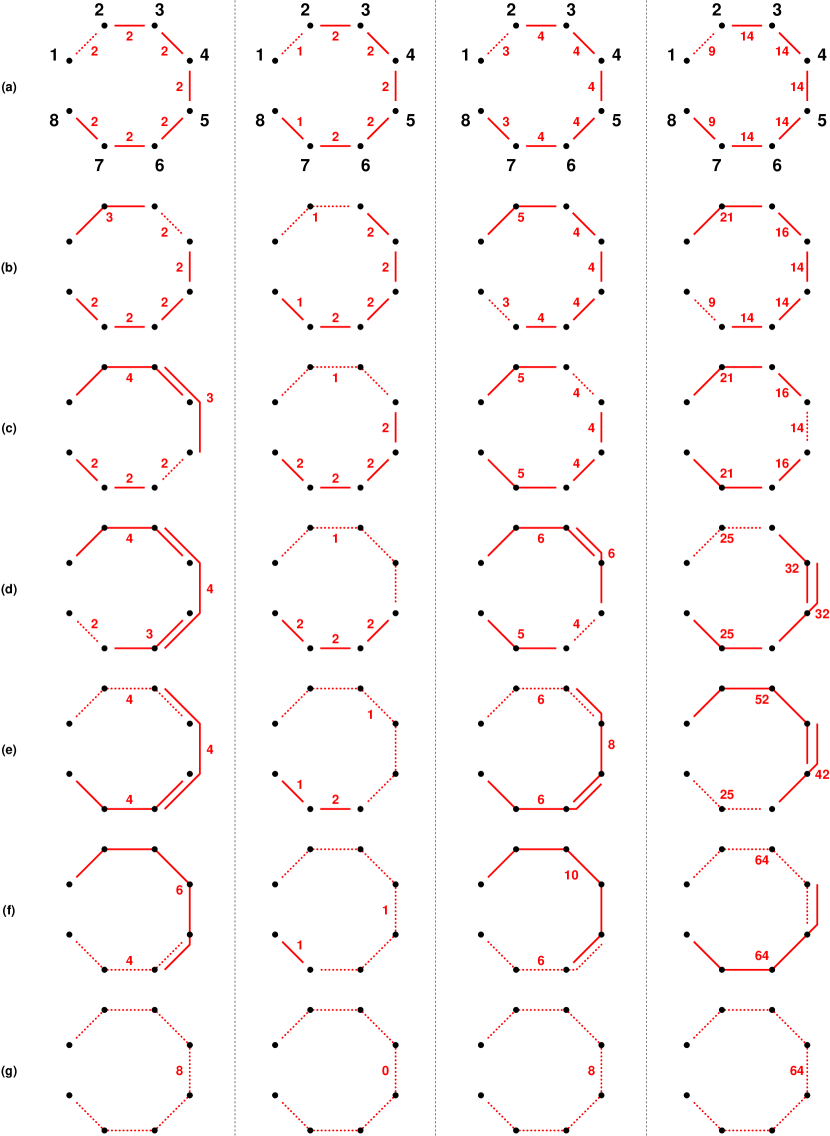
Figure 2: Order of (hyper)edge elimination for a size-$8$ tridiagonal matrix with the strategies (from left to right) Minimal root number (MR, minimize $\mu_{\rm r}(x)$), Minimum incidence (MI, minimize $\mu_{\rm i}(x)$), Minimal roots with look-ahead (MC1, minimize $\mu_{\rm c}^{(1)}(x)$), and Minimal costs with look-ahead (MC2, minimize $\mu_{\rm c}^{(2)}(x)$). For each of the seven elimination steps (a) to (g), the remaining (hyper)edges are shown together with their $\mu$ values, and the (hyper)edge selected for elimination is highlighted as a dotted line. If the minimum is not unique then the “first” minimizing hyperedge (clockwise) is chosen for elimination.

II. Structured graphs

Structured graphs are often encountered in discretizations of partial differential equations. The resulting graphs are planar and usually possess a large diameter. In Figure 3 we report results in terms of accumulated number of roots $\sum|x|$ and cost of root elimination $\sum|x|^{2}$ of the hypergraph edge elimination approach for a uniform $16\times 16$ lattice. We compare the results for the four heuristics with a statistical baseline of $20$ random elimination orderings. As can be seen from the figure all four heuristics yield largely reduced cost measures compared to the baseline. Notably, the ordering of the heuristics in terms of the two cost measures is not identical, i.e., an overall minimal number of accumulated root calculations does not immediately lead to a minimal accumulated root elimination cost.

Figure 3: Accumulated number of roots $\sum|x|$ (top) and root calculation costs $\sum|x|^{2}$ (bottom) for a regular $16\times 16$ lattice graph with $N=256$ nodes. Results for the heuristics are plotted as $(\mu_{\rm i},\triangle)$, $(\mu_{\rm r},\square)$, $(\mu_{\rm c}^{(1)},\circ)$ and $(\mu_{\rm c}^{(2)},\diamond)$ (towards the left), and the boxplots close to the right summarize the results for 20 random elimination orderings.

Next we apply the same test setup to a graph that is a triangulation of the unit disc with $1313$ nodes. In Figure 4 we report accumulated number of roots $\sum|x|$ and root elimination costs $\sum|x|^{2}$ for the four heuristics and report the statistical baseline of $20$ random orderings. Again we see that all four heuristics are clearly better than using a random elimination ordering.

Figure 4: Accumulated number of roots $\sum|x|$ (top) and root calculation costs $\sum|x|^{2}$ (bottom) for a triangulation of the unit disc with $N=1313$ nodes. Results for the heuristics are plotted as $(\mu_{\rm i},\triangle)$, $(\mu_{\rm r},\square)$, $(\mu_{\rm c}^{(1)},\circ)$ and $(\mu_{\rm c}^{(2)},\diamond)$. The boxplots represent results of $20$ random elimination orderings.

III. Sparse random graphs

Finally we compare the heuristics for randomly generated graphs. We use the Matlab built-in function sprandsym to generate an undirected graph with $N$ nodes with a non-zero density of $\tfrac{8}{N}$. The resulting graphs’ average degree is thus approximately $8$. We now test the heuristics for $20$ such graphs of sizes $N=128$. In Figure 5 we report the number of edges of the matrices used in the tests.

Figure 5: Number of edges $|E|$ of $20$ randomly generated sparse graphs.

In Figure 6 we report the results of the heuristics applied to these randomly generated sparse graphs. We report both the accumulated number of roots $\sum|x|$ as well as the accumulated cost of root calculations $\sum|x|^{2}$. In order to gauge the potential gains realized by the heuristics, we include boxplots of $20$ random elimination orderings as well.

Figure 6: Accumulated number of roots $\sum|x|$ (top) and root calculation costs $\sum|x|^{2}$ (bottom) for the $20$ randomly generated sparse graphs. Results for the heuristics are plotted as $(\mu_{\rm i},\triangle)$, $(\mu_{\rm r},\square)$, $(\mu_{\rm c}^{(1)},\circ)$ and $(\mu_{\rm c}^{(2)},\diamond)$. Each boxplot represents results of $20$ random elimination orderings.

Overall, our experiments suggest that, while none of the proposed strategies is consistently superior, choosing the hyperedge with minimum $\mu_{\rm c}^{(1)}$ value for elimination seems to be a reasonable way to reduce both cost measures, the total number of roots to compute, $\sum|x|$, and the operations to do this, $\sum|x|^{2}$.

9 Concluding remarks

We have shown in this paper that the symmetric eigenvalue problem can be interpreted as an elimination process, where all edges of the corresponding graph need to be eliminated. This symbolic equivalence is facilitated by a hypergraph point of view and in complete analogy to the vertex elimination that characterizes the symbolic solution of linear systems by means of Gaussian elimination.

Furthermore, we showed that the hypergraph information in every stage of the elimination process is captured by symbolic Gaussian elimination applied to the edge–edge adjacency matrix—a formal dual to the regular vertex–vertex adjacency matrix. Exploiting this connection we were able to transfer the result of NP-hardness for the calculation of an optimal elimination ordering from the linear systems case to the symmetric eigenvalue problem.

While optimality cannot be achieved, we proposed different heuristics to determine good elimination orderings and numerically explored their use. In particular, we compared them to a baseline of random elimination orderings, where they proved to be vastly superior to this baseline. We also explored if the chosen heuristics are able to reproduce the optimal ordering in case that the graph of the matrix is a chain graph, i.e., the matrix is tri-diagonal. In this case, the proposed edge elimination algorithm with optimal elimination ordering is equivalent to an iterative (rather than recursive) formulation of the divide-and-conquer approach to tridiagonal symmetric eigenvalue problems.

Considered from the point of view of this paper, the usual approach of initial reduction to tridiagonal form and subsequent solution of the tridiagonal eigenvalue problem can be viewed as the reduction to a chain graph with subsequent edge elimination, for which an optimal elimination strategy is known.

The equivalence of the Hermitian eigenvalue problem and symbolic hypergraph edge elimination can be easily transferred to the calculation of the singular value decompostion based on the observation the the singular value decompostion $AV=U\Sigma$ of $A\in\mathbb{C}^{m\times n}$ can be computed by considering the Hermitian eigenvalue problem

$$\begin{bmatrix}0&A^{H}\\ A&0\end{bmatrix}\begin{bmatrix}V&V\\ U&-U\end{bmatrix}=\begin{bmatrix}V&V\\ U&-U\end{bmatrix}\begin{bmatrix}\Sigma&0\\ 0&-\Sigma\end{bmatrix}.$$

References

- [1] E. Anderson, Z. Bai, C. Bischof, S. Blackford, J. Demmel, J. Dongarra, J. Du Croz, A. Greenbaum, S. Hammarling, A. McKenney, and D. Sorensen, LAPACK Users’ Guide, SIAM, Philadelphia, PA, 3rd ed., 1999.
- [2] T. Auckenthaler, V. Blum, H.-J. Bungartz, T. Huckle, R. Johanni, L. Krämer, B. Lang, H. Lederer, and P. R. Willems, Parallel solution of partial symmetric eigenvalue problems from electronic structure calculations, Parallel Comput., 37 (2011), pp. 783–794.
- [3] J. R. Bunch, C. P. Nielsen, and D. C. Sorensen, Rank-one modification of the symmetric eigenproblem, Numer. Math., 31 (1978), pp. 31–48.
- [4] J. J. M. Cuppen, A divide and conquer method for the symmetric tridiagonal eigenproblem, Numer. Math., 36 (1981), pp. 177–195.
- [5] T. A. Davis, Direct Methods for Sparse Linear Systems, SIAM, Philadelphia, PA, 2006.
- [6] J. W. Demmel, Applied Numerical Linear Algebra, SIAM, Philadelphia, PA, 1997.
- [7] J. J. Dongarra and D. C. Sorensen, A fully parallel algorithm for the symmetric eigenvalue problem, SIAM J. Sci. Stat. Comput., 8 (1987), pp. s139–s154.
- [8] F. R. Gantmacher and M. G. Kreĭn, Oszillationsmatrizen, Oszillationskerne und kleine Schwingungen mechanischer Systeme, no. 2 in Mathematische Lehrbücher und Monographien: 1. Abteilung, mathematische Lehrbücher, Akad.-Verlag, 1960.
- [9] A. George and J. W. Liu, Computer Solution of Large Sparse Positive Definite Systems, Prentice Hall, Englewood Cliffs, NJ, 1981.
- [10] G. H. Golub, Some modified matrix eigenvalue problems, SIAM Rev., 15 (1973), pp. 318–334.
- [11] M. Gu and S. C. Eisenstat, A stable and efficient algorithm for the rank-one modification of the symmetric eigenproblem, SIAM J. Matrix Anal. Appl., 15 (1994), pp. 1266–1276.
- [12] J. H. Wilkinson, The Algebraic Eigenvalue Problem, Clarendon Press, Oxford, 1965.
- [13] M. Yannakakis, Computing the minimum fill-in is NP-complete, SIAM J. Alg. Disc. Meth., 2 (1981), pp. 77–79.
- [14] A. A. Zykov, Hypergraphs, Russian Math. Surveys, 29 (1974), pp. 89–156.