Abstract

In the emerging field of 3D bioprinting, cell damage due to large deformations is considered a main cause for cell death and loss of functionality inside the printed construct. Those deformations, in turn, strongly depend on the mechano-elastic response of the cell to the hydrodynamic stresses experienced during printing. In this work, we present a numerical model to simulate the deformation of biological cells in arbitrary three-dimensional flows. We consider cells as an elastic continuum according to the hyperelastic Mooney–Rivlin model. We then employ force calculations on a tetrahedralized volume mesh.

To calibrate our model, we perform a series of FluidFM^®  compression experiments with REF52 cells demonstrating that all three parameters of the Mooney–Rivlin model are required for a good description of the experimental data at very large deformations up to $80\text{\,}\mathrm{\char 37\relax}$. In addition, we validate the model by comparing to previous AFM experiments on bovine endothelial cells and artificial hydrogel particles. To investigate cell deformation in flow, we incorporate our model into Lattice Boltzmann simulations via an Immersed-Boundary algorithm. In linear shear flows, our model shows excellent agreement with analytical calculations and previous simulation data.

Keywords: Hyperelasticity, Cell deformation, Mooney–Rivlin, Atomic force Microscopy, Shear flow, Lattice-Boltzmann

1 Introduction

The dynamic behavior of flowing cells is central to the functioning of organisms and forms the base for a variety of biomedical applications. Technological systems that make use of the elastic behavior of cells are, for example, cell sorting [1], real-time deformability cytometry [2, 3] or probing techniques for cytoskeletal mechanics [4, 5, 6, 7, 8, 9, 10, 11, 12, 13, 14, 15]. In most, but not all, of these applications cell deformations typically remain rather small. A specific example where large deformations become important is 3D bioprinting. Bioprinting is a technology which, analogously to common 3D printing, pushes a suspension of cells in highly viscous hydrogels—a so-called bioink—through a fine nozzle to create three-dimensional tissue structures. A major challenge in this process lies in the control of large cell deformations and cell damage during printing. Those deformations arise from hydrodynamic stresses in the printer nozzle and ultimately affect the viability and functionality of the cells in the printed construct [16, 17, 18, 19, 20]. How exactly these hydrodynamic forces correlate with cell deformation, however, strongly depends on the elastic behavior of the cell and its interaction with the flowing liquid. Theoretical and computational modeling efforts in this area have thus far been restricted to pure fluid simulations without actually incorporating the cells [21, 22, 17] or simple 2D geometries [23, 24]. The complexity of cell mechanics and the diversity of possible applications make theoretical modeling of cell mechanics in flow a challenge which, to start with, requires reliable experimental data for large cell deformations.

The most appropriate tool to measure cellular response at large deformations is atomic force microscopy (AFM) [25, 26, 27, 28, 8, 29, 30, 31, 32, 33, 34]. AFM cantilevers with pyramidal tips, colloidal probes, or flat geometries are used to indent or compress cells. Therefore, a common approach to characterize the elasticity of cells utilizes the Hertzian theory, which describes the contact between two linear elastic solids [35, p. 90-104], but is limited to the range of small deformations [36]. Experimental measurements with medium-to-large deformations typically show significant deviations from the Hertz prediction, e. g., for cells or hydrogel particles [37]. Instead of linear elasticity, a suitable description of cell mechanics for bioprinting applications requires more advanced hyperelastic material properties. While for simple anucleate fluid-filled cells such as, e.g., red blood cells, theoretical models abound [38, 39, 40, 41, 42], the availability of models for cells including a complex cytoskeleton is rather limited. In axisymmetric geometries, Caille et al. [43] and Mokbel et al. [44] used an axisymmetric finite element model with neo-Hookean hyperelasticity to model AFM and microchannel experiments on biological cells. In shear flow, approximate analytical treatments are possible [45, 46, 47, 48]. Computationally, Gao and Hu [46] carried out 2D simulations while in 3D Lykov et al. [49] utilized a DPD technique based on a bead-spring model. Furthermore, Villone et al. [50, 51] presented an arbitrary Lagrangian-Eulerian approach for elastic particles in viscoelastic fluids. Finally, Rosti et al. [52] and Saadat et al. [53] considered viscoelastic and neo-Hookean finite element models, respectively, in shear flow.

In this work, we introduce and calibrate a computational model for fully three-dimensional simulations of cells in arbitrary flows. Our approach uses a Lattice-Boltzmann solver for the fluid and a direct force formulation for the elastic equations. In contrast to earlier works [43, 47, 44, 52, 53] our model uses a three-parameter Mooney–Rivlin elastic energy functional. To demonstrate the need for this more complex elastic model, we carry out extensive FluidFM^®  indentation experiments for REF52 (rat embryonic fibroblast) cells at large cell deformation up to $80\text{\,}\mathrm{\char 37\relax}$ [54]. In addition, our model compares favorably with previous AFM experiments on bovine endothelial cells [43] as well as artificial hydrogel particles [37]. Our model provides a much more realistic force–deformation behavior compared to the small-deformation Hertz approximation, but is still simple and fast enough to allow the simulation of dense cell suspensions in reasonable time. Particularly, our approach is less computationally demanding than conventional finite-element methods which usually require large matrix operations. Furthermore, it is easily extensible and allows, e.g., the inclusion of a cell nucleus by the choice of different elastic moduli for different parts of the volume.

We finally present simulations of our cell model in different flow scenarios using an Immersed-Boundary algorithm to couple our model with Lattice Boltzmann fluid calculations. In a plane Couette (linear shear) flow, we investigate the shear stress dependency of single cell deformation, which we compare to the average cell deformation in suspensions with higher volume fractions, and show that our results in the neo-Hookean limit are in accordance with earlier elastic cell models [47, 52, 53].

2 Theory

In general, hyperelastic models are used to describe materials that respond elastically to large deformations [55, p. 93]. Many cell types can be subjected to large reversible shape changes. This section provides a brief overview of the hyperelastic Mooney–Rivlin model implemented in this work.

The displacement of a point is given by

$$u_{i}=y_{i}-x_{i}\>,$$ (1)

where $x_{i}$ ($i=1,2,3$) refers to the undeformed configuration (material frame) and $y_{i}$ to the deformed coordinates (spatial frame). We define the deformation gradient tensor and its inverse as [55, p. 14,18]

$$\mathsf{F}_{ij}=\frac{\partial{y_{i}}}{\partial{x_{j}}}=\frac{\partial{u_{i}}}{\partial{x_{j}}}+\delta_{ij}\quad\mathrm{and}\quad\mathsf{F}_{ij}^{-1}=\frac{\partial{x_{i}}}{\partial{y_{j}}}\>.$$ (2)

Together with the right Cauchy-Green deformation tensor, $\mathsf{C}=\mathsf{F}^{\intercal}\mathsf{F}$ (material description), we can define the following invariants which are needed for the strain energy density calculation below:

$$J =\det\mathsf{F}$$ (3)

$$I =T_{\mathsf{C}}J^{-2/3}$$ (4)

$$K =\tfrac{1}{2}\left(T_{\mathsf{C}}^{2}-T_{\mathsf{C}^{2}}\right)J^{-4/3}$$ (5)

Here,

$$T_{\mathsf{C}}=\mathrm{tr}\,\mathsf{C}\quad\mathrm{and}\quad T_{\mathsf{C}^{2}}=\mathrm{tr}\,\left(\mathsf{C}^{2}\right)$$ (6)

are the trace of the right Cauchy-Green deformation tensor and its square, respectively. The nonlinear strain energy density of the Mooney–Rivlin model is given by [56, 57]

$$U=\left[\frac{\mu_{1}}{2}\left(I-3\right)+\frac{\mu_{2}}{2}\left(K-3\right)+\frac{\kappa}{2}\left(J-1\right)^{2}\right]\>,$$ (7)

where $\mu_{1}$, $\mu_{2}$, and $\kappa$ are material properties. They correspond—for consistency with linear elasticity in the range of small deformations—to the shear modulus $\mu=\mu_{1}+\mu_{2}$ and bulk modulus $\kappa$ of the material and are therefore related to the Young’s modulus $E$ and the Poisson ratio $\nu$ via [55, p. 74]

$$\mu=\frac{E}{2\left(1+\nu\right)}\quad\mathrm{and}\quad\kappa=\frac{E}{3\left(1-2\nu\right)}\>.$$ (8)

Through the choice $\mu_{2}=0$ in (7), we recover the simpler and frequently used [47, 53] neo-Hookean strain energy density:

$$U_{\mathrm{NH}}=\left[\frac{\mu}{2}\left(I-3\right)+\frac{\kappa}{2}\left(J-1\right)^{2}\right]$$ (9)

As we show later, this can be a sufficient description for some cell types. To control the strength of the second term and quickly switch between neo-Hookean and Mooney–Rivlin strain energy density calculation, we introduce a factor $w\in\left[0,1\right]$ and set

$$\mu_{1}=w\mu\quad\mathrm{and}\quad\mu_{2}=(1-w)\mu\>$$ (10)

such that $w=1$, which equals setting $\mu_{2}=0$ in (7), corresponds to the purely neo-Hookean description in (9), while $w<1$ increases the influence of the $\mu_{2}$-term and thus leads to a more pronounced strain hardening as shown in figure S-6 of the Supporting Information.

3 Tetrahedralized cell model

In this section we apply the hyperelastic theory of section 2 to a tetrahedralized mesh as shown in figure 1.

3.1 Calculation of elastic forces

We consider a mesh consisting of tetrahedral elements as depicted in figure 1. The superscript $\alpha$ refers to the four vertices of the tetrahedron. The elastic force acting on vertex $\alpha$ in direction $i$ is obtained from (7) by differentiating the strain energy density $U$ with respect to the vertex displacement as

$$f_{i}^{\alpha}= -V_{0}\frac{\partial{U}}{\partial{u_{i}^{\alpha}}}\>,$$ (11)

where $V_{0}$ is the reference volume of the tetrahedron. In contrast to Saadat et al. [53], the numerical calculation of the force in our model does not rely on the integration of the stress tensor, but on a differentiation where the calculation of all resulting terms involves only simple arithmetics. Applying the chain rule for differentiation yields:

$$f_{i}^{\alpha}=-V_{0}\Bigg{[} \left(\frac{\partial{U}}{\partial{I}}\frac{\partial{I}}{\partial{T_{\mathsf{C}}}}+\frac{\partial{U}}{\partial{K}}\frac{\partial{K}}{\partial{T_{\mathsf{C}}}}\right)\frac{\partial{T_{\mathsf{C}}}}{\partial{\mathsf{F}_{kl}}}$$

$$+\left(\frac{\partial{U}}{\partial{I}}\frac{\partial{I}}{\partial{J}}+\frac{\partial{U}}{\partial{K}}\frac{\partial{K}}{\partial{J}}+\frac{\partial{U}}{\partial{J}}\right)\frac{\partial{J}}{\partial{\mathsf{F}_{kl}}}$$

$$+\frac{\partial{U}}{\partial{K}}\frac{\partial{K}}{\partial{T_{\mathsf{C}^{2}}}}\frac{\partial{T_{\mathsf{C}^{2}}}}{\partial{\mathsf{F}_{kl}}}\Bigg{]}\frac{\partial{\mathsf{F}_{kl}}}{\partial{u_{i}^{\alpha}}}$$ (12)

The evaluation of (3.1) requires the calculation of the deformation gradient tensor $\mathsf{F}$, which is achieved by linear interpolation of the coordinates and displacements inside each tetrahedral mesh element as detailed in the next section. We note that our elastic force calculation is purely local making it straightforward to employ different elastic models in different regions of the cell and/or to combine it with elastic shell models. This flexibility can be used to describe, e.g., the cell nucleus [43] or an actin cortex [58] surrounding the cell interior.

3.2 Interpolation of the displacement field

Following standard methods, e.g. Bower [55], we start by interpolating a point $x_{i}$ inside a single tetrahedron using the vertex positions $x_{i}^{\alpha}$ ($\alpha=1,2,3,4$). The interpolation uses an inscribed, dimensionless coordinate system, denoted by $\left(\xi_{1},\xi_{2},\xi_{3}\right)$ with $0\leq\xi_{i}\leq 1$, as depicted in figure 1a. One vertex defines the origin while the remaining three indicate the coordinate axes. A set of shape functions, i. e., interpolation functions, $N^{\alpha}\left(\xi_{1},\xi_{2},\xi_{3}\right)$ is employed to interpolate positions inside the tetrahedron volume. An arbitrary point $x_{i}$ inside the element is interpolated as

$$x_{i}=\sum\limits_{\alpha=1}^{4}N^{\alpha}\left(\xi_{1},\xi_{2},\xi_{3}\right)x_{i}^{\alpha}\>,$$ (13)

where the shape functions are defined as [55, p. 483]:

$$N^{1}\left(\xi_{1},\xi_{2},\xi_{3}\right) =\xi_{1}$$ (14)

$$N^{2}\left(\xi_{1},\xi_{2},\xi_{3}\right) =\xi_{2}$$ (15)

$$N^{3}\left(\xi_{1},\xi_{2},\xi_{3}\right) =\xi_{3}$$ (16)

$$N^{4}\left(\xi_{1},\xi_{2},\xi_{3}\right) =1-\xi_{1}-\xi_{2}-\xi_{3}$$ (17)

According to (1), the displacement of vertex $\alpha$ in $i$-direction is given by

$$u_{i}^{\alpha}=y_{i}^{\alpha}-x_{i}^{\alpha}\>.$$ (18)

Therefore similar to (13), the displacement at an arbitrary point in the volume can also be expressed in terms of the shape functions and the vertex displacements as

$$u_{i}=\sum\limits_{\alpha=1}^{4}N^{\alpha}\left(\xi_{1},\xi_{2},\xi_{3}\right)u_{i}^{\alpha}\>.$$ (19)

The calculation of the deformation gradient tensor according to (2) requires the spatial derivative of the displacement:

$$\mathsf{F}_{ij}-\delta_{ij}=\frac{\partial{u_{i}}}{\partial{x_{j}}} =\frac{\partial{u_{i}}}{\partial{\xi_{k}}}\frac{\partial{\xi_{k}}}{\partial{x_{j}}}=\mathsf{A}_{ik}\mathsf{B}_{kj}$$ (20)

By inserting (19) into (20) and evaluating the shape functions, the components of the matrix $\mathsf{A}$ are easily determined to be the difference of the displacements between the origin (vertex 4) and the remaining vertices 1, 2 and 3:

$$\mathsf{A}_{ik}=u_{i}^{k}-u_{i}^{4}$$ (21)

Note that due to the linear interpolation $\mathsf{A}_{ik}$ is constant inside a given tetrahedron. The matrix $\mathsf{B}=\mathsf{\mathsf{J}}^{-1}$ is the inverse of the Jacobian matrix, obtained similarly to (21) as

$$\mathsf{J}_{ik} =\frac{\partial{x_{i}}}{\partial{\xi_{k}}}=x_{i}^{k}-x_{i}^{4}\>.$$ (22)

Since $x_{i}$ refers to the reference coordinates, the calculation of the matrices $\mathsf{\mathsf{J}}$ and $\mathsf{B}$ has to be performed only once at the beginning of a simulation. With the interpolation of the displacement in each tetrahedron, we can write all derivatives occurring in (3.1), as listed in the following:
$\frac{\partial{U}}{\partial{I}}=\frac{\mu_{1}}{2}$ $\frac{\partial{I}}{\partial{T_{\mathsf{C}}}}=J^{-\frac{2}{3}}$ $\frac{\partial{U}}{\partial{K}}=\frac{\mu_{2}}{2}$ $\frac{\partial{K}}{\partial{T_{\mathsf{C}}}}=T_{\mathsf{C}}J^{-\frac{4}{3}}$ $\frac{\partial{T_{\mathsf{C}}}}{\partial{\mathsf{F}_{il}}}=2\mathsf{F}_{il}$ $\frac{\partial{I}}{\partial{J}}=-\frac{2}{3}T_{\mathsf{C}}J^{-\frac{5}{3}}$ $\frac{\partial{K}}{\partial{J}}=-\frac{2}{3}\left(T_{\mathsf{C}}^{2}-T_{\mathsf{C}^{2}}\right)J^{-\frac{7}{3}}$ $\frac{\partial{U}}{\partial{J}}=\kappa\left(J-1\right)$ $\frac{\partial{J}}{\partial{\mathsf{F}_{il}}}=J\mathsf{F}_{li}^{-1}$ $\frac{\partial{K}}{\partial{T_{\mathsf{C}^{2}}}}=-\tfrac{1}{2}J^{-\frac{4}{3}}$ $\frac{\partial{T_{\mathsf{C}^{2}}}}{\partial{\mathsf{F}_{il}}}=4\mathsf{F}_{ik}\mathsf{C}_{kl}$ $\frac{\partial{\mathsf{F}_{kl}}}{\partial{u_{i}^{\alpha}}}=\delta_{ki}\mathsf{B}_{ml}\left(\delta_{m\alpha}-\delta_{4\alpha}\right)$

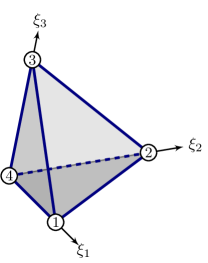
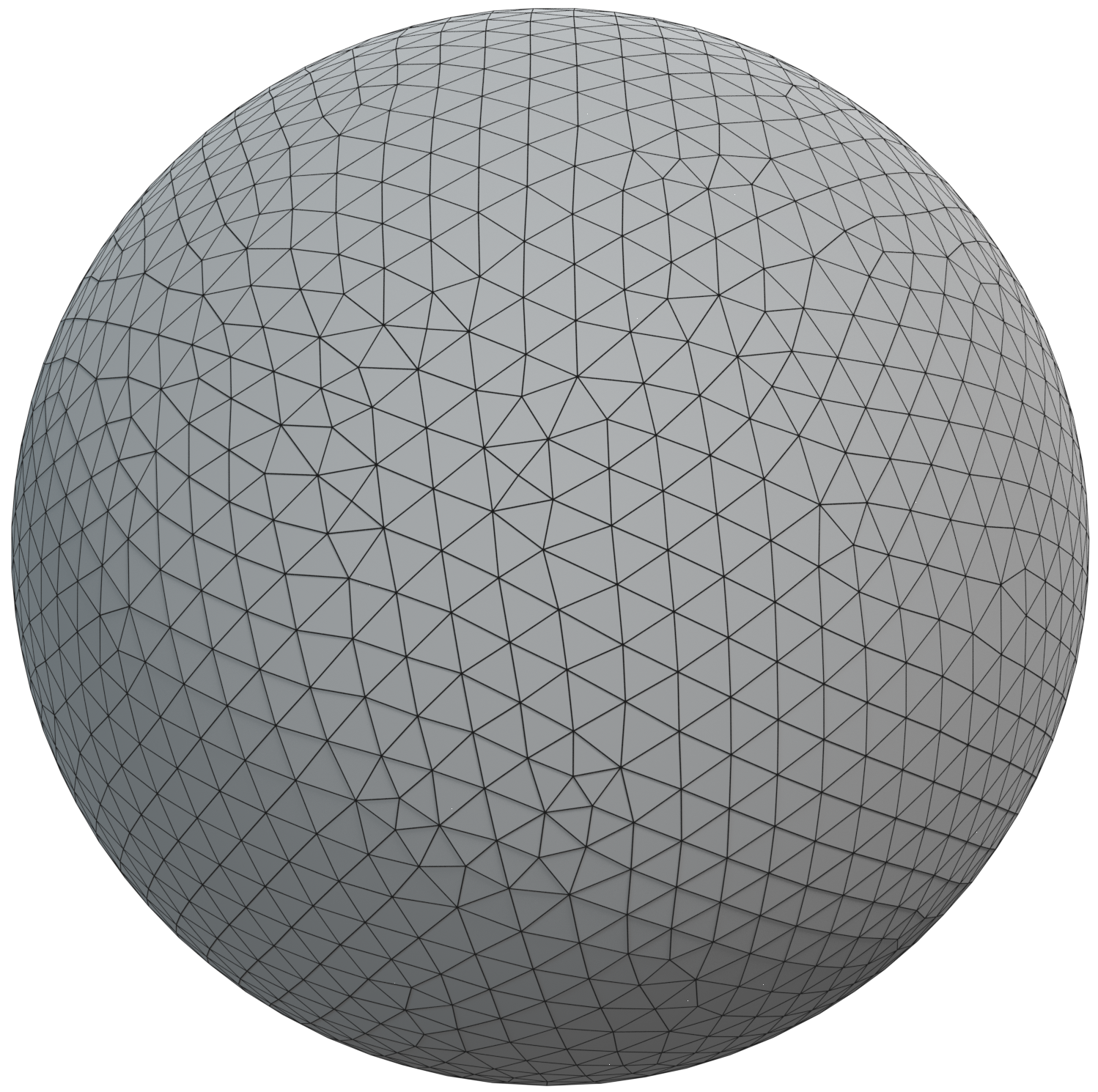
(a)   (b)   (c)

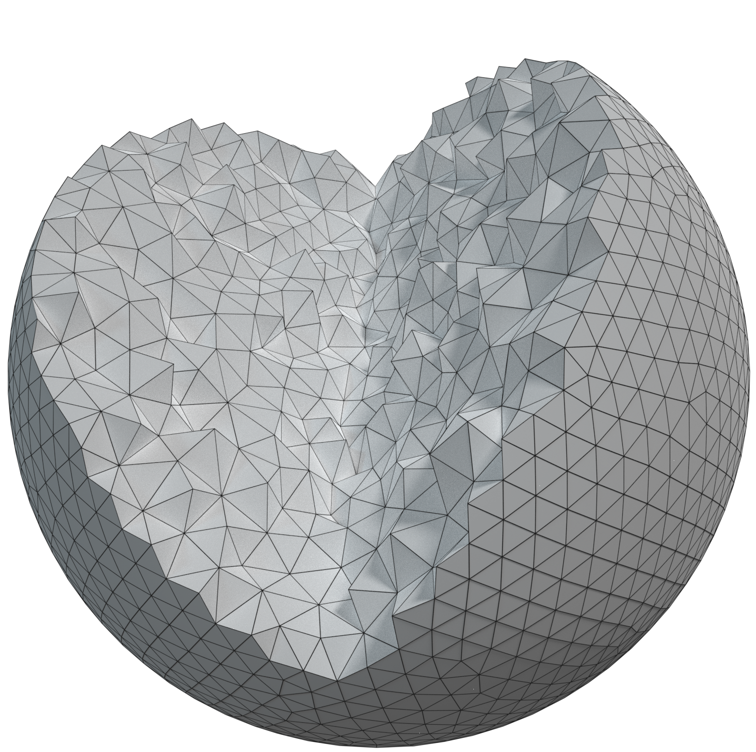
Figure 1: (a) The four noded tetrahedron as mesh element within a local dimensionless coordinate system $\left\{\xi_{1},\xi_{2},\xi_{3}\right\}$. (b) The spherical cell model with its triangulated surface and (c) its inner tetrahedralized mesh

3.3 Taylor deformation parameter

As a measure for the cell deformation, we use the Taylor deformation parameter [59, 60, 61, 53]

$$D=\frac{a_{3}-a_{1}}{a_{3}+a_{1}}\>,$$ (23)

where $a_{1}$ and $a_{3}$ are respectively the minor and major semi axis of an ellipsoid corresponding to the inertia tensor of the cell. The Taylor deformation is a good measure for approximately elliptic cell deformations, as they occur in shear flow (cf. section 6).

To calculate $D$, first the components of the inertia tensor

$$\mathsf{\Theta}_{ij}=\int\limits_{V}x_{k}x_{k}\delta_{ij}-x_{i}x_{j}{\mathrm{d}{V}}\>,$$ (24)

where $\vec{x}$ is a vector inside the volume $V$, are calculated using our discretized cell with $N_{\mathrm{tet}}$ tetrahedra as

$$\mathsf{\Theta}_{ij}=\sum\limits_{l=1}^{N_{\mathrm{tet}}}V_{l}\left(r_{k}^{l}r_{k}^{l}\delta_{ij}-r_{i}^{l}r_{j}^{l}\right)\>.$$ (25)

The vector $\vec{r}^{\,l}$ denotes the center of mass of the $l^{\mathrm{th}}$ tetrahedron and $V_{l}$ is its current volume. The eigenvalues $\theta_{1}>\theta_{2}>\theta_{3}$ of $\mathsf{\Theta}$ can be used to fit the semi axes $a_{1}<a_{2}<a_{3}$ of the corresponding ellipsoid:

$$a_{1} =\frac{5}{2M}\left(-\theta_{1}+\theta_{2}+\theta_{3}\right)$$

$$a_{2} =\frac{5}{2M}\left(\theta_{1}-\theta_{2}+\theta_{3}\right)$$

$$a_{3} =\frac{5}{2M}\left(\theta_{1}+\theta_{2}-\theta_{3}\right)$$ (26)

The prefactor contains the mass $M$ of the ellipsoid (considering uniform mass density) and drops out in the calculation of $D$.

4 Comparison of the numerical model to FluidFM^®  measurements on REF52 cells

In this section, we validate compression simulations of our cell model with FluidFM^®  compression experiments of REF52 cells stably expressing paxillin-YFP [54]. These experiments provide as an output the required force to produce a certain deformation of the cell, which can be directly compared to our model. We start with a detailed description of the experiments and show the suitability of our model to describe the elastic behavior of REF52 cells afterwards.

4.1 FluidFM^®  indentation measurements

We perform a series of compression measurements of REF52 cells with a Flex FPM (Nanosurf GmbH, Germany) system that combines the AFM with the FluidFM^®  technology (Cytosurge AG, Switzerland). In contrast to conventional AFM techniques, FluidFM^®  uses flat cantilevers that possess a microchannel connected to a pressure system. By applying a suction pressure, cells can be aspirated and retained at the aperture of the cantilever’s tip. A more detailed description of the setup and its functionality is already reported in [31]. All experiments are based on a cantilever with an aperture of $8\text{\,}\mathrm{\SIUnitSymbolMicro m}$ diameter and a nominal spring constant of $2\text{\,}\mathrm{N}\text{\,}{\mathrm{m}}^{-1}$. In order to measure the cellular deformation, a cell was sucked onto the tip and compressed between the cantilever and the substrate until a setpoint of $100\text{\,}\mathrm{nN}$ was reached. Immediately before the experiment, the cells were detached by using Accutase (Sigma Aldrich) and were therefore in suspension at the time of indentation. In this way, it can be ensured that only a single cell is deformed during each measurement.

An example micrograph of the experiment before compression is shown in figure 2. Analogously to AFM, primary data in form of cantilever position (in $\mathrm{m}$) and deflection (in $\mathrm{V}$) has to be converted to force and deformation through the deflection sensitivity (in $\mathrm{m}\text{\,}{\mathrm{V}}^{-1}$) and the cantilevers’ spring constant. The cellular deformation further requires the determination of the contact point, which we choose as the cantilever position where the measured force starts to increase. The undeformed cell size is obtained as mean from a horizontal and vertical diameter measurement using the software imageJ.

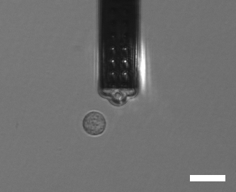
Figure 2: Example micrograph showing the FluidFM^®  cantilever and a cell viewed from the top. Scale bar is $30\text{\,}\mathrm{\SIUnitSymbolMicro m}$

4.2 Simulation setup

The experimental setup of the previous section is easily transferred and implemented for our cell model: the undeformed spherical cell rests on a fixed plate while a second plate approaches from above to compress the cell as depicted in figure 3 (a and b). In section 5.2 below we will also use a slightly modified version where a sphere indents the cell as shown in figure 3 (c and d). A repulsive force prevents the cell vertices from penetrating the plates or the spherical indenter. The elastic restoring forces (cf. section 3) acting against this imposed compression are transmitted throughout the whole mesh, deforming the cell.

We use meshes consisting of $2000$ to $5000$ vertices and about $10\,000$ to $30\,000$ tetrahedra to build up a spherical structure. More details of the mesh and its generation (section S-2.4) as well as the algorithm (section S-3) are provided in the SI.

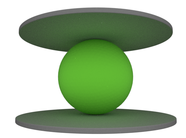
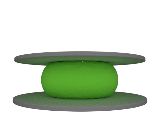
(a) (b) (c) (d)

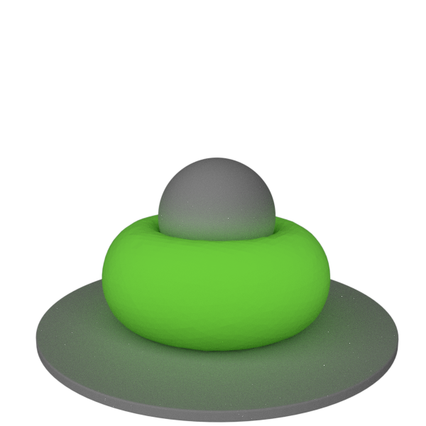
Figure 3: (a and b) Cell compression simulations: The cell is compressed between a lower, resting, and an upper, moving, plate. (c and d) Colloidal probe cell indentation simulations: The cell rests on a plate, while being indented with a sphere

4.3 Results

In our FluidFM^®  experiment series with REF52 cells, the cell radii lie between $7.1\text{\,}\mathrm{\SIUnitSymbolMicro m}$ and $10.4\text{\,}\mathrm{\SIUnitSymbolMicro m}$ with an overall average of $8.6(7)\text{\,}\mathrm{\SIUnitSymbolMicro m}$. In figure 4 we depict the force as function of the non-dimensionalized deformation, i. e., the absolute compression divided by the cell diameter. The experimental data curves share general characteristics: The force increases slowly in the range of small deformations up to roughly $40\text{\,}\mathrm{\char 37\relax}$, while a rapidly increasing force is observed for larger deformations. Although the variation of the cell radius in the different measurements is already taken into account in the deformation, the point of the force upturn differs significantly which indicates a certain variability in the elastic parameters of the individual cells.

We use the compression simulation setup as detailed in section 4.2 to calculate force–deformation curves of our cell model. The Poisson ratio is chosen as $\nu=0.48$. In section S-2.7 of the Supporting Information we show that variations of the $\nu$ do not strongly affect the results. A best fit approach is used to determine the Young’s modulus and the ratio of shear moduli $w$ and leads to very good agreement between model prediction and experimental data as shown in figure 4 as well as section S-1 of the SI. While the general range of force values is controlled using the Young’s modulus, the Mooney–Rivlin ratio $w$ especially defines the point of the force upturn. We find Young’s moduli in the range $110\text{\,}\mathrm{Pa}$ to $160\text{\,}\mathrm{Pa}$ and $w=0.25$, $0.5$, and $1$. For very small deformations our hyperelastic model produces the same results as would be expected from a linear elastic model according to the Hertz theory. See the SI (section S-2.5) for further details on the calculation of the force–deformation according to the Hertzian theory. For large deformations, the force rapidly increases due to its nonlinear character, showing strain-hardening behavior and huge deviations from the Hertz theory. Overall, we find an excellent match between simulation and our FluidFM^®  measurements with REF52 cells.

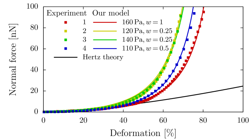
Figure 4: Our numerical model in comparison to our FluidFM^®  measurements on REF52 cells. The labels give the two fit parameters $E$ and $w$. We find Young’s moduli in the range of $110\text{\,}\mathrm{Pa}$ to $160\text{\,}\mathrm{Pa}$. The Hertz theory is shown for a Young’s modulus of $180\text{\,}\mathrm{Pa}$

5 Comparison of our numerical model to other micromechanical setups

In this section, we compare our simulations to axisymmetric calculations using the commercial software Abaqus and validate our cell model with further experimental data for bovine endothelial cells from [43] and very recent data for hydrogel particles from [37].

5.1 Validation with axisymmetric simulations

To validate our model numerically, we compare our simulated force–deformation curves to calculations using the commercial software Abaqus [62] (version 6.14).

In Abaqus, we use a rotationally symmetric setup consisting of a two-dimensional semicircle, which is compressed between two planes, similar to our simulation setup in section 4.2 and the finite element model utilized in [43]. The semicircle has a radius $r=$15\text{\,}\mathrm{\SIUnitSymbolMicro m}$$, a Young’s modulus of $E=$2.25\text{\,}\mathrm{kPa}$$ and a Poisson ratio of $\nu=0.48$. We choose a triangular mesh and the built-in implementation of the hyperelastic neo-Hookean model. In figure 5 we see very good agreement between the results of the two different numerical methods.

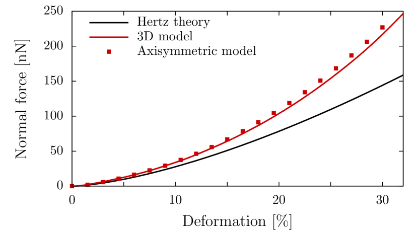
Figure 5: Comparison of force–deformation curves obtained from our model (red line) with the linear elastic Hertz theory (black line) and the two-dimensional simulation with Abaqus (red squares), showing good agreement between our three-dimensional and the axisymmetric model

5.2 Validation with AFM experiments

To compare with the AFM experiments of Caille et al. [43], we simulate a cell with radius $15\text{\,}\mathrm{\SIUnitSymbolMicro m}$ using the setup of section 4.2. For the hydrogel particle indentation [37] we use the setup depicted in figure 3 (c and d) with a particle radius of $40\text{\,}\mathrm{\SIUnitSymbolMicro m}$ and a radius of the colloidal probe of $26.5\text{\,}\mathrm{\SIUnitSymbolMicro m}$. The Poisson ratio is chosen as $0.48$ in all simulations and the Young’s modulus is determined using a best fit to the experimental data points. Since the neo-Hookean description appears to be sufficient for these data sets, we further set $w=1$.

In figure 6a, we show the experimental data for suspended, round, bovine endothelial cells of five separate measurements from [43] together with the prediction of the Hertz theory for a Young’s modulus of $1000\text{\,}\mathrm{Pa}$. Fitting our data with Young’s moduli in the range of $550\text{\,}\mathrm{Pa}$ to $2400\text{\,}\mathrm{Pa}$, we find good agreement between our calculations and the experimental data. We note that Caille et al. [43] observed similarly good agreement for their axisymmetric incompressible neo-Hookean FEM simulations which, however, cannot be coupled to external flows in contrast to the approach presented here. The same procedure is applied to the colloidal probe indentation data of hydrogel particles from [37], showing in figure 6b the experimental data and the prediction of the Hertz theory from [37]. We find excellent agreement between our model calculations for Young’s moduli in the range of $$580$\pm$100\text{\,}\mathrm{Pa}$$ and the experimental data. For both systems, figure 6 shows large deviations between the Hertzian theory and the experimental data for medium-to-large deformations. Our model provides a significant improvement in this range.

(a)
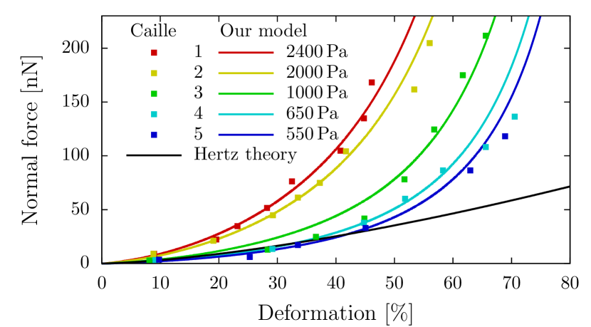
(b)

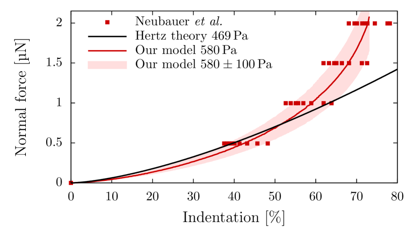
Figure 6: (a) Our numerical model in comparison to experimental measurements of bovine endothelial cells from [43]. The black line depicts the prediction of the Hertz theory for a Young’s modulus of $1000\text{\,}\mathrm{Pa}$. (b) Our numerical model in comparison to experimental measurements of hydrogel particles from [37]. The indicated range corresponds to the experimentally found range of $\pm$100\text{\,}\mathrm{Pa}$$ for the Young’s modulus according to the depicted Hertz model

6 Application in shear flow

We now apply our model to study the behavior of cells in a plane Couette (linear shear) flow setup and compare the steady cell deformation to other numerical and analytical cell models of Gao et al. [47], Rosti et al. [52] and Saadat et al. [53]. A sketch of the simulation setup is shown in figure 7. For simplicity, we choose $w=1$ to reduce the Mooney–Rivlin description (7) to two free parameters $\mu$ and $\kappa$ (or $E$ and $\nu$), obtaining a compressible neo-Hookean form. We use the Lattice Boltzmann implementation of the open source software package ESPResSo [63, 64]. Coupling between fluid and cell is achieved via the immersed-boundary algorithm [65, 53] which we implemented into ESPResSo [66, 58]. We note here that, in contrast to Saadat et al. [53], we do not subtract the fluid stress within the particle interior. This leads to a small viscous response of the cell material in addition to its elasticity. To obtain (approximately) the limit of a purely elastic particle, we exploit a recently developed method by Lehmann et al. [67] to discriminate between the cell interior and exterior during the simulation. Using this technique, we can tune the ratio between inner and outer viscosity $\lambda$ with $\lambda\to 0$ representing a purely elastic particle. For simplicity, we will nevertheless set $\lambda=1$ in the following, except where otherwise noted. Details of the method are provided in the SI (section S-4.1). As measure for the deformation, we investigate the Taylor parameter $D$ (23) of our initially spherical cell model in shear flow at different shear rates $\dot{\gamma}$.

6.1 Single cell simulation

The first simulation setup, a single cell in infinite shear flow, is realized by choosing a simulation box of the dimensions $10\times 15\times 5$ ($x\times y\times z$) in units of the cell radius. The infinite shear flow is approximated by applying a tangential velocity $u_{\mathrm{wall}}$ on the $x$-$z$-planes at $y=0$ in negative and at $y=15$ in positive $x$-direction, as depicted in figure 7. The tangential wall velocity is calculated using the distance $H$ of the parallel planes and the constant shear rate $\dot{\gamma}$ via

$$u_{\mathrm{wall}}=\tfrac{1}{2}H\dot{\gamma}\>.$$ (27)

The box is periodic in $x$ and $z$. A single cell is placed at the center of the simulation box corresponding to a volume fraction of $\phi=0.0003$. We choose the following parameters: fluid mass density $\varrho=${10}^{3}\text{\,}\mathrm{kg}\text{\,}{\mathrm{m}}^{-3}$$, dynamic viscosity $\eta=${10}^{-3}\text{\,}\mathrm{Pa}\text{\,}\mathrm{s}$$, and shear rate $\dot{\gamma}=$4\text{\,}{\mathrm{s}}^{-1}$$. The capillary number is defined by [46]

$$\mathrm{Ca}=\frac{\eta\dot{\gamma}}{\mu}\>,$$ (28)

and is used to set the shear modulus $\mu$ of our cell relative to the fluid shear stress $\eta\dot{\gamma}$. Simulation snapshots of the steady state deformation of a single cell in shear flow are depicted in dependency of the capillary number in figure 8a. We compare the Taylor deformation parameter $D$ to previous approximate analytical calculations of Gao et al. [47] for a three-dimensional elastic solid in infinite shear flow in figure 8b and see reasonable agreement for our standard case of $\lambda=1$. Reducing the inner viscosity by setting $\lambda=0.05$, i.e. close to the limit of a purely elastic solid, the agreement is nearly perfect. Finally, we demonstrate that the elastic particle exhibits a tank-treading motion in section S-4.2.

A possibly even more intuitive way to measure cell deformation is the net strain of the cell which we define as

$$\Delta\epsilon=\frac{\left(d_{\mathrm{max}}-d_{\mathrm{ref}}\right)}{d_{\mathrm{ref}}}\>.$$ (29)

It describes the relative stretching of the cell using the maximum elongation $d_{\mathrm{max}}$, i. e., the maximum distance of two cell vertices, and its reference diameter $d_{\mathrm{ref}}=2R$. A strain of $\Delta\epsilon=$1$$ thus corresponds to an elongation of the cell by an additional $100\text{\,}\mathrm{\char 37\relax}$ of its original size. In figure 8c, we depict the $\Delta\epsilon$ as function of $\mathrm{Ca}$. For small capillary numbers, i. e., small shear stresses, a linear stress-strain dependency is observed. Above $\mathrm{Ca}\approx 0.3$, the strain-hardening, nonlinear behavior of the neo-Hookean model can be seen. By stretching the cell up to $280\text{\,}\mathrm{\char 37\relax}$ of its initial size, this plot demonstrates again the capability of our model to smoothly treat large deformations.

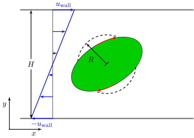
Figure 7: Schematic of the single cell in shear flow. The cell sits in the center of the box and shows an approximately elliptic deformation as well as tank-treading, i. e., a rotation of the membrane around the steady shape in the $x$-$y$-plane

(a)
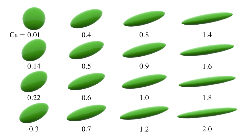
(b)
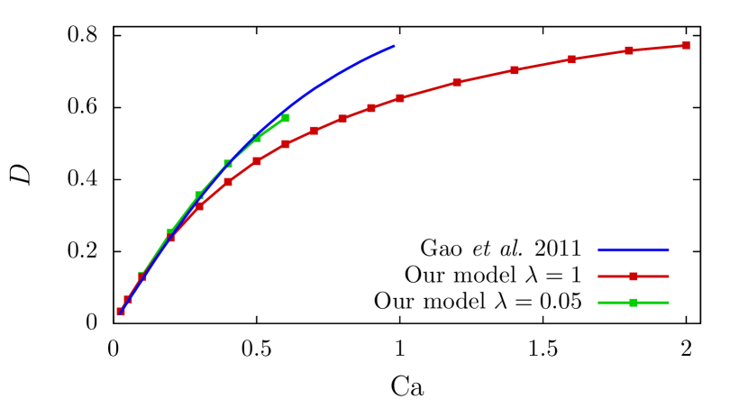
(c)

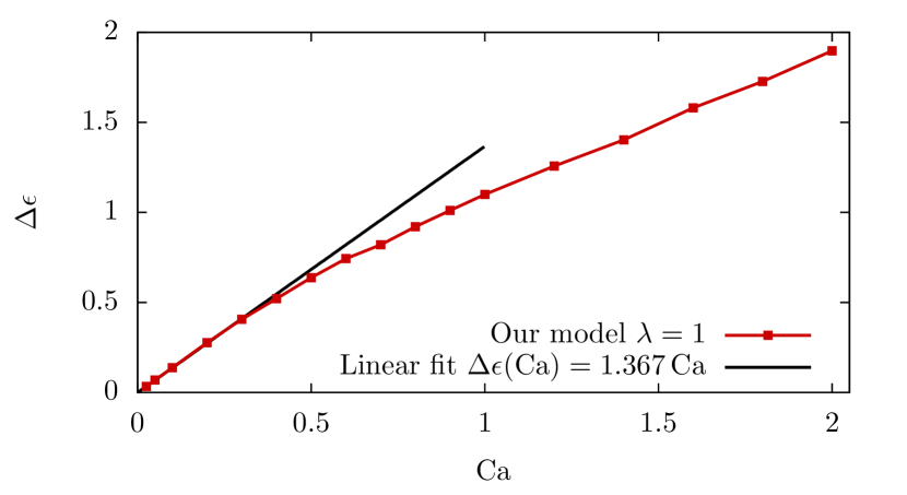
Figure 8: (a) Converged shapes of a single cell in a $10\times 15\times 5$ ($x\times y\times z$) simulation box (in units of the cell radius) with a shear flow in $x$-direction as function of the capillary number $\mathrm{Ca}$. (b) Comparison of our model predictions for a single cell in shear flow to the analytical 3D calculations in figure 7 of Gao et al. [47] in the range of $\mathrm{Ca}\in\left[0.01,2.0\right]$. (c) The relative stretch $\Delta\epsilon$ of our cell model as function of the capillary number $\mathrm{Ca}$. A linear behavior is found for small capillary numbers up to $\mathrm{Ca}=0.3$, while increasing stress is required for larger deformations due to the strain-hardening quality of the neo-Hookean model. Lines are a guide to the eye

6.2 Multiple cell simulations

The second simulation setup, implemented to investigate the multiple particle aspect of our model, consists of $4$ ($8$) cells in a $5\times 8\times 4$ simulation box (in units of the cell radius), corresponding to a volume fraction of $\phi=0.11$ ($\phi=0.22$) occupied by cells. The cells are inserted at random initial positions in the box and the flow parameters are the same as in the first setup (cf. section 6.1).

Figure 9a shows simulation snapshots of the cells in suspensions with volume fraction $\phi=0.11$ and $\phi=0.22$ for $\mathrm{Ca}=0.2$. The Taylor deformation of the suspensions, depicted in figure 9b, is calculated as an average over all cells and over time after an initial transient timespan. We find good agreement when comparing the averaged cell deformation in suspension with Rosti et al. [52], Saadat et al. [53].

(a)
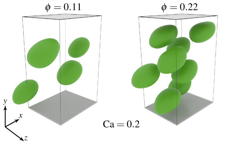
(b)

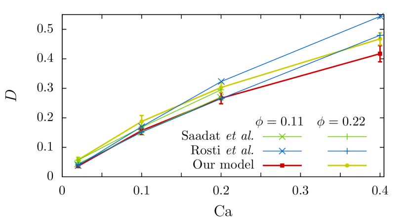
Figure 9: (a) Multiple cells in a $5\times 8\times 4$ ($x\times y\times z$) simulation box (in units of the cell radius) with a confined shear flow in $x$-direction for a capillary number of $\mathrm{Ca}=0.2$ and $4$ cells corresponding to a volume fraction of $\phi=0.11$, and $8$ cells corresponding to $\phi=0.22$. (b) Averaged deformation of multiple cell simulations with $\phi=0.11$ and $\phi=0.22$ in comparison to data from figure 3 of Rosti et al. [52] and figure 13 of Saadat et al. [53]

7 Conclusion

We presented a simple but accurate numerical model for cells and other microscopic particles for the use in computational fluid-particle dynamics simulations.

The elastic behavior of the cells is modeled by applying Mooney–Rivlin strain energy calculations on a uniformly tetrahedralized spherical mesh. We performed a series of FluidFM^®  compression experiments with REF52 cells as an example for cells used in bioprinting processes and found excellent agreement between our numerical model and the measurements if all three parameters of the Mooney–Rivlin model are used. In addition, we showed that the model compares very favorably to force versus deformation data from previous AFM compression experiments on bovine endothelial cells [43] as well as colloidal probe AFM indentation of artificial hydrogel particles [37]. At large deformations, a clear improvement compared to Hertzian contact theory has been observed.

By coupling our model to Lattice Boltzmann fluid calculations via the Immersed-Boundary method, the cell deformation in linear shear flow as function of the capillary number was found in good agreement with analytical calculations by Gao et al. [47] on isolated cells as well as previous simulations of neo-Hookean and viscoelastic solids [52, 53] at various volume fractions.

The presented method together with the precise determination of model parameters by FluidFM^® /AFM experiments may provide an improved set of tools to predict cell deformation - and ultimately cell viability - in strong hydrodynamic flows as occurring, e.g., in bioprinting applications.

See pages - of Supplementary_Information.pdf

References

- Shen et al. [2019] Yigang Shen, Yaxiaer Yalikun, and Yo Tanaka. Recent advances in microfluidic cell sorting systems. Sensors and Actuators B: Chemical, 282:268–281, March 2019. ISSN 09254005. doi: 10.1016/j.snb.2018.11.025.
- Otto et al. [2015] Oliver Otto, Philipp Rosendahl, Alexander Mietke, Stefan Golfier, Christoph Herold, Daniel Klaue, Salvatore Girardo, Stefano Pagliara, Andrew Ekpenyong, Angela Jacobi, Manja Wobus, Nicole Töpfner, Ulrich F Keyser, Jörg Mansfeld, Elisabeth Fischer-Friedrich, and Jochen Guck. Real-time deformability cytometry: On-the-fly cell mechanical phenotyping. Nature Methods, 12(3):199–202, March 2015. ISSN 1548-7091, 1548-7105. doi: 10.1038/nmeth.3281.
- Fregin et al. [2019] Bob Fregin, Fabian Czerwinski, Doreen Biedenweg, Salvatore Girardo, Stefan Gross, Konstanze Aurich, and Oliver Otto. High-throughput single-cell rheology in complex samples by dynamic real-time deformability cytometry. Nature Communications, 10(1):415, December 2019. ISSN 2041-1723. doi: 10.1038/s41467-019-08370-3.
- Kollmannsberger and Fabry [2011] Philip Kollmannsberger and Ben Fabry. Linear and Nonlinear Rheology of Living Cells. Annual Review of Materials Research, 41(1):75–97, August 2011. ISSN 1531-7331, 1545-4118. doi: 10.1146/annurev-matsci-062910-100351.
- Gonzalez-Cruz et al. [2012] Rafael D Gonzalez-Cruz, Vera C Fonseca, and Eric M Darling. Cellular mechanical properties reflect the differentiation potential of adipose-derived mesenchymal stem cells. Proc. Nat. Acad. Sci. (USA), 109(24):E1523–E1529, 2012.
- Huber et al. [2013] F Huber, J Schnau, S Rönicke, P Rauch, K Müller, C Fütterer, and J Käs. Emergent complexity of the cytoskeleton: from single filaments to tissue. Advances in Physics, 62(1):1–112, February 2013.
- Bongiorno et al. [2014] Tom Bongiorno, Jacob Kazlow, Roman Mezencev, Sarah Griffiths, Rene Olivares-Navarrete, John F McDonald, Zvi Schwartz, Barbara D Boyan, Todd C McDevitt, and Todd Sulchek. Mechanical stiffness as an improved single-cell indicator of osteoblastic human mesenchymal stem cell differentiation. J Biomechanics, 47(9):2197–2204, June 2014.
- Fischer-Friedrich et al. [2014] Elisabeth Fischer-Friedrich, Anthony A. Hyman, Frank Jülicher, Daniel J. Müller, and Jonne Helenius. Quantification of surface tension and internal pressure generated by single mitotic cells. Scientific Reports, 4:6213, August 2014. ISSN 2045-2322. doi: 10.1038/srep06213.
- Lange et al. [2015] Janina R Lange, Julian Steinwachs, Thorsten Kolb, Lena A Lautscham, Irina Harder, Graeme Whyte, and Ben Fabry. Microconstriction Arrays for High-Throughput Quantitative Measurements of Cell Mechanical Properties. Biophys. J., 109(1):26–34, July 2015.
- Fischer-Friedrich et al. [2016] Elisabeth Fischer-Friedrich, Yusuke Toyoda, Cedric J. Cattin, Daniel J. Müller, Anthony A. Hyman, and Frank Jülicher. Rheology of the Active Cell Cortex in Mitosis. Biophysical Journal, 111(3):589–600, August 2016. ISSN 00063495. doi: 10.1016/j.bpj.2016.06.008.
- Nyberg et al. [2017] Kendra D Nyberg, Kenneth H Hu, Sara H Kleinman, Damir B Khismatullin, Manish J Butte, and Amy C Rowat. Quantitative Deformability Cytometry: Rapid, Calibrated Measurements of Cell Mechanical Properties. Biophys. J., 113(7):1574–1584, October 2017.
- Lange et al. [2017] Janina R Lange, Claus Metzner, Sebastian Richter, Werner Schneider, Monika Spermann, Thorsten Kolb, Graeme Whyte, and Ben Fabry. Unbiased High-Precision Cell Mechanical Measurements with Microconstrictions. Biophys. J., 112(7):1472–1480, April 2017.
- Kubitschke et al. [2017] H Kubitschke, J Schnauss, K D Nnetu, E Warmt, R Stange, and J Kaes. Actin and microtubule networks contribute differently to cell response for small and large strains. New J. Phys., 19(9):093003–13, September 2017.
- Jaiswal et al. [2017] Devina Jaiswal, Norah Cowley, Zichao Bian, Guoan Zheng, Kevin P. Claffey, and Kazunori Hoshino. Stiffness analysis of 3D spheroids using microtweezers. PLoS One, 12(11):e0188346, 2017.
- Mulla et al. [2019] Yuval Mulla, F C MacKintosh, and Gijsje H Koenderink. Origin of Slow Stress Relaxation in the Cytoskeleton. Phys. Rev. Lett., 122(21):218102, May 2019.
- Snyder et al. [2015] Jessica Snyder, Ae Rin Son, Qudus Hamid, Chengyang Wang, Yigong Lui, and Wei Sun. Mesenchymal stem cell printing and process regulated cell properties. Biofabrication, 7(4):044106, December 2015. ISSN 1758-5090. doi: 10.1088/1758-5090/7/4/044106.
- Blaeser et al. [2015] Andreas Blaeser, Daniela Filipa Duarte Campos, Uta Puster, Walter Richtering, Molly M. Stevens, and Horst Fischer. Controlling Shear Stress in 3D Bioprinting is a Key Factor to Balance Printing Resolution and Stem Cell Integrity. Advanced Healthcare Materials, 5(3):326–333, December 2015. ISSN 2192-2640. doi: 10.1002/adhm.201500677.
- Zhao et al. [2015] Yu Zhao, Yang Li, Shuangshuang Mao, Wei Sun, and Rui Yao. The influence of printing parameters on cell survival rate and printability in microextrusion-based 3D cell printing technology. Biofabrication, 7(4):045002, November 2015. ISSN 1758-5090. doi: 10.1088/1758-5090/7/4/045002.
- Paxton et al. [2017] Naomi Paxton, Willi Smolan, Thomas Böck, Ferry Melchels, Jürgen Groll, and Tomasz Jungst. Proposal to assess printability of bioinks for extrusion-based bioprinting and evaluation of rheological properties governing bioprintability. Biofabrication, 9(4):044107, November 2017. ISSN 1758-5090. doi: 10.1088/1758-5090/aa8dd8.
- Müller et al. [2020] Sebastian J. Müller, Elham Mirzahossein, Emil N. Iftekhar, Christian Bächer, Stefan Schrüfer, Dirk W. Schubert, Ben Fabry, and Stephan Gekle. Flow and hydrodynamic shear stress inside a printing needle during biofabrication. PLOS ONE, 15(7):e0236371, July 2020. ISSN 1932-6203. doi: 10.1371/journal.pone.0236371.
- Khalil and Sun [2007] Saif Khalil and Wei Sun. Biopolymer deposition for freeform fabrication of hydrogel tissue constructs. Materials Science and Engineering: C, 27(3):469–478, April 2007.
- Aguado et al. [2012] Brian A Aguado, Widya Mulyasasmita, James Su, Kyle J Lampe, and Sarah C Heilshorn. Improving Viability of Stem Cells During Syringe Needle Flow Through the Design of Hydrogel Cell Carriers. Tissue Engineering Part A, 18(7-8):806–815, April 2012.
- Tirella et al. [2011] Annalisa Tirella, Federico Vozzi, Giovanni Vozzi, and Arti Ahluwalia. PAM2 (Piston Assisted Microsyringe): A New Rapid Prototyping Technique for Biofabrication of Cell Incorporated Scaffolds. Tissue Engineering Part C: Methods, 17(2):229–237, February 2011.
- Li et al. [2015] Minggan Li, Xiaoyu Tian, Janusz A Kozinski, Xiongbiao Chen, and Dae Kun Hwang. Modeling mechanical cell damage in the bioprinting process employing a conical needle. J. Mech. Med. Biol., 15(05):1550073–15, October 2015.
- Lulevich et al. [2003] V. V. Lulevich, I. L. Radtchenko, G. B. Sukhorukov, and O. I. Vinogradova. Deformation Properties of Nonadhesive Polyelectrolyte Microcapsules Studied with the Atomic Force Microscope. The Journal of Physical Chemistry B, 107(12):2735–2740, March 2003. ISSN 1520-6106, 1520-5207. doi: 10.1021/jp026927y.
- Lulevich et al. [2006] Valentin Lulevich, Tiffany Zink, Huan-Yuan Chen, Fu-Tong Liu, and Gang-yu Liu. Cell Mechanics Using Atomic Force Microscopy-Based Single-Cell Compression. Langmuir, 22(19):8151–8155, September 2006. ISSN 0743-7463, 1520-5827. doi: 10.1021/la060561p.
- Ladjal et al. [2009] Hamid Ladjal, Jean-Luc Hanus, Anand Pillarisetti, Carol Keefer, Antoine Ferreira, and Jaydev P. Desai. Atomic force microscopy-based single-cell indentation: Experimentation and finite element simulation. In 2009 IEEE/RSJ International Conference on Intelligent Robots and Systems, pages 1326–1332, St. Louis, MO, USA, October 2009. IEEE. ISBN 978-1-4244-3803-7. doi: 10.1109/IROS.2009.5354351.
- Kiss [2011] Robert Kiss. Elasticity of Human Embryonic Stem Cells as Determined by Atomic Force Microscopy. Journal of Biomechanical Engineering, 133(10):101009, November 2011. ISSN 0148-0731. doi: 10.1115/1.4005286.
- Hecht et al. [2015] Fabian M Hecht, Johannes Rheinlaender, Nicolas Schierbaum, Wolfgang H Goldmann, Ben Fabry, and Tilman E Schäffer. Imaging viscoelastic properties of live cells by AFM: power-law rheology on the nanoscale. Soft Matter, 11(23):4584–4591, 2015.
- Ghaemi et al. [2016] Ali Ghaemi, Alexandra Philipp, Andreas Bauer, Klaus Last, Andreas Fery, and Stephan Gekle. Mechanical behaviour of micro-capsules and their rupture under compression. Chem. Eng. Sci., 142(C):236–243, March 2016.
- Sancho et al. [2017] Ana Sancho, Ine Vandersmissen, Sander Craps, Aernout Luttun, and Jürgen Groll. A new strategy to measure intercellular adhesion forces in mature cell-cell contacts. Sci. Rep., 7(1):46152–14, April 2017.
- Efremov et al. [2017] Yuri M Efremov, Wen-Horng Wang, Shana D Hardy, Robert L Geahlen, and Arvind Raman. Measuring nanoscale viscoelastic parameters of cells directly from AFM force-displacement curves. Sci. Rep., 7(1):1541–14, May 2017.
- Ladjal et al. [2018] Hamid Ladjal, Jean-Luc Hanus, Anand Pillarisetti, Carol Keefer, Antoine Ferreira, and Jaydev P Desai. Atomic force microscopy-based single-cell indentation: Experimentation and finite element simulation. In 2009 IEEE/RSJ International Conference on Intelligent Robots and Systems (IROS 2009), pages 1326–1332. IEEE, September 2018.
- Chim et al. [2018] Ya Hua Chim, Louise M Mason, Nicola Rath, Michael F Olson, Manlio Tassieri, and Huabing Yin. A one-step procedure to probe the viscoelastic properties of cells by Atomic Force Microscopy. Sci. Rep., 8(1):1–12, September 2018.
- Johnson [2003] Kenneth L. Johnson. Contact Mechanics. Cambridge Univ. Press, Cambridge, 9. print edition, 2003. ISBN 978-0-521-34796-9.
- Dintwa et al. [2008] Edward Dintwa, Engelbert Tijskens, and Herman Ramon. On the accuracy of the Hertz model to describe the normal contact of soft elastic spheres. Granular Matter, 10(3):209–221, March 2008. ISSN 1434-5021, 1434-7636. doi: 10.1007/s10035-007-0078-7.
- Neubauer et al. [2019] Jens W. Neubauer, Nicolas Hauck, Max J. Männel, Maximilian Seuss, Andreas Fery, and Julian Thiele. Mechanoresponsive Hydrogel Particles as a Platform for Three-Dimensional Force Sensing. ACS Applied Materials & Interfaces, 11(29):26307–26313, July 2019. ISSN 1944-8244, 1944-8252. doi: 10.1021/acsami.9b04312.
- Freund [2014] Jonathan B Freund. Numerical Simulation of Flowing Blood Cells. Annu. Rev. Fluid Mech., 46(1):67–95, January 2014.
- Závodszky et al. [2017] Gábor Závodszky, Britt van Rooij, Victor Azizi, and Alfons Hoekstra. Cellular Level In-silico Modeling of Blood Rheology with An Improved Material Model for Red Blood Cells. Front. Physiol., 8:061006–14, August 2017.
- Mauer et al. [2018] Johannes Mauer, Simon Mendez, Luca Lanotte, Franck Nicoud, Manouk Abkarian, Gerhard Gompper, and Dmitry A Fedosov. Flow-Induced Transitions of Red Blood Cell Shapes under Shear. Phys. Rev. Lett., 121(11):118103, September 2018.
- Guckenberger et al. [2018] Achim Guckenberger, Alexander Kihm, Thomas John, Christian Wagner, and Stephan Gekle. Numerical-experimental observation of shape bistability of red blood cells flowing in a microchannel. Soft Matter, 14(11):2032–2043, March 2018.
- Kotsalos et al. [2019] Christos Kotsalos, Jonas Latt, and Bastien Chopard. Bridging the computational gap between mesoscopic and continuum modeling of red blood cells for fully resolved blood flow. J. Comput. Phys., 398:108905, December 2019.
- Caille et al. [2002] Nathalie Caille, Olivier Thoumine, Yanik Tardy, and Jean-Jacques Meister. Contribution of the nucleus to the mechanical properties of endothelial cells. Journal of Biomechanics, 35(2):177–187, February 2002. ISSN 00219290. doi: 10.1016/S0021-9290(01)00201-9.
- Mokbel et al. [2017] M Mokbel, D Mokbel, A Mietke, N Träber, S Girardo, O Otto, J Guck, and S Aland. Numerical Simulation of Real-Time Deformability Cytometry To Extract Cell Mechanical Properties. ACS Biomater. Sci. Eng., 3(11):2962–2973, January 2017.
- Roscoe [1967] R Roscoe. On the rheology of a suspension of viscoelastic spheres in a viscous liquid. J. Fluid Mech., 28(02):273–21, March 1967.
- Gao and Hu [2009] Tong Gao and Howard H. Hu. Deformation of elastic particles in viscous shear flow. Journal of Computational Physics, 228(6):2132–2151, April 2009. ISSN 00219991. doi: 10.1016/j.jcp.2008.11.029.
- Gao et al. [2011] Tong Gao, Howard H Hu, and Pedro Ponte Castañeda. Rheology of a suspension of elastic particles in a viscous shear flow. J. Fluid Mech., 687:209–237, October 2011.
- Gao et al. [2012] Tong Gao, Howard H Hu, and Pedro Ponte Castañeda. Shape Dynamics and Rheology of Soft Elastic Particles in a Shear Flow. Phys. Rev. Lett., 108(5):058302–4, January 2012.
- Lykov et al. [2017] Kirill Lykov, Yasaman Nematbakhsh, Menglin Shang, Chwee Teck Lim, and Igor V Pivkin. Probing eukaryotic cell mechanics via mesoscopic simulations. PLoS Comput Biol, 13(9):e1005726–22, September 2017.
- Villone et al. [2014] M M Villone, M A Hulsen, P D Anderson, and P L Maffettone. Simulations of deformable systems in fluids under shear flow using an arbitrary Lagrangian Eulerian technique. Computers & Fluids, 90(C):88–100, February 2014.
- Villone et al. [2015] M M Villone, G D’Avino, M A Hulsen, and P L Maffettone. Dynamics of prolate spheroidal elastic particles in confined shear flow. Phys. Rev. E, 92(6):062303–12, December 2015.
- Rosti et al. [2018] Marco E. Rosti, Luca Brandt, and Dhrubaditya Mitra. Rheology of suspensions of viscoelastic spheres: Deformability as an effective volume fraction. Physical Review Fluids, 3(1):012301, January 2018. ISSN 2469-990X. doi: 10.1103/PhysRevFluids.3.012301.
- Saadat et al. [2018] Amir Saadat, Christopher J. Guido, Gianluca Iaccarino, and Eric S. G. Shaqfeh. Immersed-finite-element method for deformable particle suspensions in viscous and viscoelastic media. Physical Review E, 98(6):063316, December 2018. ISSN 2470-0045, 2470-0053. doi: 10.1103/PhysRevE.98.063316.
- Alexandrova et al. [2008] Antonina Y. Alexandrova, Katya Arnold, Sébastien Schaub, Jury M. Vasiliev, Jean-Jacques Meister, Alexander D. Bershadsky, and Alexander B. Verkhovsky. Comparative Dynamics of Retrograde Actin Flow and Focal Adhesions: Formation of Nascent Adhesions Triggers Transition from Fast to Slow Flow. PLoS ONE, 3(9):e3234, September 2008. ISSN 1932-6203. doi: 10.1371/journal.pone.0003234.
- Bower [2010] Allan F. Bower. Applied Mechanics of Solids. CRC Press, Boca Raton, 2010. ISBN 978-1-4398-0247-2.
- Mooney [1940] M. Mooney. A Theory of Large Elastic Deformation. Journal of Applied Physics, 11(9):582–592, September 1940. ISSN 0021-8979, 1089-7550. doi: 10.1063/1.1712836.
- Rivlin [1948] R. S. Rivlin. Large Elastic Deformations of Isotropic Materials. I. Fundamental Concepts. Philosophical Transactions of the Royal Society A: Mathematical, Physical and Engineering Sciences, 240(822):459–490, January 1948. ISSN 1364-503X, 1471-2962. doi: 10.1098/rsta.1948.0002.
- Bächer and Gekle [2019] Christian Bächer and Stephan Gekle. Computational modeling of active deformable membranes embedded in three-dimensional flows. Phys. Rev. E, 99(6):062418, June 2019.
- Ramanujan and Pozrikidis [1998] S. Ramanujan and C. Pozrikidis. Deformation of liquid capsules enclosed by elastic membranes in simple shear flow: Large deformations and the effect of fluid viscosities. Journal of Fluid Mechanics, 361:117–143, April 1998. ISSN 0022-1120, 1469-7645. doi: 10.1017/S0022112098008714.
- Clausen and Aidun [2010] Jonathan R. Clausen and Cyrus K. Aidun. Capsule dynamics and rheology in shear flow: Particle pressure and normal stress. Physics of Fluids, 22(12):123302, December 2010. ISSN 1070-6631, 1089-7666. doi: 10.1063/1.3483207.
- Guckenberger et al. [2016] Achim Guckenberger, Marcel P Schraml, Paul G Chen, Marc Leonetti, and Stephan Gekle. On the bending algorithms for soft objects in flows. Comput. Phys. Commun., 207:1–23, October 2016.
- Smith [2009] Michael Smith. ABAQUS/Standard User’s Manual, Version 6.9. Dassault Systèmes Simulia Corp, United States, 2009.
- Limbach et al. [2006] H.J. Limbach, A. Arnold, B.A. Mann, and C. Holm. ESPResSo—an extensible simulation package for research on soft matter systems. Computer Physics Communications, 174(9):704–727, May 2006. ISSN 00104655. doi: 10.1016/j.cpc.2005.10.005.
- Roehm and Arnold [2012] D. Roehm and A. Arnold. Lattice Boltzmann simulations on GPUs with ESPResSo. The European Physical Journal Special Topics, 210(1):89–100, August 2012. ISSN 1951-6355, 1951-6401. doi: 10.1140/epjst/e2012-01639-6.
- Devendran and Peskin [2012] Dharshi Devendran and Charles S Peskin. An immersed boundary energy-based method for incompressible viscoelasticity. J. Comput. Phys., 231(14):4613–4642, May 2012.
- Bächer et al. [2017] Christian Bächer, Lukas Schrack, and Stephan Gekle. Clustering of microscopic particles in constricted blood flow. Phys. Rev. Fluids, 2(1):013102, January 2017.
- Lehmann et al. [2020] Moritz Lehmann, Sebastian Johannes Müller, and Stephan Gekle. Efficient viscosity contrast calculation for blood flow simulations using the lattice Boltzmann method. Int. J. Numer. Meth. Fluids, 103(18):1–15, April 2020.