Highly-Degenerate Photonic Waveguide Structures for Holonomic Computation

Abstract

We investigate an all-out optical setup allowing for generation of non-Abelian geometric phases on its large degenerate eigenspaces. The proposal has the form of an $M$-pod system and can be implemented in terms of integrated photonic waveguide structures. We show that by injecting a larger number of photons into the optical setup, the degeneracy of eigenspaces scales rapidly. After studying the spectral properties of our system for the general case, we show how arbitrary $\mathrm{U}(4)$ transformations can be generated on the dark subspace of an optical tripod filled with two photons. Moreover, a degeneracy in the bright subspaces of the system, absent in any atomic analogue, allows for the generation of universal single-qubit manipulations. Finally, we address the complexity issue of holonomic computation. Particularly, we show how two-qubit and three-qubit states can be implemented on a photonic tripod, where a natural multi-partite structure is inherited from the spatial mode structure of the waveguides.

I Introduction

Quantum computation (QC) and quantum information processing are among the most promising developments in modern physics. Both subjects utilise the fact that the nonclassical nature of certain quantum systems allow for shortcuts in algorithmic evolutions, and in that way speeding up the computation, see e.g. Shor ; Deutsch ; Google . Moreover, quantum information science proposes a number of results about the security of communication channels unmatched by any classical security protocol, e.g. BB84 ; Gottesman . However, the number of astonishing applications seems to be evenly matched by the number of technical challenges one encounters when faced with the task of building an actual quantum computer. Besides the patience and care an experimentalist can provide in preparing a stable and efficient experimental setup, there is an extensive literature on how to make QC robust and fault-tolerant against certain classes of errors Preskill ; QEC .

An important subset of these techniques is referred to as topological quantum information Kitaev1 ; Kitaev2 ; TQC . Roughly speaking, topological methods are based on the idea of error avoidance in contrast to error correction, i.e. protecting the quantum state from a decohering environment or parametric fluctuations, see e.g. Ref. ZanarLloyd2 . In addition to this desirable symmetry-based protection of information, topological QC offers also a deeper insight into a number of geometric and topological notions at an experimentally feasible scale. These notions are not only central to much of modern mathematics, but are prominent features in theories of fundamental interactions as well. Therefore, there has been an increased interest in such topological systems with one focus being on the study and implementation of artificial gauge fields and symmetry groups Zoller1 . Results ranged from implementation of single artificial gauge fields in photonic Szameit2 ; Teuber and atomic systems Spielman to experimental simulation of lattice gauge theories Zoller2 .

In this article, we are mainly concerned with the paradigm of holonomic quantum computation (HQC) HQC ; Pachos99 . HQC is a geometric approach to QC in which the manipulation of quantum information (qubits) is carried out by means of non-Abelian geometric phases following a closed parameter variation (quantum holonomies) Wilzeck . It was shown in Ref. HQC that generically such a computation is universal. The advantage of constructing holonomic quantum gates lies in their parametric robustness so that, in principle, a family of (universal) fault-tolerant quantum gates can be designed in terms of holonomies only Oreshkov ; Oreshkov2 .

Besides its mathematical abstraction, the holonomic route to QC is associated with a series of technical challenges one has to overcome when implementing a (universal) holonomic quantum computer. In particular, HQC demands for the preparation of large degenerate eigenspaces which act as a quantum code Laflamme . To be precise, for a code $\mathcal{C}$ consisting of $k$-qubit code words we need an eigenspace of dimension of at least $2^{k}$. Usually, the degeneracy is ensured by some form of symmetry, i.e. code words in certain subspaces of $\mathcal{C}$ cannot be distinguished energetically. The preparation of such highly symmetric quantum codes becomes a demanding experimental challenge as $k$ increases.

A typical implementation of geometric phases utilises $M$-pod systems Recati that have their origin in atomic physics Bergmann . There, a collection of $M$ ground states is individually coupled to one excited state. Adiabatic parameter variations of the couplings that return to the initial configuration can then implement a (non-Abelian) geometric phase on the $(M-1)$-fold degenerate dark subspace. For instance, a realisation with trapped ions for the case of a tripod ($M=3$) was suggested in Ref. Duan , and another implementation utilised semiconductor macroatoms Rossi . As an extension, there also exist schemes with nonadiabatic parameter variations Sloeqvist ; Abdumalikov ; Kosaka ; Peng . The drawbacks of these systems are that an increase in degeneracy in associated with an increase in the number of ground states, whose implementation can become a challenging task. Furthermore, the listed proposals do not give rise to a proper multi-partite structure by themselves, and many-body interactions have to be considered to construct more intriguing gates.

Here, we present a linear optical implementation of the $M$-pod in the $N$-photon Fock layer giving rise to arbitrarily large degenerate eigenspaces on which HQC could be based. Our proposal can be realised solely in terms of integrated photonic structures such as laser-written silica-based waveguides Szameit . The latter has been proven to be a versatile tool box that combines the proven capabilities of modern quantum optics, like quantum communication Gisin , implementing quantum devices Weinfurter and gates Mataloni ; Benson , or initialising nonclassical states of light Moss ; Tang , with a high degree of interferometric stability. Hence, combining the coherence preserving properties of such structures with the intrinsic robustness of topological QC is a desirable aim.

In fact, there already exist a number of sophisticated works on optical holonomic quantum computation. A first theoretical proposal for an optical holonomic quantum computer goes back to Ref. PachosOpt , where a quantum holonomy generated from a nonlinear Kerr Hamiltonian was designed by driving squeezing and displacement in a suitable manner such that the desired gate can be obtained. In comparison to this early idea, our proposal is solely based on linear evanescent coupling of the waveguides and thus, nonlinearities have to be added to extend optical HQC to a universal scheme Shen , e.g. measurement-based KLM ; Scheel . In a more recent work on optical HQC, spin-orbit coupling of polarised light in asymmetric microcavities is utilised to generate a geometric phase Schmidt , whereas the emergence of a non-Abelian Berry phase was observed when injecting coherent states of light into topologically guided modes Chamon . In Ref. Teuber , an artificial non-Abelian gauge potential was designed by driving an adiabatic path in the dark subspace of an optical tripod. However, the current implementations are all limited to only doubly degenerate subspaces and thus only enable the study of $\mathrm{U}(2)$ holonomies.

In our present work, we overcome the limitations of current HQC schemes by increasing the number of photons involved in the dynamical evolution. As a result, the degeneracy of the system is easily increased. We further propose that, from the large number of degenerate eigenspaces, one will eventually find a subspace on which the spatial mode structure of the waveguide modes can be used to label logical qubits, even though the entire eigenspace might not possess a proper multi-partite structure. Therefore, our proposal overcomes another problem frequently occurring in HQC since its inception Pachos99 .

We finally note that, as a linear optical scheme, our setup is closely related to standard approaches of linear optical quantum computation based on large networks of beam splitters Reck-Zeil ; O'Brien ; Laing . However, in constrast to such schemes, where each beam splitter (and phase shifter) has to be adjusted individually with potential fluctuations, holonomic approaches generate the desired evolution in one collective fault-tolerant dynamic which is especially true if larger degeneracies are achieved.

The structure of the article is as follows. In Sec. II, we present the quantum optical $M$-pod which allows for the implementation of arbitrarily large degenerate subspaces and study its spectral properties. Section III is dedicated to a review of the basic theory of HQC, to the extent as it is relevant to our study of the photonic setup. In Sec. IV, a detailed discussion of an optical tripod, represented in the two-photon Fock layer, illustrates how arbitrary holonomic $\mathrm{U}(4)$ transformations can be realised within the degenerate eigenspaces of the waveguide arrangement. The complexity question regarding the construction of logical quantum information (code words) is addressed in Sec. V, where we show how to define the code words on the total Hilbert space of the system and act with holonomies from different eigenspaces onto a code $\mathcal{C}$. More precisely, we show how one can use the optical tripod to prepare two-qubit and three-qubit states. Finally, Sec. VI contains a summary of the article as well as some concluding remarks. In Appendix A we give an explicit parameter-dependent representation of the dark and bright states in the two-photon Fock layer. App. B contains details of a diagonalisation of the $M$-pod system in terms of bosonic field operators, showing how the eigenstates distribute over the different eigenspaces. In App. C we design simple parameter variations that induce a number of useful quantum gates via a non-Abelian geometric phase.

II Degeneracy in photonic waveguides

Let us consider the optical setup depicted in Fig. 1, in which $M+1$ waveguides are arranged in the form of an $M$-pod. The Hamiltonian of the system reads

$$H=\sum_{i=1}^{M}\left(\kappa_{i}a_{i}a^{\dagger}_{M+1}+\kappa_{i}^{*}a_{i}^{\dagger}a_{M+1}\right)$$ (1)

(we set $\hbar=1$ throughout this work), where $a_{j}^{\dagger}$ ($a_{j}$) is the bosonic creation (annihilation) operator for the $j$-th waveguide mode ($j=1,\dots,M+1$) and $\kappa_{i}$ is the coupling strength between the $i$-th outer waveguide with the central waveguide.

Figure 1: Schematic front view of an $M$-pod waveguide arrangement subject to the Hamiltonian in Eq. (1). The $i$-th outer waveguide ($i=1,\dots,M$) interacts solely with the central one via the coupling $\kappa_{i}$.

Next, we restrict the Hamiltonian (1) to act solely on the $N$-photon Fock layer

$$\mathcal{F}_{N}=\biggr{\{}\ket{n_{1},\dots n_{M+1}}\,\biggr{|}\,\sum_{j=1}^{M+1}n_{j}=N\biggr{\}}.$$ (2)

Represented in the basis $\mathcal{F}_{N}$, the Hamiltonian $H$ from Eq. (1) defines an operator on the reduced Hilbert space $\mathcal{H}=\mathrm{Span}(\mathcal{F}_{N})$ having dimension $p=(N+M)!/(N!M!)$, which is the number of possibilities to distribute $N$ identical photons on $(M+1)$ labelled waveguides.

Choosing an index system for the $p$ Fock states, one can calculate a matrix representation $\bm{H}=(H_{ij})_{i,j=1}^{p}$ in $\mathcal{F}_{N}$. By diagonalisation of this matrix one finds a decomposition of the Hilbert space $\mathcal{H}$ into orthogonal eigenspaces, viz.

$$\mathcal{H}=\mathcal{H}_{\mathcal{D}}\oplus\mathcal{H}_{\mathcal{B}_{+}}\oplus\mathcal{H}_{\mathcal{B}_{-}}\oplus\dots\oplus\mathcal{H}_{\mathcal{B}_{+}}^{(N)}\oplus\mathcal{H}_{\mathcal{B}_{-}}^{(N)},$$ (3)

where $\mathcal{H}_{\mathcal{D}}$ is its dark subspace (eigenspace with eigenvalue zero), and $\mathcal{H}_{\mathcal{B}_{\pm}}^{(n)}$ is the eigenspace corresponding to the energy $\pm n\varepsilon=\pm n\sqrt{|\kappa_{1}|^{2}+\dots+|\kappa_{M}|^{2}}$ ($n=1,\dots,N$).

The degeneracy of these subspaces depends on the number of waveguides and photons and can explicitly be calculated, see App. B. For the dimension $d(N,M)$ of $\mathcal{H}_{\mathcal{D}}$ we find

$$d(N,M)=\begin{cases}\sum_{n=1}^{N/2}{{2n+M-2}\choose{2n}},&\text{if $N$ even,}\\ \sum_{n=0}^{(N-1)/2}{{2n+1+M-2}\choose{2n+1}},&\text{if $N$ odd,}\end{cases}$$ (4)

and for all subsequent subspaces $\mathcal{H}_{\mathcal{B}_{\pm}},\mathcal{H}_{\mathcal{B}_{\pm}}^{(2)},\dots$ one finds $d(N-1,M),d(N-2,M),\dots$, respectively. In Fig. 2, the resulting spectral structure is schematically shown for selected values of $N$ and $M$. Clearly, the addition of more photons drastically increases the available dimensions of subspaces on which one can perform HQC protocols.

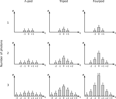
Figure 2: Spectrum of an $M$-pod system filled with $N$ photons. The number of eigenstates ($\#$) is depicted over the energy (in multiples of $\varepsilon$) for $M,N\in\{1,2,3\}$. Additional waveguides lead to an increase in the degree of degeneracy of the eigenenergies. The degeneracy of the lowest levels (magnitudewise) increases the most, while the two highest (magnitudewise) energy levels are nondegenerate. In comparison, increasing the number of photons in the system, not only increases degeneracy but gives rise to two additional nondegenerate eigenenergies. The profile of the bar diagram becomes steeper as $M$ increases.

In comparison, adding another state to an atomic $M$-pod system (which might be a challenging task) yields only one additional dark state. By utilising the tools of waveguide quantum optics one is thus able to increase the degeneracy in two ways. First, one can engineer an additional waveguide with coupling solely to the central waveguide (see Fig. 1). This will increase the dimension of each eigenspace depending on the number of photons participating in the optical experiment. From Fig. 1, one observes that increasing the number of waveguide arms in the $M$-pod will fail when $M$ becomes large, because placing too many waveguides around the central one will ultimately result in a coupling of the outer waveguides with each other, thus breaking the structure of the $M$-pod. This problem can be avoided by following the alternative route by sending a higher number of photons into the $M$-pod.

In the following, after reviewing some basic theory, we will illustrate an interesting application, in which the prepared degenerate eigenspaces are utilised to allow for the manipulation of (geometric) quantum information. It turns out that our photonic setup allows, in principle, to implement rotations between the degenerate eigenstates such that the whole unitary group $\mathrm{U}(m)$ for arbitrary $m\in\mathbb{N}$ can be spanned in a purely geometric way.

III Computation with holonomies

For a working HQC procedure one seeks a computational scheme in which a geometric property, the holonomy, plays the role of the unitary gate. For the following investigation we make the usual assumption that the Hamiltonian $H$ of a quantum system can be expressed in terms of control fields $\bm{\lambda}=\{\lambda_{\mu}\}_{\mu=1}^{D}$ (couplings) which serve as local coordinates on a $D$-dimensional parameter space $\mathcal{M}$ (control manifold). If one is able to drive the control field configuration through a (piecewise) smooth path $\gamma:[0,T]\rightarrow\mathcal{M}$, we have $H[\bm{\lambda}(t)]=H_{\gamma(t)}$ and the quantum system evolves according to $U(T)=\bm{\hat{\mathrm{T}}}\mathrm{e}^{-\mathrm{i}\int_{0}^{T}H_{\gamma(t)}\mathrm{d}t}$ ($\bm{\hat{\mathrm{T}}}$ denotes time ordering). In this context, HQC is based on the idea that generating a sufficient, finite set of paths $\{\gamma_{i}\}$ induces a sequence of corresponding gates $\{U_{i}\}$ implementing the whole quantum information network HQC .

Here, we are not interested in arbitrary paths but in those that represent loops in $\mathcal{M}$, that is, $\gamma(T)=\gamma(0)=\bm{\lambda}_{0}$. Let us further suppose that the Hamiltonian defines an iso-degenerate (no level-crossing) family of Hermitian operators with $R$ different eigenvalues. Then one has the $\bm{\lambda}$-dependent spectral decomposition $H(\bm{\lambda})=\sum_{j=1}^{R}\varepsilon_{j}(\bm{\lambda})\Pi_{j}(\bm{\lambda})$. Here $\Pi_{j}(\bm{\lambda})$ is the projector onto the $m_{j}$-fold degenerate eigenspace $\mathcal{H}_{j}(\bm{\lambda})=\mathrm{Span}(\{\ket{\psi_{j,a}(\bm{\lambda})}\}^{m_{j}}_{a=1})$, corresponding to the energy $\varepsilon_{j}(\bm{\lambda})$.

We restrict ourselves to adiabatic loops, i.e. the change of the control fields happens slow enough such that transitions to states of different eigenenergies are prohibited Fock . From the adiabatic assumption it follows that any initial preparation $\ket{\psi(0)}=\ket{\psi_{\mathrm{in}}}\in\mathcal{H}_{j}$ is mapped, after a time period $T$, onto a final state $U(T)\ket{\psi_{\mathrm{in}}}$ lying also in $\mathcal{H}_{j}$. Hence, the time evolution consists of a sum of unitary evolutions within each degenerate subspace $\mathcal{H}_{j}$. Explicitly, we have HQC

$$U(T) = \oplus_{j=1}^{R}\mathrm{e}^{\mathrm{i}\omega_{j}(T)}W^{(j)}(\gamma),$$ (5)

$$W^{(j)}(\gamma) = \bm{\hat{\mathrm{P}}}\mathrm{exp}\oint_{\gamma}A_{j}\in\mathrm{U}(m_{j}),$$ (6)

where the first exponential, with $\omega_{j}(T)=\int_{0}^{T}\varepsilon_{j}(\bm{\lambda}(t))\mathrm{d}t$, is the dynamical phase while the second term $W^{(j)}(\gamma)$ is a quantum holonomy determined by the path-ordered exponentiation of the matrix-valued phase factor $\oint A_{j}$. Here, $A_{j}=\Pi_{j}(\bm{\lambda})\mathrm{d}\Pi_{j}(\bm{\lambda})$ is a non-Abelian gauge potential often referred to as the adiabatic connection (local connection one-form). Its (anti-Hermitian) components read

$$\left(A_{j,\mu}\right)_{ab}=\bra{\psi_{j,a}(\bm{\lambda})}\partial_{\mu}\ket{\psi_{j,b}(\bm{\lambda})},$$ (7)

such that $A_{j}=\sum_{\mu=1}^{D}A_{j,\mu}\mathrm{d}\lambda_{\mu}$ ($\partial_{\mu}=\partial/\partial\lambda_{\mu}$).

The set of transformations $W^{(j)}(\{\gamma_{i}\})$ generated from a set of loops $\{\gamma_{i}\}$ at an initial point $\bm{\lambda}_{0}$ forms a subgroup of the unitary group $\mathrm{U}(m_{j})$ that is known as the holonomy group $\mathrm{Hol}(A_{j})$. A lower bound for the dimension of $\mathrm{Hol}(A_{j})$ is given by the number of linear independent components of the local curvature two-form $F_{j}=\sum_{\mu<\nu}^{D}F_{j,\mu\nu}\mathrm{d}\lambda_{\mu}\wedge\mathrm{d}\lambda_{\nu}$ ($\wedge$ denotes the antisymmetrised tensor product) Recati ; Nakahara . Its antisymmetric components can be computed from

$$F_{j,\mu\nu}=\partial_{\mu}A_{j,\nu}-\partial_{\nu}A_{j,\mu}+[A_{j,\mu},A_{j,\nu}],$$ (8)

where $[A_{j,\mu},A_{j,\nu}]$ denotes the commutator. The curvature is a measure for the nontrivial topology on $\mathcal{M}$, which manifests itself in the richness of holonomic transformations on the subspace $\mathcal{H}_{j}$. If the connection $A_{j}$ is irreducible, then the holonomy group coincides with the whole $\mathrm{U}(m_{j})$. In Ref. HQC it was proven that two generic loops in $\mathcal{M}$ are sufficient to generate a dense subset of the unitary group, that is, any element in $\mathrm{U}(m_{j})$ can be approximated to arbitrary precision by implementing a finite product sequence of these loops. Clearly, if $\mathcal{H}_{j}$ can be viewed as a multi-qubit code, then the irreducibility of the connection is equivalent to the notion of computational universality for $m_{j}\geq 4$ Divi ; Lloyd .

IV Two-photon tripod holonomies

In this section, we illustrate the previous general scheme on the example of a photonic tripod represented in the two-photon Fock layer. For $M=3$ and $N=2$, the relevant Fock states are

$$\begin{split}\mathcal{F}_{2}=\{&\ket{1100},\ket{0110},\ket{1010},\ket{0011},\ket{0101},\\ &\ket{1001},\ket{2000},\ket{0200},\ket{0020},\ket{0002}\}.\\ \end{split}$$ (9)

In this Fock layer, the Hamiltonian from Eq. (1) gives rise to a four-dimensional dark subspace $\mathcal{H}_{\mathcal{D}}$, spanned by dark states $\{\ket{D_{a}(\bm{\kappa})}\}_{a=1}^{4}$ (details in App. A). In the following, we show how to generate arbitrary $\mathrm{U}(4)$ transformations on $\mathcal{H}_{\mathcal{D}}$. To ensure this, we will enact a pair of noncommuting holonomies $W_{1}^{(\mathcal{D})}$ and $W_{2}^{(\mathcal{D})}$. Let us choose local coordinates $\kappa_{i}=r_{i}\mathrm{e}^{\mathrm{i}\theta_{i}}$, with $r_{i}\geq 0$ and $\theta_{i}\in[0,2\pi)$ that parametrise the $\bm{\kappa}$-space $\mathcal{M}$. In the notation of Sec. III this means $\lambda_{\mu}\in\{r_{i},\theta_{i}\}_{i=1}^{3}$. For the generation of nontrivial holonomies, a certain richness of the control space $\mathcal{M}$ has to be provided. It turns out that, in our case, one needs at least three real coordinates (this holds even for all $N$ and $M$) to ensure a nonvanishing curvature (8), that can give rise to a quantum holonomy.

For the first transformation we set $\kappa_{1}=0$, $\kappa_{2}=r_{2}\mathrm{e}^{\mathrm{i}\theta_{2}}$, and $\kappa_{3}=r_{3}$. Note, that there are indeed many existing schemes to realise (effective) complex coupling strengths, see e.g. Refs. Esslinger ; Cages . Next, we derive the dark states with respect to the parametrisation $\{r_{2},\theta_{2},r_{3}\}$ of $\mathcal{M}$ as shown in Eq. (7). Due to the complex coupling one obtains connection coefficients with nonvanishing diagonal elements, that is

$$A_{\theta_{2}}=\begin{pmatrix}0&0&0&0\\ 0&\frac{\mathrm{i}r_{3}^{2}}{r_{2}^{2}+r_{3}^{2}}&0&0\\ 0&0&\frac{2\mathrm{i}r_{3}^{2}}{r_{2}^{2}+r_{3}^{2}}&0\\ 0&0&0&\frac{\mathrm{i}r_{2}^{2}}{r_{2}^{2}+r_{3}^{2}}\\ \end{pmatrix}$$ (10)

(all remaining components vanish), written in the basis of dark states (view App. A for details) at an initial point $\bm{\kappa}_{0}$ in $\mathcal{M}$.

A nonvanishing connection enables us to generate purely geometric rotations within the dark subspace. More precisely, traversing an arbitrary loop $\gamma$ in $\mathcal{M}$ results in the holonomy

$$W_{1}^{(\mathcal{D})}(\gamma)=\mathrm{exp}\left(\oint_{\gamma}A_{\theta_{2}}\mathrm{d}\theta_{2}\right)$$ (11)

where path ordering becomes obsolete, due to the fact that there is only one relevant component. The evaluation of the matrix exponential in Eq. (11) becomes quite simple due to the diagonal form of $A_{\theta_{2}}$.

For generating the second transformation, we activate all three couplings $\kappa_{1}=r_{1}$, $\kappa_{2}=r_{2}$, and $\kappa_{3}=r_{3}$. A quite similar calculation as before reveals that the connection coefficients are given by $A_{r_{1}}=-\mathrm{i}\sqrt{2}\zeta_{213}(\bm{r})\Sigma$ and $A_{r_{2}}=\mathrm{i}\sqrt{2}\zeta_{123}(\bm{r})\Sigma$, while $A_{r_{3}}$ vanishes. Here we made use of the definitions

$$\Sigma=\begin{pmatrix}0&1&0&0\\ -1&0&1&0\\ 0&-1&0&0\\ 0&0&0&0\\ \end{pmatrix},\quad\zeta_{ijk}(\bm{r})=\frac{r_{i}r_{k}}{(r_{i}^{2}+r_{j}^{2})r},$$ (12)

where $r=\sqrt{r_{1}^{2}+r_{2}^{2}+r_{3}^{2}}$. Due to commuting connection coefficients, path ordering can be neglected again. Hence, the corresponding matrix exponential can still be evaluated explicitly so that the holonomy reads

$$W_{2}^{(\mathcal{D})}(\gamma)=\begin{pmatrix}\cos^{2}(\phi_{0})&\sqrt{2}\sin(\phi_{0})\cos(\phi_{0})&\sin^{2}(\phi_{0})&0\\ -\sqrt{2}\sin(\phi_{0})\cos(\phi_{0})&\cos(2\phi_{0})&\sqrt{2}\sin(\phi_{0})\cos(\phi_{0})&0\\ \sin^{2}(\phi_{0})&-\sqrt{2}\sin(\phi_{0})\cos(\phi_{0})&\cos^{2}(\phi_{0})&0\\ 0&0&0&1\\ \end{pmatrix},$$ (13)

with

$$\phi_{0}(\gamma)=\oint_{\gamma}\zeta_{123}(\bm{r})\mathrm{d}r_{2}-\zeta_{213}(\bm{r})\mathrm{d}r_{1}$$ (14)

being a geometric phase factor. It turns out that the holonomies (11) and (13) do not commute for generic loops in $\mathcal{M}$. Thus, it is shown how, in principle, any $\mathrm{U}(4)$ transformation on $\mathcal{H}_{\mathcal{D}}$ can be approximated arbitrarily well in terms of holonomies only. More generally, our photonic setup provides us, indeed, with the possibility to implement qudit states (i.e. $\mathcal{H}_{\mathcal{D}}\cong\mathbb{C}^{m}$) on which arbitrary $\mathrm{U}(m)$ holonomies act.

Further, note that in comparison to atomic physics, where a fivepod is necessary to obtain holonomic $\mathrm{U}(4)$ transformations, in photonic waveguide structures one only needs to design a tripod system. The optical setup has another advantage over the usual atomic scheme as we will illustrate in the following. In the representation of $\mathcal{F}_{2}$, the photonic structure gives also rise to a twofold degeneracy in the bright states $\ket{B_{1}^{(\pm)}(\bm{\kappa})},\ket{B_{2}^{(\pm)}(\bm{\kappa})}$, which is absent in atomic $M$-pod systems. Their respective eigenenergies are $\pm\sqrt{|\kappa_{1}|^{2}+|\kappa_{2}|^{2}+|\kappa_{3}|^{2}}$. It is straightforward to show that one can generate arbitrary $\mathrm{U}(2)$ manipulations on each of the eigenspaces $\mathcal{H}_{\mathcal{B}_{+}}$ and $\mathcal{H}_{\mathcal{B}_{-}}$. To be precise, let $\ket{B_{1}^{(\pm)}},\ket{B_{2}^{(\pm)}}$ be the bright states spanning $\mathcal{H}_{\mathcal{B}_{+}}$ and $\mathcal{H}_{\mathcal{B}_{-}}$, respectively. In the case of three real coupling parameters, the corresponding connections reads

$$A_{\pm,r_{1}}=-\mathrm{i}\zeta_{312}(\bm{r})\sigma_{y}^{(\pm)},\quad A_{\pm,r_{3}}=\mathrm{i}\zeta_{132}(\bm{r})\sigma_{y}^{(\pm)},$$ (15)

while $A_{\pm,r_{2}}=0$. Here, we defined

$$\begin{split}\sigma_{y}^{(\pm)}&=\mathrm{i}\ket{B_{2}^{(\pm)}(\bm{\kappa}_{0})}\bra{B_{1}^{(\pm)}(\bm{\kappa}_{0})}-\mathrm{i}\ket{B_{1}^{(\pm)}(\bm{\kappa}_{0})}\bra{B_{2}^{(\pm)}(\bm{\kappa}_{0})},\end{split}$$ (16)

where we have chosen $\bm{\kappa}_{0}=(0,0,\kappa)$ ($\kappa=\mathrm{const.}$) as the initial point at which the holonomy is generated. The general parameter-dependent form of the bright states is contained in App. A. Fortunately, path ordering can be omitted, because all $A_{r_{i}}$ commute with one another, that means we found an Abelian substructure of the system. With the connection at hand, we are able to design the adiabatic holonomy

$$W_{1}^{(\pm)}(\gamma)=\mathrm{e}^{\mathrm{i}\phi_{1}(\gamma)\sigma_{y}^{(\pm)}}=\begin{pmatrix}\cos\phi_{1}&\sin\phi_{1}\\ -\sin\phi_{1}&\cos\phi_{1}\\ \end{pmatrix}$$ (17)

with the geometric phase

$$\begin{split}\phi_{1}(\gamma)&=\oint_{\gamma}\zeta_{132}(\bm{r})\mathrm{d}r_{3}-\zeta_{312}(\bm{r})\mathrm{d}r_{1},\end{split}$$ (18)

and the matrix in Eq. (17) being written in the basis

$$\begin{split}\ket{B_{1}^{(\pm)}(\bm{\kappa}_{0})}&=\frac{1}{\sqrt{2}}\left(\ket{1010}\pm\ket{1001}\right),\\ \ket{B_{2}^{(\pm)}(\bm{\kappa}_{0})}&=\frac{1}{\sqrt{2}}\left(\ket{0110}\pm\ket{0101}\right).\\ \end{split}$$ (19)

A second holonomy can be obtained in a similar way. To ensure that the transformations do not commute, a complex coupling between one of the outer waveguides and the central one has to be implemented. Here, we set $\kappa_{1}=r_{1}\mathrm{e}^{\mathrm{i}\theta_{1}}$. Moreover, let $\kappa_{2}=0$, so that we are only concerned with loops $\gamma$ described by coordinates $\{r_{1},\theta_{1},r_{3}\}$ on $\mathcal{M}$. At the point $\bm{\kappa}_{0}$, the holonomic unitary for this parametrisation takes the form $W_{2}^{(\pm)}=\mathrm{e}^{\mathrm{i}\phi_{2}}\ket{B_{1}^{(\pm)}}\bra{B_{1}^{(\pm)}}+\mathrm{e}^{\mathrm{i}\tilde{\phi}_{2}}\ket{B_{2}^{(\pm)}}\bra{B_{2}^{(\pm)}}$, depending on the geometric phase factors

$$\phi_{2}(\gamma)=\oint_{\gamma}\frac{r_{1}^{2}+2r_{3}^{2}}{2(r_{1}^{2}+r_{3}^{2})}\mathrm{d}\theta_{1},\quad\tilde{\phi}_{2}(\gamma)=\oint_{\gamma}\frac{r_{1}^{2}}{2(r_{1}^{2}+r_{3}^{2})}\mathrm{d}\theta_{1},$$ (20)

with $\gamma$ being another loop in $\mathcal{M}$. From here on it is easy to check that the transformations $W_{1}^{(\pm)}$ and $W_{2}^{(\pm)}$ do not commute, and thus the existence of a universal set of single-qubit gates on $\mathcal{H}_{\mathcal{B}_{\pm}}$ is verified.

Note that, unlike in the case of the dark states, the bright states accumulate not only a geometric phase but a dynamical phase as well. The latter one reads $\mathrm{e}^{\pm\mathrm{i}\int_{0}^{T}\sqrt{|\kappa_{1}|^{2}+|\kappa_{2}|^{2}+|\kappa_{3}|^{2}}\mathrm{d}t}$. We should stress that such dynamical contributions do not possess the robustness and fault-tolerance of a purely holonomic quantum gate. However, it was proven in Ref. Oreshkov3 that robust QC can be done efficiently on subsystems (different eigenspaces) of the total Hilbert space in a fully holonomic fashion. In Ref. Oreshkov it was further shown that such a computation can be made, in principle, completely fault-tolerant, by providing additional syndrome and gauge qubits.

V Remarks on the computational complexity of subsystems

As our theoretical proposal provides eigenspaces with arbitrarily large degrees of degeneracy, the question arises as to how efficient QC can be done on these spaces. We start by recalling that an $M$-pod filled with $N$ photons is described by $(N+M)!/(N!M!)$ orthogonal Fock states distributed over $2N+1$ separate eigenspaces. However, we have to note that generically an eigenspace $\mathcal{H}_{j}$, from the decomposition (3), does not need to support a proper multi-partite structure. By that we mean that there is no guarantee that one can decompose $\mathcal{H}_{j}$ into a product of single-qubit Hilbert spaces in any physically relevant way Zanardi . More formally speaking, the algebra of observables (here the $C^{*}$-algebra of bosonic creation and annihilation operators) does not inherit a tensor-product structure solely restricted to $\mathcal{H}_{j}$ Zanardi ; ZanarLloyd . This problem occurs frequently in the paradigm of HQC and has to be overcome to ensure a consistent labelling of logical qubits Pachos99 .

One possible solution to this difficulty might be to use the natural multi-partite structure induced by the Hamiltonian (1). The total Hilbert space over which this observable acts can be decomposed with respect to the spatial modes of each waveguide, i.e. $\mathcal{H}=\mathrm{Span}(\{\otimes_{j}\ket{k}_{j}\}_{k=0}^{n_{j}})$ (recall that $\sum_{j}n_{j}=N$). From this point of view, we are able to implement a maximal number of $M+1$ qudits, with their dimension corresponding to the number of photons in the waveguide system. As simple this solution might seem at first sight, it leads to a rather subtle issue. In the scenario under investigation the generated holonomies may not act as a proper quantum gate solely within one of the eigenspaces, but rather on a logical quantum code $\mathcal{C}\subseteq\mathcal{H}$. A series of holonomies in different eigenspaces might then be needed to produce the desired transformation on the level of Fock states. Nevertheless, because one can generate any transformation on each of the respective eigenspaces, it may be well possible, if the eigenspaces are large enough, to generate any linear optical computation within a subspace of $\mathcal{H}$, which has a natural multi-partite structure inherited from the spatial-mode structure of the waveguides.

V.1 Implementation of Two-Qubit States

Let us clarify the above statements by a generic example. In the following, we will show how the two-photon tripod from Sec. IV serves as a sufficient setup for the implementation of two-qubit states. For that, recall that the first order bright subspaces $\mathcal{H}_{\mathcal{B}_{\pm}}$ at the point $\bm{\kappa}_{0}=(0,0,\kappa)$ are spanned by the states (19). Logical qubits are then defined with respect to the spatial mode structure of the waveguide network, viz. $\ket{0}_{\mathrm{L}}=\ket{1}_{1,3}\otimes\ket{0}_{2,4}$ and $\ket{1}_{\mathrm{L}}=\ket{0}_{1,3}\otimes\ket{1}_{2,4}$. With this definition at hand, the two-qubit states

$$\begin{split}\ket{00}_{\mathrm{L}}&=\ket{1010},\qquad\ket{10}_{\mathrm{L}}=\ket{0110},\\ \ket{01}_{\mathrm{L}}&=\ket{1001},\qquad\ket{11}_{\mathrm{L}}=\ket{0101},\\ \end{split}$$ (21)

lie completely within the quantum code $\mathcal{C}=\mathcal{H}_{\mathcal{B}_{+}}\oplus\mathcal{H}_{\mathcal{B}_{-}}$. The labelling in Eq. (21) preserves the underlying bipartite structure of the waveguides. Hence, we have a physical realisation of two-qubit states. After a (holonomic) quantum algorithm transformed an initial preparation $\ket{\psi_{\mathrm{in}}}$ into the desired answer $\ket{\psi_{\mathrm{out}}}$ of a computational problem, the output state can be measured by a set of photo detectors at the output facets of the waveguides. Note that the bright states decompose into product states with respect to the bi-partition of the waveguides (21),

$$\begin{split}\ket{B_{1}^{(\pm)}(\bm{\kappa}_{0})}&=\ket{0}_{\mathrm{L}}\otimes\ket{\pm},\\ \ket{B_{2}^{(\pm)}(\bm{\kappa}_{0})}&=\ket{1}_{\mathrm{L}}\otimes\ket{\pm},\\ \end{split}$$ (22)

where $\ket{\pm}=(\ket{0}_{\mathrm{L}}\pm\ket{1}_{\mathrm{L}})/\sqrt{2}$ denotes the diagonal basis. With this explicit representation one can investigate how arbitrary holonomies act on the code $\mathcal{C}$ in terms of the qubits (21).

For the purpose of illustration, let us focus on a benchmark holonomy. In Sec. IV we explained that the connections over $\mathcal{H}_{\mathcal{B}_{+}}$ and $\mathcal{H}_{\mathcal{B}_{-}}$ are irreducible. It thus follows that, by adiabatically varying the Hamiltonian (1) along a suitable loop in $\mathcal{M}$, we are able to apply the gate [cf. Eq. (5)]

$$U(\omega_{\pm},\gamma)=\mathrm{e}^{\mathrm{i}\omega_{+}}W^{(+)}(\gamma)\oplus\mathrm{e}^{\mathrm{i}\omega_{-}}W^{(-)}(\gamma)$$ (23)

to the qubits (21), where $W^{(+)}$ and $W^{(-)}$ are now arbitrary holonomies acting within each subspace on the states (22). Recall that $\omega_{\pm}$ denote the integrals over the eigenenergies of $\mathcal{H}_{\mathcal{B}_{+}},\mathcal{H}_{\mathcal{B}_{-}}$, respectively. In particular, it holds that $\omega_{\pm}=\pm\omega$ with $\omega>0$. For concreteness, let us consider the unitaries from Eq. (17). Then, a composite holonomy $U_{1}(\omega,\phi)$ [cf. Eq. (23)] acts on the computational basis (21) according to the truth table

$$\begin{split}\ket{00}_{\mathrm{L}}&\mapsto\ket{\phi_{1}}\otimes\ket{\omega},\qquad\ket{10}_{\mathrm{L}}\mapsto\ket{\overline{\phi}_{1}}\otimes\ket{\omega},\\ \ket{01}_{\mathrm{L}}&\mapsto\ket{\phi_{1}}\otimes\ket{\overline{\omega}},\qquad\ket{11}_{\mathrm{L}}\mapsto\ket{\overline{\phi}_{1}}\otimes\ket{\overline{\omega}},\\ \end{split}$$ (24)

where we introduced the $\phi_{1}$-dependent states

$$\begin{split}\ket{\phi_{1}}&=\cos\phi_{1}\ket{0}_{\mathrm{L}}-\sin\phi_{1}\ket{1}_{\mathrm{L}},\\ \ket{\overline{\phi}_{1}}&=\cos\phi_{1}\ket{1}_{\mathrm{L}}+\sin\phi_{1}\ket{0}_{\mathrm{L}},\\ \end{split}$$ (25)

together with the $\omega$-dependent states

$$\begin{split}\ket{\omega}&=\cos\omega\ket{0}_{\mathrm{L}}+\mathrm{i}\sin\omega\ket{1}_{\mathrm{L}},\\ \ket{\overline{\omega}}&=\cos\omega\ket{1}_{\mathrm{L}}+\mathrm{i}\sin\omega\ket{0}_{\mathrm{L}}.\\ \end{split}$$ (26)

The latter describe a dynamical superposition of the vacuum and the one-photon Fock state localized in the third or fourth waveguide, while the former are of purely geometric origin and distribute over the first two modes. By designing a plaquette $\square$ in $\mathcal{M}$ such that $\phi_{1}(\square)=-\pi/4$ (details in App. C) the logical qubits obey the transformation $XH\otimes\Omega(\omega)$, where a Hadamard gate $H=\ket{0}_{\mathrm{L}}\bra{+}+\ket{1}_{\mathrm{L}}\bra{-}$ acts on the first qubit (first and second waveguide) followed by the bit-flip gate $X=\ket{0}_{\mathrm{L}}\bra{1}_{\mathrm{L}}+\ket{1}_{\mathrm{L}}\bra{0}_{\mathrm{L}}$, while simultaneously the gate $\Omega(\omega)=\ket{\omega}\bra{0}_{\mathrm{L}}+\ket{\overline{\omega}}\bra{1}_{\mathrm{L}}$ acts on the second qubit (third and fourth waveguide). The gate $\Omega$ parametrises a great circle traversing through the poles ($\ket{0}_{\mathrm{L}}$ and $\ket{1}_{\mathrm{L}}$) of the Bloch sphere (cf. Fig. 3). In comparison, the action on the first qubit has no inherent dynamical contribution and is therefore robust towards experimental imperfections that undermine the plaquette $\square$.

Figure 3: Bloch sphere representation of the states $\ket{\phi_{1}}$ and $\ket{\omega}$. Manipulating the geometric phase factor $\phi_{1}$ results in a motion along the red great circle. In comparison, a change in the dynamical part $\omega$ moves the state along the blue great circle. By combining both transformations any state on the the Bloch sphere can be reached.

Designing another loop $\gamma$ such that $\phi_{1}(\gamma)=\pi/2$ (cf. App. C) creates the quantum circuit $\mathrm{i}Y\otimes\Omega(\omega)$, with $Y=\mathrm{i}(\ket{1}_{\mathrm{L}}\bra{0}_{\mathrm{L}}-\ket{0}_{\mathrm{L}}\bra{1}_{\mathrm{L}})$ being the Pauli-$Y$ gate. If the experimenter is able to change the rate with which the path is traversed, this will not influence the quantum holonomic gate (as long as adiabaticity holds) but can realise a desired transformation on the second qubit in terms of a dynamical gate.

A different quantum gate $U_{2}(\omega,\gamma)$ is obtained by inserting the holonomy $W_{2}^{(\pm)}(\gamma)$ (recall Sec. IV) into Eq. (23). This gate obeys the truth table

$$\begin{split}\ket{00}_{\mathrm{L}}&\mapsto\mathrm{e}^{\mathrm{i}\phi_{2}}\ket{0}_{\mathrm{L}}\otimes\ket{\omega},\quad\ket{10}_{\mathrm{L}}\mapsto\mathrm{e}^{\mathrm{i}\tilde{\phi}_{2}}\ket{1}_{\mathrm{L}}\otimes\ket{\omega},\\ \ket{01}_{\mathrm{L}}&\mapsto\mathrm{e}^{\mathrm{i}\phi_{2}}\ket{0}_{\mathrm{L}}\otimes\ket{\overline{\omega}},\quad\ket{11}_{\mathrm{L}}\mapsto\mathrm{e}^{\mathrm{i}\tilde{\phi}_{2}}\ket{1}_{\mathrm{L}}\otimes\ket{\overline{\omega}},\\ \end{split}$$ (27)

with the path-dependent geometric phases $\phi_{2}$ and $\tilde{\phi}_{2}$ from Eq. (20). The unitary (27) corresponds to a product of single qubit gates, that is, $U_{2}=P\otimes\Omega$, with $P=\mathrm{e}^{\mathrm{i}\phi_{2}}\ket{0}_{\mathrm{L}}\bra{0}_{\mathrm{L}}+\mathrm{e}^{\mathrm{i}\tilde{\phi}_{2}}\ket{1}_{\mathrm{L}}\bra{1}_{\mathrm{L}}$ being a phase gate. The quantum gates $U_{1}$ and $U_{2}$ in general do not commute. From Fig. 3 we can conclude that the gates we provided form a dense subset of the unitary group $\mathrm{U}(2)\otimes\mathrm{U}(2)\subset\mathrm{U}(4)$ and thus, we are, in principle, able to approximate any of its elements to arbitrary precision.

V.2 Implementation of Three-Qubit States

For the preparation of larger code words than two-qubit states we need to enlarge the number of states on which to perform holonomic computation, that is, we need to prepare larger degenerate eigenspaces. Because encoded information lies in a proper subspace $\mathcal{C}$ of the total Hilbert space $\mathcal{H}$, the quantum code is most generally a subspace reaching over several eigenspaces of $\mathcal{H}$. Let us illustrate this point by constructing three-qubit states, i.e. we have $\mathcal{C}\cong(\mathbb{C}^{2})^{\otimes^{3}}\cong\mathbb{C}^{8}$. Therefore, one has to inject another photon into the optical tripod from Sec. IV, that is, we study the tripod in the three-photon Fock layer. Analogously to Sec. IV, one can show that, in principle, any unitary transformation can be carried out over the first-order bright subspaces $\mathcal{H}_{\mathcal{B}_{+}}$ and $\mathcal{H}_{\mathcal{B}_{-}}$ in terms of quantum holonomies. Both eigenspaces are fourfold degenerate and are spanned as $\mathcal{H}_{\mathcal{B}_{\pm}}=\mathrm{Span}(\{\ket{B_{a}^{(\pm)}}\}_{a=1}^{4})$. In addition, we take the nondegenerate third-order bright subspaces $\mathcal{H}_{\mathcal{B}_{+}}^{(3)}$ and $\mathcal{H}_{\mathcal{B}_{-}}^{(3)}$ into account. Subsequently, the eight-dimensional quantum code $\mathcal{C}$ will be a proper subspace of the ten-dimensional Hilbert space $\mathcal{H}_{\mathcal{B}_{+}}\oplus\mathcal{H}_{\mathcal{B}_{-}}\oplus\mathcal{H}_{\mathcal{B}_{+}}^{(3)}\oplus\mathcal{H}_{\mathcal{B}_{-}}^{(3)}$ that preserves the tri-partite (spatial-mode) structure of the three outer waveguides.

We found a consistent labelling to be

$$\begin{split}\ket{000}_{\mathrm{L}}=\ket{0003},&\quad\ket{100}_{\mathrm{L}}=\ket{3000},\\ \ket{010}_{\mathrm{L}}=\ket{0201},&\quad\ket{001}_{\mathrm{L}}=\ket{0021},\\ \ket{110}_{\mathrm{L}}=\ket{1200},&\quad\ket{101}_{\mathrm{L}}=\ket{1020},\\ \ket{011}_{\mathrm{L}}=\ket{0111},&\quad\ket{111}_{\mathrm{L}}=\ket{1110}.\\ \end{split}$$ (28)

In Eq. (28), the logical zero corresponds to the vacuum state, and the logical one is encoded when at least one photon impinges onto the detector in the respective waveguide. The qubits (Fock states) in Eq. (28) can be expressed solely through bright states in $\mathcal{H}_{\mathcal{B}_{+}}\oplus\mathcal{H}_{\mathcal{B}_{-}}\oplus\mathcal{H}_{\mathcal{B}_{+}}^{(3)}\oplus\mathcal{H}_{\mathcal{B}_{-}}^{(3)}$, hence at the point $\bm{\kappa}_{0}=(\kappa,0,0)$ we have

$$\begin{split}\ket{000}_{\mathrm{L}}&=\frac{1}{2\sqrt{2}}\left(\ket{B^{(+3)}(\bm{\kappa}_{0})}+\ket{B^{(-3)}(\bm{\kappa}_{0})}\right)+\frac{\sqrt{3}}{2\sqrt{2}}\left(\ket{B_{1}^{(+)}(\bm{\kappa}_{0})}+\ket{B_{1}^{(-)}(\bm{\kappa}_{0})}\right),\\ \ket{100}_{\mathrm{L}}&=\frac{1}{2\sqrt{2}}\left(\ket{B^{(+3)}(\bm{\kappa}_{0})}-\ket{B^{(-3)}(\bm{\kappa}_{0})}\right)-\frac{\sqrt{3}}{2\sqrt{2}}\left(\ket{B_{1}^{(+)}(\bm{\kappa}_{0})}-\ket{B_{1}^{(-)}(\bm{\kappa}_{0})}\right),\\ \end{split}$$ (29)

$$\begin{split}\ket{010}_{\mathrm{L}}&=\frac{1}{\sqrt{2}}\left(\ket{B_{4}^{(+)}(\bm{\kappa}_{0})}+\ket{B_{4}^{(-)}(\bm{\kappa}_{0})}\right),\qquad\ket{001}_{\mathrm{L}}=\frac{1}{\sqrt{2}}\left(\ket{B_{2}^{(+)}(\bm{\kappa}_{0})}+\ket{B_{2}^{(-)}(\bm{\kappa}_{0})}\right),\\ \ket{110}_{\mathrm{L}}&=\frac{1}{\sqrt{2}}\left(\ket{B_{4}^{(+)}(\bm{\kappa}_{0})}-\ket{B_{4}^{(-)}(\bm{\kappa}_{0})}\right),\qquad\ket{101}_{\mathrm{L}}=\frac{1}{\sqrt{2}}\left(\ket{B_{2}^{(+)}(\bm{\kappa}_{0})}-\ket{B_{2}^{(-)}(\bm{\kappa}_{0})}\right),\\ \ket{011}_{\mathrm{L}}&=\frac{1}{\sqrt{2}}\left(\ket{B_{3}^{(+)}(\bm{\kappa}_{0})}+\ket{B_{3}^{(-)}(\bm{\kappa}_{0})}\right),\qquad\ket{111}_{\mathrm{L}}=\frac{1}{\sqrt{2}}\left(\ket{B_{3}^{(+)}(\bm{\kappa}_{0})}-\ket{B_{3}^{(-)}(\bm{\kappa}_{0})}\right).\\ \end{split}$$ (30)

Note that there are two remaining states $\ket{1002}$ and $\ket{2001}$ in $\mathcal{H}_{\mathcal{B}_{+}}\oplus\mathcal{H}_{\mathcal{B}_{-}}\oplus\mathcal{H}_{\mathcal{B}_{+}}^{(3)}\oplus\mathcal{H}_{\mathcal{B}_{-}}^{(3)}$ that can, in principle, introduce an over-labelling of logical states. When the experimenter is just observing if a detector, placed at the output facet of the first waveguide, did or did not click, the states can be mistaken as the qubit $\ket{100}_{\mathrm{L}}$. To avoid this undesirable phenomenom, we do not choose arbitrary holonomies on $\mathcal{H}_{\mathcal{B}_{+}}\oplus\mathcal{H}_{\mathcal{B}_{-}}\oplus\mathcal{H}_{\mathcal{B}_{+}}^{(3)}\oplus\mathcal{H}_{\mathcal{B}_{-}}^{(3)}$, but those which map the code $\mathcal{C}$, i.e. the qubits from Eq. (28), onto itself.

VI Conclusion

In this article, we have presented a theoretical proposal for the implementation of arbitrary $\mathrm{U}(m)$ transformations, to satisfactory precisions, by holonomic means. Our photonic setup consisted solely of directional couplers which were arranged as an $M$-pod system. We found that, upon injecting additional photons into the waveguide system, the degeneracy of eigenspaces scaled drastically. In comparison to atomic $M$-pod systems, where a linear increase in degeneracy can only be observed in the dark subspace, our setup can produce a nonlinear increase in the degeneracy of each eigenspace.

For the special scenario of the two-photon optical tripod, the associated connections revealed that arbitrary geometric transformations can be designed on the eigenspaces of the system. This was explicitly shown for the group $\mathrm{U}(4)$. We have shown how one can use the spatial mode structure of the waveguides to define a consistent labelling of logical qubits. This was explicitly demonstrated for the case of two-qubit states. Our scheme provides the utility of implementing robust quantum gates in terms of a composite holonomy generated over the twofold degenerate bright subspaces of the system. Moreover, we showed how three-qubit states can be labelled on the optical tripod by injecting a third photon, thus illustrating that our photonic scheme is scalable in terms of providing additional qubits.

Our article paves the way for an experimental study of large holonomy groups and the transformation behaviour of bosonic Fock states under their action. It shows that the problem of having no natural multi-partite structure on the computational eigenspaces can be overcome by considering subspaces so large, that a natural multi-partite quantum code can be realised within them.

Appendix A Dark States and Bright States for the Two-Photon Tripod

In the following, explicit formulas for the dark states and first order bright states of the two-photon tripod are given. From these states, one can directly calculate the respective connections according to Eq. (7). Recall the first parametrisation used for the dark subspace holonomy, with $\kappa_{1}=0$, $\kappa_{2}=r_{2}\mathrm{e}^{\mathrm{i}\theta_{2}}$, and $\kappa_{3}=r_{3}$ with $r_{i}\geq 0$ and $\theta_{i}\in[0,2\pi)$. Under this parametrisation the (orthogonalised) dark states take the form

$$\begin{split}\ket{D_{1}}&=\ket{2000},\\ \ket{D_{2}}&=\frac{1}{\rho_{23}}\left(r_{2}\ket{1010}-r_{3}\mathrm{e}^{\mathrm{i}\theta_{2}}\ket{1100}\right),\\ \ket{D_{3}}&=\frac{1}{\rho_{23}^{2}}\left(r_{3}^{2}\mathrm{e}^{2\mathrm{i}\theta_{2}}\ket{0200}-\sqrt{2}r_{2}r_{3}\mathrm{e}^{\mathrm{i}\theta_{2}}\ket{0110}+r_{2}^{2}\ket{0020}\right),\\ \ket{D_{4}}&=\frac{1}{\sqrt{2}\rho_{23}^{2}}\left(r_{2}^{2}\mathrm{e}^{2\mathrm{i}\theta_{2}}\ket{0200}+r_{3}^{2}\ket{0020}\right)+\frac{r_{2}r_{3}}{\rho_{23}^{2}}\mathrm{e}^{\mathrm{i}\theta_{2}}\ket{0110}-\frac{1}{\sqrt{2}}\ket{0002},\\ \end{split}$$ (31)

with $\rho_{ij}=\sqrt{r_{i}^{2}+r_{j}^{2}}$. Next, for the real-valued coordinates $\kappa_{1}=r_{1}$, $\kappa_{2}=r_{2}$, and $\kappa_{3}=r_{3}$, the dark states read

$$\begin{split}\ket{D_{1}}&=\frac{1}{\rho_{12}^{2}}\left(r_{2}^{2}\ket{2000}-\sqrt{2}r_{1}r_{2}\ket{1100}+r_{1}^{2}\ket{0200}\right),\\ \ket{D_{2}}&=\frac{\sqrt{2}r_{1}r_{2}r_{3}}{\rho_{12}^{2}r}\left(\ket{0200}-\ket{2000}\right)+\frac{1}{r}\left(r_{2}\ket{1010}-r_{1}\ket{0110}\right)+\frac{(r_{1}^{2}-r_{2}^{2})r_{3}}{\rho_{12}^{2}r}\ket{1100},\\ \ket{D_{3}}&=\frac{r_{3}^{2}}{\rho_{12}^{2}r^{2}}\left(r_{1}^{2}\ket{2000}+r_{2}^{2}\ket{0200}\right)+\frac{\sqrt{2}r_{3}}{r^{2}}\left(\frac{r_{1}r_{2}r_{3}}{\rho_{12}^{2}}\ket{1100}-r_{1}\ket{1010}-r_{2}\ket{0110}\right)+\frac{\rho_{12}^{2}}{r^{2}}\ket{0020},\\ \ket{D_{4}}&=\frac{1}{\sqrt{2}r^{2}}\left(r_{1}^{2}\ket{2000}+r_{2}^{2}\ket{0200}+r_{3}^{2}\ket{0020}\right)+\frac{1}{r^{2}}\left(r_{1}r_{2}\ket{1100}+r_{1}r_{3}\ket{1010}+r_{2}r_{3}\ket{0110}\right)-\frac{1}{\sqrt{2}}\ket{0002},\\ \end{split}$$ (32)

where we defined $r=\sqrt{r_{1}^{2}+r_{2}^{2}+r_{3}^{2}}$. From these two sets of states the adiabatic connection and subsequently the holonomies (11) and (13) were computed.

We now turn to the first-order bright states, which were used in Subsection V.1 to define logical two-qubit states. To obtain the geometric phase factors in Eq. (20) we chose local coordinates $\kappa_{1}=r_{1}\mathrm{e}^{\mathrm{i}\theta_{1}}$, $\kappa_{2}=0$, and $\kappa_{3}=r_{3}$. The first order bright states in $\mathcal{H}_{\mathcal{B}_{+}}$ and $\mathcal{H}_{\mathcal{B}_{-}}$ are found to be

$$\begin{split}\ket{B_{1}^{(\pm)}}&=\frac{r_{1}r_{3}}{\rho_{13}^{2}}\left(\mathrm{e}^{2\mathrm{i}\theta_{1}}\ket{2000}-\ket{0020}\right)\pm\frac{1}{\sqrt{2}\rho_{13}}\left(r_{3}\mathrm{e}^{\mathrm{i}\theta_{1}}\ket{1001}-r_{1}\ket{0011}\right)+\frac{r_{3}^{2}-r_{1}^{2}}{\sqrt{2}\rho_{13}^{2}}\mathrm{e}^{\mathrm{i}\theta_{1}}\ket{1010},\\ \ket{B_{2}^{(\pm)}}&=\frac{1}{\sqrt{2}\rho_{13}}\left(r_{3}\ket{0110}+r_{1}\mathrm{e}^{\mathrm{i}\theta_{1}}\ket{1100}\right)\pm\frac{1}{\sqrt{2}}\ket{0101}.\\ \end{split}$$ (33)

For the second transformation the couplings were $\kappa_{1}=r_{1}$, $\kappa_{2}=r_{2}$, and $\kappa_{3}=r_{3}$. The bright states for this case are

$$\begin{split}\ket{B_{1}^{(\pm)}}&=\frac{r_{1}r_{3}}{r\rho_{13}}\left(\ket{2000}-\ket{0020}\right)+\frac{r_{2}}{\sqrt{2}r\rho_{13}}\left(r_{3}\ket{1100}-r_{1}\ket{0110}\right)\pm\frac{1}{\sqrt{2}\rho_{13}}\left(r_{3}\ket{1001}-r_{1}\ket{0011}\right)+\frac{r_{3}^{2}-r_{1}^{2}}{\sqrt{2}r\rho_{13}}\ket{1010},\\ \ket{B_{2}^{(\pm)}}&=\frac{\rho_{13}}{r}\left(\frac{r_{2}}{r}\ket{0200}\pm\frac{1}{\sqrt{2}}\ket{0101}\right)-\frac{r_{2}}{\rho_{13}r^{2}}\left(r_{1}^{2}\ket{2000}+\sqrt{2}r_{1}r_{3}\ket{1010}+r_{3}^{2}\ket{0020}\right)\\ &\hskip 14.22636pt\mp\frac{r_{2}}{\sqrt{2}r\rho_{13}}\left(r_{1}\ket{1001}+r_{3}\ket{0011}\right)+\frac{r_{1}^{2}-r_{2}^{2}+r_{3}^{2}}{\sqrt{2}\rho_{13}r^{2}}\left(r_{1}\ket{1100}+r_{3}\ket{0110}\right).\\ \end{split}$$ (34)

From the above states we were able to compute the holonomy (17). Moreover, one can easily check that in the limit $\bm{\kappa}\rightarrow\bm{\kappa}_{0}=(0,0,\kappa)$ the basis (19) is reproduced.

Appendix B Dimension of Subspaces

The dimensions of the subspaces in an $M$-pod with $N$ photons injected can be determined as follows. In case of only one photon or excitation the same result applies as in atomic physics Dalibard , i.e. in an $M$-pod term scheme there is one negative bright state, one positive and $M-1$ dark states. This means that the Hamiltonian in Eq. (1) can be rewritten with new bosonic mode operators $b_{-},d_{1},\dots,d_{M-1},b_{+}$ as

$$H=-\varepsilon b^{\dagger}_{-}b_{-}+\varepsilon b^{\dagger}_{+}b_{+},$$ (35)

where only the bright modes occur because of the zero eigenvalue of the dark modes. The advantage of this representation of $H$ is that we can now simply turn to a Fock state notation when considering the case of $N$ photons. The eigenstates of the Hamiltonian can then be given by the number of photons $n_{-}$ in the negative bright mode, the number of photons $n_{+}$ in the positive bright mode, and $n_{\mathcal{D}}$ as the number of photons in the $M-1$ dark modes. The eigenvalue equation of these Fock states is

$$H|n_{-},n_{\mathcal{D}},n_{+}\rangle=\varepsilon(n_{+}-n_{-})|n_{-},n_{\mathcal{D}},n_{+}\rangle$$ (36)

with $n_{-}+n_{\mathcal{D}}+n_{+}=N$.

Counting the number of dark states in the $N$ photon case then amounts to counting the number of possibilities to distribute $N$ photons so that the eigenvalue $\varepsilon(n_{+}-n_{-})$ becomes zero. Clearly, this is the case when either all $N$ photons are distributed over the $M-1$ dark modes, or when an equal number of photons are in the positive and negative bright modes with the rest in the dark modes. For example, there are ${{N+M-2}\choose{2n}}$ ways of distributing all photons over the dark modes. Next, one can have one photon in each positive and negative bright mode, thus ${{N-2+M-2}\choose{N-2}}$ ways remain to distribute the rest of the photons over the dark modes. This continues until all photons are equally distributed over the positive and negative bright modes. However, there are two distinct cases, $N$ odd or even, for which one finds two formulas for the total number of dark states, i.e.

$$d(N,M)=\begin{cases}\sum_{n=1}^{N/2}{{2n+M-2}\choose{2n}},&\text{if $N$ even,}\\ \sum_{n=0}^{(N-1)/2}{{2n+1+M-2}\choose{2n+1}},&\text{if $N$ odd.}\end{cases}$$ (37)

When counting the number of bright states with energy $\pm k\varepsilon$, one first has to put $k$ photons in either the negative or positive bright mode, and then distribute the rest as if to create a dark state. Thus, for bright states with energy $\pm k\varepsilon$ there are $d(N-k,M)$ possibilities.

Appendix C Computation of Non-Abelian Geometric Phases

Here, we shall give an explicit way to obtain the geometric phases $\phi_{1}(\gamma)$ that implement the desired quantum gates in Subsection V.1. We recall from Sec. IV that the holonomies in Eq. (17), which act on the bright subspaces $\mathcal{H}_{\mathcal{B}_{+}}$ and $\mathcal{H}_{\mathcal{B}_{-}}$ respectively, are completely determined by the scalar $\phi_{1}(\gamma)$ from Eq. (18). The line integral on which the phase factor depends can be replaced by a surface integral using Stokes’ Theorem Nakahara

$$\oint_{\gamma}A_{\pm}=\int_{\mathcal{S}}F_{\pm}=\mathrm{i}\phi_{1}(\mathcal{S})\sigma_{y}^{(\pm)},$$ (38)

where $\mathcal{S}$ is the area in the $D$-dimensional control space $\mathcal{M}$, which is enclosed by the loop $\gamma$. Given the connection coefficients from Eq. (15), one readily obtains the curvature (8) with respect to $\mathcal{H}_{\mathcal{B}_{\pm}}$, namely

$$\begin{split}F_{\pm,r_{1}r_{2}}&=\mathrm{i}r_{3}/r^{3}\sigma_{y}^{(\pm)},\\ F_{\pm,r_{1}r_{3}}&=-\mathrm{i}r_{2}/r^{3}\sigma_{y}^{(\pm)},\\ F_{\pm,r_{2}r_{3}}&=\mathrm{i}r_{1}/r^{3}\sigma_{y}^{(\pm)}.\\ \end{split}$$ (39)

Note that in Eq. (39) all components of the curvature commute so that not only is path ordering obsolete, but the commutator in Eq. (8) vanishes.

As the precise form of the generating loop does not matter, one might as well design a simple plaquette

$$\square(\alpha,\beta)=\left\{\bm{r}\in\mathbb{R}^{3}\,\bigr{|}\,r_{1}\in[0,\alpha],\,r_{2}\in[0,\beta],\,r_{3}=\kappa\right\},$$ (40)

that is, restricting oneself to the $(r_{1},r_{2})$-plane at $r_{3}=\kappa=\mathrm{const}$. In this context, $\alpha$ and $\beta$ determine the area enclosed by $\square$, such that the desired geometric phase factor can be attained. Under the constraints given by the plaquette (40), the integration over an oriented surface reduces to $\iint_{\square}F_{\pm,r_{1}r_{2}}\mathrm{d}r_{1}\mathrm{d}r_{2}$. Hence, the relevant phase factor becomes

$$\phi_{1}(\square)=\int_{0}^{\beta}\int_{0}^{\alpha}\frac{\kappa\mathrm{d}r_{1}\mathrm{d}r_{2}}{\sqrt{r_{1}^{2}+r_{2}^{2}+\kappa^{2}}^{3}}.$$ (41)

Fortunately, the integration can be performed analytically so that we obtain

$$\phi_{1}(\alpha,\beta)=\mathrm{arctan}\left(\frac{\alpha\beta}{\kappa\sqrt{\alpha^{2}+\beta^{2}+\kappa^{2}}}\right).$$ (42)

By appropriately choosing $\alpha>\kappa$ and $\beta=\kappa\sqrt{(\alpha^{2}+\kappa^{2})/(\alpha^{2}-\kappa^{2})}$, the phase factor (42) can be set to $\phi_{1}(\alpha,\beta)=-\pi/4$, which implements the gate $XH$ on the first qubit (cf. Subsection. V.1).

Next, we show how to realise the holonomic gate $\mathrm{i}Y$ also discussed in Subsection V.1. In this case, it turns out to be suitable to parametrise the $(\kappa_{1},\kappa_{2})$-plane as $\kappa_{1}=\kappa\sin\varphi\cos\vartheta$ and $\kappa_{2}=\kappa\sin\varphi\sin\vartheta$, with $\varphi,\vartheta\in[0,2\pi)$, which can involve negative couplings for certain values of $\varphi$ and $\vartheta$. The surface integral transforms accordingly to

$$\phi_{1}(\mathcal{S})=\iint_{\mathcal{S}}\frac{\kappa}{\sqrt{\kappa_{1}^{2}+\kappa_{2}^{2}+\kappa^{2}}^{3}}\frac{\partial(\kappa_{1},\kappa_{2})}{\partial(\varphi,\vartheta)}\mathrm{d}\varphi\mathrm{d}\vartheta,$$ (43)

where the Jacobian is

$$\frac{\partial(\kappa_{1},\kappa_{2})}{\partial(\varphi,\vartheta)}=\kappa^{2}\sin\varphi\cos\varphi>0$$ (44)

for $\varphi\in(0,\pi/2)$. Direct integration of (43) gives

$$\begin{split}\phi_{1}(\mathcal{S})&=\int_{\vartheta_{0}}^{\vartheta_{1}}\int_{\varphi_{0}}^{\varphi_{1}}\frac{\sin\varphi\cos\varphi}{\sqrt{1+\sin^{2}\varphi}}\mathrm{d}\varphi\mathrm{d}\vartheta,\\ &=\left(\sqrt{\sin^{2}\varphi_{1}+1}-\sqrt{\sin^{2}\varphi_{0}+1}\right)\left[\vartheta_{1}-\vartheta_{0}\right].\\ \end{split}$$ (45)

In order to implement the desired gate, we shall design the geometric phase (43) as $\phi_{1}(\mathcal{S})=\pi/2$ for which we can choose $\varphi_{0}=0$, $\varphi_{1}=\pi/2$, and $\vartheta_{1}-\vartheta_{0}=\pi/(2\sqrt{2}-2)$.

References

- (1) P. Shor, in Proceedings 35th Annual Symposium on Fundamentals of Computer Science (IEEE Press, Los Alamitos, CA, 1994).
- (2) D. Deutsch and R. Jozsa, Proc. Roy. Soc. Lond. A 439, 553 (1992).
- (3) F. Arute, K. Arya, R. Babbush, et al., Nature 574, 505 (2019).
- (4) C. H. Bennett and G. Brassard, Proc. IEEE Int. Conf. Comp. 175, 8 (1984).
- (5) D. Gottesman and H.-K. Lo, IEEE Trans. Inf. Theo. 49, 457 (2003).
- (6) D. A. Lidar and T. A. Brun, Quantum Error Correction (Cambridge University Press, Cambridge, 2013).
- (7) J. Preskill, CALT-68-2150, QUIC-97-034 (1999).
- (8) M. Fredman, A. Y. Kitaev, M. Larsen, and Z. Wang, Bull. Amer. Math. Soc. 40, 31 (2003).
- (9) A. Y. Kitaev, Ann. of Phys. 303, 2 (2003).
- (10) V. T. Lahtinen and J. K. Pachos, SciPost Phys. 3, 021 (2017).
- (11) P. Zanardi and Seth Lloyd, Phys. Rev. Lett. 90, 067902 (2003)
- (12) M. C. Bauls et al., arXiv preprint, arXiv:1911.00003 [quant-ph] (2019).
- (13) Y. Lumer et al., Nat. Photonics 13, 339 (2019).
- (14) M. Kremer, L. Teuber, A. Szameit, and S. Scheel, Phys. Rev. Res. 1, 033117 (2019).
- (15) V. Galitski, G. Juzeliūnas, and Ian B. Spielman, Phys. Today 72, 38 (2019).
- (16) E. A. Martinez et al., Nature (London) 534, 516 (2016).
- (17) P. Zanardi and M. Rasetti, Phys. Lett. A 264, 94 (1999).
- (18) J. Pachos, P. Zanardi, and M. Rasetti, Phys. Rev. A 61, 010305(R) (1999).
- (19) F. Wilczek and A. Zee, Phys. Rev. Lett. 52, 2111 (1984).
- (20) O. Oreshkov, T. A. Brun, and D. A. Lidar, Phys. Rev. Lett. 102, 070502 (2009).
- (21) O. Oreshkov, T. A. Brun, and D. A. Lidar, Phys. Rev. A 80, 022325 (2009).
- (22) D. Kribs, R. Laflamme, and D. Poulin, Phys. Rev. Lett. 94, 180501 (2005).
- (23) A. Recati, T. Calarco, and P. Zanardi, J. I. Cirac, and P. Zoller, Phys. Rev. A 66, 032309 (2002).
- (24) R. G. Unanyan, B. W. Shore, and K. Bergmann, Phys. Rev. A 59, 2910 (1998).
- (25) L. M. Duan, J. Cirac, and P. Zoller, Science 292, 1695 (2001).
- (26) E. Biolatti, R. C. Iotti, P. Zanardi, and F. Rossi, Phys. Rev. Lett. 85, 5647 (2000).
- (27) E. Sjöqvist, D M Tong , L M. Andersson, Björn Hessmo, M. Johansson, and K. Singh, New J. Phys. 14, 103035 (2012).
- (28) A. A. Abdumalikov, Jr., J. M. Fink, K. Juliusson, M. Pechal, S. Berger, A. Wallraff, and S. Filipp, Nature (London) 496, 482 (2013).
- (29) K. Nagata, K. Kuramitani, Yuhei Sekiguchi, and H. Kosaka, Nat. Commun. 9, 3227 (2018).
- (30) Z. Zhu, T. Chen, X. Yang, J. Bian, Z.-Y. Xue, and X. Peng, Phys. Rev. App. 12, 024024 (2019).
- (31) A. Szameit and S. Nolte, J. Phys. B: At. Mol. Opt. Phys. 43, 163001 (2010).
- (32) S. Tanzilli, W. Tittel, H. De Riedmatten, H. Zbinden, P. Baldi, M. De Micheli, D. B. Ostrowsky, and N. Gisin, Eur. Phys. J. D 18, 155 (2002).
- (33) C. Schuck, G. Huber, C. Kurtsiefer, and H. Weinfurter, Phys. Rev. Lett 96, 190501 (2006).
- (34) G. Kewes et al, Sci. Rep. 6, 28877 (2016).
- (35) A. Crespi, R. Ramponi, R. Osellame, L. Sansoni, I. Bongioanni, F. Sciarrino, G. Vallone, and P. Mataloni, Nat. Commun. 2, 566 (2011).
- (36) X. Guo, C.-l. Zou, C. Schuck, H. Jung, R. Cheng, and H. X. Tang, Light Sci Appl. 6, e16249 (2017).
- (37) L. Caspani, C. Xiong, B. J. Eggleton, D. Bajoni, M. Liscidini, M. Galli, R. Morandotti, and D. J. Moss, Light: Sci. & Apps. 6, e17100 (2017).
- (38) J. Pachos and S. Chountasis, Phys. Rev. A 62, 052318 (2000).
- (39) Y. R. Shen, The Principles of Nonlinear Optics (Wiley, New York, 1984).
- (40) E. Knill, R. Laflamme, and G. J. Milburn, Nature (London) 409, 46 (2001).
- (41) S. Scheel, K. Nemoto, W. J. Munro, and P. L. Knight, Phys. Rev. A 68, 032310 (2003).
- (42) L. B. Ma, S. L. Li, V. M. Fomin, M. Hentschel, J. B. Götte, Y. Yin, M. R. Jorgensen, and O. G. Schmidt, Nat. Commun. 7, 10983 (2016).
- (43) T. Iadecola, T. Schuster, and C. Chamon, Phys. Rev. Lett. 117, 073901 (2016).
- (44) M. Reck, A. Zeilinger, H. J. Bernstein, and P. Bertani, Phys. Rev. Lett. 73, 58 (1994).
- (45) J. L. O’Brien, Science 318, 1567 (2007).
- (46) J. Carolan et al., Science 349, 6249 (2015).
- (47) M. Born and V. A. Fock, Zeitschrift für Physik A 51, 165 (1928).
- (48) M. Nakahara, Geometry, Topology and Physics (Taylor & Francis, New York, 2013).
- (49) D. P. DiVinzenco, Phys. Rev. A 51, 1015 (1995).
- (50) S. Lloyd, Phys. Rev. Lett. 75, 346 (1995).
- (51) G. Jotzu, M. Messer, R. Desbuquois, M. Lebrat, T. Uehlinger, D. Greif, and T. Esslinger, Nature (London) 515, 237 (2014).
- (52) S. Mukherjee, M. D. Liberto, P. Öhberg, R. R. Thomson, and N. Goldman, Phys. Rev. Lett. 121, 075502 (2018).
- (53) O. Oreshkov, Phys. Rev. Lett. 103, 090502 (2009).
- (54) P. Zanardi, Phys. Rev. Lett. 87, 077901 (2001).
- (55) P. Zanardi, D. A. Lidar, and S. Lloyd, Phys. Rev. Lett. 92, 060402 (2004).
- (56) J. Dalibard, F. Gerbier, G. Juzeliūnas, and P. Öhberg, Rev. Mod. Phys. 83, 1523 (2011).