Abstract

Variational inference techniques based on inducing variables provide an elegant framework for scalable posterior estimation in Gaussian process (gp) models. Besides enabling scalability, one of their main advantages over sparse approximations using direct marginal likelihood maximization is that they provide a robust alternative for point estimation of the inducing inputs, i.e. the location of the inducing variables. In this work we challenge the common wisdom that optimizing the inducing inputs in the variational framework yields optimal performance. We show that, by revisiting old model approximations such as the fully-independent training conditionals endowed with powerful sampling-based inference methods, treating both inducing locations and gp hyper-parameters in a Bayesian way can improve performance significantly. Based on stochastic gradient Hamiltonian Monte Carlo, we develop a fully Bayesian approach to scalable gp and deep gp models, and demonstrate its state-of-the-art performance through an extensive experimental campaign across several regression and classification problems.

1 INTRODUCTION

Bayesian kernel machines based on Gaussian processes (gps) combine the modeling flexibility of kernel methods with the ability to carry out sound quantification of uncertainty (Rasmussen and Williams,, 2006). Modeling and inference with gps have evolved considerably over the last few years with key contributions in the direction of scalability to virtually any number of datapoints and generality within automatic differentiation frameworks (Matthews et al.,, 2017; Krauth et al.,, 2017). This has been possible thanks to the combination of stochastic variational inference techniques with representations based on inducing variables (Titsias, 2009a, ; Lázaro-Gredilla and Figueiras-Vidal,, 2009; Hensman et al.,, 2013), random features (Rahimi and Recht,, 2008; Cutajar et al.,, 2017; Gal and Ghahramani,, 2016), and structured approximations (Wilson and Nickisch,, 2015; Wilson et al., 2016b, ). These advancements have now made gps attractive to a variety of applications and likelihoods (Matthews et al.,, 2017; van der Wilk et al.,, 2017; Bonilla et al.,, 2019).

In this work, we focus on the variationally sparse gp framework originally formulated by Titsias, 2009a and later developed by Hensman et al., (2013); Hensman et al., 2015a to scale up to large datasets via stochastic optimization. In these formulations, the gp prior is augmented with inducing variables (drawn from the same prior) and their posterior is approximated and estimated via variational inference. In contrast, the location of the inducing variables, which we refer to as the inducing inputs, are simply optimized along with covariance hyper-parameters. In line with earlier evidence that Bayesian treatments of gps are beneficial  (Neal,, 1997; Barber and Williams,, 1997; Murray and Adams,, 2010; Filippone and Girolami,, 2014), posterior inference of the inducing variables jointly with covariance hyper-parameters has been shown to improve performance (Hensman et al., 2015b, ).

Despite these significant insights with regards to the benefits of full Bayesian inference over latent variables in gp models, the common practice is to optimize the inducing inputs, even in very recent gp developments (Havasi et al.,, 2018; Shi et al.,, 2019; Giraldo and Álvarez,, 2019). In fact, the original work of Titsias, 2009a advocates for a treatment of the inducing inputs as variational parameters to avoid overfitting. Furthermore, later work concludes that point estimation of the inducing inputs through optimization of the variational objective is an ‘optimal’ treatment (Hensman et al., 2015b, , §3). As we will see in § 2.1, the justification for inducing-input optimization in Hensman et al., 2015b relies on being able to optimize both the prior and the posterior, and therefore, contradicts the fundamental principles of Bayesian inference. We summarize previous works on inference methods for gps in Table 1, which we will use for comparison in our experiments.

Table 1: A summary of previous works on inference methods for gps. ${\boldsymbol{\mathbf{\theta}}},{\boldsymbol{\mathbf{u}}},{\boldsymbol{\mathbf{Z}}}$ refer to the gp hyper-parameters, inducing variables and inducing inputs, respectively. (✗) indicates that variables are optimized.

		Inference
	Model	${\boldsymbol{\mathbf{\theta}}}$	${\boldsymbol{\mathbf{u}}}$	${\boldsymbol{\mathbf{Z}}}$	Reference
	mcmc-gp	mcmc	-	-	Neal, (1997); Barber and Williams, (1997)
( )	svgp	✗	vb	✗	Hensman et al., 2015a
( )	fitc-svgp	✗	vb (heterosk.)	✗	Titsias, 2009a
( )	sghmc-dgp	✗	mcmc	✗	Havasi et al., (2018)
( )	ipvi-dgp	✗	ip	✗	Yu et al., (2019)
( )	mcmc-svgp	mcmc	mcmc	✗	Hensman et al., 2015b
( )	bsgp	mcmc	mcmc	mcmc	This work

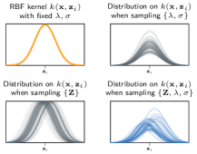
Figure 1: Representation of the induced posterior distribution on the covariance function at location ${\boldsymbol{\mathbf{x}}}$.

Thus, we revisit the role of the inducing inputs in gp models and their treatment as variational parameters or even hyper-parameters. Given their potential high dimensionality and that the typical number of inducing variables goes beyond hundreds/thousands (Shi et al.,, 2019), we argue that they should be treated simply as model variables and, therefore, having priors and carrying out efficient posterior inference over them is an important—although challenging—problem. An illustration of the richer modeling capabilities offered by treating inducing inputs in a Bayesian fashion is given in Fig. 1.

Contributions.  Firstly, we challenge the common wisdom that optimizing the inducing inputs in the variational framework yields optimal performance. We show that, by revisiting old model approximations such as the fully independent training conditionals (fitc; see Quiñonero-Candela and Rasmussen,, 2005) endowed with powerful sampling-based inference methods, treating both inducing locations and gp hyper-parameters in a Bayesian way can improve performance significantly. We describe the conceptual justification and the mathematical details of our general formulation in § 2 and § 3. We then demonstrate that our approach yields state-of-the-art performance across a wide range of competitive benchmark methods, large-scale datasets and a variety of gp and deep gp models (§ 4).

2 BAYESIAN SPARSE GAUSSIAN PROCESSES

We are interested in supervised learning problems with $N$ input-label training pairs $\{{\boldsymbol{\mathbf{X}}},{\boldsymbol{\mathbf{y}}}\}\stackrel{{\scriptstyle\text{def}}}{{=}}\{({\boldsymbol{\mathbf{x}}}_{i},y_{i})\}_{i=1}^{N}$ , where we consider a conditional likelihood $p({\boldsymbol{\mathbf{y}}}\,|\,{\boldsymbol{\mathbf{f}}})$ and ${\boldsymbol{\mathbf{f}}}$ is drawn from a zero-mean gp prior with covariance function $k({\boldsymbol{\mathbf{x}}},{\boldsymbol{\mathbf{x}}}^{\prime};{\boldsymbol{\mathbf{\theta}}})$ with hyper-parameters ${\boldsymbol{\mathbf{\theta}}}$. Thus, we have that $p({\boldsymbol{\mathbf{f}}})=\mathcal{N}(\boldsymbol{\mathbf{0}},{\boldsymbol{\mathbf{K}}}_{\mathrm{xx}|{\boldsymbol{\mathbf{\theta}}}})$, where ${\boldsymbol{\mathbf{K}}}_{\mathrm{xx}|{\boldsymbol{\mathbf{\theta}}}}$ is the $N\times N$ covariance matrix obtained by evaluating $k({\boldsymbol{\mathbf{x}}}_{i},{\boldsymbol{\mathbf{x}}}_{j};{\boldsymbol{\mathbf{\theta}}})$ over all input pairs $\{{\boldsymbol{\mathbf{x}}}_{i},{\boldsymbol{\mathbf{x}}}_{j}\}$. Inference in these types of models generally involves the costly $\mathcal{O}(N^{3})$ operations to compute the inverse and log-determinant of the covariance matrix ${\boldsymbol{\mathbf{K}}}_{\mathrm{xx}|{\boldsymbol{\mathbf{\theta}}}}$.

Full joint distribution of sparse approximations.  Sparse gps are a family of approximate models that address the scalability issue by introducing a set of $M$ inducing variables ${\boldsymbol{\mathbf{u}}}=(u_{1},\ldots,u_{M})$ at corresponding inducing inputs ${\boldsymbol{\mathbf{Z}}}=\{{\boldsymbol{\mathbf{z}}}_{1},\ldots,{\boldsymbol{\mathbf{z}}}_{M}\}$ such that $u_{i}=f({\boldsymbol{\mathbf{z}}}_{i})$ (see, e.g., Quiñonero-Candela and Rasmussen,, 2005). These inducing variables are assumed to be drawn from the same gp as the original process, yielding the joint prior $p({\boldsymbol{\mathbf{f}}},{\boldsymbol{\mathbf{u}}})=p({\boldsymbol{\mathbf{u}}})p({\boldsymbol{\mathbf{f}}}\,|\,{\boldsymbol{\mathbf{u}}})$. In the spirit of Bayesian modeling, any uncertainty in the covariance should be accounted for. Thinking of gp hyper-parameters and inducing inputs as parameters of the covariance function, a distribution over these induces a distribution over the covariance function, which enriches the modeling capabilities of these models (see, e.g., Jang et al., (2017)). We consider a general formulation where we place priors $p_{{\boldsymbol{\mathbf{\psi}}}}({\boldsymbol{\mathbf{\theta}}})$ over covariance hyper-parameters and $p_{{\boldsymbol{\mathbf{\xi}}}}({\boldsymbol{\mathbf{Z}}})$ over inducing inputs with hyper-parameters ${\boldsymbol{\mathbf{\psi}}},{\boldsymbol{\mathbf{\xi}}}$,

$$p({\boldsymbol{\mathbf{\theta}}}, {\boldsymbol{\mathbf{Z}}},{\boldsymbol{\mathbf{u}}},{\boldsymbol{\mathbf{f}}},{\boldsymbol{\mathbf{y}}}\,|\,{\boldsymbol{\mathbf{X}}})=$$ (1)

$$=p_{{\boldsymbol{\mathbf{\psi}}}}({\boldsymbol{\mathbf{\theta}}})p_{\boldsymbol{\mathbf{\xi}}}({\boldsymbol{\mathbf{Z}}})p({\boldsymbol{\mathbf{u}}}\,|\,{\boldsymbol{\mathbf{Z}}},{\boldsymbol{\mathbf{\theta}}})p({\boldsymbol{\mathbf{f}}}\,|\,{\boldsymbol{\mathbf{u}}},{\boldsymbol{\mathbf{X}}},{\boldsymbol{\mathbf{Z}}},{\boldsymbol{\mathbf{\theta}}})p({\boldsymbol{\mathbf{y}}}\,|\,{\boldsymbol{\mathbf{f}}}),$$

where $p({\boldsymbol{\mathbf{u}}}\,|\,{\boldsymbol{\mathbf{Z}}},{\boldsymbol{\mathbf{\theta}}})=\mathcal{N}(\mathbf{0},{\boldsymbol{\mathbf{K}}}_{\mathrm{zz}|{\boldsymbol{\mathbf{\theta}}}})$, $p({\boldsymbol{\mathbf{f}}}\,|\,{\boldsymbol{\mathbf{u}}},{\boldsymbol{\mathbf{X}}},{\boldsymbol{\mathbf{Z}}},{\boldsymbol{\mathbf{\theta}}})=\mathcal{N}({\boldsymbol{\mathbf{K}}}_{\mathrm{xz}|{\boldsymbol{\mathbf{\theta}}}}{\boldsymbol{\mathbf{K}}}_{\mathrm{zz}|{\boldsymbol{\mathbf{\theta}}}}^{-1}{\boldsymbol{\mathbf{u}}},{\boldsymbol{\mathbf{K}}}_{\mathrm{xx}|{\boldsymbol{\mathbf{\theta}}}}-{\boldsymbol{\mathbf{K}}}_{\mathrm{xz}|{\boldsymbol{\mathbf{\theta}}}}{\boldsymbol{\mathbf{K}}}_{\mathrm{zz}|{\boldsymbol{\mathbf{\theta}}}}^{-1}{\boldsymbol{\mathbf{K}}}_{\mathrm{xz}|{\boldsymbol{\mathbf{\theta}}}}^{\top})$. The matrices ${\boldsymbol{\mathbf{K}}}_{\mathrm{zz}|{\boldsymbol{\mathbf{\theta}}}},{\boldsymbol{\mathbf{K}}}_{\mathrm{xz|{\boldsymbol{\mathbf{\theta}}}}}$ denote the covariance matrices computed between points in ${\boldsymbol{\mathbf{Z}}}$ and $\{{\boldsymbol{\mathbf{X}}},{\boldsymbol{\mathbf{Z}}}\}$, respectively. We assume a factorized likelihood $p({\boldsymbol{\mathbf{y}}}\,|\,{\boldsymbol{\mathbf{f}}})=\prod_{n=1}^{N}p(y_{n}\,|\,f_{n})$ and make no assumptions about the other distributions. In this general formulation, approaches that do not consider priors over covariance hyper-parameters or inducing inputs correspond to improper uniform priors in Eq. 1.

2.1 Scalable inference frameworks for GPs

Let ${\boldsymbol{\mathbf{\Psi}}}\stackrel{{\scriptstyle\text{def}}}{{=}}\{{\boldsymbol{\mathbf{u}}},{\boldsymbol{\mathbf{Z}}},{\boldsymbol{\mathbf{\theta}}}\}$ be the variables whose posterior we wish to infer. Our main object of interest is the log joint marginal obtained by integrating out the latent variables ${\boldsymbol{\mathbf{f}}}$ in Eq. 1, i.e., $\log p({\boldsymbol{\mathbf{y}}},{\boldsymbol{\mathbf{\Psi}}}\,|\,{\boldsymbol{\mathbf{X}}})=\log\int_{{\boldsymbol{\mathbf{f}}}}p({\boldsymbol{\mathbf{y}}}\,|\,{\boldsymbol{\mathbf{f}}})p({\boldsymbol{\mathbf{f}}}\,|\,{\boldsymbol{\mathbf{\Psi}}},{\boldsymbol{\mathbf{X}}})\text{d}{\boldsymbol{\mathbf{f}}}+\log p({\boldsymbol{\mathbf{\Psi}}})$. In particular, we are interested in discussing approximations to this that decompose over observations, allowing the use of stochastic optimization techniques to scale up to large datasets. In the literature of sparse gps (see, e.g., Bauer et al.,, 2016; Bui et al.,, 2017), two of the most influential methods for carrying out inference on such models are based on the variational free energy (vfe) framework (Titsias, 2009a, ) and the fully independent training conditional (fitc) framework (Snelson and Ghahramani,, 2006).

VFE approximations.  The key innovation in Titsias, 2009a is the definition of the approximate posterior $q({\boldsymbol{\mathbf{f}}},{\boldsymbol{\mathbf{u}}})\stackrel{{\scriptstyle\text{def}}}{{=}}q({\boldsymbol{\mathbf{u}}})p({\boldsymbol{\mathbf{f}}}\,|\,{\boldsymbol{\mathbf{\Psi}}},{\boldsymbol{\mathbf{X}}})$, where $q({\boldsymbol{\mathbf{u}}})$ is the variational posterior, which yields the evidence lower bound (elbo)

$$p(\mathbf{y}\,|\,{\boldsymbol{\mathbf{X}}},{\boldsymbol{\mathbf{Z}}},{\boldsymbol{\mathbf{\theta}}})\geq$$ (2)

$$-\textsc{kl}\left[q({\boldsymbol{\mathbf{u}}})\;\|\;p({\boldsymbol{\mathbf{u}}}\,|\,{\boldsymbol{\mathbf{Z}}},{\boldsymbol{\mathbf{\theta}}})\right]+\mathbb{E}_{q({\boldsymbol{\mathbf{f}}},{\boldsymbol{\mathbf{u}}})}\log p({\boldsymbol{\mathbf{y}}}\,|\,{\boldsymbol{\mathbf{f}}})\stackrel{{\scriptstyle\text{def}}}{{=}}\mathcal{L}_{\textsc{elbo}}\,.$$

We note that this approach does not incorporate priors over inducing inputs or hyper-parameters. Inference involves constraining $q({\boldsymbol{\mathbf{u}}})$ to a parametric form and finding its parameters to optimize the elbo. Titsias, 2009a correctly argues that in the regression setting the variational approach to inducing variable approximations should be more robust to overfitting than a direct marginal likelihood maximization approach of traditional approximate models such as those described in Quiñonero-Candela and Rasmussen, (2005). Indeed, if inducing inputs ${\boldsymbol{\mathbf{Z}}}$ are optimized then the resulting elbo provides an additional regularization term (see Titsias, 2009a, , §3 for details). However, as we shall see later, the benefits of being Bayesian about the inducing inputs and estimating their posterior distribution can be superior to those obtained by this regularization.

Restricting the form of $q({\boldsymbol{\mathbf{u}}})$ is suboptimal, and Hensman et al., 2015b proposes to sample from the optimal posterior approximation instead. By applying Jensen’s inequality to bound the log joint marginal we obtain the following formulation,

$$\log p({\boldsymbol{\mathbf{y}}},{\boldsymbol{\mathbf{\Psi}}}\,|\,{\boldsymbol{\mathbf{X}}})\geq$$ (3)

$$\mathbb{E}_{p({\boldsymbol{\mathbf{f}}}\,|\,{\boldsymbol{\mathbf{\Psi}}},{\boldsymbol{\mathbf{X}}})}\log p({\boldsymbol{\mathbf{y}}}\,|\,{\boldsymbol{\mathbf{f}}})+\log p({\boldsymbol{\mathbf{\Psi}}})\stackrel{{\scriptstyle\text{def}}}{{=}}\log\widetilde{p}_{\textsc{vfe}}({\boldsymbol{\mathbf{y}}},{\boldsymbol{\mathbf{\Psi}}}\,|\,{\boldsymbol{\mathbf{X}}}).$$

This is the same expression derived in Hensman et al., 2015b , although following a different derivation showing that $\widetilde{p}_{\textsc{vfe}}$ indeed yields the optimal distribution under the vfe framework of Eq. 9. However, Hensman et al., 2015b argues that a Bayesian treatment of inducing inputs is unnecessary and concludes that the optimal prior is $p({\boldsymbol{\mathbf{Z}}})=q({\boldsymbol{\mathbf{Z}}})=\delta({\boldsymbol{\mathbf{Z}}}-\hat{{\boldsymbol{\mathbf{Z}}}})$, where $\delta(\cdot)$ is Dirac’s delta function and $\hat{{\boldsymbol{\mathbf{Z}}}}$ is the set of inducing inputs that maximizes the elbo (Hensman et al., 2015b, , §3). We find such a justification flawed as it contradicts the fundamental principles of Bayesian inference. Indeed, the derivation by Hensman et al., 2015b relies on minimizing both sides of the KL term in Eq. 9, allowing for a ‘free-form’ optimization of the prior, which ultimately negates the necessity of all prior choices and defeats the purpose of a Bayesian treatment.

FITC approximations.  As an alternative, we can approximate the log joint of Eq. 1 by imposing independence in the conditional distribution (see Quiñonero-Candela and Rasmussen,, 2005, for details), i.e.,  parameterizing $p({\boldsymbol{\mathbf{f}}}\,|\,{\boldsymbol{\mathbf{\Psi}}},{\boldsymbol{\mathbf{X}}})=\mathcal{N}\left({\boldsymbol{\mathbf{K}}}_{\mathrm{xz}|{\boldsymbol{\mathbf{\theta}}}}{\boldsymbol{\mathbf{K}}}_{\mathrm{zz}|{\boldsymbol{\mathbf{\theta}}}}^{-1}{\boldsymbol{\mathbf{u}}},\textrm{diag}\left[{\boldsymbol{\mathbf{K}}}_{\mathrm{xx}|{\boldsymbol{\mathbf{\theta}}}}-{\boldsymbol{\mathbf{K}}}_{\mathrm{xz}|{\boldsymbol{\mathbf{\theta}}}}{\boldsymbol{\mathbf{K}}}_{\mathrm{zz}|{\boldsymbol{\mathbf{\theta}}}}^{-1}{\boldsymbol{\mathbf{K}}}_{\mathrm{xz}|{\boldsymbol{\mathbf{\theta}}}}^{\top}\right]\right)$,

$$\log p({\boldsymbol{\mathbf{y}}},{\boldsymbol{\mathbf{\Psi}}}\,|\,{\boldsymbol{\mathbf{X}}})\approx$$

$$\underbrace{\sum\nolimits_{n=1}^{N}\log\mathbb{E}_{p(f_{n}\,|\,{\boldsymbol{\mathbf{\Psi}}},{\boldsymbol{\mathbf{X}}})}\left[p(y_{n}\,|\,f_{n})\right]+\log p({\boldsymbol{\mathbf{\Psi}}})}_{\stackrel{{\scriptstyle\text{def}}}{{=}}\log\tilde{p}_{\textsc{fitc}}({\boldsymbol{\mathbf{y}}},{\boldsymbol{\mathbf{\Psi}}}\,|\,{\boldsymbol{\mathbf{X}}})}.$$ (4)

This same formulation of the fitc objective can be also been obtain by modifying the likelihood or the prior rather then the conditional distribution (Snelson and Ghahramani,, 2006; Titsias, 2009a, ; Bauer et al.,, 2016).

We now see that, when considering i.i.d. conditional likelihoods, both approximations, $\log\tilde{p}_{\textsc{VFE}}$ and $\log\tilde{p}_{\textsc{FITC}}$, yield objectives that decompose on the observations, enabling scalable inference methods. In particular, we aim to sample from the posterior over all the latent variables using scalable approaches such as stochastic gradient Hamiltonian Monte Carlo (sghmc; Chen et al.,, 2014). The main question is what approach should be preferred and how they relate to their optimization counterparts.

2.2 Sampling with VFE or FITC?

We will show in § 4 that our proposal that samples from the posterior according to Eq. 4 consistently outperforms that in Eq. 3. To understand why the fitc objective makes sense we need to go back to the original work of Titsias, 2009a ; Titsias, 2009b and the seminal work of Quiñonero-Candela and Rasmussen, (2005). Indeed, Titsias, 2009b shows that, in the standard regression case with homoskedastic observation noise, vfe yields exactly the same predictive posterior as the projected process (pp) approximation (Seeger et al.,, 2003), which is referred to as the deterministic training conditional (dtc) approximation. Despite this equivalence, as highlighted in Titsias, 2009a , the main difference is that the vfe framework provides a more robust approach to hyper-parameter estimation as the resulting elbo corresponds to a regularized marginal likelihood of the dtc approach. Nevertheless, the dtc/pp, and consequently the vfe, predictive distribution has been shown to be less accurate than the fitc approximation (Titsias, 2009a, ; Quiñonero-Candela and Rasmussen,, 2005; Snelson,, 2007). Effectively, as described by Quiñonero-Candela and Rasmussen, (2005), the vfe’s solution (which is the same as dtc’s) can be understood as considering a deterministic conditional prior $p({\boldsymbol{\mathbf{f}}}\,|\,{\boldsymbol{\mathbf{u}}})$, i.e. a conditional prior with zero variance.

Consequently, the main reason for the superior performance of vfe in earlier approaches, despite providing a less accurate predictive posterior than fitc’s, was that inducing input estimation was less prone to overfitting due to the use of the variational objective, which provided an extra regularization term. However, by placing priors over the inducing inputs ${\boldsymbol{\mathbf{Z}}}$ as well as over covariance hyper-parameters (as we propose in this work), regularization over these parameters becomes unnecessary. For this reason, we expect the log of the expectation in Eq. 4 to provide more accurate results than the expectation of the log in Eq. 3. Finally, it is important to point out that a variational formulation equivalent to fitc has also been proposed (see Titsias, 2009b, , App. C). Our experimental evaluation, also assesses the benefits of our method with respect to that approach. Full details of this analysis can be found in the supplement.

Figure 2: Illustration of a binary classification task on the banana dataset. Left: the decision bounds of the average classifier. Right: the posterior marginals of the inducing inputs.

3 PRACTICAL CONSIDERATIONS AND EXTENSION TO DEEP GPs

In this section we describe practical considerations in our Bayesian sparse Gaussian process (bsgp) framework, including inference techniques, prior choices and extensions to deep Gaussian processes. Recalling that ${\boldsymbol{\mathbf{\Psi}}}=\{{\boldsymbol{\mathbf{\theta}}},{\boldsymbol{\mathbf{u}}},{\boldsymbol{\mathbf{Z}}}\}$ represents the set of variables to infer and, using Eq. 4, their posterior can be obtained as

$$\log p({\boldsymbol{\mathbf{\Psi}}}\,|\,{\boldsymbol{\mathbf{y}}},{\boldsymbol{\mathbf{X}}})= \log\mathbb{E}_{p({\boldsymbol{\mathbf{f}}}\,|\,{\boldsymbol{\mathbf{\Psi}}},{\boldsymbol{\mathbf{X}}})}p({\boldsymbol{\mathbf{y}}}\,|\,{\boldsymbol{\mathbf{f}}})+\log p({\boldsymbol{\mathbf{u}}}\,|\,{\boldsymbol{\mathbf{\theta}}},{\boldsymbol{\mathbf{Z}}})+$$

$$\log p_{\boldsymbol{\mathbf{\xi}}}({\boldsymbol{\mathbf{Z}}})+\log p_{\boldsymbol{\mathbf{\psi}}}({\boldsymbol{\mathbf{\theta}}})-\log C.$$ (5)

We use Markov chain Monte Carlo (mcmc) techniques, in particular stochastic gradient Hamiltonian Monte Carlo (sghmc) (Chen et al.,, 2014; Havasi et al.,, 2018), to obtain samples from the intractable $p({\boldsymbol{\mathbf{\Psi}}}\,|\,{\boldsymbol{\mathbf{y}}},{\boldsymbol{\mathbf{X}}})$. Unlike Hamiltonian Monte Carlo (hmc), which requires computing the exact gradient $\nabla\log p({\boldsymbol{\mathbf{\Psi}}}\,|\,{\boldsymbol{\mathbf{y}}},{\boldsymbol{\mathbf{X}}})$ and the exact unnormalized posterior to evaluate the acceptance (Neal, 2010a, ), sghmc obtains samples from the posterior with stochastic gradients and without evaluating the Metropolis ratio (see supplement for details). With a factorized likelihood $p({\boldsymbol{\mathbf{y}}}|{\boldsymbol{\mathbf{f}}})$ and an energy function $U({\boldsymbol{\mathbf{\Psi}}})=-\log p({\boldsymbol{\mathbf{\Psi}}}\,|\,{\boldsymbol{\mathbf{y}}},{\boldsymbol{\mathbf{X}}})+\log C$, we sample § 3 over minibatches of data.

3.1 Choosing priors

Next, we discuss prior choices for the inducing inputs and covariance hyper-parameters. The inducing inputs ${\boldsymbol{\mathbf{Z}}}$ support the sparse Gaussian process interpolation, which motivates matching the inducing prior to the data distribution $p({\boldsymbol{\mathbf{X}}})$. We begin by proposing a simple Normal (N) prior $p_{N}({\boldsymbol{\mathbf{Z}}})=\prod_{j=1}^{M}\mathcal{N}({\boldsymbol{\mathbf{z}}}_{j}|\mathbf{0},{\boldsymbol{\mathbf{I}}}),$ which matches the mean and variance of the normalized data distribution, and favors inducing inputs toward the baricenter of the data inputs.

We also explore two priors based on point processes, which consider distributions over point sets (González et al.,, 2016). Point processes can induce repulsive effects penalizing configurations where inducing points are clumped together. The determinantal point process (dpp), defined through $p_{D}({\boldsymbol{\mathbf{Z}}})\propto\det{\boldsymbol{\mathbf{K}}}_{\mathrm{zz}|{\boldsymbol{\mathbf{\theta}}}}\,,$ relates the probability of inducing inputs to the volume of space spanned by the covariance (Lavancier et al.,, 2015). dpp is a repulsive point process, which gives higher probabilities to input diversity, controlled by the hyper-parameters ${\boldsymbol{\mathbf{\xi}}}\equiv{\boldsymbol{\mathbf{\theta}}}$. We then consider the Strauss process (see e.g. Daley and Vere-Jones,, 2003; Strauss,, 1975), $p_{S}({\boldsymbol{\mathbf{Z}}})\propto\lambda^{M}\gamma^{\sum_{{\boldsymbol{\mathbf{z}}},{\boldsymbol{\mathbf{z}}}^{\prime}\in{\boldsymbol{\mathbf{Z}}}}\delta(|{\boldsymbol{\mathbf{z}}}-{\boldsymbol{\mathbf{z}}}^{\prime}|<r)},$ where $\lambda>0$ is the intensity, and $0<\gamma\leq 1$ is the repulsion coefficient which decays the prior as a function of the number of input pairs that are within distance $r$. The Strauss prior (S) tends to maintain the minimum distance between inducing inputs, parameterized by ${\boldsymbol{\mathbf{\xi}}}=(\lambda,\gamma,r)$. We finally consider an uninformative uniform prior (U), $\log p_{U}({\boldsymbol{\mathbf{Z}}})=0$, which effectively provides no contribution to the evaluation of the posterior. To gain insights on the choice of these priors, we set up a comparative analysis on the banana dataset (Fig. 2). We observe that the posterior densities on the inducing inputs are multimodal and highly non-Gaussian, further confirming the necessity of free-form inference. Both Strauss and dpp-based priors encourage configurations where the inducing inputs are evenly spread. The Normal and Uniform priors, instead, focus exclusively on aligning the inducing inputs in a way that is sensible to accurately model the intricate classification boundary between the classes. This insight is confirmed by our the extensive experimental validation in § 4.

Prior on covariance hyper-parameters.

Choosing priors on the hyper-parameters has been discussed in previous works on Bayesian inference for gps (see e.g. Filippone and Girolami,, 2014). Throughout this paper, we use the RBF covariance with automatic relevance determination (ard), marginal variance $\sigma$ and independent lengthscales $\lambda_{i}$ per feature (Mackay,, 1994). On these two hyper-parameters we place a lognormal prior with unit variance and means equal to 1 and 0.05 for ${\boldsymbol{\mathbf{\lambda}}}$ and $\sigma$, respectively.

3.2 Extension to deep Gaussian processes

bsgp can be easily extended to deep Gaussian process (dgp) models (Damianou and Lawrence,, 2013), where we compose $L$ sparse gp layers. Each layer is associated with a set of inducing inputs ${\boldsymbol{\mathbf{Z}}}_{\ell}$, inducing variables ${\boldsymbol{\mathbf{u}}}_{\ell}$ and hyper-parameters ${\boldsymbol{\mathbf{\theta}}}_{\ell}$ (Salimbeni and Deisenroth,, 2017). In our notation ${\boldsymbol{\mathbf{\Psi}}}=\{{\boldsymbol{\mathbf{\Psi}}}_{\ell}\}_{\ell=1}^{L}=\{{\boldsymbol{\mathbf{Z}}}_{\ell},{\boldsymbol{\mathbf{u}}}_{\ell},{\boldsymbol{\mathbf{\theta}}}_{\ell}\}_{\ell=\ell}^{L}$. The joint distribution is

$$p\left({\boldsymbol{\mathbf{y}}},{\boldsymbol{\mathbf{\Psi}}}\right)=p\left({\boldsymbol{\mathbf{y}}}\,|\,{\boldsymbol{\mathbf{f}}}_{L}\right)\prod\nolimits_{\ell=1}^{L}p\left({\boldsymbol{\mathbf{f}}}_{\ell}\,|\,{\boldsymbol{\mathbf{f}}}_{\ell-1},{\boldsymbol{\mathbf{\Psi}}}_{\ell}\right)p({\boldsymbol{\mathbf{\Psi}}}_{\ell}),$$ (6)

where we omit dependency on ${\boldsymbol{\mathbf{X}}}$. In contrast to the ‘shallow’ joint distribution in Eq. 1 and posterior in § 3, the ‘hidden’ layers ${\boldsymbol{\mathbf{f}}}_{\ell}$ are marginalized with sampling and propagated up to the final layer $L$ (Salimbeni and Deisenroth,, 2017), which can be marginalized exactly if the likelihood is Gaussian or by quadrature (Hensman et al., 2015a, ). Full details and derivations for this more general case can be found in the supplement.

4 EXPERIMENTS

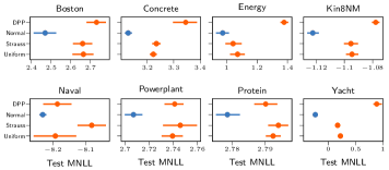
	BSGP with Determinantal Point Process prior (DPP), Strauss process prior, Uniform prior
	BSGP with Normal prior

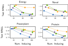
	Gaussian $q({\boldsymbol{\mathbf{u}}})$ [SVGP]
	Free form $p({\boldsymbol{\mathbf{u}}}\,|\,{\boldsymbol{\mathbf{y}}})$ [SGHMC-DGP]
	Free form $p({\boldsymbol{\mathbf{u}}},{\boldsymbol{\mathbf{\theta}}}\,|\,{\boldsymbol{\mathbf{y}}})$
	Free form $p({\boldsymbol{\mathbf{u}}},{\boldsymbol{\mathbf{\theta}}},{\boldsymbol{\mathbf{Z}}}\,|\,{\boldsymbol{\mathbf{y}}})$ [BSGP - THIS WORK]

Figure 3: Left: analysis of different priors on inducing locations for bsgp on the UCI benchmarks: determinantal point process (dpp), Strauss process, uniform. Right: ablation study on the effect of performing posterior inference on different sets of variables. From svgp, where the posterior is constrained to be Gaussian and the remaining parameters are point-estimated, to our proposal bsgp, where we infer a free-form posterior for all ${\boldsymbol{\mathbf{\Psi}}}=\{{\boldsymbol{\mathbf{u}}},{\boldsymbol{\mathbf{\theta}}},{\boldsymbol{\mathbf{Z}}}\}$. We refer the reader to Table 1 for details on the methods (colors are matched).

 

In this section, we provide empirical evidence that our bsgp outperforms previous inference/optimization approaches on shallow and deep gp s. We use eight of the classic UCI benchmark datasets with standardized features and split into eight folds with 0.8/0.2 train/test ratio. We train the competing models for 10,000 iterations with adam (Kingma and Ba,, 2015), step size of 0.01 and a minibatch of 1,000 samples. The sampling methods are evaluated based on 256 samples collected after optimization. Following previous works (e.g. Rasmussen and Williams,, 2006; Havasi et al.,, 2018; Yu et al.,, 2019), in order to evaluate and compare the full predictive posteriors we compute the mean negative loglikelihood (mnll) on the test set (rmses are reported in the supplement for reference).

4.1 Prior analysis and ablation study

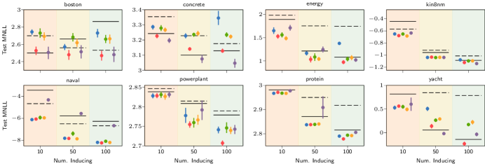
Figure 13: Ablation study on the Test mnll based on the UCI benchmark for different number of inducing variables and for determinantal point process prior ( ), normal prior ( ), Strauss process prior ( ) and uniform prior ( ). These are compared with ( ), corresponding to the case of inducing positions optimized and inducing variables and covariance hyper-parameters sampled, with ( ) where only inducing variables are inferred, while the rest is optimized (similarly to sghmc-dgp). Finally ( ) is the classic svgp, where everything is optimized.

We start our empirical analysis with a comparative evaluation of the priors on inducing inputs described in § 3.1: dpp, Normal, Strauss and Uniform. We run our inference procedure on a shallow gp with 100 inducing points and we report the results in Fig. 13 (left). The results show that the Normal prior consistently outperforms the others. The uniform and Strauss priors behave similarly, while the dpp prior is consistently among the worst. We argue that the repulsive nature of the point process priors (dpp, particularly), although grounded on the intuition of covering the input space more evenly, constrains the smoothness of the functions up to the point that they become too simple to accurately model the data. With this, we select the Gaussian prior for the remaining experiments.

We now study the benefits of a Bayesian treatment of the inducing variables, inducing inputs, and hyper-parameters with an ablation study. Using the same setup as before, we start with the baseline of svgp (Hensman et al.,, 2013; Hensman et al., 2015a, ), where the posterior on ${\boldsymbol{\mathbf{u}}}$ is approximated using a Gaussian and ${\boldsymbol{\mathbf{Z}}},{\boldsymbol{\mathbf{\theta}}}$ are optimized. We then incrementally add parameters to the list of variables that are sampled rather than optimized: only ${\boldsymbol{\mathbf{u}}}$ (equivalent to sghmc-dgp, (Havasi et al.,, 2018)), then $\{{\boldsymbol{\mathbf{u}}},{\boldsymbol{\mathbf{\theta}}}\}$ and finally, our proposal, $\{{\boldsymbol{\mathbf{u}}},{\boldsymbol{\mathbf{\theta}}},{\boldsymbol{\mathbf{Z}}}\}$. This experiment is repeated for different number of inducing points (10, 50 and 100). Fig. 13 (right) reports a summary of these results (full comparison in the supplement). This plot shows that each time we carry out free-form posterior inference on a bigger set of parameters rather than optimization, performance is enhanced, and our proposal outperforms previous approaches.

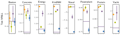
	Inference of ${\boldsymbol{\mathbf{u}}}$ on the variational objective (SVGP – Hensman et al., 2015a, )
	Inference of ${\boldsymbol{\mathbf{u}}}$ with heteroskedastic likelihood (equivalent to FITC) (FITC-SVGP – Titsias, 2009a, )
	MCMC inference of ${\boldsymbol{\mathbf{u}}},{\boldsymbol{\mathbf{\theta}}}$ on the variational objective (MCMC-SVGP – Hensman et al., 2015b, )
	MCMC inference of ${\boldsymbol{\mathbf{u}}},{\boldsymbol{\mathbf{\theta}}}$ on the marginal likelihood (log of expectation)
	MCMC inference of ${\boldsymbol{\mathbf{u}}},{\boldsymbol{\mathbf{\theta}}},{\boldsymbol{\mathbf{Z}}}$ on the marginal likelihood [BSGP - THIS WORK]

Figure 4: Analysis of different choices of objectives when used for optimization and sampling. We refer the reader to Table 1 for a description of the methods.

Figure 5: p-values of the hypothesis test that bsgp with vfe objective is better than bsgp with fitc objective; depth of the dgp from 1 ( ) to 5 ( ). For models with $\text{p-values}<0.05$, we reject the hypothesis.

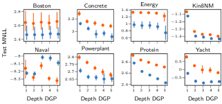
Figure 6: bsgp with the two different objectives for the sampler: fitc ( ) and vfe ( ).

4.2 Choosing the objective: VFE vs FITC

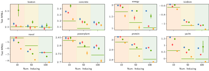
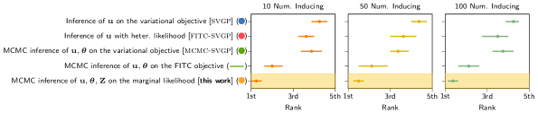
Figure 12: Empirical analysis of different choices of objectives for optimization and sampling.

In § 2 we discussed the role of the marginal and the variational free energy (vfe) objective when used for optimization and for sampling. In Fig. 12 we support the discussion with empirical results. The baseline is svgp, for which the inference is approximate (Gaussian) and performed on the variational objective. Titsias, 2009b (, App. C) also considers a vfe formulation of fitc which corresponds to a gp regression with heteroskedastic noise variance. The likelihood needs to be augmented to handle heteroskedasticity, but inference can be carried out exactly on the variational objective. For these two methods, $\{{\boldsymbol{\mathbf{\theta}}},{\boldsymbol{\mathbf{Z}}}\}$ are optimized. We also test mcmc-svgp, the model proposed by Hensman et al., 2015b , implemented in GPflow (Matthews et al.,, 2017) with the same suggested experimental setup. This experiment indicates that having a free-form posterior on ${\boldsymbol{\mathbf{u}}},{\boldsymbol{\mathbf{\theta}}}$ sampled from the variational objective does not dramatically improve on the exact Gaussian approximation of the fitc model, with both of them delivering superior performance with respect to svgp. In the same setup of Hensman et al., 2015b (${\boldsymbol{\mathbf{u}}},{\boldsymbol{\mathbf{\theta}}}$ sampled and ${\boldsymbol{\mathbf{Z}}}$ optimized), we look at the effect of swapping the expectation of log with the log of expectation (which effectively means moving from the vfe objective to fitc); on the contrary, here we observe a significant increase in performance when using the latter, further confirming the discussion of the objectives in § 2.2. We finally conclude this section with an experiment where we try both objectives on our proposed bsgp and also different depths of the dgp (Fig. 6). Using the Wilcoxon signed-rank test (Wilcoxon,, 1945), we test the null hypothesis of vfe objective being better than the proposed fitc. Fig. 5 shows that, for the majority of the cases, this can be rejected ($p<0.05$).

	BSGP (This work)
	IPVI-DGP
	(Yu et al.,, 2019)
	SGHMC-DGP
	(Havasi et al.,, 2018)
	SVGP
	(Hensman et al., 2015a, )

Figure 7: Test mnll on UCI regression benchmarks (the error bars represent the $95\%$CI). The lower mnll (i.e. to the left), the better. The number on the right of the method’s name refers to the depth of the dgp. Bottom right: Rank summary of all methods.

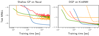
BSGP

IPVI-DGP

SGHMC-DGP

SVGP

Figure 8: Comparison of test mnll as function of training time. The dashed line on the right hand side plot corresponds to svgp with $M=1000$ inducing points.

4.3 Deep Gaussian processes on UCI benchmarks

We now report results on dgps. We compare against two current state-of-the-art deep gp methods, sghmc-dgp (Havasi et al.,, 2018) and ipvi-dgp (Yu et al.,, 2019), and against the shallow svgp baseline (Hensman et al., 2015a, ). For a faithful comparison with ipvi-dgp we follow the recommended parameter configurations. Using a standard setup, all models share $M=100$ inducing points, the same RBF covariance with ard and, for dgp, the same hidden dimensions (equal to the input dimension $D$). Fig. 7 shows the predictive test mnll mean and $95\%$ CI over the different folds over the UCI datasets, and also includes rank summaries. The proposed method clearly outperforms competing deep and shallow gps. The improvements are particularly evident on naval, a dataset known to be challenging to improve upon. Furthermore, the deeper models perform consistently better or on par with the shallow version, without incurring in any measurable overfitting even on small or medium sized datasets (see boston and yacht, for example).

Computational efficiency.  Similarly to the baseline algorithms, each training iteration of bsgp involves the computation of the inverse covariance with complexity $\mathcal{O}(M^{3})$. In Fig. 8 we compare the three main competitors with bsgp trained for a fixed training time budget of one hour for a shallow gp and a 2-layer dgp. The experiment is repeated four times on the same fold and the results are then averaged. Each run is performed on an isolated instance in a cloud computing platform with 8 CPU cores and 8 GB of reserved memory (Pace et al.,, 2017). Inference on the test set is performed every 250 iterations. This shows that bsgp converges considerably faster in wall-clock time, even though a single gradient step requires slightly more time.

Computing the predictive distribution, on the other hand, is more challenging as it requires recomputing the covariance matrices $\mathbf{K}_{\mathrm{xz}},\mathbf{K}_{\mathrm{zz}}$ for each posterior sample $\{{\boldsymbol{\mathbf{Z}}},{\boldsymbol{\mathbf{\theta}}}\}$, for an overall complexity linear in the number of posterior samples. This operation can be easily parallelized and implemented on gpus but it could question the practicality of using a more involved inference method. In particular, it is relevant to study whether svgp could deliver superior performance with a higher number of inducing points for less computational overhead. In Fig. 9 we study this trade-off on the biggest dataset considered (Protein): while it is evident that predictions with bsgp take more time (assuming a serial computation of the covariance matrices), it is also clear that the number of inducing points svgp requires to (even marginally) improve upon bsgp is significantly larger (up to 20 times).

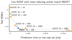
Figure 9: Comparison of test mnll as a function of prediction time on the largest dataset (Protein).

Structured inducing points.  Finally, we run one last comparison with methods which exploit structure in the inputs. These models allow one to scale the number of inducing variables while maintaining computational tractability. Kernel Interpolation for Scalable Structured Gaussian Processes (kiss-gp) (Wilson and Nickisch,, 2015) proposes to place the inducing inputs on a fixed and equally-spaced grid and to exploit Toeplitz/Kronecker structures with an iterative conjugate gradient method to further enhance scalability. Despite these benefits, kiss-gp is known to fall short with high-dimensional data ($D>4$). This shortcoming was later addressed with Deep Kernel Learning (dkl) (Wilson et al., 2016a, ): using a deep neural network dkl projects the data in a lower dimensional manifold by learning an useful feature representation, which is then used as input to a kiss-gp. In Fig. 10 we have the comparison of bsgp with these two methods. kiss-gp could only run on Powerplant, with a 4-dimensional grid of size 10 (for a total of 10,000 inducing points). Here, bsgp delivers better performance despite having less inducing points. For dkl we followed the suggestion of Wilson et al., 2016a to use a fully-connected neural network with a $[d-1000-1000-500-50-2]$ architecture as feature extractor and a grid size of 100 (for again a total of 10,000 inducing points). Training is performed by alternating optimization of the neural network weights and the kiss-gp parameters. Thanks to the flexibility of the feature extractor, this configuration is very competitive with our shallow bsgp, but it yields lower performance compared to a 2-layer dgp.

Figure 10: Comparison with structured inducing variables methods. kiss-gp could only run on the Powerplant dataset (hence the ✗ on Protein and Kin8NM).

4.4 Large scale classification

The airline dataset is a classic benchmark for large scale classification. It collects delay information of all commercial flights in USA during 2008, counting more than 5 millions data points. The goal is to predict if a flight will be delayed based on 8 features, namely month, day of month, day of week, airtime, distance, arrival time, departure time and age of the plane. We pre-process the dataset following the guidelines provided in (Hensman et al., 2015b, ; Wilson et al., 2016a, ).

After a burn-in phase of 10,000 iterations, we draw 200 samples with 1000 simulation steps in between. We test on 100,000 randomly selected held-out points. We fit three models with $M=100$ inducing points. Table 2 shows the predictive performance of three shallow GP models. The bsgp yields the best test error, mnll, and test area under the curve (auc). We assess the convergence of the predictive posterior by evaluating the $\hat{R}$-statistics (Gelman et al.,, 2004) over four independent sghmc chains. This diagnostic yielded a $\hat{R}=1.02\pm 0.045$, which indicates good convergence. We report further convergence analysis in the supplement.

Table 2: airline dataset predictive test performance.

Model	Error ($\downarrow$)	mnll ($\downarrow$)	auc ($\uparrow$)
sghmc-gp	$35.85\%$	$0.646$	$0.671$
svgp	$31.26\%$	$0.595$	$0.730$
bsgp	$\textbf{30.46}\%$	0.580	0.749

As a further large scale example, we use the higgs dataset (Baldi et al.,, 2014), which has 11 millions data points with 28 features. This dataset was created by Monte Carlo simulations of particle dynamics in accelerators to detect the Higgs boson. We select 90% of the these points for training, while the rest is kept for testing. Table 3 reports the final test performance, showing that bsgp outperforms the competing methods. Interestingly, in both these large scale experiments, sghmc-gp always falls back considerably w.r.t. bsgp and even svgp. We argue that, with these large sized datasets, the continuous alternation of optimization of ${\boldsymbol{\mathbf{Z}}}$ and ${\boldsymbol{\mathbf{\theta}}}$ and sampling of ${\boldsymbol{\mathbf{u}}}$ used by the authors (called Moving Window mcem, see Havasi et al., (2018) for details) might have led to suboptimal solutions.

Table 3: higgs dataset predictive test performance.

Model	Error ($\downarrow$)	mnll ($\downarrow$)	auc ($\uparrow$)
sghmc-gp	$35.39\%$	$0.628$	$0.698$
svgp	$27.79\%$	$0.544$	$0.796$
bsgp	$\mathbf{26.97}\%$	$\mathbf{0.530}$	$\mathbf{0.808}$

5 CONCLUSION & DISCUSSION

We have developed a fully Bayesian treatment of sparse Gaussian process models that considers the inducing inputs, along with the inducing variables and covariance hyper-parameters, as random variables, places suitable priors and carries out approximate inference over them. Our approach, based on sghmc, investigated two conventional priors (Gaussian and uniform) for the inducing inputs as well as two point process based priors (the Determinantal and the Strauss processes).

By challenging the standard belief of most previous work on sparse gp inference that assumes the inducing inputs can be estimated point-wisely, we have developed a state-of-the-art inference method and have demonstrated its outstanding performance on both accuracy and running time on regression and classification problems. We hope this work can have an impact similar (or better) to other works in machine learning that have adopted more elaborate Bayesian machinery (e.g. Wallach et al.,, 2009) for long-standing inference problems in commonly used probabilistic models.

Finally, we believe it is worth investigating further more structured priors similar to those presented here (e.g. exploring different hyper-parameter settings), including a full joint treatment of inducing inputs and their number, i.e. $p({\boldsymbol{\mathbf{Z}}},M)$. We leave this for future work. We are currently investigating ways to extend bsgp to convolutional Gaussian process (van der Wilk et al.,, 2017; Dutordoir et al.,, 2019; Blomqvist et al.,, 2020).

Acknowledgements.  MF gratefully acknowledges support from the AXA Research Fund and the Agence Nationale de la Recherche (grant ANR-18-CE46-0002).

Appendix A A Primer on Inference in Sparse GP Models

A gp defines a distribution over functions $f({\boldsymbol{\mathbf{x}}}):\mathbb{R}^{D}\rightarrow\mathbb{R}$ such that for any subset of points $\{{\boldsymbol{\mathbf{x}}}_{1},\ldots,{\boldsymbol{\mathbf{x}}}_{N}\}$ the function values $\{f({\boldsymbol{\mathbf{x}}}_{1}),\ldots,f({\boldsymbol{\mathbf{x}}}_{N})\}$ follow a Gaussian distribution (Rasmussen and Williams,, 2005). A gp is fully described by a mean function $m({\boldsymbol{\mathbf{x}}})$ and a covariance function $\kappa({\boldsymbol{\mathbf{x}}},{\boldsymbol{\mathbf{x}}}^{\prime};{\boldsymbol{\mathbf{\theta}}})$ with hyper-parameters ${\boldsymbol{\mathbf{\theta}}}$. Given a supervised learning problem with $N$ pairs of inputs ${\boldsymbol{\mathbf{x}}}_{i}$ and labels $y_{i}$, $\mathcal{D}=\{({\boldsymbol{\mathbf{x}}}_{i},y_{i})|{\boldsymbol{\mathbf{x}}}_{i}\in\mathbb{R}^{D},y_{i}\in\mathbb{R}\}_{i=1,\dots,N}$, we consider a gp prior over functions which are fed to a suitable likelihood function to model the observed labels.

Denoting by ${\boldsymbol{\mathbf{f}}}\in\mathbb{R}^{N}$ the realizations of the gp random variables at the $N$ inputs ${\boldsymbol{\mathbf{X}}}=\{{\boldsymbol{\mathbf{x}}}_{1},\ldots,{\boldsymbol{\mathbf{x}}}_{N}\}$ and assuming a zero-mean gp prior, we have that $p({\boldsymbol{\mathbf{f}}})=\mathcal{N}(\boldsymbol{\mathbf{0}},{\boldsymbol{\mathbf{K}}}_{\mathrm{xx}|{\boldsymbol{\mathbf{\theta}}}})$, where ${\boldsymbol{\mathbf{K}}}_{\mathrm{xx}|{\boldsymbol{\mathbf{\theta}}}}$ is the covariance matrix obtained by evaluating $\kappa({\boldsymbol{\mathbf{x}}},{\boldsymbol{\mathbf{x}}}^{\prime};{\boldsymbol{\mathbf{\theta}}})$ over all input pairs ${\boldsymbol{\mathbf{x}}}_{i},{\boldsymbol{\mathbf{x}}}_{j}$ (we will drop the explicit parameterization on ${\boldsymbol{\mathbf{\theta}}}$ to keep the notation uncluttered). In the Bayesian setting, given a suitable likelihood function $p({\boldsymbol{\mathbf{y}}}|{\boldsymbol{\mathbf{f}}})$, the objective is to infer the posterior $p({\boldsymbol{\mathbf{f}}}|{\boldsymbol{\mathbf{y}}})$ given $N$ pairs of inputs and labels. This inference problem is analytically tractable for few cases, e.g. using a Gaussian likelihood ${\boldsymbol{\mathbf{y}}}|{\boldsymbol{\mathbf{f}}}\sim\mathcal{N}({\boldsymbol{\mathbf{f}}},\sigma^{2}{\boldsymbol{\mathbf{I}}})$, but it involves the costly $\mathcal{O}(N^{3})$ inversion of the covariance matrix ${\boldsymbol{\mathbf{K}}}_{\mathrm{xx}}$.

Sparse gps are a family of approximate models that address the scalability issue by introducing a set of $M$ inducing variables ${\boldsymbol{\mathbf{u}}}=(u_{1},\ldots,u_{M})$ at corresponding inducing inputs ${\boldsymbol{\mathbf{Z}}}=\{{\boldsymbol{\mathbf{z}}}_{1},\ldots,{\boldsymbol{\mathbf{z}}}_{M}\}$ such that $u=f({\boldsymbol{\mathbf{z}}})$ (Snelson and Ghahramani,, 2005). These inducing variables are assumed to be drawn from the same gp as the original process, yielding the joint prior $p({\boldsymbol{\mathbf{f}}},{\boldsymbol{\mathbf{u}}})=p({\boldsymbol{\mathbf{u}}})p({\boldsymbol{\mathbf{f}}}|{\boldsymbol{\mathbf{u}}})$ with

$$\begin{split}p({\boldsymbol{\mathbf{u}}})&=\mathcal{N}(0,{\boldsymbol{\mathbf{K}}}_{\mathrm{zz}})\\ p({\boldsymbol{\mathbf{f}}}|{\boldsymbol{\mathbf{u}}})&=\mathcal{N}\left({\boldsymbol{\mathbf{K}}}_{\mathrm{xz}}{\boldsymbol{\mathbf{K}}}_{\mathrm{zz}}^{-1}{\boldsymbol{\mathbf{u}}},{\boldsymbol{\mathbf{K}}}_{\mathrm{xx}}-{\boldsymbol{\mathbf{K}}}_{\mathrm{xz}}{\boldsymbol{\mathbf{K}}}_{\mathrm{zz}}^{-1}{\boldsymbol{\mathbf{K}}}_{\mathrm{zx}}\right),\,\end{split}$$ (7)

where ${\boldsymbol{\mathbf{K}}}_{\mathrm{zz}}\equiv k({\boldsymbol{\mathbf{Z}}},{\boldsymbol{\mathbf{Z}}})$, ${\boldsymbol{\mathbf{K}}}_{\mathrm{xz}}\equiv k({\boldsymbol{\mathbf{X}}},{\boldsymbol{\mathbf{Z}}})$ and ${\boldsymbol{\mathbf{K}}}_{\mathrm{xz}}={\boldsymbol{\mathbf{K}}}_{\mathrm{zx}}^{T}$. After introducing the inducing variables, the interest is in obtaining a posterior distribution over ${\boldsymbol{\mathbf{f}}}$ by relying on the set of inducing variables ${\boldsymbol{\mathbf{u}}}$ so as to avoid costly algebraic operations with ${\boldsymbol{\mathbf{K}}}_{\mathrm{xx}}\in\mathbb{R}^{N\times N}$. A general framework to do this for any likelihood and at scale (using mini-batches) can be obtained using variational inference techniques Titsias, 2009a ; Hensman et al., (2013); Bonilla et al., (2019). The main innovation in Titsias, 2009a is the formulation of an approximate posterior $q({\boldsymbol{\mathbf{f}}},{\boldsymbol{\mathbf{u}}})$ within variational inference (Jordan et al.,, 1999) so as to develop such a framework. This variational distribution formulation has come to be known as Titsias’ trick and has the form:

$$q({\boldsymbol{\mathbf{f}}},{\boldsymbol{\mathbf{u}}})=q({\boldsymbol{\mathbf{u}}})p({\boldsymbol{\mathbf{f}}}|{\boldsymbol{\mathbf{u}}}).$$ (8)

Following the variational inference approach, and using the above approximate posterior, we introduce the elbo,

$$\log p(\mathbf{y})\geq-\textsc{kl}\left[q({\boldsymbol{\mathbf{u}}})\;\|\;p({\boldsymbol{\mathbf{u}}})\right]+\mathbb{E}_{q({\boldsymbol{\mathbf{f}}},{\boldsymbol{\mathbf{u}}})}\log p({\boldsymbol{\mathbf{y}}}\,|\,{\boldsymbol{\mathbf{f}}}),$$ (9)

where the Kullback-Leibler divergence (kl) term only involves $M$-dimensional distributions, as the conditional prior (Eq. 7) is also used in the approximate posterior (Eq. 8), which results in the kl involving $N$-dimensional distributions vanish. The second term in the expression above is usually referred to as the expected log likelihood (ell) and, for factorized conditional likelihoods, it can be computed efficiently using quadrature or Monte Carlo (mc) sampling (see, e.g., Hensman et al., 2015a, ). Thus, posterior estimation under this framework involves constraining $q({\boldsymbol{\mathbf{u}}})$ to have a parametric form (usually a Gaussian) and finding its parameters so as to optimize the elbo above. This optimization can be carried out using stochastic-gradient methods operating on mini-batches yielding a time complexity of $O(M^{3})$.

A.1 MCMC for Variationally Sparse GPs

An alternative treatment of the inducing variables under the variational framework described above is to avoid constraining $q({\boldsymbol{\mathbf{u}}})$ to having any parametric form or admitting simplistic factorizing assumptions. As shown by Hensman et al., 2015b , this can be, in fact, achieved by finding the optimal (unconstrained) distribution $q({\boldsymbol{\mathbf{u}}})$ that maximizes the elbo in Eq. 9 and sampling from it using techniques such as mcmc. This optimal distribution can be shown to have the form

$$\log q({\boldsymbol{\mathbf{u}}})=\mathbb{E}_{p({\boldsymbol{\mathbf{f}}}|{\boldsymbol{\mathbf{u}}})}\log p({\boldsymbol{\mathbf{y}}}|{\boldsymbol{\mathbf{f}}})+\log p({\boldsymbol{\mathbf{u}}})+C,$$ (10)

where $C$ is an unknown normalizing constant. This expression makes it apparent that sparse variational gps can be seen as gp models with a Gaussian prior over the inducing variables and a likelihood which has a complicated form due to the expectation under the conditional $p({\boldsymbol{\mathbf{f}}}|{\boldsymbol{\mathbf{u}}})$. This observation makes it possible to derive mcmc samplers for the posterior over ${\boldsymbol{\mathbf{u}}}$, thus relaxing the constraint of having to deal with a fixed form approximation. The only difficulty is that the likelihood requires the computation of an expectation; however, as mentioned above, for most modeling problems where the likelihood factorizes, this expectation can be calculated as a sum of univariate integrals, for which it is easy to employ numerical quadrature. Hensman et al., 2015b also include the sampling of the hyper-parameters ${\boldsymbol{\mathbf{\theta}}}$ jointly with ${\boldsymbol{\mathbf{u}}}$; however, in order to do this efficiently, a whitening representation is employed, whereby the inducing variables are reparameterized as ${\boldsymbol{\mathbf{u}}}={\boldsymbol{\mathbf{L}}}_{\mathrm{zz}}{\boldsymbol{\mathbf{\nu}}}$, with ${\boldsymbol{\mathbf{K}}}_{\mathrm{zz}}={\boldsymbol{\mathbf{L}}}_{\mathrm{zz}}{\boldsymbol{\mathbf{L}}}_{\mathrm{zz}}^{\top}$. The sampling scheme then amounts to sampling from the joint posterior over ${\boldsymbol{\mathbf{\nu}}},{\boldsymbol{\mathbf{\theta}}}$.

The sampling scheme used by Hensman et al., 2015b employs a more efficient method based on Hamiltonian Monte Carlo (hmc, Duane et al.,, 1987; Neal, 2010b, ). Given a potential energy function defined as $U({\boldsymbol{\mathbf{u}}})=-\log p({\boldsymbol{\mathbf{u}}},{\boldsymbol{\mathbf{y}}})=-\log p({\boldsymbol{\mathbf{u}}}|{\boldsymbol{\mathbf{y}}})+C$, hmc introduces auxiliary momentum variables ${\boldsymbol{\mathbf{r}}}$ and it generates samples from the joint distribution $p({\boldsymbol{\mathbf{u}}},{\boldsymbol{\mathbf{r}}})$ by simulation of the Hamiltonian dynamics

$$\mathrm{d}{\boldsymbol{\mathbf{u}}} ={\boldsymbol{\mathbf{M}}}^{-1}{\boldsymbol{\mathbf{r}}}\mathrm{d}t\,,$$

$$\mathrm{d}{\boldsymbol{\mathbf{r}}} =-\nabla U({\boldsymbol{\mathbf{u}}})\mathrm{d}t\,,$$

where ${\boldsymbol{\mathbf{M}}}$ is the so called mass matrix, followed by a Metropolis accept/reject step.

A.2 Stochastic gradient HMC for Deep models

Different from classic hmc where it is required to compute the full gradients $\nabla U({\boldsymbol{\mathbf{u}}})=-\nabla\log p({\boldsymbol{\mathbf{u}}}|{\boldsymbol{\mathbf{y}}})$, sghmc (Chen et al.,, 2014) allows to sample from the true intractable posterior by means of stochastic gradients, and without the need of Metropolis accept/reject steps, which would require access to the whole data set. By modeling the stochastic gradient noise as normally distributed $\mathcal{N}({\boldsymbol{\mathbf{0}}},{\boldsymbol{\mathbf{V}}})$, the (discretized) Hamiltonian dynamics are updated as follows

$${\boldsymbol{\mathbf{u}}}_{t+1} ={\boldsymbol{\mathbf{u}}}_{t+1}+\varepsilon{\boldsymbol{\mathbf{M}}}^{-1}{\boldsymbol{\mathbf{r}}}_{t}\,,$$

$${\boldsymbol{\mathbf{r}}}_{t+1} ={\boldsymbol{\mathbf{r}}}_{t}-\varepsilon\widetilde{\nabla U}({\boldsymbol{\mathbf{u}}})-\varepsilon{\boldsymbol{\mathbf{C}}}{\boldsymbol{\mathbf{M}}}^{-1}{\boldsymbol{\mathbf{r}}}_{t}+\mathcal{N}(0,2\varepsilon({\boldsymbol{\mathbf{C}}}-\tilde{\boldsymbol{\mathbf{B}}}))\,,$$

where $\varepsilon$ is the step size, ${\boldsymbol{\mathbf{C}}}$ is a user defined friction term and $\tilde{\boldsymbol{\mathbf{B}}}$ is the estimated diffusion matrix of the gradient noise; see e.g., Springenberg et al., (2016) for ideas on how to estimate these parameters.

sghmc is the primary inference method used by Havasi et al., (2018) for obtaining samples from the posterior distribution over the latent variables. Recently, this has been approached using adversarial inference methods (Yu et al.,, 2019).

A.3 Other Approaches to Scalable and Bayesian GPs

It is worth mentioning that other approaches to scalable inference in gps have been proposed, which feature the possibility to operate using mini-batches. For example, looking at the feature-space view of kernel machines, Rahimi and Recht, (2008) show how random features can be obtained for shift invariant covariance functions, like the commonly used squared exponential. These approximations are also useful for addressing the scalability of gps and dgps, as showed by Lázaro-Gredilla et al., (2010) and Cutajar et al., (2017). Similarly, the work on structured approximations of gps Saatçi, (2011) has found applications to develop a scalable framework for gps, later developed to include the possibility to learn deep learning-based representations for the input Wilson et al., 2016b .

The Gaussian process latent variable model (gplvm) proposed by Lawrence, (2005) is a popular approach to Bayesian nonlinear dimensionality reduction and its Bayesian extensions such as those develped by Titsias and Lawrence, (2010) consider a prior over the inputs of a gp. Although these methods can be used for training gps with missing or uncertain inputs, we are not aware of previous work adopting such methodologies for inducing inputs within scalable sparse gp models.

Appendix B Discussion on the objectives: VFE vs FITC

To understand why the fitc objective makes sense we need to go back to the original work of Titsias, 2009a ; Titsias, 2009b and the seminal work of Quiñonero-Candela and Rasmussen, (2005). For this, we will consider the regression case and then we can easily generalize our reasoning to the classification case. Titsias, 2009b shows that, in the standard regression case with isotropic observation noise, his vfe optimization framework yields exactly the same predictive posterior as the pp approximation (Seeger et al.,, 2003), which is referred to as the dtc approximation in Quiñonero-Candela and Rasmussen, (2005). The optimal variational posterior distribution is given by:

$$\begin{split}q^{*}({\boldsymbol{\mathbf{u}}}\,|\,{\boldsymbol{\mathbf{\theta}}})&=\mathcal{N}({\boldsymbol{\mathbf{u}}};{\boldsymbol{\mathbf{m}}},{\boldsymbol{\mathbf{S}}}),\\ {\boldsymbol{\mathbf{m}}}&=\sigma^{-2}{\boldsymbol{\mathbf{K}}}_{\mathrm{zz}}{\boldsymbol{\mathbf{\Sigma}}}{\boldsymbol{\mathbf{K}}}_{\mathrm{zx}}{\boldsymbol{\mathbf{y}}}\\ {\boldsymbol{\mathbf{S}}}&={\boldsymbol{\mathbf{K}}}_{\mathrm{zz}}{\boldsymbol{\mathbf{\Sigma}}}{\boldsymbol{\mathbf{K}}}_{\mathrm{zz}},\text{ where }\\ {\boldsymbol{\mathbf{\Sigma}}}&=\left({\boldsymbol{\mathbf{K}}}_{\mathrm{zz}}+\sigma^{-2}{\boldsymbol{\mathbf{K}}}_{\mathrm{zx}}{\boldsymbol{\mathbf{K}}}_{\mathrm{xz}}\right)^{-1},\end{split}$$ (11)

where $\sigma^{2}$ is the observation-noise variance. It is easy to show that, given a Gaussian posterior over the inducing variables with mean and covariance ${\boldsymbol{\mathbf{m}}}$ and ${\boldsymbol{\mathbf{S}}}$, the posterior predictive distribution at test point ${\boldsymbol{\mathbf{x}}}_{\star}$ is a Gaussian with mean and variance

$$\begin{split}\mu_{y}({\boldsymbol{\mathbf{x}}}_{\star})&=\kappa({\boldsymbol{\mathbf{x}}}_{\star},{\boldsymbol{\mathbf{Z}}}){\boldsymbol{\mathbf{K}}}_{\mathrm{zz}}^{-1}{\boldsymbol{\mathbf{m}}}\\ \sigma_{y}^{2}({\boldsymbol{\mathbf{x}}}_{\star})&=\kappa({\boldsymbol{\mathbf{x}}}_{\star},{\boldsymbol{\mathbf{x}}}_{\star})-\kappa({\boldsymbol{\mathbf{x}}}_{\star},{\boldsymbol{\mathbf{Z}}}){\boldsymbol{\mathbf{K}}}_{\mathrm{zz}}^{-1}\kappa({\boldsymbol{\mathbf{Z}}},{\boldsymbol{\mathbf{x}}}_{\star})+\kappa({\boldsymbol{\mathbf{x}}}_{\star},{\boldsymbol{\mathbf{Z}}}){\boldsymbol{\mathbf{K}}}_{\mathrm{zz}}^{-1}{\boldsymbol{\mathbf{S}}}{\boldsymbol{\mathbf{K}}}_{\mathrm{zz}}^{-1}\kappa({\boldsymbol{\mathbf{Z}}},{\boldsymbol{\mathbf{x}}}_{\star}).\end{split}$$ (12)

Thus, replacing Eq. 11 in Eq. 12 we obtain:

$$\begin{split}\mu_{y}({\boldsymbol{\mathbf{x}}}_{\star})&=\sigma^{-2}\kappa({\boldsymbol{\mathbf{x}}}_{\star},{\boldsymbol{\mathbf{Z}}}){\boldsymbol{\mathbf{\Sigma}}}{\boldsymbol{\mathbf{K}}}_{\mathrm{zx}}{\boldsymbol{\mathbf{y}}}\\ \sigma_{y}^{2}({\boldsymbol{\mathbf{x}}}_{\star})&=\kappa({\boldsymbol{\mathbf{x}}}_{\star},{\boldsymbol{\mathbf{x}}}_{\star})-\kappa({\boldsymbol{\mathbf{x}}}_{\star},{\boldsymbol{\mathbf{Z}}}){\boldsymbol{\mathbf{K}}}_{\mathrm{zz}}^{-1}\kappa({\boldsymbol{\mathbf{Z}}},{\boldsymbol{\mathbf{x}}}_{\star})+\kappa({\boldsymbol{\mathbf{x}}}_{\star},{\boldsymbol{\mathbf{Z}}}){\boldsymbol{\mathbf{\Sigma}}}\kappa({\boldsymbol{\mathbf{Z}}},{\boldsymbol{\mathbf{x}}}_{\star}),\end{split}$$ (13)

which indeed corresponds to the predictive distribution of the dtc/pp approximation. Despite this equivalence, as highlighted in Titsias, 2009a , the main difference is that the vfe framework provides a more robust approach to hyper-parameter estimation as the resulting elbo corresponds to a regularized marginal likelihood of the dtc approach and hence should be more robust to overfitting. Nevertheless, the dtc/pp, and consequently the vfe, predictive distribution has been shown to be less accurate than the fitc approximation (Titsias, 2009a, ; Quiñonero-Candela and Rasmussen,, 2005; Snelson,, 2007).

B.1 The FITC Approximation

The fitc approximation considers the following approximate conditional prior:

$$p({\boldsymbol{\mathbf{f}}}\,|\,{\boldsymbol{\mathbf{u}}}) \approx\mathcal{N}\left({\boldsymbol{\mathbf{f}}};{\boldsymbol{\mathbf{K}}}_{\mathrm{xz}}{\boldsymbol{\mathbf{K}}}_{\mathrm{zz}}^{-1}{\boldsymbol{\mathbf{u}}},\textrm{diag}\left({\boldsymbol{\mathbf{K}}}_{\mathrm{xx}}-{\boldsymbol{\mathbf{K}}}_{\mathrm{xz}}{\boldsymbol{\mathbf{K}}}_{\mathrm{zz}}^{-1}{\boldsymbol{\mathbf{K}}}_{\mathrm{zx}}\right)\right)$$

$$=\prod_{n=1}^{N}p(f_{n}\,|\,{\boldsymbol{\mathbf{u}}})=\prod_{n=1}^{N}\mathcal{N}(f_{n};\tilde{\mu}_{n},\tilde{\sigma}_{n}^{2}),\text{ with }$$

$$\tilde{\mu}_{n} =\kappa({\boldsymbol{\mathbf{x}}}_{n},{\boldsymbol{\mathbf{Z}}}){\boldsymbol{\mathbf{K}}}_{\mathrm{zz}}^{-1}{\boldsymbol{\mathbf{u}}}$$ (14)

$$\tilde{\sigma}_{n}^{2} =\kappa({\boldsymbol{\mathbf{x}}}_{n},{\boldsymbol{\mathbf{x}}}_{n})-\kappa({\boldsymbol{\mathbf{x}}}_{n},{\boldsymbol{\mathbf{Z}}}){\boldsymbol{\mathbf{K}}}_{\mathrm{zz}}^{-1}\kappa({\boldsymbol{\mathbf{Z}}},{\boldsymbol{\mathbf{x}}}_{n})\text{.}$$ (15)

As we shall see later, is this factorization assumption in the conditional prior that will yield a decomposable objective amenable to stochastic gradient techniques. For now, consider the posterior predictive distribution under the fitc approximation

$$\begin{split}\mu_{\lx@glossaries@gls@link{acronym}{FITC}{\leavevmode\textsc{fitc}}}({\boldsymbol{\mathbf{x}}}_{\star})&=\kappa({\boldsymbol{\mathbf{x}}}_{\star},{\boldsymbol{\mathbf{Z}}}){\boldsymbol{\mathbf{\Sigma}}}_{\lx@glossaries@gls@link{acronym}{FITC}{\leavevmode\textsc{fitc}}}{\boldsymbol{\mathbf{K}}}_{\mathrm{zx}}{\boldsymbol{\mathbf{\Lambda}}}^{-1}{\boldsymbol{\mathbf{y}}}\\ \sigma^{2}_{\lx@glossaries@gls@link{acronym}{FITC}{\leavevmode\textsc{fitc}}}({\boldsymbol{\mathbf{x}}}_{\star})&=\kappa({\boldsymbol{\mathbf{x}}}_{\star},{\boldsymbol{\mathbf{x}}}_{\star})-\kappa({\boldsymbol{\mathbf{x}}}_{\star},{\boldsymbol{\mathbf{Z}}}){\boldsymbol{\mathbf{K}}}_{\mathrm{zz}}^{-1}\kappa({\boldsymbol{\mathbf{Z}}},{\boldsymbol{\mathbf{x}}}_{\star})+\kappa({\boldsymbol{\mathbf{x}}}_{\star},{\boldsymbol{\mathbf{Z}}}){\boldsymbol{\mathbf{\Sigma}}}_{\lx@glossaries@gls@link{acronym}{FITC}{\leavevmode\textsc{fitc}}}\kappa({\boldsymbol{\mathbf{Z}}},{\boldsymbol{\mathbf{x}}}_{\star}),\text{ where }\\ {\boldsymbol{\mathbf{\Lambda}}}&=\textrm{diag}({\boldsymbol{\mathbf{K}}}_{\mathrm{xx}}-{\boldsymbol{\mathbf{K}}}_{\mathrm{xz}}{\boldsymbol{\mathbf{K}}}_{\mathrm{zz}}^{-1}{\boldsymbol{\mathbf{K}}}_{\mathrm{zx}}+\sigma^{2}{\boldsymbol{\mathbf{I}}})\text{ and }\\ {\boldsymbol{\mathbf{\Sigma}}}_{\lx@glossaries@gls@link{acronym}{FITC}{\leavevmode\textsc{fitc}}}&=({\boldsymbol{\mathbf{K}}}_{\mathrm{zz}}+{\boldsymbol{\mathbf{K}}}_{\mathrm{zx}}{\boldsymbol{\mathbf{\Lambda}}}^{-1}{\boldsymbol{\mathbf{K}}}_{\mathrm{xz}})^{-1}.\end{split}$$ (16)

We now see why fitc’s predictive distribution above is more accurate than vfe’s in Eq. 13, as we can obtain fitc’s by replacing $\sigma^{2}{\boldsymbol{\mathbf{I}}}$ in vfe’s solution with $\textrm{diag}({\boldsymbol{\mathbf{K}}}_{\mathrm{xx}}-{\boldsymbol{\mathbf{K}}}_{\mathrm{xz}}{\boldsymbol{\mathbf{K}}}_{\mathrm{zz}}^{-1}{\boldsymbol{\mathbf{K}}}_{\mathrm{zx}})+\sigma^{2}{\boldsymbol{\mathbf{I}}}$. Effectively, as described in Quiñonero-Candela and Rasmussen, (2005), vfe’s solution (which is the same as dtc’s) can be understood as considering a deterministic conditional prior $p({\boldsymbol{\mathbf{f}}}\,|\,{\boldsymbol{\mathbf{u}}})$, i.e. with zero variance.

B.2 Stochastic Updates Using the FITC Approximation

Now we can understand why the log of the expectation can provide more accurate results than the expectation of the log. Basically in the former we are using the fitc approximation while in the later we are using the vfe/dtc/pp approximation. It is easy to show that when using the fitc approximation, one can obtain a decomposable objective function that can be implemented at large scale using stochastic gradient techniques. Here we focus only on the expectation of the conditional likelihood (which is the crucial term) and in the regression setting for simplicity but the extension to the classification case (e.g. using quadrature) is straightforward.

$$\log p({\boldsymbol{\mathbf{y}}},{\boldsymbol{\mathbf{u}}}\,|\,{\boldsymbol{\mathbf{\theta}}}) =\log\mathbb{E}_{p({\boldsymbol{\mathbf{f}}}\,|\,{\boldsymbol{\mathbf{u}}},{\boldsymbol{\mathbf{\theta}}})}\left[p({\boldsymbol{\mathbf{y}}}\,|\,{\boldsymbol{\mathbf{f}}}\right)]$$

$$=\log\int_{{\boldsymbol{\mathbf{f}}}}p({\boldsymbol{\mathbf{f}}}\,|\,{\boldsymbol{\mathbf{u}}},{\boldsymbol{\mathbf{\theta}}})p({\boldsymbol{\mathbf{y}}}\,|\,{\boldsymbol{\mathbf{f}}})\operatorname{d}\!{{\boldsymbol{\mathbf{f}}}}{\text{\quad will drop ${\boldsymbol{\mathbf{\theta}}}$ for simplicity from now on}}$$

$$=\log\int_{f_{1},\dots,f_{N}}\prod_{n=1}^{N}p(y_{n}\,|\,f_{n})p(f_{n}\,|\,{\boldsymbol{\mathbf{u}}})\operatorname{d}\!{{\boldsymbol{\mathbf{f}}}}$$

$$=\log\prod_{n=1}^{N}\int_{f_{n}}\mathcal{N}(y_{n};f_{n},\sigma^{2})\mathcal{N}(f_{n};\tilde{\mu}_{n},\tilde{\sigma}^{2}_{n})\operatorname{d}\!{f_{n}}$$

$$=\log\prod_{n=1}^{N}p(y_{n}\,|\,{\boldsymbol{\mathbf{u}}})$$

$$=\sum_{n=1}^{N}\log\mathcal{N}(y_{n};\tilde{\mu}_{n},\tilde{\sigma}_{n}^{2}+\sigma^{2}),$$ (17)

where $\tilde{\mu}_{n},\tilde{\sigma}_{n}^{2}$ are given by Eq. 14 and Eq. 15.

Binary classification.

Similar results can be derived for binary classification with Bernoulli likelihood and response function $\lambda(f)$:

$$\log p({\boldsymbol{\mathbf{y}}},{\boldsymbol{\mathbf{u}}}\,|\,{\boldsymbol{\mathbf{\theta}}})=\log\mathbb{E}_{p({\boldsymbol{\mathbf{f}}}\,|\,{\boldsymbol{\mathbf{u}}},{\boldsymbol{\mathbf{\theta}}})}\left[p({\boldsymbol{\mathbf{y}}}\,|\,{\boldsymbol{\mathbf{f}}}\right)]=\log\prod_{n=1}^{N}\int_{f_{n}}\mathcal{N}(f_{n};\tilde{\mu}_{n},\tilde{\sigma}^{2}_{n})\text{Bern}(y_{n};\lambda(f_{n}))\operatorname{d}\!{f_{n}}.$$ (18)

When the response function is the cdf of a standard Normal distribution, i.e., $\lambda(f_{n})=\Phi(f_{n})\stackrel{{\scriptstyle\text{def}}}{{=}}\int_{-\infty}^{f_{n}}\mathcal{N}(f_{n};0,1)df_{n}$, which is also known as the probit regression model, the expectation above can be computed analytically to obtain:

$$\log p({\boldsymbol{\mathbf{y}}},{\boldsymbol{\mathbf{u}}}\,|\,{\boldsymbol{\mathbf{\theta}}})=\sum_{n=1}^{N}\log\text{Bern}(y_{n};\Phi(\tilde{\mu}_{n}/\sqrt{1+\tilde{\sigma}_{n}^{2}})).$$ (19)

For other response functions the expectation in Eq. 18 can be estimated using quadrature.

B.3 An heteroskedastic version of the Gaussian likelihood

As Titsias, 2009b discussed in Appendix C, the fitc approximation corresponds to a gp regression with heteroskedastic noise variance

$$p({\boldsymbol{\mathbf{y}}}|{\boldsymbol{\mathbf{f}}}) =\mathcal{N}({\boldsymbol{\mathbf{y}}}|{\boldsymbol{\mathbf{f}}},\sigma^{2}{\boldsymbol{\mathbf{I}}}+\textrm{diag}[{\boldsymbol{\mathbf{K}}}_{{\boldsymbol{\mathbf{x}}}{\boldsymbol{\mathbf{x}}}}-{\boldsymbol{\mathbf{K}}}_{{\boldsymbol{\mathbf{x}}}{\boldsymbol{\mathbf{z}}}}{\boldsymbol{\mathbf{K}}}_{{\boldsymbol{\mathbf{z}}}{\boldsymbol{\mathbf{z}}}}{\boldsymbol{\mathbf{K}}}_{{\boldsymbol{\mathbf{z}}}{\boldsymbol{\mathbf{x}}}}]).$$ (20)

If we apply this augmented likelihood to the variational expectations term, we get

$$\mathbb{E}_{q({\boldsymbol{\mathbf{f}}})}\log p({\boldsymbol{\mathbf{y}}}|{\boldsymbol{\mathbf{f}}},\sigma^{2},{\boldsymbol{\mathbf{\theta}}}) =-\frac{1}{2}\sum_{j=1}^{n}\left(\log 2\pi(\sigma^{2}+\tilde{\sigma}_{j}^{2})+\frac{(y_{j}-\tilde{\mu}_{j})^{2}+\tilde{\sigma}_{j}^{2}}{\sigma^{2}+\tilde{\sigma}_{j}^{2}}\right).$$ (21)

Since Titsias, 2009b considers this vfe formulation, we also compare with it.

B.4 Concluding remarks

The main reasoning in Titsias, 2009a ’s work behind the better performance of vfe, despite providing a less accurate predictive posterior than fitc’s, was that hyper-parameter estimation was more robust due to the use of the variational objective (which provided an extra regularization term). Now, we have a better way to do inference on hyper-parameters and inducing inputs by placing priors on those and by carrying out free-form inference upon them with sghmc.

Appendix C Extension to Deep Gaussian Processes

In this section, we derive the mathematical basis for of Bayesian treatment of inducing inputs in a dgp setting (Damianou and Lawrence,, 2013). We assume a deep Gaussian process prior $f^{L}\circ f^{L-1}\circ\cdots f^{1}$, where each $f^{l}$ is a gp. For notational brevity, we use ${\boldsymbol{\mathbf{\theta}}}^{l}$ as both kernel hyper-parameters and inducing inputs of the $l$-th layer, and ${\boldsymbol{\mathbf{f}}}^{0}$ as the input vector ${\boldsymbol{\mathbf{X}}}$. Then we can write down the joint distribution over visible and latent variables (omitting the dependency on ${\boldsymbol{\mathbf{X}}}$ for clarity) as

$$p\left({\boldsymbol{\mathbf{y}}},\left\{{\boldsymbol{\mathbf{f}}}^{l},{\boldsymbol{\mathbf{u}}}^{l},{\boldsymbol{\mathbf{\theta}}}^{l}\right\}_{l=1}^{L}\right)=p\left({\boldsymbol{\mathbf{y}}}\,\middle|\,{\boldsymbol{\mathbf{f}}}^{L}\right)\prod_{l=1}^{L}p\left({\boldsymbol{\mathbf{f}}}^{l}\,\middle|\,{\boldsymbol{\mathbf{u}}}^{l},{\boldsymbol{\mathbf{f}}}^{l-1},{\boldsymbol{\mathbf{\theta}}}^{l}\right)p\left({\boldsymbol{\mathbf{u}}}^{l}\,\middle|\,{\boldsymbol{\mathbf{\theta}}}^{l}\right)p\left({\boldsymbol{\mathbf{\theta}}}^{l}\right).$$ (22)

Our goal is to estimate the posterior,

$$\log\widetilde{p}\left(\left\{{\boldsymbol{\mathbf{u}}}^{l},{\boldsymbol{\mathbf{\theta}}}^{l}\right\}_{l=1}^{L}\,\middle|\,{\boldsymbol{\mathbf{y}}}\right)=$$

$$\quad=\log\mathbb{E}_{p\left(\left\{{\boldsymbol{\mathbf{f}}}^{l}\right\}\,\middle|\,\left\{{\boldsymbol{\mathbf{u}}}^{l},{\boldsymbol{\mathbf{\theta}}}^{l}\right\}\right)}p\left({\boldsymbol{\mathbf{y}}}\,\middle|\,{\boldsymbol{\mathbf{f}}}^{L}\right)+\sum_{l=1}^{L}\left(\log p\left({\boldsymbol{\mathbf{u}}}^{l}\,\middle|\,{\boldsymbol{\mathbf{\theta}}}^{l}\right)+\log p\left({\boldsymbol{\mathbf{\theta}}}^{l}\right)\right)-\log C.$$ (23)

Here $C$ is a normalizing constant, after integrating out ${\{{\boldsymbol{\mathbf{f}}}^{l},{\boldsymbol{\mathbf{u}}}^{l},{\boldsymbol{\mathbf{\theta}}}^{l}\}_{l=1}^{L}}$ from the joint. While the distribution $\widetilde{p}$ is intractable, we have obtained the form of its (un-normalized) log joint, from which we can sample using hmc methods. However, Eq. 23 is not immediately computable owing to the intractable expectation term. More calculations reveal that we can, nevertheless, obtain estimates of this expectation term with Monte Carlo sampling

$$\log\mathbb{E}_{p\left(\left\{{\boldsymbol{\mathbf{f}}}^{l}\right\}\,\middle|\,\left\{{\boldsymbol{\mathbf{u}}}^{l},{\boldsymbol{\mathbf{\theta}}}^{l}\right\}\right)}p\left({\boldsymbol{\mathbf{y}}}\,\middle|\,{\boldsymbol{\mathbf{f}}}^{L}\right)\approx$$

$$\qquad\approx\log\mathbb{E}_{p\left(\left\{{\boldsymbol{\mathbf{f}}}^{l}\right\}_{l=2}^{L}\,\middle|\,\widetilde{{\boldsymbol{\mathbf{f}}}}^{1},\left\{{\boldsymbol{\mathbf{u}}}^{l},{\boldsymbol{\mathbf{\theta}}}^{l}\right\}_{l=2}^{L}\right)}p\left({\boldsymbol{\mathbf{y}}}\,\middle|\,{\boldsymbol{\mathbf{f}}}^{L}\right),\quad\widetilde{{\boldsymbol{\mathbf{f}}}}^{1}\sim p\left({\boldsymbol{\mathbf{f}}}^{1}\,\middle|\,{\boldsymbol{\mathbf{u}}}^{1},{\boldsymbol{\mathbf{\theta}}}^{1},{\boldsymbol{\mathbf{f}}}^{0}\right),$$

$$\qquad\approx\log\mathbb{E}_{p\left(\left\{{\boldsymbol{\mathbf{f}}}^{l}\right\}_{l=3}^{L}\,\middle|\,\widetilde{{\boldsymbol{\mathbf{f}}}}^{2},\left\{{\boldsymbol{\mathbf{u}}}^{l},{\boldsymbol{\mathbf{\theta}}}^{l}\right\}_{l=3}^{L}\right)}p\left({\boldsymbol{\mathbf{y}}}\,\middle|\,{\boldsymbol{\mathbf{f}}}^{L}\right),\quad\widetilde{{\boldsymbol{\mathbf{f}}}}^{2}\sim p\left({\boldsymbol{\mathbf{f}}}^{2}\,\middle|\,{\boldsymbol{\mathbf{u}}}^{2},{\boldsymbol{\mathbf{\theta}}}^{2},\widetilde{{\boldsymbol{\mathbf{f}}}}^{1}\right),$$

$$\qquad\approx\ldots$$

$$\qquad\approx\log\mathbb{E}_{p\left({\boldsymbol{\mathbf{f}}}^{L}\,\middle|\,\widetilde{{\boldsymbol{\mathbf{f}}}}^{L-1},{\boldsymbol{\mathbf{u}}}^{L},{\boldsymbol{\mathbf{\theta}}}^{L}\right)}p\left({\boldsymbol{\mathbf{y}}}\,\middle|\,{\boldsymbol{\mathbf{f}}}^{L}\right),\quad\widetilde{{\boldsymbol{\mathbf{f}}}}^{L-1}\sim p\left({\boldsymbol{\mathbf{f}}}^{L-1}\left|{\boldsymbol{\mathbf{u}}}^{L-1},{\boldsymbol{\mathbf{\theta}}}^{L-1},\widetilde{{\boldsymbol{\mathbf{f}}}}^{L-2}\right.\right),$$

$$\qquad=\sum_{n=1}^{N}\log\mathbb{E}_{p\left(f_{n}^{L}\,\middle|\,\widetilde{f}_{n}^{L-1},{\boldsymbol{\mathbf{u}}}^{L},{\boldsymbol{\mathbf{\theta}}}^{L}\right)}p\left(y_{n}\,\middle|\,f_{n}^{L}\right)$$ (24)

Because of the layer-wise factorization of the joint likelihood (Eq. 22), each step of the approximation is unbiased. While it is possible to approximate the last-layer expectation with a Monte Carlo sample $\widetilde{f}_{j}^{L}$, the expectation is tractable when $y_{j}\,|\,f_{j}^{L}$ is a Gaussian or a Bernoulli distribution with a probit regression model, or is computable with one-dimensional quadrature (Hensman et al., 2015b, ).

Appendix D Additional Results

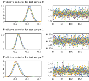
Figure 11: Traces for three test points on the Airline dataset (4 chains/200 samples).

Table 4: Datasets used, including number of datapoints and their dimensionality.

name	n.	d-in	d-out
boston	506	13	1
concrete	1,030	8	1
energy	768	8	2
kin8nm	8,192	8	1
naval	11,934	16	2
powerplant	9,568	4	1
protein	45,730	9	1
yacht	308	6	1
airline	5,934,530	8	2
higgs	11,000,000	28	2

Table 5: Tabular version of Figure 7 in the main paper.

	test mnll
dataset	boston	concrete	energy	kin8nm	naval	powerplant	protein	yacht
name
bsgp 1	$2.47$ ($0.16$)	$3.12$ ($0.04$)	$0.97$ ($0.13$)	$-1.12$ ($0.01$)	$-8.22$ ($0.04$)	$2.71$ ($0.02$)	$2.78$ ($0.01$)	$-0.23$ ($0.13$)
bsgp 2	$2.47$ ($0.15$)	$3.04$ ($0.05$)	$0.95$ ($0.16$)	$-1.40$ ($0.01$)	$-8.23$ ($0.04$)	$2.67$ ($0.02$)	$2.63$ ($0.02$)	$-0.72$ ($0.15$)
bsgp 3	$2.47$ ($0.14$)	$2.96$ ($0.10$)	$0.95$ ($0.15$)	$-1.41$ ($0.01$)	$-8.02$ ($0.04$)	$2.66$ ($0.03$)	$2.57$ ($0.03$)	$-0.83$ ($0.10$)
bsgp 4	$2.48$ ($0.14$)	$2.97$ ($0.06$)	$0.92$ ($0.14$)	$-1.43$ ($0.02$)	$-8.03$ ($0.05$)	$2.65$ ($0.05$)	$2.50$ ($0.03$)	$-0.76$ ($0.13$)
bsgp 5	$2.48$ ($0.12$)	$2.91$ ($0.08$)	$0.75$ ($0.30$)	$-1.43$ ($0.01$)	$-8.09$ ($0.05$)	$2.65$ ($0.03$)	$2.43$ ($0.03$)	$-0.74$ ($0.08$)
ipvi gp 1	$2.84$ ($0.36$)	$3.19$ ($0.11$)	$1.27$ ($0.07$)	$-1.12$ ($0.02$)	$-5.96$ ($0.89$)	$2.79$ ($0.03$)	$2.81$ ($0.02$)	$1.21$ ($1.50$)
ipvi gp 2	$2.73$ ($0.35$)	$3.13$ ($0.11$)	$1.31$ ($0.28$)	$-1.34$ ($0.02$)	$-4.98$ ($0.48$)	$2.76$ ($0.07$)	$2.65$ ($0.02$)	$0.74$ ($1.13$)
ipvi gp 3	$2.61$ ($0.25$)	$3.08$ ($0.13$)	$1.21$ ($0.12$)	$-1.33$ ($0.03$)	$-4.86$ ($0.23$)	$2.72$ ($0.06$)	$2.74$ ($0.05$)	$1.05$ ($1.77$)
ipvi gp 4	$2.64$ ($0.44$)	$3.11$ ($0.18$)	$1.19$ ($0.25$)	$-1.33$ ($0.01$)	$-4.94$ ($0.20$)	$2.76$ ($0.02$)	$2.79$ ($0.01$)	$2.47$ ($2.34$)
ipvi gp 5	$2.51$ ($0.20$)	$3.08$ ($0.17$)	$1.15$ ($0.22$)	$-1.29$ ($0.02$)	$-5.09$ ($0.49$)	$2.72$ ($0.04$)	$2.80$ ($0.01$)	$2.84$ ($3.64$)
sghmc gp 1	$2.82$ ($0.33$)	$3.13$ ($0.09$)	$1.08$ ($0.28$)	$-1.08$ ($0.01$)	$-6.23$ ($0.14$)	$2.76$ ($0.05$)	$2.81$ ($0.01$)	$-0.11$ ($0.28$)
sghmc gp 2	$2.77$ ($0.37$)	$2.99$ ($0.07$)	$0.91$ ($0.15$)	$-1.32$ ($0.01$)	$-6.57$ ($0.11$)	$2.72$ ($0.04$)	$2.71$ ($0.02$)	$-0.52$ ($0.14$)
sghmc gp 3	$2.78$ ($0.28$)	$3.02$ ($0.16$)	$0.91$ ($0.14$)	$-1.37$ ($0.02$)	$-6.56$ ($0.09$)	$2.68$ ($0.02$)	$2.66$ ($0.03$)	$-0.57$ ($0.19$)
sghmc gp 4	$2.75$ ($0.34$)	$2.98$ ($0.13$)	$0.69$ ($0.22$)	$-1.38$ ($0.02$)	$-6.42$ ($0.08$)	$2.67$ ($0.04$)	$2.62$ ($0.02$)	$-0.69$ ($0.12$)
sghmc gp 5	$3.75$ ($1.91$)	$3.11$ ($0.21$)	$1.00$ ($0.42$)	$-1.39$ ($0.02$)	$-6.55$ ($0.09$)	$2.65$ ($0.04$)	$2.59$ ($0.02$)	$-0.53$ ($0.18$)
svgp 1	$2.53$ ($0.25$)	$3.18$ ($0.05$)	$1.75$ ($0.06$)	$-1.01$ ($0.01$)	$-6.67$ ($0.09$)	$2.79$ ($0.02$)	$2.92$ ($0.01$)	$0.78$ ($0.13$)

Table 6: Normalized RMSE corresponding to results of Figure 7 in the main paper.

	test error
dataset	boston	concrete	energy	kin8nm	naval	powerplant	protein	yacht
name
bsgp 1	$0.36$ ($0.07$)	$0.40$ ($0.03$)	$0.13$ ($0.01$)	$0.31$ ($0.01$)	$0.02$ ($0.00$)	$0.23$ ($0.00$)	$0.72$ ($0.00$)	$0.04$ ($0.01$)
bsgp 2	$0.37$ ($0.07$)	$0.36$ ($0.02$)	$0.13$ ($0.01$)	$0.24$ ($0.00$)	$0.01$ ($0.00$)	$0.22$ ($0.00$)	$0.69$ ($0.00$)	$0.03$ ($0.01$)
bsgp 3	$0.37$ ($0.07$)	$0.32$ ($0.03$)	$0.13$ ($0.01$)	$0.24$ ($0.01$)	$0.01$ ($0.00$)	$0.22$ ($0.00$)	$0.68$ ($0.00$)	$0.03$ ($0.01$)
bsgp 4	$0.37$ ($0.07$)	$0.33$ ($0.02$)	$0.13$ ($0.01$)	$0.24$ ($0.01$)	$0.01$ ($0.00$)	$0.21$ ($0.00$)	$0.67$ ($0.01$)	$0.03$ ($0.01$)
bsgp 5	$0.37$ ($0.07$)	$0.32$ ($0.03$)	$0.12$ ($0.03$)	$0.23$ ($0.00$)	$0.01$ ($0.00$)	$0.21$ ($0.00$)	$0.65$ ($0.01$)	$0.03$ ($0.01$)
ipvi gp 1	$0.34$ ($0.04$)	$0.34$ ($0.02$)	$0.13$ ($0.01$)	$0.31$ ($0.01$)	$0.16$ ($0.17$)	$0.23$ ($0.00$)	$0.72$ ($0.01$)	$0.04$ ($0.02$)
ipvi gp 2	$0.35$ ($0.06$)	$0.32$ ($0.02$)	$0.13$ ($0.01$)	$0.25$ ($0.01$)	$0.62$ ($0.22$)	$0.22$ ($0.01$)	$0.68$ ($0.01$)	$0.03$ ($0.02$)
ipvi gp 3	$0.34$ ($0.05$)	$0.30$ ($0.03$)	$0.13$ ($0.01$)	$0.25$ ($0.01$)	$0.65$ ($0.09$)	$0.22$ ($0.01$)	$0.65$ ($0.01$)	$0.03$ ($0.02$)
ipvi gp 4	$0.33$ ($0.06$)	$0.31$ ($0.03$)	$0.12$ ($0.03$)	$0.25$ ($0.00$)	$0.70$ ($0.01$)	$0.22$ ($0.01$)	$0.65$ ($0.01$)	$0.04$ ($0.03$)
ipvi gp 5	$0.32$ ($0.04$)	$0.30$ ($0.04$)	$0.11$ ($0.04$)	$0.26$ ($0.01$)	$0.62$ ($0.22$)	$0.21$ ($0.01$)	$0.65$ ($0.01$)	$0.03$ ($0.01$)
sghmc gp 1	$0.36$ ($0.08$)	$0.38$ ($0.03$)	$0.13$ ($0.01$)	$0.34$ ($0.01$)	$0.15$ ($0.13$)	$0.23$ ($0.00$)	$0.75$ ($0.01$)	$0.04$ ($0.01$)
sghmc gp 2	$0.37$ ($0.07$)	$0.35$ ($0.03$)	$0.13$ ($0.01$)	$0.26$ ($0.01$)	$0.02$ ($0.01$)	$0.23$ ($0.00$)	$0.72$ ($0.01$)	$0.03$ ($0.01$)
sghmc gp 3	$0.38$ ($0.08$)	$0.33$ ($0.03$)	$0.13$ ($0.01$)	$0.25$ ($0.01$)	$0.02$ ($0.00$)	$0.22$ ($0.00$)	$0.71$ ($0.01$)	$0.03$ ($0.01$)
sghmc gp 4	$0.35$ ($0.09$)	$0.31$ ($0.02$)	$0.09$ ($0.04$)	$0.25$ ($0.01$)	$0.02$ ($0.00$)	$0.22$ ($0.00$)	$0.70$ ($0.01$)	$0.02$ ($0.01$)
sghmc gp 5	$0.39$ ($0.07$)	$0.31$ ($0.02$)	$0.13$ ($0.01$)	$0.24$ ($0.01$)	$0.02$ ($0.00$)	$0.22$ ($0.00$)	$0.69$ ($0.00$)	$0.03$ ($0.01$)
svgp 1	$0.33$ ($0.05$)	$0.35$ ($0.02$)	$0.14$ ($0.01$)	$0.32$ ($0.00$)	$0.03$ ($0.01$)	$0.23$ ($0.00$)	$0.73$ ($0.00$)	$0.04$ ($0.01$)

Bibliography

- Baldi et al., (2014) Baldi, P., Sadowski, P., and Whiteson, D. (2014). Searching for exotic particles in high-energy physics with deep learning. Nature Communications, 5(1):4308.
- Barber and Williams, (1997) Barber, D. and Williams, C. K. I. (1997). Gaussian Processes for Bayesian Classification via Hybrid Monte Carlo. In Mozer, M. C., Jordan, M. I., and Petsche, T., editors, Advances in Neural Information Processing Systems 9, pages 340–346. MIT Press.
- Bauer et al., (2016) Bauer, M., van der Wilk, M., and Rasmussen, C. E. (2016). Understanding probabilistic sparse Gaussian process approximations. In Lee, D. D., Sugiyama, M., Luxburg, U. V., Guyon, I., and Garnett, R., editors, Advances in Neural Information Processing Systems 29, pages 1533–1541. Curran Associates, Inc.
- Blomqvist et al., (2020) Blomqvist, K., Kaski, S., and Heinonen, M. (2020). Deep Convolutional Gaussian Processes. In Brefeld, U., Fromont, E., Hotho, A., Knobbe, A., Maathuis, M., and Robardet, C., editors, Machine Learning and Knowledge Discovery in Databases, pages 582–597, Cham. Springer International Publishing.
- Bonilla et al., (2019) Bonilla, E. V., Krauth, K., and Dezfouli, A. (2019). Generic inference in latent Gaussian process models. Journal of Machine Learning Research, 20(117):1–63.
- Bui et al., (2017) Bui, T. D., Yan, J., and Turner, R. E. (2017). A unifying framework for Gaussian process pseudo-point approximations using power expectation propagation. The Journal of Machine Learning Research, 18(1):3649–3720.
- Chen et al., (2014) Chen, T., Fox, E., and Guestrin, C. (2014). Stochastic Gradient Hamiltonian Monte Carlo. In Xing, E. P. and Jebara, T., editors, Proceedings of the 31st International Conference on Machine Learning, Proceedings of Machine Learning Research, pages 1683–1691, Bejing, China. PMLR.
- Cutajar et al., (2017) Cutajar, K., Bonilla, E. V., Michiardi, P., and Filippone, M. (2017). Random feature expansions for deep Gaussian processes. In Precup, D. and Teh, Y. W., editors, Proceedings of the 34th International Conference on Machine Learning, volume 70 of Proceedings of Machine Learning Research, pages 884–893, International Convention Centre, Sydney, Australia. PMLR.
- Daley and Vere-Jones, (2003) Daley, D. J. and Vere-Jones, D. (2003). An introduction to the theory of point processes. Vol. I. Probability and its Applications (New York). Springer-Verlag, second edition. Elementary theory and methods.
- Damianou and Lawrence, (2013) Damianou, A. C. and Lawrence, N. D. (2013). Deep Gaussian Processes. In Proceedings of the Sixteenth International Conference on Artificial Intelligence and Statistics, AISTATS 2013, Scottsdale, AZ, USA, April 29 - May 1, 2013, volume 31 of JMLR Proceedings, pages 207–215. JMLR.org.
- Duane et al., (1987) Duane, S., Kennedy, A., Pendleton, B. J., and Roweth, D. (1987). Hybrid Monte Carlo. Physics Letters B, 195(2):216 – 222.
- Dutordoir et al., (2019) Dutordoir, V., van der Wilk, M., Artemev, A., Tomczak, M., and Hensman, J. (2019). Translation Insensitivity for Deep Convolutional Gaussian Processes. arXiv e-prints, page arXiv:1902.05888.
- Filippone and Girolami, (2014) Filippone, M. and Girolami, M. (2014). Pseudo-marginal Bayesian inference for Gaussian processes. IEEE Transactions on Pattern Analysis and Machine Intelligence, 36(11):2214–2226.
- Gal and Ghahramani, (2016) Gal, Y. and Ghahramani, Z. (2016). Dropout As a Bayesian Approximation: Representing Model Uncertainty in Deep Learning. In Proceedings of the 33rd International Conference on International Conference on Machine Learning - Volume 48, ICML’16, pages 1050–1059. JMLR.org.
- Gelman et al., (2004) Gelman, A., Carlin, J. B., Stern, H. S., and Rubin, D. B. (2004). Bayesian Data Analysis. Chapman and Hall/CRC, 2nd ed. edition.
- Giraldo and Álvarez, (2019) Giraldo, J.-J. and Álvarez, M. A. (2019). A fully natural gradient scheme for improving inference of the heterogeneous multi-output Gaussian process model. arXiv preprint arXiv:1911.10225.
- González et al., (2016) González, J. A., Rodríguez-Cortés, F. J., Cronie, O., and Mateu, J. (2016). Spatio-temporal point process statistics: a review. Spatial Statistics, 18:505–544.
- Havasi et al., (2018) Havasi, M., Hernández-Lobato, J. M., and Murillo-Fuentes, J. J. (2018). Inference in Deep Gaussian Processes using Stochastic Gradient Hamiltonian Monte Carlo. In Bengio, S., Wallach, H., Larochelle, H., Grauman, K., Cesa-Bianchi, N., and Garnett, R., editors, Advances in Neural Information Processing Systems 31, pages 7506–7516. Curran Associates, Inc.
- Hensman et al., (2013) Hensman, J., Fusi, N., and Lawrence, N. D. (2013). Gaussian processes for big data. In Proceedings of the Twenty-Ninth Conference on Uncertainty in Artificial Intelligence, UAI’13, page 282–290, Arlington, Virginia, USA. AUAI Press.
- (20) Hensman, J., Matthews, A., and Ghahramani, Z. (2015a). Scalable Variational Gaussian Process Classification. In Lebanon, G. and Vishwanathan, S. V. N., editors, Proceedings of the Eighteenth International Conference on Artificial Intelligence and Statistics, volume 38 of Proceedings of Machine Learning Research, pages 351–360, San Diego, California, USA. PMLR.
- (21) Hensman, J., Matthews, A. G., Filippone, M., and Ghahramani, Z. (2015b). MCMC for Variationally Sparse Gaussian Processes. In Cortes, C., Lawrence, N. D., Lee, D. D., Sugiyama, M., and Garnett, R., editors, Advances in Neural Information Processing Systems 28, pages 1648–1656. Curran Associates, Inc.
- Jang et al., (2017) Jang, P. A., Loeb, A., Davidow, M., and Wilson, A. G. (2017). Scalable Lévy process priors for spectral kernel learning. In Advances in Neural Information Processing Systems, pages 3940–3949.
- Jordan et al., (1999) Jordan, M. I., Ghahramani, Z., Jaakkola, T. S., and Saul, L. K. (1999). An Introduction to Variational Methods for Graphical Models. Machine Learning, 37(2):183–233.
- Kingma and Ba, (2015) Kingma, D. P. and Ba, J. (2015). Adam: A Method for Stochastic Optimization. In Proceedings of the Third International Conference on Learning Representations, San Diego, USA.
- Krauth et al., (2017) Krauth, K., Bonilla, E. V., Cutajar, K., and Filippone, M. (2017). AutoGP: Exploring the capabilities and limitations of Gaussian process models. In Thirty-Third Conference on Uncertainty in Artificial Intelligence, UAI 2017, August 11-15, 2017, Sydney, Australia.
- Lavancier et al., (2015) Lavancier, F., Møller, J., and Rubak, E. (2015). Determinantal point process models and statistical inference. Royal Statistical Society B, 77:853–877.
- Lawrence, (2005) Lawrence, N. (2005). Probabilistic Non-linear Principal Component Analysis with Gaussian Process Latent Variable Models. Journal of Machine Learning Research, 6:1783–1816.
- Lázaro-Gredilla and Figueiras-Vidal, (2009) Lázaro-Gredilla, M. and Figueiras-Vidal, A. (2009). Inter-domain Gaussian Processes for Sparse Inference using Inducing Features. In Bengio, Y., Schuurmans, D., Lafferty, J. D., Williams, C. K. I., and Culotta, A., editors, Advances in Neural Information Processing Systems 22, pages 1087–1095. Curran Associates, Inc.
- Lázaro-Gredilla et al., (2010) Lázaro-Gredilla, M., Quinonero-Candela, J., Rasmussen, C. E., and Figueiras-Vidal, A. R. (2010). Sparse Spectrum Gaussian Process Regression. Journal of Machine Learning Research, 11:1865–1881.
- Mackay, (1994) Mackay, D. J. C. (1994). Bayesian methods for backpropagation networks. In Domany, E., van Hemmen, J. L., and Schulten, K., editors, Models of Neural Networks III, chapter 6, pages 211–254. Springer.
- Matthews et al., (2017) Matthews, A. G., van der Wilk, M., Nickson, T., Fujii, K., Boukouvalas, A., León-Villagrá, P., Ghahramani, Z., and Hensman, J. (2017). GPflow: A Gaussian process library using TensorFlow. Journal of Machine Learning Research, 18(40):1–6.
- Murray and Adams, (2010) Murray, I. and Adams, R. P. (2010). Slice sampling covariance hyperparameters of latent Gaussian models. In Lafferty, J. D., Williams, C. K. I., Shawe-Taylor, J., Zemel, R. S., and Culotta, A., editors, Advances in Neural Information Processing Systems 23: 24th Annual Conference on Neural Information Processing Systems 2010. Proceedings of a meeting held 6-9 December 2010, Vancouver, British Columbia, Canada., pages 1732–1740. Curran Associates, Inc.
- Neal, (1997) Neal, R. M. (1997). Monte Carlo implementation of Gaussian process models for Bayesian regression and classification. Technical Report.
- (34) Neal, R. M. (2010a). MCMC using Hamiltonian dynamics. in Handbook of Markov Chain Monte Carlo (eds S. Brooks, A. Gelman, G. Jones, XL Meng). Chapman and Hall/CRC Press.
- (35) Neal, R. M. (2010b). MCMC using Hamiltonian dynamics. Handbook of Markov Chain Monte Carlo, 54:113–162.
- Pace et al., (2017) Pace, F., Venzano, D., Carra, D., and Michiardi, P. (2017). Flexible scheduling of distributed analytic applications. In Proceedings of the 17th IEEE/ACM International Symposium on Cluster, Cloud and Grid Computing (CCGRID ’17), pages 100–109.
- Quiñonero-Candela and Rasmussen, (2005) Quiñonero-Candela, J. and Rasmussen, C. E. (2005). A unifying view of sparse approximate Gaussian process regression. Journal of Machine Learning Research, 6(Dec):1939–1959.
- Rahimi and Recht, (2008) Rahimi, A. and Recht, B. (2008). Random Features for Large-Scale Kernel Machines. In Platt, J. C., Koller, D., Singer, Y., and Roweis, S. T., editors, Advances in Neural Information Processing Systems 20, pages 1177–1184. Curran Associates, Inc.
- Rasmussen and Williams, (2006) Rasmussen, C. E. and Williams, C. (2006). Gaussian Processes for Machine Learning. MIT Press.
- Rasmussen and Williams, (2005) Rasmussen, C. E. and Williams, C. K. I. (2005). Gaussian Processes for Machine Learning (Adaptive Computation and Machine Learning). The MIT Press.
- Saatçi, (2011) Saatçi, Y. (2011). Scalable Inference for Structured Gaussian Process Models. PhD thesis, University of Cambridge.
- Salimbeni and Deisenroth, (2017) Salimbeni, H. and Deisenroth, M. (2017). Doubly Stochastic Variational Inference for Deep Gaussian Processes. In Guyon, I., Luxburg, U. V., Bengio, S., Wallach, H., Fergus, R., Vishwanathan, S., and Garnett, R., editors, Advances in Neural Information Processing Systems 30, pages 4588–4599. Curran Associates, Inc.
- Seeger et al., (2003) Seeger, M., Williams, C. K., and Lawrence, N. D. (2003). Fast forward selection to speed up sparse Gaussian process regression. In Artificial Intelligence and Statistics.
- Shi et al., (2019) Shi, J., Titsias, M. K., and Mnih, A. (2019). Sparse orthogonal variational inference for Gaussian processes. arXiv preprint arXiv:1910.10596.
- Snelson and Ghahramani, (2005) Snelson, E. and Ghahramani, Z. (2005). Sparse Gaussian Processes using Pseudo-inputs. In NIPS.
- Snelson and Ghahramani, (2006) Snelson, E. and Ghahramani, Z. (2006). Sparse Gaussian Processes using Pseudo-inputs. In Weiss, Y., Schölkopf, B., and Platt, J. C., editors, Advances in Neural Information Processing Systems 18, pages 1257–1264. MIT Press.
- Snelson and Ghahramani, (2007) Snelson, E. and Ghahramani, Z. (2007). Local and global sparse Gaussian process approximations. In Meila, M. and Shen, X., editors, Proceedings of the Eleventh International Conference on Artificial Intelligence and Statistics, AISTATS 2007, San Juan, Puerto Rico, March 21-24, 2007, volume 2 of JMLR Proceedings, pages 524–531. JMLR.org.
- Snelson, (2007) Snelson, E. L. (2007). Flexible and efficient Gaussian process models for machine learning. PhD thesis, UCL (University College London).
- Springenberg et al., (2016) Springenberg, J. T., Klein, A., Falkner, S., and Hutter, F. (2016). Bayesian Optimization with Robust Bayesian Neural Networks. In Lee, D. D., Sugiyama, M., Luxburg, U. V., Guyon, I., and Garnett, R., editors, Advances in Neural Information Processing Systems 29, pages 4134–4142. Curran Associates, Inc.
- Strauss, (1975) Strauss, D. J. (1975). A model for clustering. Biometrika, 62(2):467–475.
- Titsias and Lawrence, (2010) Titsias, M. and Lawrence, N. D. (2010). Bayesian gaussian process latent variable model. In Proceedings of the Thirteenth International Conference on Artificial Intelligence and Statistics, pages 844–851.
- (52) Titsias, M. K. (2009a). Variational Learning of Inducing Variables in Sparse Gaussian Processes. In Dyk, D. A. and Welling, M., editors, Proceedings of the Twelfth International Conference on Artificial Intelligence and Statistics, AISTATS 2009, Clearwater Beach, Florida, USA, April 16-18, 2009, volume 5 of JMLR Proceedings, pages 567–574. JMLR.org.
- (53) Titsias, M. K. (2009b). Variational model selection for sparse Gaussian process regression. Report, University of Manchester, UK.
- van der Wilk et al., (2017) van der Wilk, M., Rasmussen, C. E., and Hensman, J. (2017). Convolutional Gaussian Processes. In Guyon, I., Luxburg, U. V., Bengio, S., Wallach, H., Fergus, R., Vishwanathan, S., and Garnett, R., editors, Advances in Neural Information Processing Systems 30, pages 2849–2858. Curran Associates, Inc.
- Wallach et al., (2009) Wallach, H. M., Mimno, D. M., and McCallum, A. (2009). Rethinking LDA: Why priors matter. In Bengio, Y., Schuurmans, D., Lafferty, J. D., Williams, C. K. I., and Culotta, A., editors, Advances in Neural Information Processing Systems 22, pages 1973–1981. Curran Associates, Inc.
- Wilcoxon, (1945) Wilcoxon, F. (1945). Individual comparisons by ranking methods. Biometrics Bulletin, 1(6):80–83.
- Wilson and Nickisch, (2015) Wilson, A. and Nickisch, H. (2015). Kernel Interpolation for Scalable Structured Gaussian Processes (KISS-GP). In Blei, D. and Bach, F., editors, Proceedings of the 32nd International Conference on Machine Learning (ICML-15), pages 1775–1784. JMLR Workshop and Conference Proceedings.
- (58) Wilson, A. G., Hu, Z., Salakhutdinov, R., and Xing, E. P. (2016a). Deep Kernel Learning. In Gretton, A. and Robert, C. C., editors, Proceedings of the 19th International Conference on Artificial Intelligence and Statistics, volume 51 of Proceedings of Machine Learning Research, pages 370–378, Cadiz, Spain. PMLR.
- (59) Wilson, A. G., Hu, Z., Salakhutdinov, R. R., and Xing, E. P. (2016b). Stochastic Variational Deep Kernel Learning. In Lee, D. D., Sugiyama, M., Luxburg, U. V., Guyon, I., and Garnett, R., editors, Advances in Neural Information Processing Systems 29, pages 2586–2594. Curran Associates, Inc.
- Yu et al., (2019) Yu, H., Chen, Y., Low, B. K. H., Jaillet, P., and Dai, Z. (2019). Implicit Posterior Variational Inference for Deep Gaussian Processes. In Wallach, H., Larochelle, H., Beygelzimer, A., d’Alché Buc, F., Fox, E., and Garnett, R., editors, Advances in Neural Information Processing Systems 32, pages 14475–14486. Curran Associates, Inc.