Real-time Tone Mapping:
A State of the Art Report

Abstract

The rising demand for high quality display has ensued active research in high dynamic range (HDR) imaging, which has the potential to replace the standard dynamic range imaging. This is due to HDR’s features like accurate reproducibility of a scene with its entire spectrum of visible lighting and color depth. But this capability comes with expensive capture, display, storage and distribution resource requirements. Also, display of HDR images/video content on an ordinary display device with limited dynamic range requires some form of adaptation. Many adaptation algorithms, widely known as tone mapping operators, have been studied and proposed in the last few decades. In this state of the art report, we present a comprehensive survey of $50+$ tone mapping algorithms that have been implemented on hardware for acceleration and real-time performance. These algorithms have been adapted or redesigned to make them hardware-friendly. This effort leads to various design challenges that are encountered during the hardware development. Any real-time application poses strict timing constraints which requires time exact processing of the algorithm. Also, most of the embedded systems would have limited system resources in terms of battery, computational power and memory resources. These design challenges require novel solutions, and in this report we focus on these issues.

In this we survey will discuss those tonemap algorithms which have been implemented on GPU [1, 2, 3, 4, 5, 6, 7, 8, 9, 10], FPGA [11, 12, 13, 14, 15, 16, 17, 18, 19, 20, 21, 22, 23, 24, 25, 26, 27, 28, 29, 30, 31, 32, 33, 34, 35, 36, 37, 38, 39, 40, 41], and ASIC [42, 43, 44, 45, 46, 47, 48, 49, 50, 51, 52, 53] in terms of their hardware specifications and performance. Output image quality is an important metric for tonemap algorithms. From our literature survey we found that, various objective quality metrics have been used to demonstrate the functionality of adapting the algorithm on hardware platform. We have compiled and studied all the metrics used in this survey [54, 55, 56, 57, 58, 59, 60, 61, 62, 63, 64, 65, 66, 67]. Finally, in this report we demonstrate the link between hardware cost and image quality thereby illustrating the underlying trade-off. This report concludes with a discussion on the general future research directions based-on various hardware design/implementation bottlenecks which will be useful for the research community.

Chapter 1 Introduction

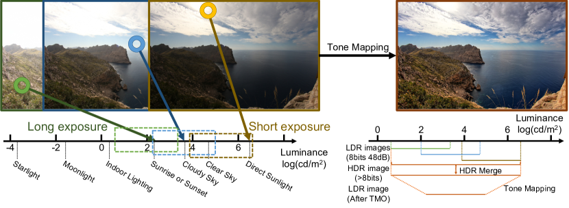
Figure 1.1: This figure illustrates how multiple exposure images are required to capture the wide ambient luminance levels that exists in our natural lighting environments. The HDR images produced from these multi-exposure images have higher bit-depths and a TMO is required to faithfully display it on a common display device (images from [68]).

Superior display quality is a dominant feature that has been driving the consumer electronics industry. Unlike the past, the growing demand for definitive viewing experience is not only limited to entertainment, gaming, and media industry but has been increasingly sought for applications in security and surveillance, automotive, medical, AR-VR, drones and robotics imaging systems. High Dynamic Range (HDR) imaging has come to become a compelling aspect of the new 4K/8K Ultra-high-definition (UHD) format [69]. Luminance and contrast, which are very important to the human eye, and our modern display systems have problems when dealing with visuals that may have details simultaneously both in sun, and in shadows. HDR imaging looks to solve these problems. This technique accounts for more realistically contrasted visuals by bringing out colors and detail in low-light areas so that visuals in shadow are not compressed, while not saturating the highlights. In other words, HDR can make the dark visuals deeper and the lights brighter, with more color shades with optimized contrast ratio of the display. However, this increase in amount of detail and extended color space comes at the price of higher data-width, thereby it requires more hardware/software resources to create, distribute and display HDR content.

Dynamic range of a digital images is defined as the ratio between the darkest and the brightest points captured from a scene [70]. It can be expressed in orders of magnitude (powers of ten), in stops (powers of two) or in decibels (db). From Fig1.1, we can notice that our eyes can see objects both in a dark night and in a sunny day, although the luminance level of a scene in sunlight is about $10^{6}cd/m^{2}$ and one with starlight is about $10^{-3}cd/m^{2}$ [71]. This means that our human visual system (HVS) is capable of adapting to wide lighting variations within range of nearly 10 orders of magnitude. From [70], it is learnt that HVS can easily adapt up to 5 orders of magnitude within the same scene. HDR imaging aims to increase the dynamic range recorded in a digital image from a given scene. Pixels in an HDR image are proportional to the radiance of the scene, dark and bright areas can be recorded within the same image. But one of the main limitations of our digital cameras is their inability in capturing and storing the HDR of the natural scenes. Which visually implies under and over exposure in bright and dark regions. Ordinary digital cameras produce images in a range lower than $1:1000cd/m^{2}$ [72]. There by most of the digital images are still Low Dynamic Range (LDR), with a data-width of 24 bits per pixel (in RGB format 8-bits per channel). Which translates to approximately 2 orders of magnitude while HDR images may have 80 orders dynamic range represented in floating point formats [70]. Common displays or printers represents only 8 bits per color channel (approximately $1:300cd/m^{2}$) [73], therefore HDR images need to be adapted (i.e., tone mapped) to 8 bits per color channel to display or print them in LDR devices. Figure 1.1 shows a tone mapped example of HDR image, notice that both bright and dark regions of the image are properly displayed.

There is a wide gap between the range of light that we can see & perceive and what a common digital camera can capture and display on a monitor respectively. Ordinary digital camera’s image sensors have limited capability for recording the entire illumination range in a natural scene. Also it is a challenge to determine good exposure values, especially in diverse scenes which have good large dark and bright areas. For example, taking a picture on a sunny day we have to chose whether to appropriately expose the bright sky and also account for the details in the shadow of the mountain slopes like in Fig 1.1. Modern digital cameras come with in-built auto-exposure algorithm to automatically set the ISO value, aperture and shutter speed corresponding to the given scene. However, a scene saturation (over-exposure) can occur if the scene is very brightly lit (direct sunlight) and sensor records the maximum allowed value, therefore details in bright areas are clamped to the maximum allowed value which is white. On the other hand, if the scene is poorly lighted and the light energy reaching the sensor is very low it results in under-exposed image. As stated earlier, we have to adapt the image so that we can match the dynamic range of HDR scene with the display device’s dynamic range, this process is widely known as tone mapping. Depending upon the dynamic range of the captured image tone mapping function can expand or compresses it in order to enhance the display quality [74]. The purpose of applying tone mapping on an image can be different and depends on the particular application. In some cases it may be to improve the aesthetics of the image, while for another application it might be to emphasize as many details as possible, or could be to maximize the image contrast [75]. However, the ultimate goal of tone mapping is to match the perception of tone mapped image with the real world perception [70]. A tone mapping operator (TMO) $f$ can be defined as a transformation function $f(I)$:

$$f(I):R^{w\times h\times c}\rightarrow D^{w\times h\times c}$$ (1.1)

Here, the tonemap function $f$ maps real world luminance $R$ to display luminance $D$ [71], and $I$ is an image with dimension $w\times h$ and $c$ is number of color bands which is $3$ for RGB image. Tone mapping has been an active area of research for the last two decades, resulting in the design and development of many hundreds of different tone mapping algorithms which can be broadly grouped in to global, local, frequency and segmentation operators [71].

Global TMOs, apply the same function to all pixels in the image. These mapping function treats every pixel of the image independently. These operators are computationally efficient, easy to implement and can be executed in real time. A local tone mapping function compresses a pixel value according to its luminance values and their neighboring pixels luminance values. Hence, for each pixel the computation is adjusted according to an average over a local neighborhood of pixels [70]. Frequency domain-based operators, like the local TMO preserve edges and local contrast by computing in the frequency domain instead of spatial [71, 76]. Segmentation operators divides input image into different uniform regions, and a global mapping operator is applied on each of these regions and finally these are merged to produce output image [77, 78]. HDR image pixels can have large disparity in intensities in small neighborhood thereby exhibiting artifacts in tone mapped images (particularly in local tonemap), like in Fig. 1.2. Therefore, various filters are required to suppress these artifacts and improve aesthetics of output images depending upon the targeted application.

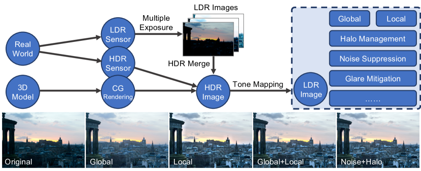
Figure 1.2: HDR imaging and tone mapping: Global tone mapping functions are good for capturing overall preview of the input image. Local tone mapping function by considering pixel neighborhood information for each input pixel, it can emphasize more local details. Additional filters are used to improve the subjective quality of tonemapped images (original image from [79]).

In literature, there have been many state of the art survey reports like [80, 81, 82, 83, 84, 85, 86]. These surveys mainly covered the software algorithms. The choice of a TMO operator is usually application driven, and in this report we study algorithms that have been optimized for hardware platforms like Application Specific Integrated Circuits (ASIC), Field Programmable Gate Arrays (FPGA) and dedicate Graphic Processing Unit (GPU). Strong demand for real-time embedded vision-based applications is on the rise in various domains like advanced automotive systems, medical imaging, robotics and Unmanned Aerial Vehicles (UAVs). The main building blocks for such vision-based systems are the image sensors, image processing algorithms and display monitors. For real-time applications with time constraints a hardware acceleration is necessary [87]. Also, embedded applications are energy and resource constrained there by simply porting software algorithms on a hardware platform may result in poor performance or even system failure. Therefore, image processing algorithms have to be optimized for hardware porting [88]. This redesign effort, which can exploit the hardware platform for optimal performance has produced many novel hardware tone mapping algorithms and architectures. In this survey, we report such hardware tone mapping algorithms and to the best of our knowledge there has been no such earlier survey. Following are our main contributions:

1. A comprehensive introduction to hardware TMOs and imaging pipeline.

2. Detailed survey of TMOs that have been implemented on an ASIC/FPGA and GPU platform.

3. Comparison of TMOs based on their hardware specification and performance.

4. Image quality assessment for hardware TMOs.

5. Demonstrate the link between hardware cost and output image quality.

6. Discussion on future perspectives for implementing machine-learning based TMOs on hardware.

The rest of paper is organized as follows: Section II covers HDR imaging. Section III presents a detailed survey of all hardware TMO algorithms. In section IV we will present the design issues and implementation TMO hardware techniques. We will also present figures of merit for these implementations, thus throwing light on design trade-offs. Image quality assessment is a very important performance metric, and in section V we list all the different metrics that are used in the current literature. While drawing our conclusions in section VI, we also present an account on the future research directions.

Chapter 2 High Dynamic Range Imaging

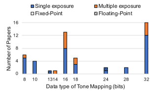
Figure 2.1: The histogram here shows the numbers of past tonemap operators input data-type. Most of the papers considered 32-bit HDR data.

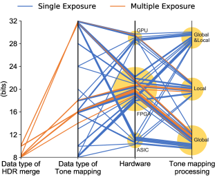
Figure 2.2: Data type based relationship between HDR images, TMO operators, and hardware platforms.

HDR images can be captured from real world scenes, rendered on computers by various computer graphics (CG) tools. In this paper we will focus mainly on methods of obtaining HDR images by using conventional cameras and special HDR sensors, which are useful for building real-time systems. For the CG methods there are well known books describing those methods [89, 90]. The gaming industry has been employing HDR rendering for very long time, they were used for rendering special visual effects like dazzling, slow dark-adaptation there by enhancing the immersive impression [91]. Today HDR imaging is used in many applications to enhance functionality of cinematography and photography [92], biomedical imaging (see DICOM standard [93]) [94], remote sensing [95] and many more computer vision applications [96].

Figure 2.1 shows the frequency of various data types used in all hardware tone mapping papers and whether HDR merge has been implemented in the hardware. Most works choose 16-bit or 32-bit HDR images for tone mapping, and only a few works choose other data types. Almost works proposed TMO on low-power embedded platforms are often implemented using HDR images with fixed-point arithmetic. Compare with floating-point arithmetic, fixed-point arithmetic has some advantages in embedded platforms such as low-power consumption, the small circuit size and high-speed computing [97, 98, 99]. On the other hand, due to floating-point arithmetic can save a huge range of luminance with small bit depth. Yadid-Pecht Orly et al. in [21, 38] proposed a FPGA implementation of tone mapping algorithm for HDR images with floating-point arithmetic.

Different researches implemented different TMO of HDR images with different data type on different hardware. Figure 2.2 shows how the work of hardware tone-mapping has been distributed and the relationship between data type, hardware and tone mapping processing.

2.1 HDR Merge

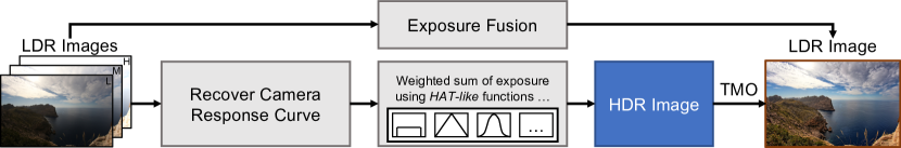
Figure 2.3: HDR Imaging: Using a camera response curve the full dynamic range of the scene is captured from a set of LDR images with different exposure times. Algorithms like Popadic et al’s can directly generate HDR-like images from bracketed images [35]. (images from [68]).

HDR images can also be composed by combining multiple LDR with different exposure time in a single HDR. Here, the exposure time which is also known as the shutter speed is the duration of time when the digital sensor inside the camera is permitted to capture light. The amount of light that reaches the film or image sensor is directly proportional to the exposure time. Therefore, a long exposure time image will have an overall greater luminance. It will detect smaller amount of light sources even in darker areas. But the picture might saturate in bright parts of the scene due to a too much of light for the sensor. On the other hand, a short exposure image will record bright parts of the scene but would not been able to register darker light sources. Exposure time values are often referred to as “stops”. A stop consists in doubling the exposure time (relative to a reference time). +1 stop is doubling, +2 stops is times 4, and -1 is halving the exposure time [100, 101]. So, there are many well known techniques to combine multiple images of varying exposures to compose a HDR image [102, 103, 104, 105].

For an LDR image, its dynamic range is bounded by the range of sensor i.e., a camera with 8 bits/pixel can only capture ratios up to 255:1. However, we can achieve a greater dynamic range using the same camera by combining multiple images which have been captured with different exposure time. Each of these LDR images will cover a different range of the luminance in the scene. This allows to have a greater resolution on the luminance captured . Images with a short exposure time will be adapted for capturing very bright parts of the scene but will fail to capture darker parts. Long exposure time images being the opposite. They will saturate in bright parts of the image. All intermediate images captured with various exposure time will help cover the whole range of luminance, this strategy is demonstrated in Fig. 2.3. The final composite image will have a greater dynamic range than it is achievable with a single shot by the camera.

2.2 HDR Image Sensor

There are broadly three different architectures that are used to design HDR image sensors (Fig 2.4). In the first group, by utilizing logarithmic response pixels or by employing likewise circuits to non-linearly extend the dynamic range as in [106, 107]. However, this non-linearity can cause severe problems when reconstructing images. The next group sensors like in [108, 109, 110] extend dynamic range by applying lateral overflow capacitors. But, this group of sensors would need to partially open a transfer gate so that the over-saturated charges can be collected by the overflow capacitor. Again, the threshold voltage of the transfer gates can have a large variation, thereby resulting in variations in saturation level. Also, this group of sensors is known to have higher dark current shot noise [111]. Mase et al., in [112] proposed a sensor design where they would use multiple exposure-time to expand the dynamic range. However, this method also has some issues; different integration time can cause discontinuities in SNR and also cause distortion in moving scenes. A new type of HDR image sensor was designed by Liu et al. [111] which used dual transfer gates. Their HDR image sensor is capable of capturing HDR scenes with low noise. The novelty of this design is it does not use the concept of transfer of threshold voltage and completes charge transfer in one operation.

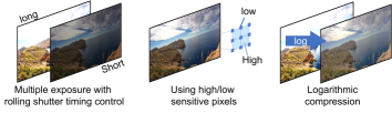
Figure 2.4: HDR image sensing methodologies (images from [68]).

Chapter 3 Tone Mapping Survey

3.1 Tone Mapping General Pipeline

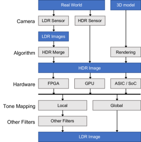
Figure 3.1: HDR-LDR Pipeline: HDR imaging, sensing, and tone mapping for display.

In the previous section 2 we discussed how to obtain/produce HDR content, and Fig 3.1 we show the broad HDR to LDR pipeline. This HDR content requires to be stored in a medium with a greater amount of bits/pixels than that of a single LDR image. It is necessary in order to achieve a greater dynamic range. Although HDR display systems do exist [73], and TVs with an extended dynamic range are currently available in the commercial market, but they are not as widespread due to their limitations in terms of dynamic range and color gamut. The process of tone mapping consists of reducing the dynamic range of the HDR image into an image that can be easily displayed on wide range of display devices which have limited dynamic range and color gamut.

This process can be highly non linear depending on the result expected. The LDR image after tone mapping will have less information than the original HDR image due to the reduction of information by the tone map function. But it is ready to be displayed, and the image has enough information by revealing details in both dark and bright parts according to the our perception. Tone mapping has been an important area of research as is evident from several surveys that have been published over the years [113, 92, 75, 114, 70]. Tone mapping function can be classified in to two broad groups based on the processing function they use.

• Global operators: The same mapping function is applied to all pixels through out image.

• Local operators: The mapping function applied to a pixel depends on its neighbors pixels.

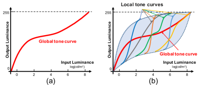
Figure 3.2: Deformation of tone mapping space. (a) Global Tone Mapping. (b) Global and Local Tone Mapping.

Figure 3.3: General block diagram for global tone mapping system for hardware implementation.

3.2 Global Tone Mapping Algorithms

Global tone mapping algorithms (also known as “tone reproduction curves”) are spatially invariant, that is they apply the same function to all pixels in the input image [115, 116, 117, 118, 119]. This results in one and only one output value for a particular input pixel value irrespective of the pixels in its neighborhood. Figure 3.3 shows a general pipeline which is useful for implementing a global tonemap function shown in Fig. 3.2 (a). As we can see, the tonemap pipeline first obtains the luminance image and from that it calculates global statistics (like $L_{max},L_{min},L_{average}$). In some algorithms these statistics are also calculated from previous frame based on a assumption that there is very little changes between successive frames when imaging at 30/60 frames per second [15, 16, 24].

In the pipeline next step is to realize a logarithmic or exponential like function to compute the tone mapped image. The hardware implementation of these functions are a challenge and a common approach is to approximate such functions, by maintaining an acceptable level of error in the realized implementation. As these functions are frequently required to be computed in many engineering and scientific applications many hardware friendly methods have been proposed in literature [120, 121, 122]. The final step in the pipeline after tonemap is to restore the color for displaying the output image. A detailed account for color correction technique is presented in section 3.4.

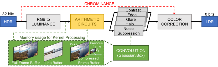
Figure 3.4: General block diagram for local tone mapping system for hardware implementation. For local calculation full frame buffer/line buffer or compressed frame buffer is required (images from [68]).

3.3 Local Tone Mapping Algorithms

Local tone mapping algorithms (also known as ’tone reproduction operators’) are spatially variant and apply different functions based on the neighborhood of the input pixel [123, 124, 125, 126, 127, 128, 129]. Therefore, one input pixel could result in different output values based on its position as illustrated in Fig. 3.2 (b). Local tone mapping algorithms are computationally more expensive and time consuming compared to global tone mapping algorithms [130]. We can describe the operation of a local tonemap algorithm using the block diagram shown in Fig 3.4. As was in the case of global tonemap, we initially obtain the luminance values for the input image. The color correction step is described in detail in section 3.4. The high computation cost for local tonemap operator is due to the local information calculation for which a full frame or a few lines of the input image has to be buffered as shown in the Fig 3.4. Some algorithms have also implemented compressed frame buffer (down-sampled images) to reduce the memory cost [12, 40]. To meet the real-time constraints, as a common approach previous frame is used to compute the local information for current frame.

Local tone mapping methods generally produce better quality images as they preserve details, which may not be the case when using global tone mapping methods [70]. However, one of the major drawbacks of local tone mapping algorithms are the creation of halo artifact among the high contrast edges and the graying out of the low-contrast areas [131, 132]. Therefore, local tonemap methods implement additional filters to suppress these image artifacts like halo and noise. Such filtering may require that the input image (of size $M\times N$) be convolved with a filter (of size $k\times r$). Benedetti et al. demonstrated a simple hardware sliding window convolution block, which can output one pixel every clock [133]. The latency associated with this sliding window method is calculated as:

$$T=Buffer_{depth}\times\left\lfloor\frac{KernelSize}{2}\right\rfloor+\left\lceil\frac{KernelSize}{2}\right\rceil$$ (3.1)

3.4 Color to Luminance

Image luminance are used for various applications such as printing, data compression, feature extraction and tone mapping. Thus, obtaining luminance is a very important step for TMOs. There are many well defined methods to obtain the luminance values from the color image. An easy method to obtain luminance is to compute it as a linear combination of the red, green, and blue component according to the RGB-to-XYZ conversion scheme. Here,

$$Y=0.2126R+0.7152G+0.0722B$$ (3.2)

is the luminance for the RGB image. Another effortless procedure is to use CIELab or YUV color spaces, and one could directly obtain luminance channel as the grayscale version of the color image. Because, they consider the luminance and color channel to be independent.

Tone mapping algorithms operate on the luminance channel which are obtained as described above. For a given HDR image luminance value is calculated and the chrominance values are buffered/stored as they are required later for restoring the color post tonemap. Different studies have used different luminance methods, which we have listed in table 4.1. Some studies have also used monochrome images [11, 15, 32, 45, 50], this approach can have certain advantages in terms of reduced memory, and fewer calculations. However, the application of monochrome images are limited.

After tone mapping, a common approach to restore the color is based on Schlick’s color ratios [116]:

$$C_{out}=\big{(}\frac{C_{in}}{L_{in}}\big{)}^{\gamma}L_{out}$$ (3.3)

In Eq. 3.3, $C_{in}$ represent the original RGB image, $L_{in}$ is the corresponding luminance value obtained by Eq. 3.2. If $L_{out}$ is the tone mapped luminance value then, we can compute three output chrominance values as in Eq. 3.3, where $\gamma$ is a color saturation factor for displaying color images, and its value is usually set between 0.4 and 0.6 [134].

Chapter 4 Tone Mapping Operators Implemented on Hardware Platform

Tone mapping HDR images/videos is a computationally challenging problem, and many hardware-based dedicate accelerators have been proposed for this purpose. In this section we will discuss those systems in detail. We have comprehensively listed these implementations in table 4.1, and summarized the number of these papers by year in Fig 4.1.

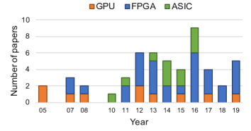
Figure 4.1: The number of TMO hardware implementation papers in the last 15 years.

Table 4.1: LIST OF TMO HARDWARE IMPLEMENTATIONS

TMO

Image

Image Quality

Previous work

Year

Hard- ware

Method

Reference

Kernel Sizeϵ

Channel

Lumi- nance

Data type (bit)

HDR Merge

PSNR (dB)

SSIM

Others

[1]

2005

GPU

G&Lγ

[126]

$49\times 49^{8\zeta}$

Color

24

No

RMS%=1.051

[2]

2005

GPU

Local

[126]δ

$61\times 61^{8\zeta}$

Color

XYZ

8to32κ

[135]

RMS%=0.245

[3]

2007

GPU

Local

[127]

$5\times 5^{2\zeta}$

Color

32

No

RMS%=0.038

[4]

2008

GPU

-

[119, 126, 125, 127, 124, 128, 129]

-

Color

32

No

[5]

2012

GPU

Local

[136]δ

$64\times 64$

Color

18

No

[6]

2012

GPU

G&Lγ

[137]

-

Color

XYZ

32

No

[7]

[18]

2013

GPU

G&L

-

$11\times 11$

Color

HSV

16

No

AMBE=108.09 DE=4.62 EME=11.306

[8]

2015

GPU

G&Lγ

-

$230\times 230$

Color

16

No

[9]

2017

GPU

Global

[138]δ

N/A

Color

32

No

TMQI=0.9236

[10]

[26]

2019

GPU

Local

[139]

multiscaleζ

Color

8

No

[11]

2007

FPGA

Local

[126]

$64\times 64^{9\zeta}$

Gray

$-^{\eta}$

28

No

34.94

[12]

2007

FPGA

G&Lγ

[140]

$5\times 5$

Color

HSV

10

No

[13]

2008

FPGA

G&Lγ

[141]

$61\times 61$

Color

YCbCr

8

No

[14]

2011

FPGA ASIPα

Global

[126]

N/A

Color

10.22λ

No

52.95

[16]

[15]

2012

FPGA

Global

[136]

N/A

Gray

10to16κ

[104]

[17]

2012

FPGA

Global

[126]

N/A

Color

$-^{\eta}$

18

No

[18]

2012

FPGA GPUβ

G&Lγ

[139, 142]

$7\times 7$

Color

HSV

16

No

17.35

[19]

2012

FPGA

Global

[143, 144, 145]

N/A

Color

8to14κ

[146, 147, 148]

[20]

[16]

2013

FPGA

Global

[136, 126]

N/A

Gray

10to32κ

[104]

[21]

2013

FPGA

G&Lγ

[149]

$3\times 3$

Color

20.12λ

No

54.27

0.9997

RMSE=0.932 SSE=0.233 R-squared=0.03549

[22]

[11]

2013

FPGA

Local

[134]

$3\times 3$

Gray

$-^{\theta}$

32

No

73.96

[23]

2013

FPGA

G&Lγ

[150]

$7\times 7$

Color

HSI

8

No

30

[24]

2014

FPGA

Global

[119]

N/A

Color

YUV

16

No

60.03

0.9995

[25]

2014

FPGA SoCβ

Local

[151]

$3\times 3$

Color

HSV

8

No

DE=5.01 EBCM=0.032 CEF=1.6

[26]

2015

FPGA

Local

[67]

$32\times 32^{3\zeta}$

Gray

HSV

8

No

43.37

0.9982

$\Delta E_{HS}$=0.0039

[27]

[20]

2016

FPGA

Global

[136, 126]

N/A

Gray

10to32κ

[104]

23.55

0.93

MSE=286.95 UQI=0.9

[28]

2016

FPGA

G&Lγ

[152, 153]

$5\times 5$

Color

20.12λ

No

57.27

0.9969

[29]

2016

FPGA

G&Lγ

-

$3\times 3$

Color

$16^{8}$ μ

No

55.87

0.9996

[30]

[22]

2016

FPGA

Local

[134]

$7\times 7$

Gray

28

No

GCC=0.75 DM%=0.88

[31]

[24]

2016

FPGA

Global

[119]

N/A

Color

YUV

8to16κ

[78]

103.61

[32]

2016

FPGA CPUα

Global

-

N/A

Color

HSV

16

No

[33]

2017

FPGA

Local

[125]

$9\times 9$

Color

$-^{\theta}$

8to16κ

[104]

39

[34]

2017

FPGA

Local

[154]

$11\times 11$

Color

YCbCr

8to18κ

[114]

[35]

2017

FPGA

Global

-

N/A

Color

8to8κ

Yes

[36]

[33]

2018

FPGA

Local

[125]

$9\times 9$

Color

$-^{\theta}$

10.8λ

[104, 155]

46.69

0.93

[37]

2018

FPGA

Local

-

$32\times 32$

Color

20.12λ

No

TMQI=0.9266

[38]

[29]

2019

FPGA

Global

-

N/A

Color

$10^{3}$ μ

No

TMQI=0.9111

[39]

2019

FPGA

Global

[156]

N/A

Color

16

No

81.47

0.9998

[40]

[28]

2019

FPGA

G&Lγ

[157, 158, 159]

$31\times 31$

Color

10

No

0.9696

TMQI=0.9360

[41]

2019

FPGA

Local

[160]

$29\times 29$

Color

5.13λ

No

[42]

2010

ASIC

G&Lγ

[126, 134]

$8\times 8$

Color

$-^{\iota}$

16.16λ

No

45/35

[43]

2011

SoC

Global

[161]

N/A

Gray

16

[162, 163, 164]

[44]

2013

Analog

Global

[165]

N/A

Color

HDR

No

[45]

2014

VSoC

Global

[70]

N/A

Gray

HDR

[135]

53.8

[46]

2014

Analog

Local

[119, 126]

-

Gray

16

No

[47]

2014

Analog

-

[116, 71, 119]

-

Gray

10

No

[48]

[47]

2015

Analog

Global

[126]

N/A

Gray

10

No

[49]

2015

Analog

Global

-

N/A

Gray

HDR

No

[50]

[51]

2016

Analog

Global

[126]

N/A

Gray

32

No

[52]

2016

Analog

G&Lγ

[126, 166]

$3\times 3$

Color

YUV

16

No

34.45

0.987

[53]

2016

Analog

Global

[70]

N/A

Gray

32

[167]

35

^αImplemented on two types hardware together ^βImplemented on two types hardware respectively
^γGlobal and local tone mapping operator ^δAn improvement of cited tone mapping operator
^ϵLocal luminance calculation kernel size ^ζ($i\times i^{k}$):$k$ scales Gaussian pyramid with a maximum size of $i\times i$
^η0.27R+0.67G+0.06B ^θ0.299R+0.587G+0.114B ^ι0.2654R +0.6704G +0.0642B
^κ($k$ to $i$):$k$bit LDR images into $i$bit HDR image by HDR merge
^λ($k.i$):$k$bits integer and $i$bits fraction ^μ($k^{i}$):$k$bits mantissa and $i$bits exponent

4.1 Design Bottlenecks: Software to Hardware Porting

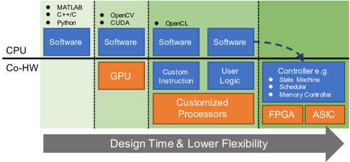
Figure 4.2: Choice of hardware platform for developing an algorithm mainly depends upon the application. Other important factors are design time and engineering costs.

Real-time image processing applications are bound timing constraints, i.e., for every pixel clock the processing pipeline should consume one pixel from the camera side and deliver one to the display side. Any missed pixel on either side would lead to loss of information or cause blanking display, this is known as the throughput constraint. When porting software algorithms to hardware an inherent design problem is that the SW code is developed on a general purpose CPU. Therefore, the algorithm is highly sequential, and it is useful to exploit the fast CPU. However, this is not the case on HW platform. For example, FPGAs are clocked at much lower frequencies and designers should exploit this parallelism to implement real-time systems. Another type of constraints that has to be met for real-time tone mapping system, is the pipeline latency. Here, latency implies how many clock cycles are required to process one input pixel to processed/tone-mapped pixel.

Memory bottleneck is crucial for implementing image processing algorithms on hardware. While HW platforms like FPGAs have highly parallel logic blocks and fast reconfigurable interconnects to speed up window (kernel) operations. The interface speed between the tonemap accelerator and the rest of the FPGA system is a bottleneck. Particularly, for image processing applications whose data bandwidth requirements are extremely high volume. The cost of moving data between off-chip memory and the accelerator can be detrimental and outweigh the benefits of implementing the FPGA system. Therefore, well thought out operation sequence that obeys raster order should be chosen, because other computation order would usually require the whole frame to be buffered. Like caching can reduce the memory bottlenecks on CPUs, streaming FIFO interfaces can reduce the amount of pixel accesses on FPGA hardware. Also, FPGAs are provided with BRAMs which can be read and written at the same time at every clock cycle, allowing one stream of values to be stored and one stream to be extracted in parallel.

Various technologies are available for implementing image/video processing algorithms. However, the main concerns of design implementation are cost, speed and power. The design methodology adopted for any hardware implementation depends on the application and time to market. The hardware-based implementation can be realized using any one of these hardware platforms: Application-Specific Integrated Circuits (ASIC), Field-Programmable Gate Arrays (FPGA), and Graphics Processing Units (GPU). Each have its own advantages and disadvantages, which we will briefly explain using Fig. 4.2. From this figure, we can notice that the choice of platform depends on various factors like: flexibility, design time and cost. A full custom ASIC design development will be very expensive due to increased manufacturing and design time, increased non-recurring engineering costs. Even though the ASIC design solution can be very efficient in terms of area and performance, it is only viable for proven designs that can be mass produced. GPUs and FPGA platforms have been preferred for many image processing applications and we will discuss more about them in the following sections 4.2 and 4.3. OpenCL-based is suitable for implementing algorithms on general-purpose computing on graphics processing units (GPGPU), and it has flavor similar to the proprietary CUDA language from NVIDIA. Recently, FPGA vendors are also supporting openCL development processes.

4.2 Graphics Processing Unit

GPUs came to prominence in 1990s to support more graphically realistic computer games, as it became hard to support good graphics and performance using CPUs only. GPUs are efficient and lot faster than a CPU in terms of floating point operations per second as they are specially developed for compute-intensive and highly parallel computations. As we know that image processing tasks are well-suited for parallel computing, and an average image consists of millions of individual pixels is a good case for GPU processing. Table 4.2 lists TMOs implemented on GPUs, and will be discussed in this section.

Table 4.2: GPU IMPLEMENTATIONS

	Hardware		Performance
	GPU	Technology (nm)	Frame Size (pixel)	Speed (FPS)	Throughput (Mpix/s)
[1]	Radeon 9800 Pro	150	$512\times 512$	5	1.3
[2]	GeForce 6800GT	130	$1024\times 768$	10	7.9
[3]	GeForce Go 6800	130	$2048\times 2048$	7	29.4
[4]	GeForce 8800 GTS	90	-	-	-
[18]	GeForce 7900 GTX	90	$640\times 480$	30	9.2
[5]	GeForce GT 550M$\times 2$	40	$1024\times 768$	2.8	2.2
[6]	GeForce 8800 GTX	90	$1002\times 666$	37	24.7
[7]	NVIDIA ION2	40	$640\times 480$	27	8.3
[8]	GeForce GTX 980	28	$1980\times 1080$	46.5	99.4
[9]	GeForce Titan Black	28	$2048\times 1536$	24	75.5
[10]	GeForce GTX 650 Ti	28	$4096\times 4096$	7.5	125.8

Goodnight et al. [1] proposed a tone mapping algorithm implementation [126] using programmable graphics hardware. This work also discussed, some applications of tone mapping for rendering. They cleanly map the tone mapping algorithm to the pixel processor, which allows an interactive application to achieve higher levels of realism by rendering. They also describe how the graphics hardware limits the effective compression of dynamic range and discuss modifications to the algorithm that could alleviate these problems.

Krawczyk et al. [2] propose a model include HDR image perception effects by local TMO [126] into a common computational framework and implemented on the Graphics Processing Unit. This work realized local tone mapping by constructing a Gaussian pyramid, implement the approach in graphics hardware unit as a stand-alone HDR processing module and achieve the real-time performance.

Roch et al. [3] propose a local tone mapping algorithm implementation [127] on graphics cards. They also present a modification of the luminance local adaptation computation, maintain the same quality appearance of the original TMO.

Zhao et al. [4] presented GPU implementations of two state-of-the-art TMOs with real-time performance. And include other six GPU-based TMOs [119, 126, 125, 127, 124, 128, 129], experimental evaluation is undertaken to explore which TMO is faster for hardware implementation.

Tian et al. [5] proposed a real-time hardware local implementation based on global TMO [136]. They proposed a algorithm of segmenting the image into $64\times 64$ independent rectangular blocks to sense local luminance. And a boundary and halo artifact elimination algorithm and a noise suppression algorithm are included in this work to improve the image quality of tone mapped image. Compare with CPU, GPU implementation can reduce the running time of a $768\times 1024$ pixels image from $1.477s$ to $0.358s$ in this work.

Akil et al. [6] presented a real-time GPU implementation of Irawan et al’s perceptual global tonemap operator [137]. The proposed system was implemented on an NVIDIA 8800 GTX GPU, they achieved real-time rendering for an HDR image dimension of $1002\times 666$ pixels by single program, multiple data (SPMD) parallel computing.

Ureña et al. propose a TMO and its real-time implementation in [7], this work is specially aimed as an aid system for visually impaired people who struggle to manage themselves in environments where illumination is not uniform or changes rapidly. The histogram adaptation of the luminance channel in HSV color space is used for the global tone mapping. And they propose a retina-like processing to enhance the local contrast. They achieved real-time (27 frame pre second) processing when working with $640\times 480$ RGB images on NVIDIA ION2.

Eilertsen et al. presented a GPU implementation for real-time noise aware-TMO that was developed in CUDA 6.5 [8]. The filter design utilizes base-detail layer decomposition for tone mapping and detail enhancement is achieved through a edge-stopping non-linear diffusion approximation. On the implementation side, this TMO pipeline can process a $1980\times 1080$ image with in 21.5 msec on a Nvidia GeForce GTX 980.

Khan et al. [9] present a tone mapping algorithm that uses histogram of luminance to construct a lookup table for tone mapping. This kind of global tone mapping is an improvement of histogram adaptation [138]. Compare with CPU, GPU implementation on NVIDIA GeForce Titan Black improve the speed from 0.09 FPS to 24 FPS for images of size $2048\times 1536$. The TMQI [66] average of this global TMO is 0.9236 in their database.

Tsai et al. presented a GPU accelerated image enhancement method [10], this is an improved method of their previous work [139]. Their CUDA parallel programmed implementation can process $4096\times 4096$ images at 64.9$\mu$s.

4.3 Field Programmable Gate Array

Table 4.3: FPGA IMPLEMENTATIONS

	Hardware				Cost							Performance
	Camera	Model	Tech- nology (nm)	Clock (MHz)	Latency (clock)	Power (mW)	Memory (bit)	Logic Elements	DSP	Registers	Others	Frame Size (pixel)	Speed (FPS)	Throu- ghput (Mpix/s)	pix/ clock
[11]	No	Stratix II	90	77.15	64	-	3,153,408	34,806	54	-	-	$1024\times 768$	60	47.2	0.61
[12]	No	Virtex II	150	1.3	-	-	20γ	17,280	-	890δ	F/F=1362η Multiplier=16	$125\times 86$	24	0.258	0.20
[13]	No	Stratix II GX	90	66.66	$2\times W\times H$ $+300$	-	2,609,151	49,763α	-	43,793	-	2.5M	25	50	0.75
[14]	No	Virtex 5	60	85	3,293,244 (Total)	-	3,932,160	5,806β	18	-	-	$1024\times 768$	25	19.7	0.23
[16]	EV76 C560	Virtex 5	60	94.733	65 clock /line	-	40γ	14,168β	4	8,132	-	$1280\times 1024$	30	39.3	0.41
[17]	No	Spartan 6	45	75	12288 @$163\mu s$	-	3γ	874β	17	1000ϵ	-	$1920\times 1080$	30	62.2	0.83
[18]	No	Spartan 3	90	40.25	-	900	39γ	30,086β	26	16,545ϵ	BufgMux=7 DCM=2	$640\times 480$	60	18.4	0.46
[19]	EyeTap	Spartan 6	45	78.125	-	-	100γ	-	-	-	-	-	30	-
[20]	EV76 C560	Virtex 6	40	125	136 clocks @1.2us	6	17γ	16,880β	-	20,192	-	$1280\times 1024$	60	78.6	0.63
[21]	No	Stratix II	90	114.9	nCols+12+7	-	68,046	8,546α	60	10,442	-	$1024\times 768$	126	99	0.86
		Cyclone III	65	116.5	nCols+12+7	250	86,046	12,154α	36	10,518	-
[22]	No	Stratix II	90	114.18	-	-	307,200	9,019	88	6,586	-	1M	100	100	0.88
[23]	No	Spartan 3	90	40	-	897	720,000	29,007β	26	11594	Slice=16545	1M	100	100	0.88
[24]	No	Virtex 5	65	214.27	-	-	8γ	4,536β	30	5,036	-	$1920\times 1080$	60	124.4	0.58
[25]	No	Cyclone IV	60	55.55	2Rows+18	-	-	1,784	-	-	Linebuff=4 F/F=510η	$2560\times 2048$	-	-	-
[26]	No	Cyclone II	90	170.24	-	-	98,594	838	10	680	CF=558ζ	$1920\times 1080$	80	165.9	0.97
		Stratix III	65	288.77	-	-	93,982	80	10	1,153	CF=418ζ	$1920\times 1080$	140	290.3	1.01
[27]	EV76 C560	Virtex 5	65	114	136 clocks @1.2us	-	30γ	6730β	-	-	F/F=6,378η	$1280\times 1024$	60	78.6	0.69
[28]	No	Cyclone III	65	100	83	674.25	87,176	93,989	28	26,004	CF=67,985ζ	$1024\times 768$	126	99	0.99
[29]	No	Cyclone III	65	100	2088	149.5	31,000	4,20	-	3,031	-	$1024\times 768$	126	99	0.99
[30]	No	Stratix II	90	114	-	-	614,440	9,019	-	-	-	$1280\times 720$	123	113.3	0.99
[31]	$-^{\theta}$	Virtex 5$\times$8	65	125	-	31.72W	3 γ	4,764β	54	2,489	-	$1024\times 256\times 8$	25	52.4	0.42
[33]	Python 2000	Zynq XC7Z020	28	200	-	-	2,160,000	29,850	-	-	-	$1920\times 1080$	96	199	1.00
[34]	Flare 2KSDI	Zynq XC7Z045	28	-	-	12W	47γ	24,700β	-	30,405	-	$1920\times 1080$	30	62	-
[35]	Yes	-	-	400	-	-	-	-	-	-	-	$2M$	33	66	0.17
[36]	Python 2000	Zynq XC7Z020	28	200	-	8Wκ	34γ	14,706β	38	20,316	-	$1920\times 1080$	96	199	1.00
[37]	No	Cyclone III	65	100	-	-	77,408	13,216	-	-	-	$1024\times 768$	126	99	0.99
[38]	Sensor	Cyclone III	65	100	-	-	107,408	15,471	-	-	-	$1024\times 768$	126	99	0.99
[39]	No	Virtex 7	28	150	-	819	-	-	-	-	-	$1024\times 768$	189	148.6	0.99
[40]	CX590	Kintex-7	28	162	-	453	9,738,000	9,799β	21	15,345	-	$1920\times 1080$	60	124	0.77
		Virtex 5	65	148	-	804	7,488,000	10,903β	22	12,794	-	$1920\times 1080$	48	100	0.84
[41]	No	Zynq 7000	28	148.5	@0.241ms	-	2,052,000	14,888β	-	21,627	-	$1920\times 1080$	60	124	0.84

^αAdaptive lookup table(ALUT) ^βLookup table(LUT) ^γBlock RAM(BRAM) ^δLogic cell ^ϵSlice
^ζCombinatorial function(CF) ^ηFlip-flop(F/F) ^θCell-phone cameras ($\times 16$) ^κInclude camera

FPGAs have been a popular platform for accelerating [168] and prototyping many image processing pipelines that include image sensors [169][170]. FPGAs are inherently parallel, and re-programmable which makes them an ideal choice for prototyping new algorithms. For pipelined designs, it is easy to model separate hardware for different functions on an FPGA. The large resources of logic gates, RAM blocks and very fast I/O rates and bidirectional data buses altogether make them an ideal choice for prototyping the full image processing pipeline including sensor interface. Usually, the initial algorithm is designed and simulated for functional verification in software (MATLAB) and then ported to FPGA. But, simply porting these algorithms directly to a hardware platform can lead to inefficient or failure of the implementation. It is necessary to redesign and optimize the algorithm for hardware implementation keeping in mind the underlying platform. In this section we will discuss, tone mapping algorithms and novel hardware architectures that have been implemented on FPGAs, which is listed in table 4.3.

In 2007 Hassan and Carletta reported a grayscale HDR tone mapping system implemented on an Altera Stratix II FPGA [11]. The proposed solution operates on a gray scale (luminance) pixel ($P$) which is obtained as $P=0.27R+0.67G+0.06B$. Their algorithm is based on Reinhard [126] and Fattal’s [134] local operators using approximation of the Gaussian pyramids. Their hardware implementation achieves 60 FPS for a $1024\times 768$ image for pixels with 28-bit depth. They reported their output image quality in terms of PSNR, and measured an average PSNR of 34.94 dB.

Durand and Dorsey in 2002 proposed a frequency domain based technique to tonemap HDR images [125]. This approach is similar to an earlier frequency domian filtering [171] in which low frequencies are attenuated more than higher frequencies. From [70] we can understand that in an HDR image base layer tends to be low frequency and HDR, whereas the detail layer is high frequency and LDR. In the bilateral filtering [125], a filtered output image is obtained by combining a compressed base layer with its detail layer. This approach has also been implemented on hardware. Marsi et al. [12], used a low-pass filter to split the input image in to a low frequency base layer and high frequency detail layer. They targeted an automotive driving assistance application using a Xilinx Virtex-II FPGA, and this system included temporal smoothing to prevent flickering and color shifting. They used a $\frac{1}{4}$ down-sampled previous frame, for temporal smoothing in order to reduce memory usage and the image was stored on FPGA. Their operator achieves 24 FPS for $125\times 86$ resolution.

Iakovidou et al., in proposed an Altera Stratix II GX FPGA is used for contrast enhancement on the images as they are received from the camera. Their algorithm is motivated by the attributes of the shunting center-surround cells of the human visual system. With a frame rate of 25 FPS, the FPGA calculates a histogram of each frame’s brightness level and transforms the image to have a stretched histogram at the output. Latency of their image processing pipeline is $2\times W\times H+300$ clocks, and the output image size can be up to 2.5 million pixels [13].

Lapray et al. [15, 16, 20, 27] in a series of publications presented several full imaging systems using a Virtex-5 FPGA-based processing core. Their HDR imaging pipeline uses a HDR monochrome image sensor to provide a 10-bit data output and making use of Debevec and Malik’s [104] fusion method to produces HDR video from multiple images. Using a special memory management unit [20], they can generate HDR images at the same frame rate as their camera output, which requires current frame and two previously captured frames. For HDR tone mapping they used global tonemap algorithms of Duean et al. [136] and Reinhard et al. [126]. Their FPGA accelerated tonemap system achieves 60 FPS at resolution of $1280\times 1024$ with a PSNR of 23.5 dB and a similarity index [59] of 0.93.

Kiser et al. [17] mainly proposes two improvements of real-time video tone mapping system. A pre-clamping operator which the light compensation algorithm based on reference white and reference black is used to adjust the brightness of underexposure and overexposed area. They present that the pre-clamped image effectively uses more of the available output dynamic range than no-pre-clamped image. Another improvement in this work is that the tone mapping parameter curve over time is smoothed for video flicker removal. They implemented the real-time 1080p tone mapped video system on Xilinx Spartan-6 LX150T with 12288 clock latency.

Mann et al. developed and prototyped a full HDR system using a Xilinx Spartan-6 FPGA for industrial application (arc welding). Their system receives images from two head-mounted cameras, which are stored in an external memory [19]. Using a set of pre-stored LUT values HDR scene is constructed from three LDR images of varying exposures. They calculate the radiance with a Comparametric Camera Response Function (CCRF). For final LDR display, an estimate of photoquantity is computed from the pixel values of sequential images, which is then combined with empirical values for adjusting brightness and contrast.

Ofili et al. [21] proposed a hardware implementation of an exponential tone mapping algorithm. The algorithm is based on global and local compression with automatic parameter selection. It uses the global information from a previous frame and $3\times 3$ convolution kernel to determine the local information. The output image quality has been objectively assessed using PSNR (Average = 54.27) and SSIM (0.9997) metric. Their algorithm was synthesized for both Altera Stratix II and Cyclone III FPGAs. However, this implementation is prone to halo artifacts [153].

Vytla et al. [22] developed hardware implementation of gradient domain HDR tone mapping using the Poisson equation solver inspired by Fattal’s operator [134]. This gradient domain compression algorithm is computationally very expensive, as it seeks to solve Poisson equation. The authors of [172] developed a local Fattal’s operator to solve the Poisson equation locally and repeatedly, thus making it parallelize-able there by executable in real-time. The modified Poisson solver uses only local information from pixel and its $3\times 3$ window neighbors, for computing a tone mapped pixel independent of Fattal’s operator on other pixel locations with in the window. An Altera Stratix II FPGA was used to implement this algorithm, and it outputs grayscale tone mapped images with an average PSNR of 73.96 dB.

The contrast enhancement technique proposed in [23] has targeted applications similar to [18] i.e., for people with poor vision. The algorithm operates in HSI color space and is based on histogram equalization. Here, an input image is divided into 35 blocks of 5 rows $\times$ 7 columns of size 100 $\times$ 100 pixels. The histogram is computed for 64 bins. The design is implemented on multiple platforms Spartan 3, Spartan 6 and Virtex 6. They report an operating frequency of 40 MHz (Spartan 3) to 69 MHz (Virtex 6). The FPGA implementation speed-up is 15 and 7.5 times compared to CPU and GPU implementations respectively.

Popovic et al. [24] used global TMO similar to Drago [119] operator. Drago’s operator uses a logarithmic mapping function, to calculate displayed luminance from the ratio of world luminance and its maximum. Logarithm calculations are known to be computationally expensive, so Popovic et al., used Taylor and Chebyshev polynomials to approximate logarithms [173]. Further, they designed a camera ring consisting of 18 independent cameras with different exposures to create panoramic HDR video [31].

Li et al. [26] presented a FPGA hardware implementation of a contrast-preserving image dynamic range compression algorithm. The FPGA implementation is a hardware-friendly approximation to the existing FDRCLCP algorithm [67], and used a line buffer instead of a frame buffer to process whole image data. These advantages significantly improved the throughput performance and reduced memory requirement of the system. This implementation required only a few hardware cost and achieved high performance (Fig. 5.2).

Ambalathankandy et al. [28] proposed a real-time hardware platform based on hybrid TMO [152]. This method uses local and global information from a previous frame to improve the overall contrast in the output image. Local operators are known to be prone to halo artifacts, to suppress halo in their tone mapped images they implemented a halo-reducing filter [153]. The proposed system was targeted for an Altera Cyclone III FPGA, processing images in the luminance channel and producing output images with an average PSNR = 57.27dB and SSIM = 0.9969.

In late 90’s mantissa-exponent representation were chosen to record digitized samples from the image sensor. Multiple sampling for exponentially increasing exposure times $T,2T,4T,...2^{k}T$ were coded with m bits. Each pixel sample were represented with m+k bits, where the exponents ranged between 0 to k and mantissa was m-bits. This representation extends the dynamic range by $2^{k}$ times, and provides m-bits resolution for each exponent range of illumination while incurring lower memory costs [174, 167]. Shahnovich et al. used this representation in their FPGA implementation [29]. Their TMO makes use of a simple logarithmic compression module for HDR images using this mantissa-exponent representation, they treat every input pixel to be 24 bit wide, where 16 bits is used for the mantissa and 8 bits for the exponent representation. Yang et al. [38] also considered the mantissa-exponent pixel to obtain a refined histogram which utilizes density and dispersion information to construct a piece-wise model for their tone mapping function. This FPGA implemented TMO system can process $1024\times 768$ images with 10 bits mantissa and 3-bits exponent.

Nosko et al. [33, 36] described a fast implementation of HDR merge processing by multiple exposure and a local TMO involving bilateral filtering [125]. This work also propose an application of de-ghosting method, which is dedicated for FPGA implementation. Compared with the use of Gaussian filter to detect local luminance, bilateral filter can preserves sharp edges, but also require more hardware cost. This work can output one pixel per clock on Zynq 7020 FPGA at 200 MHz.

Zemvcik et al. [34] presented a real-time HDR video acquisition and compression system built using FPGA that include captures multiple exposure HDR video [114], merges the standard range frames into the HDR frames and compresses the HDR video using TMO [154].

Popadic et al. [35] proposed an exposure fusion (Fig. 2.3) hardware implementation. This work implemented on FPGA inserted into standard industrial digital camera. The tone mapped images were obtained by using weighted summation of three images captured with different exposure times. The weight coefficient of each image was calculated according to the visibility threshold curve [175]. This work performs calculations on the global image level, and implements real-time (30ms/image) processing with 2M pixel images at 400 MHz.

Yang et al. implemented a segmentation-like TMO, here the input HDR image is divided into m$\times$n blocks [37]. The algorithm uses block-interpolated minimum and maximum values to determine the compression values. The Cyclone III FPGA implementation operates in a pixel-by-pixel fashion in the logarithmic domain processing 1024$\times$768 images operating at 100 MHz.

Liu et al. reported a retina-inspired [156] tone mapping algorithm by implementing horizontal and bipolar cell stages on a Xilinx Virtex 7 FPGA [39]. The design operated at 150 MHz consumed 819 mW power while processing a $1024\times 768$ image which corresponds to an energy efficiency of 544453 pixels/mW/s.

Ambalathankandy et al. presented a global and locally adaptive tone mapping algorithm and its FPGA implementation on a Xilinx Kintex 7 to process Full HD images [40]. They make use of a non-traditional white color space in their algorithm, a RGB color image can be transformed to this space as $W=\sqrt{\frac{R^{2}+G^{2}+B^{2}}{3}}$.Their tone mapping function, is based on local histogram equalization, controls global and local characteristics individually and can manage light/dark halos. By a weighted function, they demonstrate noise suppression in tone mapped images. To reduce memory access and latency, they use a downscaled previous frame (1/64).

Park et al. [41] presents the FPGA implementation of the efficient naturalness restoration algorithm [160]. The proposed FPGA design used small line buffers instead of frame buffers, applied a concept of approximate computing for the complex Gaussian filter, and designed a new nontrivial exponentiation operation to minimizes hardware resources while maintaining quality and performance. The design supports a throughput of 60 frames/s for a $1920\times 1080$ image on Zynq 7000 at 148.5MHz. In this paper, they normalized each resource of different types (LUT, register, block memory, and external memory)into memory bits to the user guide of each FPGA fabric [176, 177, 178]. And compared the normalized comparison metric with other FPGA tone mapping implementations which are implemented on different models.

4.4 Application Specific Integrated Circuits

As we saw earlier, building full custom solutions on ASIC is expensive and time consuming. However, there may be applications with specific demands on power consumption, size of the hardware or some security aspects that may need specific ASIC implementations. ASIC is useful for building dedicated hardware which can be integrated on a single chip with sensor. They can clock at very high speed, and be faster than a commonly used camera. There by, making it possible to process the data and be sent out for further actionable controls. In table 4.4 we have listed TMO algorithms realized on ASIC platform, and details of which follows next.

Table 4.4: ASIC IMPLEMENTATIONS

	Hardware					Cost			Performance
	CMOS Sensor	Foundry	Technology ($\mu m$)	Monolithic	Clock (MHz)	Area(mm2)	Power (mW)	Gate Counts	Frame Size (pixel)	Speed (FPS)	Throughput (Mpix/s)	pix/ clock
[42]	No	TSMC	0.13	No	100	$2.85\times 2.85$(Core)/ $3.74\times 3.74$(bond)	177.1478	769,620	$1024\times 768$	60	47.2	0.47
[43]	Yes	-	-	No	-	$1.98\times 3.88$(Chip)	-	-	$64\times 64$	-	-	-
[44]	No	AMS	0.35	No	-	-	-	-	$256\times 256$	-	-	-
[25]	No	TSMC	0.13	No	200	$1.835\times 1.835$ (Core)	-	15,742	$2560\times 2048$	37	194	0.97
[45]	Yes (151dB)	AMS	0.35	Yes	-	$7.33\times 6.78$(Core)	111.2	-	$180\times 148$	1205	32.1	-
[46]	Yes (120dB)	Lfoundry	0.15	in-pixel	-	-	-	-	-	-	-	-
[48]	No	AMS	0.35	in-pixel	-	-	-	-	-	-	-	-
[49]	Yes (102dB)	-	-	No	-	-	-	-	-	-	-	-
[50]	Yes	-	0.15	in-pixel	52	-	54.72	-	$1024\times 768$	66	51.9	1
[52]	No	TSMC	0.35	Yes	-	0.039	41	-	-	-	-	-
[53]	Yes (CIS)	-	-	Yes	-	-	-	-	$512\times 512$	-	-	-

A $64\times 64$ pixels image sensor using 5 transistors APS per pixel with adaptive integration method is proposed by Punchihewa et al. [43]. Their They developed a tone compression algorithm that is based on improved local histograms and using differential-luminance histograms. The proposed system was tested using a 16 bit image raw data.

Sicard et al. [44] described an analog model of the Gamma correction method proposed by Meylan et al. [165] for local tone mapping. Sicard’s method improves upon digital normalization of the pixel output and this is in line with the Michaelis Menten law, however this study reports few preliminary results only.

Shiau et al. developed a transformation domain-based method to estimates illumination by a bi-dimensional empirical mode decomposition [25]. They adjusted the image contrast by gamma correction there by avoiding over-enhancement in the output image. The algorithm was implemented on multiple hardware platforms, SYNOPSYS DV was used to synthesize the design with TSMC 0.13$\mu$m technology. The synthesized design core size was 3.367$mm^{2}$ with a gate count of 11.6K and with a clock period of 5 ns and can achieve a processing rate of 200 Mpixels/s. The design implemented on FPGA consumed 1,784 logic elements and operated with a clock at 55 MHz.

Vargas-Sierra et al. [45] developed a proof-of-concept HDR CMOS image sensor that implemented a global tonemap compression during image capture operation. The system has been conceived as a complete Vision System-on-Chip (VSoC) with a core area of $7.33mm\times 6.78mm$ was fabricated on $0.35\mu m$ opto-flavored technology. This system achieved video rates for QCIF resolution images with 25 bits/pixel and tonemap them to 7 bit/pixel for display. But, an off-chip processing is required to compute image histogram before the final display [179].

Gouevia et al. in [46] present a new programmable pixel based on variable integration time. In this proof-of-concept, the integration time is a function of the light intensity and is an user controllable signal. Using this programmable pixel, they try to simulate the monotonic non-linear response of tonemap functions. They studied three different operators [126, 70, 119] and tested the implementation output for various test images [83, 180].

Mughal et al. in [48] reported a new pixel with inbuilt TMO, this operator was based on, the Reinhard’s photographic TMO [126]. The performance of pixel circuits are limited by the fixed pattern noise(FPN) which is mainly due to the variations between the responses of individual pixels within an array of pixels. Mughal et al. devise a calibration technique to to correct the fixed pattern noise in pixels which can produce a tone mapped response.

Fernandez et al. [49] designed a vision sensor with dual photodiode pixel, of these two photodiodes large one enabled them to capture high sensitivity and the small low sensitivity in the same exposure. Also, the large photodiode sensed the pixel value and the small photodiode achieved a tunable balance between local and global adaptation. By taking inspiration from earlier work [45], a global operator for HDR tone-mapping compression based on an online evaluation of the image histogram is implemented in OpenCV. The proposed system fabricated in 0.18$\mu$m CMOS technology can capture an image with dynamic range up to 102 dB.

Shi et al. [50] modeled Reinhard’s [126] photographic tone reproduction operator in analog domain using Verilog-A. Their global tonemap operator achieves 60fps for $1024\times 768$ monochrome images while consuming 54.27 mW power. They also demonstarted the usefulness of this work to improve the dynamic range of CT images that are affected by overexposure artifacts [51].

Chen et al. [52] designed an analog current-mode joint global and local tonemap operator based on [149]. From simulations they report, their TSMC CMOSP35 implementation consumed 41 mW power from a 3.3V supply and it requires 1$\mu s$ processing time per pixel.

Compressive sensing (CS) based HDR imaging was proposed by Guicquero et al. [53]. Their method utilizes cellular automaton for a scalable and low-complexity column based compressive sensing. They describe an imager architecture for $512\times 512$ pixel and a dedicated global tonemap reconstruction algorithm. The algorithm iteratively evaluates image contrast. To emphasize low-light details and to suppress noise the iterative tonemap operation flattens out the histogram.

4.5 Customized Processors and Other Hardware Platforms

Application Specific Instruction set Processors (ASIP) has lately emerged as an attractive platform to implement signal processing algorithms [181]. ASIPs are highly customizable, and embedded with domain-specific hardware accelerators, and these hardware accelerators are strongly coupled with the processor pipeline and are easily accessed by custom instructions. An ASIP can be systematically customized for implementing a specific application due to the availability of custom instructions, availability of optimized domain-specific blocks, and other parameterizable options [182]. ASIPs have been used for real-time Retinex-like image and video enhancement applications [183][184] and global tone mapping [14].

Saponara et al., in [183] presented a programmable class of Retinex-like filters, based on the separation of the illumination and reflectance components. The dynamic range of an input image is modified by applying a non linear function to compress the illumination layer and enhancing the details in the reflectance layer. They proposed 42 new ASIP instruction set which perform: color conversion, nonlinear transformations, arithmetic computations, memory accesses, initialization, and loop control. The final design was synthesized using Synopsys in $0.18\mu m$ 1.8V CMOS standard cells technology. Their system could process a $256\times 256$ video at up to 29 fps.

Vakili et al., in [14] proposed an implementation of Reinhard’s global tone mapping algorithm [126] on a customized LTRISC, which is a 32-bit RISC-like processor model provided with Synopsys Processor Designer. Using the LISA ADL, they developed three instructions to based on a specific low cost technique presented in [185] to calculate (i) luminance, (ii) logarithm and (iii) maximum luminance. They manually determined word length for all the intermediate variables. The system was synthesized for a Xilinx Virtex-5 FPGA and achieves 25 FPS for image size of $256\times 192$ pixels using a clock frequency of 85 MHz. The system outputs image with an average PSNR of 50dB.

ASIPs have comparatively better energy and area efficiencies than the digital signal processors (DSP) and general purpose processors (GPP) [186], while it does offer the flexibility and programmability for algorithm re-design/upgrades and bug-fixes. However, this programmability feature comes at a price of increased area (loop control, registers, etc.), when compared to ASICs. Development of an ASIP system is laborious, as is evident from the 2 man-months effort spent for Architecture Description Language (ADL) design in [183], further the system development not only involves design and verification of ASIP architecture but also the construction of the associated software tools such as assembler, compiler, debugger and instruction set simulator [182].

Chiu et al. [42] developed a tone-mapping processor based on an ARM core with an application-specific integrated circuit (ASIC). Their processor includes a modified global photographic tone mapping and a block-based gradient domain compression, based on algorithms proposed by Reinhard et al. [126] and Fattal et al. [134], respectively. The processor can run at a 100 MHz clock rate and can compress $1024\times 768$ HDR images at 60 fps. However, this approach does not offer the flexibility like others [183][184][14] since some critical modules are implemented on an ASIC core that occupies $8.1mm^{2}$ of physical area in $0.13\mu m$ TSMC technology.

Ureña et al. [18] implemented their own optimized tone mapping algorithm. Their algorithm operates in HSV color space and performs histogram equalization of the brightness (V) channel. They also perform local detail enhancement by a $7\times 7$ window convolution. The output brightness is a simple combination of the convolution output and histogram equalization. Their algorithm also included a glare mitigation filter, as they intended to develop this system for a low power battery operated device for visually impaired people. They prototyped it on two different platforms, one on a Xilinx Spartan III FPGA and a Nvidia ION2 GPU. Their proposed implementations delivered real-time performances of 30 FPS and 60 FPS on GPU and FPGA respectively for $640\times 480$ image resolution with an average PSNR measure of 17.35 dB. In their subsequent work they implemented a filter to attenuate glares in images, because people with poor vision have difficulties in adapting to illumination changes [7].

Narashima and Batur [187] presented a real-time tone mapping algorithm implemented in software using Texas Instrument Davinci media processor [188]. In their implementation, a luminance image is divided into overlapping blocks and a block mean pixel value is computed for each of the blocks. Several local tonemap functions are used to adapt each of the sub-blocks. A limitation of this algorithm is the choice of the block size and amount of overlap which may have to be determined empirically, there by limiting its practical application as it can significantly affect its quality and performance.

Chapter 5 Quantitative Comparison

5.1 Hardware

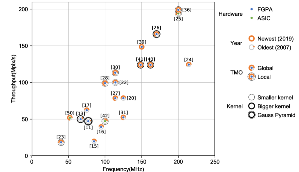
Figure 5.1: TMOs Performance Measurement: Throughput versus operating frequency is an important measure for real-time performance.

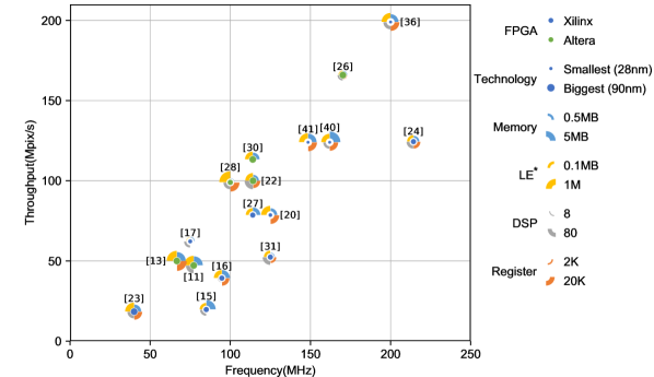
Figure 5.2: Throughput versus Hardware Cost: TMO cost is evaluated in terms of memory, DSP, logic elements and registers. Global TMOs are usually light-weight in comparison to local TMOs.

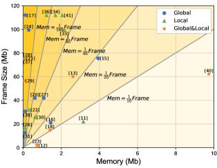
Figure 5.3: Memory Cost: Plot illustrates memory cost of tone mapping algorithms versus output images. Typically global TMOs have lower memory requirements than local TMos.

As stated earlier, one of the main objective of our survey is to determine the quality of various TMOs. In Fig 5.13 we present ASIC and FPGA implementations grouped on a map. In the map a blue dot imply FPGA implementation, and green one is ASIC. The positions on this map highlights these implementations according to their frequency and throughput. We computed throughput as shown in Eq. 5.1

$$Thoughput=Height_{Image}\times Width_{Image}\times FPS$$ (5.1)

Frequency and throughput are very important parameters, as it allows us to predict the algorithm’s effectiveness for processing HDR images of wide-ranging resolutions. In other words, more throughput per cycle implies that the algorithm is faster, and is well optimized. The orange circle in Fig 5.1 represents the year of publication. A paper which has full circle (in orange color) means chronologically newer paper, and arguably this paper would have improved design architecture than those in previous papers, thereby, realizing some design optimization. The black circle gives information of tone mapping. The width of black circle corresponds to the size of kernel that is used to calculate the local luminance. Works based on global TMO are without black circle because they do not use any local statistics. With respect to local operators, some of those works have calculated local luminance by using Gauss Pyramid, such implementations are represented as double black circles and their performances are also included in Fig 5.1. Figure 5.2 illustrates the hardware cost of FPGA tone mapping implementations. Like in Fig 5.1 the location of each point is grouped with respect to the system throughput and frequency, so that same position corresponds to same paper in both figures of merit. The color of center circle of each point informs about the FPGA manufacturer (ALTERA/XILINX) that were used in research. And the size corresponds to the FPGA’s manufactured technology. Smaller size represent that they use newer 22nm technology.

To compare the TMO algorithms implemented using different FPGA families, we follow the hardware normalization strategy proposed by Park et al. [41]. For algorithms implemented on Xilinx Virtex-4, each LUT and register consumed can be substituted with 16-bit memory. For systems that are implemented on a Virtex-7/Zynq7000, and those seven series FPGA’s LUT and registers are equalized with 32-bit memory. For Altera Cyclone III based systems, according to an article analyzing the difference between the two FPGA fabrics [178], one unit of the logic element used in Cyclone III is 1.3 times larger than one unit of LUT used in Virtex-4, so the resource utilization is converted into the estimated amount of LUTs of Virtex-4. This method of normalizing hardware resources between different FPGA fabric usages for comparison has also been adopted by Choi et al. [189]. The size of the circle sector area is proportional to the hardware cost. Different colors represent different type hardware. By studying Fig 5.1 we can see that recent works [25, 36, 40] have high throughput.With streaming applications like tone mapping which continuously process data, throughput is the most interesting design aspect as it will define the performance of the tone mapping application. More throughput means that more data can be processed in the same instant of time. To improve the performance of slower algorithms, one of the most effective ways to is by adding extra pipeline stages. FPGA designs have a synchronous nature consisting of delay elements and logic, which means that it highly benefits from extra pipeline stages.

Another interesting design aspect is the memory cost, Fig 5.3 shows the relationship between TMO HW implementation memory and output frame size. Frame size is computed as shown in Eq. 5.2. From the Fig .5.3 we can observe that, as expected global TMOs require less memory than local TMOs. In the Fig 5.3, we have grouped the algorithms based on the performance as which of these implementations are better designed to reduce memory cost. Recent local and global TMO works [34, 36, 41] report low memory usage by highly optimizing their designs. For example, Park et al., designed a frame-less TMO system, and only used a small line buffer[41]. They further optimized their design by building an approximate convolution block of a $29\times 29$ Gaussian filter. A conventional 2-D filtering scheme would have required $29\times 29$ convolutional operations between a pixel and its coefficient. They implemented it by using two 1-D separable filters operating vertically and horizontally, thereby reducing the number of operations to $29\times 1$ plus few additional adders.

$$Frame_{Size}=Height_{Image}\times Width_{Image}\times Datawidth$$ (5.2)

5.2 Data Conversion for Optimal Hardware Specification

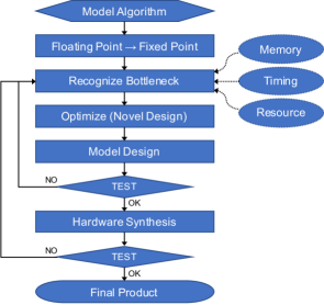
Figure 5.4: Flowchart listing common approach to adapt a software algorithm to a hardware platform.

The cost of modern electronic devices is usually measured in terms of silicon area (chip footprint), power consumption and algorithm/application execution time. Engineer’s strive hard to keep these three factors to a minimum while attaining all the system objectives. Balancing these goals are extremely challenging in nature, and usually a delicate trade-off between system performance and cost has to be planned in advance. Therefore, it is very important to make careful decisions in every design step to ensure the best possible performance of the entire system. Direct porting of a software tone mapping algorithm to any hardware platform will be inefficient and even may lead to system failures. The various stages of the design flow of a digital signal processing application are described in Fig 5.4. As a first step the algorithm is designed, simulated and thoroughly tested using DSP software tools like MATLAB/Simulink (Mathworks Inc) or others like Scilab etc. These software implementations achieve high degree accuracy as the algorithms are described with floating-point arithmetic. However, the choice of arithmetic operators used to implement the algorithms, has a decisive impact on the cost-performance trade-off. On a hardware platform fixed-point arithmetic operators are ideal choice as they require low area (footprint), low power, and have low latency [190].

But, the floating-point to fixed-point conversion process is an optimization problem which derives the data word-length [191]. This adaptation has to be carefully crafted as this leads to a trade-off between cost and performance. Reducing the data-width leads to significant quality degradation and therefore appropriate assessment is required to various stages to ensure acceptable performance. Also, this conversion process is not straightforward and may require significant design effort. But it is encouraging to note that there are automatic floating-point to fixed-point conversion tool which can significantly speed-up this process [192]. Next step in the design cycle is to determine the data-width for integer and the fractional part. It is absolutely necessary to establish this step by performing detailed numerical analysis as this will effect the overall performance due to accuracy of the algorithm. The integer part determines the dynamic range of the data and fractional part determines the numerical accuracy. The integer part determines the minimum and maximum values and, the designer has to accurately determine the number of bits required to represent the range depending upon the application thereby avoiding any overflows.

Recently, some High Level Synthesis tools (HLS) like Intel HLS, Cadence Stratus etc. have emerged, which can directly generate register transfer level (RTL) implementations from a C/C++ fixed-point specification of the algorithms [193, 194, 195, 196]. Use of these tools can speed-up the re-design effort, but the designs may not be fully optimized. Other issues that affect the direct adoption of fixed-point arithmetic from the floating-point designs using HLS:

• Bit growth: When performing arithmetic operations like addition and multiplication, designer has to maintain adequate width on datapath. Over-constrained designs can lead to loss of accuracy and relaxed approach could lead to waste of resources.

• Complex functions: When performing various complex mathematical functions (transcendental) in floating-point algorithm (for example in MATLAB/C/C++) is precisely defined. However, accurate equivalent hardware micro-architectures may not be available.

5.3 Image Quality Assessment

Table 5.1: Image Quality Metrics

	Image Quality Metrics		Ideal Value	Reference
	SSIM	Structural Similarity Index	1	[59]
	TMQI	Tone Mapped Image Quality Index	1	[66]
	PSNR	Peak Signal to Noise Ratio	higher is better	$20log_{10}(\frac{MAX}{RMSE})^{\ddagger}$
	RMSE	Root Mean Square Error	0	$\sqrt{MSE}$
	MSE	Mean Square Error	0	$\frac{SSE}{mn}$
	SSE	Error Sum of Squares	0	$\sum\limits_{i=0}^{m-1}\sum\limits_{j=0}^{n-1}[I_{ij}-G_{ij}]^{2}$
	RMS%	Root Mean Square Percentage	0	$\frac{1}{mn}\sum\limits_{i=0}^{m-1}\sum\limits_{j=0}^{n-1}[\frac{I_{ij}-G_{ij}}{I_{ij}}]^{2}$
	R-squared	Coefficient of Determination	1	[64, 56]
	DE	Discrete Entropy	higher is better	[54]
	EBCM	Edge-Based Contrast Measure	higher is better	[55]
	CEF	Color Enhancement Factor	higher is better	[63]
	$\Delta E_{HS}$	Color Similarity	0	[67]
	UQI	Universal Quality Index	1	[57]
	AMBE	Absolute Mean Brightness Error	0	[58, 65]
	EME	Enhancement Measure	higher is better	[61, 62]
	GCC	Global Contrast Change	higher is better	[60]
	DM%	Detail Maintenance Percentage	higher is better	[30]

• $MAX$ is the maximum possible pixel value of the image.

Image Quality Assessment (IQA) is plays vital role at many levels of the design cycle, and an early assessment is inevitable to prove the usefulness of the algorithm. subjective user study is the most reliable means to measure image quality. However, it is not always feasible for practical reasons. During the hardware development stages, objective image quality metrics are used to evaluate the system performance and analyze if there is more room for optimization. IQA studies has been actively carried out and there are several quality metrics in literature [197, 198, 199]. These IQA methods try to accurately predict the subjective preferences of a common human user by surveying the perceived quality of visual data presented to the user. These user studies are grouped as full-reference and no-reference IQA methods depending upon the availability of ideal reference images, with which the images (here tone mapped images) will be compared.

For algorithms implemented on hardware, IQA is measured in terms of image distortion which is caused by the approximations due to floating-point to fixed-point translation. From our survey we observe that in literature PSNR is a preferred metric to measure the pixel value distortion between software and hardware tone mapped images. Other metrics also have been used and they are all listed in table 5.1.

As stated earlier, among them the most commonly used metrics are peak signal to noise ratio (PSNR), structural similarity (SSIM) index and tone mapped image quality index (TMQI).

PSNR is a well-known quality metric used to evaluate the image quality by the mean-square error (MSE). Similar to PSNR, some traditional metrics based on square error were also been used for image quality assessment in tone mapping hardware implementation, such as root mean square error (RMSE), mean square error (MSE), error sum of squares (SSE), root mean square percentage (RMS%), R-squared and so on. The PSNR value approaches infinity as the MSE approaches zero, this shows that a higher PSNR value provides a higher image quality. But the PSNR perform badly in discriminating structural content in images since various types of degradations applied to the same image can yield the same value of the MSE [200, 201].

Therefore, some more elaborate methods attempt to incorporate structural information in IQA. Wang et al. [59] proposed SSIM based on human visual perception for measuring the similarity between two images, and Yeganeh et al. [66] proposed an objective quality assessment algorithm for TMO and named it as TMQI which is based on SSIM and naturalness. In TMO hardware implementation works, SSIM is used for pixel-to-pixel calculating the similarity between tone mapped images by software operator and hardware implementation. During hardware implementation, there have some losses due to approximate calculations, and SSIM is used to measure these losses. When SSIM is close to 1, it indicates that losses in hardware implementation is small. And TMQI is used for measure the tone mapped quality from HDR images to LDR images which were processed by hardware.

Some previous works have used some special metrics for image quality assessment. Such as, discrete entropy (DE)[54] for measuring the degree of details in images, edge-based contrast measure (EBCM)[55] for evaluating the contrast of images, color enhancement factor (CEF)[63] for measuring colorfulness, $\Delta E_{HS}$ for color similarity, universal quality index (UQI)[57] for the similarity between two images, absolute mean brightness error (AMBE)[58, 65] for the preservation of the original image brightness, enhancement measure[61, 62] and global contrast change[60] for contrast. Some works also present their image quality metrics, like detail maintenance percentage [30].

5.4 Hardware Specification versus Image Quality

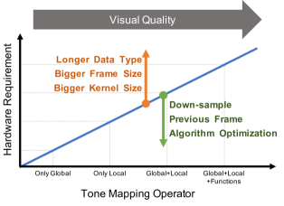
Figure 5.5: Trade-off: Visual quality versus hardware specification.

Every image processing application seeks to achieve good output image quality, and TMOs are no different. Local TMO’s are known to produce better images than global TMOs as they can reproduce both global and local contrast [71]. However, local TMOs are computationally more expensive than global TMOs and also may generate artifacts like halos around edges and amplify noise [125]. Therefore, additional functions are required along with local TMOs to reduce such artifacts. These local operations must be repeated over large amounts of data and usually demand substantial computational effort as shown in Fig .5.5, the visual quality does improve but at the expense of additional hardware. At the same time, depending on the data-type, image and kernel size will also increase the cost. As shown in Fig .5.5, cost can be reduced by applying techniques like operating the algorithm with previous frame/down-sampled images or employing other optimization techniques that can reduce computation or memory operations.

As stated earlier, local contrast enhancement algorithms risk boosting noise. Many algorithm designers proposed various techniques to suppress noise. Eilertsen et al. presented a novel noise control with display-adaptivity to produce high contrast and detailed video given the display limitations [8]. Li et al. presented a new logarithmic CMOS sensor and a histogram-based tonemap operator which is derived from cumulative distribution function with an objective to suppress noise in the tone mapped image [32].

Ambalathankandy et al. in [28] implemented a halo reducing filter based on a Gaussian-like filter [153]. In their TMO operator, halos were created around small bright features due to strong attenuation of neighboring pixels due to convolution operation with low-pass filtering. The hardware scheme for reducing such halos resulted in a very expensive implementation.

Nosko et al. [36] proposed a ghost removal algorithm which significantly improves perceived quality of HDR image. This method is based on an earlier work of Grosch [155], and requires only simple arithmetic operations and thus it is suitable for implementation on FPGA. The ghost detection step is implemented before the HDR merging step. By constructing the ghostmap, marked pixel positions are treated differently from unmarked ones during the HDR merging.

Recently, Ambalathankandy et al. [40] designed and implemented a LHE-based TMO that requires only one box filtering with a wide kernel. Their TMO algorithm uses two curves, one corresponding to the edge region and the other for gradation. As noises in gradation part are much more noticeable than in the edge and texture part. They use an alpha blending function to suppress noise in gradation region, and they include a halo control mechanism to manage light/dark halos individually using a simple weighting function on the bin-reduced histogram.

5.5 Preferred Platform for Accelerating TMOs

From Fig 4.1 we can observe that from early days FPGAs have been preferred platform for realizing real-time tone mapping applications. The main reasons are FPGAs popularity are:

• High Performance: The underlying FPGA fabric supports development of very deep pipeline architectures, with scope for wide parallel computational elements. This flexibility permits the designer to easily develop complex functionalities with strict timing constraints. Current generation of FPGAs can accelerate whole algorithm while processing full HD images or higher resolution images.

• Re-programmability: This is one of the most attractive feature of FPGAs. A designer can iterate his design to make sure that he can tune his design to meet specific needs of targeted application without incurring additional cost.

• Low Cost: The cost of developing a design on FPGA is comparatively cheaper, as many vendors provide customizable IP’s and reference designs which can speed-up the development process.

• Development Tools: Good support is available in the form of full development suite. Altera and Xilinx have streamlined development software for design and verification.

• Flexibility for ASIC migration: FPGA proven design can be ported to structured ASICs which are available from many vendors, there by giving developers a faster route to market their products[202, 203, 204].

Chapter 6 Future Perspectives and Conclusion

Currently machine learning-based (ML) methods have become a very important tool to solve many computer vision tasks like image classification, face detection, and video analysis. As a future perspective we would like to leverage its potential by accelerating ML-based TMOs using hardware platforms. In this section we will explore the challenges and opportunities that we will encounter for such systems. Usually image processing tasks would require multiple convolution with fully connected layers, which are exorbitantly computationally intensive (for example, the operations in CNNs are over billion operations [205]). Realizing such systems on resource constrained embedded systems would require very novel architectures and algorithms. FPGAs have been preferred platform for realizing CNN hardware accelerators for their following well-known features: re-programmability, low-power design features, and quick design time [206, 207].

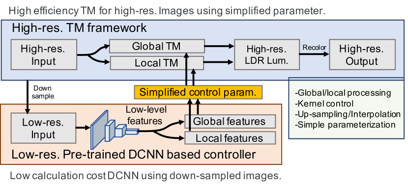
Figure 6.1: Future Perspective: Block diagram for a plausible machine learning-based TMO implementation on hardware.

Using Fig. 6.1 we demonstrate how Gharbi et al.’s HDR-Net like architectures are ideal baselines for realizing TMOs with DNN on hardware [208]. We find such designs are more hardware friendly because of the following features. First, the bilateral grid inspired architecture represents local tone-control as simple parametrized luminance grid in the space. Thus, the HDR-Net like high throughput design can approximate a tonemap system by using a high-resolution guidance map which slices into the grid to produce a unique, interpolated, affine transform to be applied to each input pixel. Second, a lightweight DNN is vital for realizing hardware TMO system. Thus, low-resolution DNN with down-sampling and optimum interpolation are important. Also, simple data transfer between DNN and TM system is required for reducing hardware load. In this scenario, output format of such DNN architectures becomes simple. Finally, good high resolution off-line dataset and training method through whole architecture is key for realizing this system.

In this survey we report a comprehensive list of about fifty tone mapping algorithms that have been implemented on hardware platforms like ASIC, FPGA and GPUs to accelerate the data intensive algorithms for real-time performance. Implementation of such algorithms are not usually uncomplicated, as hardware porting of their software equivalent may need to be redesigned for hardware-friendliness. This effort leads to various design challenges that are encountered during the hardware development. Usually the software algorithms are realized with floating-point data type and fixed-point conversion of the algorithms lead to loss of accuracy (image quality). In our literature survey we found that, various objective quality metrics have been used to demonstrate this distortion. For easy reference we have summarized all these objective metrics used in this survey. Finally, in this report we demonstrate the link between hardware cost and image quality thereby illustrating the underlying trade-off. This paper concludes with a discussion on the future perspectives of machine-learning based hardware TMO.

Bibliography

- [1] N. Goodnight, R. Wang, C. Woolley, and G. Humphreys, “Interactive time-dependent tone mapping using programmable graphics hardware,” in ACM SIGGRAPH 2005 Courses, p. 180. ACM, 2005.
- [2] G. Krawczyk, K. Myszkowski, and H.-P. Seidel, “Perceptual effects in real-time tone mapping,” in Proceedings of the 21st spring conference on Computer graphics, pp. 195–202. ACM, 2005.
- [3] B. Roch, A. Artusi, D. Michael, Y. Chrysanthou, and A. Chalmers, “Interactive local tone mapping operator with the support of graphics hardware,” in Proceedings of the 23rd Spring Conference on Computer Graphics, pp. 213–218. ACM, 2007.
- [4] H. Zhao, X. Jin, and J. Shen, “Real-time tone mapping for high-resolution hdr images,” in 2008 International Conference on Cyberworlds, pp. 256–262. IEEE, 2008.
- [5] Q. Tian, J. Duan, and G. Qiu, “Gpu-accelerated local tone-mapping for high dynamic range images,” in 2012 19th IEEE International Conference on Image Processing, pp. 377–380. IEEE, 2012.
- [6] M. Akil, T. Grandpierre, and L. Perroton, “Real-time dynamic tone-mapping operator on gpu,” Journal of Real-Time Image Processing, vol. 7, no. 3, pp. 165–172, 2012.
- [7] R. Ureña, C. Morillas, and F. J. Pelayo, “Real-time bio-inspired contrast enhancement on gpu,” Neurocomputing, vol. 121, pp. 40–52, 2013.
- [8] G. Eilertsen, R. K. Mantiuk, and J. Unger, “Real-time noise-aware tone mapping,” ACM Transactions on Graphics (TOG), vol. 34, no. 6, pp. 1–15, 2015.
- [9] I. R. Khan, S. Rahardja, M. M. Khan, M. M. Movania, and F. Abed, “A tone-mapping technique based on histogram using a sensitivity model of the human visual system,” IEEE Transactions on Industrial Electronics, vol. 65, no. 4, pp. 3469–3479, 2017.
- [10] C.-Y. Tsai and C.-H. Huang, “Real-time implementation of an adaptive simultaneous dynamic range compression and local contrast enhancement algorithm on a gpu,” Journal of Real-Time Image Processing, vol. 16, no. 2, pp. 321–337, 2019.
- [11] F. Hassan and J. E. Carletta, “An fpga-based architecture for a local tone-mapping operator,” Journal of Real-Time Image Processing, vol. 2, no. 4, pp. 293–308, 2007.
- [12] S. Marsi, G. Impoco, A. Ukovich, S. Carrato, and G. Ramponi, “Video enhancement and dynamic range control of hdr sequences for automotive applications,” EURASIP Journal on Advances in Signal Processing, vol. 2007, no. 1, p. 080971, 2007.
- [13] C. Iakovidou, V. Vonikakis, and I. Andreadis, “Fpga implementation of a real-time biologically inspired image enhancement algorithm,” Journal of Real-Time Image Processing, vol. 3, no. 4, pp. 269–287, 2008.
- [14] S. Vakili, D. C. Gil, J. P. Langlois, Y. Savaria, and G. Bois, “Customized embedded processor design for global photographic tone mapping,” in 2011 18th IEEE International Conference on Electronics, Circuits, and Systems, pp. 382–385. IEEE, 2011.
- [15] P.-J. Lapray, B. Heyrman, M. Rossé, and D. Ginhac, “Smart camera design for realtime high dynamic range imaging,” in 2011 Fifth ACM/IEEE International Conference on Distributed Smart Cameras, pp. 1–7. IEEE, 2011.
- [16] P.-J. Lapray, B. Heyrman, M. Rossé, and D. Ginhac, “Hdr-artist: High dynamic range advanced real-time imaging system,” in 2012 IEEE International Symposium on Circuits and Systems, pp. 1428–1431. IEEE, 2012.
- [17] C. Kiser, E. Reinhard, M. Tocci, and N. Tocci, “Real time automated tone mapping system for hdr video,” in IEEE International Conference on Image Processing, vol. 134. IEEE Orlando, FL, 2012.
- [18] R. Ureña, J. M. Gómez-López, C. Morillas, F. Pelayo et al., “Real-time tone mapping on gpu and fpga,” EURASIP Journal on Image and Video Processing, vol. 2012, no. 1, p. 1, 2012.
- [19] S. Mann, R. C. H. Lo, K. Ovtcharov, S. Gu, D. Dai, C. Ngan, and T. Ai, “Realtime hdr (high dynamic range) video for eyetap wearable computers, fpga-based seeing aids, and glasseyes (eyetaps),” in 2012 25th IEEE Canadian Conference on Electrical and Computer Engineering (CCECE), pp. 1–6. IEEE, 2012.
- [20] P.-J. Lapray, B. Heyrman, M. Rossé, and D. Ginhac, “A 1.3 megapixel fpga-based smart camera for high dynamic range real time video,” in 2013 Seventh International Conference on Distributed Smart Cameras (ICDSC), pp. 1–6. IEEE, 2013.
- [21] C. Ofili, S. Glozman, and O. Yadid-Pecht, “Hardware implementation of an automatic rendering tone mapping algorithm for a wide dynamic range display,” Journal of Low Power Electronics and Applications, vol. 3, no. 4, pp. 337–367, 2013.
- [22] L. Vytla, F. Hassan, and J. E. Carletta, “A real-time implementation of gradient domain high dynamic range compression using a local poisson solver,” Journal of Real-Time Image Processing, vol. 8, no. 2, pp. 153–167, 2013.
- [23] P. M. Cañada, C. Morillas, R. Ureña, J. G. López, and F. J. Pelayo, “Embedded system for contrast enhancement in low-vision,” Journal of Systems Architecture, vol. 59, no. 1, pp. 30–38, 2013.
- [24] V. Popovic, E. Pignat, and Y. Leblebici, “Performance optimization and fpga implementation of real-time tone mapping,” IEEE Transactions on Circuits and Systems II: Express Briefs, vol. 61, no. 10, pp. 803–807, 2014.
- [25] Y.-H. Shiau, P.-Y. Chen, H.-Y. Yang, and S.-Y. Li, “A low-cost hardware architecture for illumination adjustment in real-time applications,” IEEE Transactions on Intelligent Transportation Systems, vol. 16, no. 2, pp. 934–946, 2014.
- [26] S.-A. Li and C.-Y. Tsai, “Low-cost and high-speed hardware implementation of contrast-preserving image dynamic range compression for full-hd video enhancement,” IET Image Processing, vol. 9, no. 8, pp. 605–614, 2015.
- [27] P.-J. Lapray, B. Heyrman, and D. Ginhac, “Hdr-artist: an adaptive real-time smart camera for high dynamic range imaging,” Journal of Real-Time Image Processing, vol. 12, no. 4, pp. 747–762, 2016.
- [28] P. Ambalathankandy, A. Horé, and O. Yadid-Pecht, “An fpga implementation of a tone mapping algorithm with a halo-reducing filter,” Journal of Real-Time Image Processing, vol. 16, no. 4, pp. 1317–1333, 2019.
- [29] U. Shahnovich, A. Hore, and O. Yadid-Pecht, “Hardware implementation of a real-time tone mapping algorithm based on a mantissa-exponent representation,” in 2016 IEEE International Symposium on Circuits and Systems (ISCAS), pp. 2210–2213. IEEE, 2016.
- [30] J. Liu, F. Hassan, and J. E. Carletta, “A study of hardware-friendly methods for gradient domain tone mapping of high dynamic range images,” Journal of Real-Time Image Processing, vol. 12, no. 1, pp. 165–181, 2016.
- [31] V. Popovic, K. Seyid, E. Pignat, Ö. Çogal, and Y. Leblebici, “Multi-camera platform for panoramic real-time hdr video construction and rendering,” Journal of Real-Time Image Processing, vol. 12, no. 4, pp. 697–708, 2016.
- [32] J. Li, O. Skorka, K. Ranaweera, and D. Joseph, “Novel real-time tone-mapping operator for noisy logarithmic cmos image sensors,” Electronic Imaging, vol. 2016, no. 12, pp. 1–13, 2016.
- [33] S. Nosko, M. Musil, P. Musil, and P. Zemcik, “True hdr camera with bilateral filter based tone mapping,” in Proceedings of the 33rd Spring Conference on Computer Graphics, p. 15. ACM, 2017.
- [34] P. Zemčík, P. Musil, and M. Musil, “Real-time hdr video processing and compression using an fpga,” in High Dynamic Range Video, pp. 145–154. Elsevier, 2017.
- [35] I. Popadić, B. M. Todorović, and I. Reljin, “Method for hdr-like imaging using industrial digital cameras,” Multimedia Tools and Applications, vol. 76, no. 10, pp. 12 801–12 817, 2017.
- [36] S. Nosko, M. Musil, P. Zemcik, and R. Juranek, “Color hdr video processing architecture for smart camera,” Journal of Real-Time Image Processing, pp. 1–12, 2018.
- [37] J. Yang, A. Hore, and O. Yadid-Pecht, “Local tone mapping algorithm and hardware implementation,” Electronics Letters, vol. 54, no. 9, pp. 560–562, 2018.
- [38] J. Yang, U. Shahnivich, and O. Yadid-Pecht, “Mantissa-exponent based tone mapping for wide dynamic range image sensors,” IEEE Transactions on Circuits and Systems II: Express Briefs, 2019.
- [39] L. Liu, X. Xiang, Y. Xie, Y. Li, B. Yan, and J. Zhou, “A high throughput and energy-efficient retina-inspired tone mapping processor,” in 2019 IEEE 27th Annual International Symposium on Field-Programmable Custom Computing Machines (FCCM), pp. 321–321. IEEE, 2019.
- [40] P. Ambalathankandy, M. Ikebe, T. Yoshida, T. Shimada, S. Takamaeda, M. Motomura, and T. Asai, “An adaptive global and local tone mapping algorithm implemented on fpga,” IEEE Transactions on Circuits and Systems for Video Technology, 2019.
- [41] J. W. Park, H. Lee, B. Kim, D.-G. Kang, S. O. Jin, H. Kim, and H.-J. Lee, “A low-cost and high-throughput fpga implementation of the retinex algorithm for real-time video enhancement,” IEEE Transactions on Very Large Scale Integration (VLSI) Systems, 2019.
- [42] C.-T. Chiu, T.-H. Wang, W.-M. Ke, C.-Y. Chuang, J.-S. Huang, W.-S. Wong, R.-S. Tsay, and C.-J. Wu, “Real-time tone-mapping processor with integrated photographic and gradient compression using 0.13 m technology on an arm soc platform,” Journal of Signal Processing Systems, vol. 64, no. 1, pp. 93–107, 2011.
- [43] A. Punchihewa, T. Hamamoto, and T. Kojima, “From a review of hdr sensing and tone compression to a novel imaging approach,” in 2011 Fifth International Conference on Sensing Technology, pp. 40–46. IEEE, 2011.
- [44] G. Sicard, H. Abbas, H. Amhaz, H. Zimouche, R. Rolland, and D. Alleysson, “A cmos hdr imager with an analog local adaptation,” in Int. Image Sensor Workshop (IISW’13), pp. 1–4, 2013.
- [45] S. Vargas-Sierra, G. Liñán-Cembrano, and Á. Rodríguez-Vázquez, “A 151 db high dynamic range cmos image sensor chip architecture with tone mapping compression embedded in-pixel,” IEEE Sensors Journal, vol. 15, no. 1, pp. 180–195, 2014.
- [46] L. C. Gouveia, W. Mughal, and B. Choubey, “A reconfigurable cmos pixel for applying tone mapping on high dynamic range images,” in 2014 IEEE International Instrumentation and Measurement Technology Conference (I2MTC) Proceedings, pp. 1098–1101. IEEE, 2014.
- [47] W. Mughal, L. C. Gouveia, and B. Choubey, “On threshold comparing biomorphic image sensors.” in BICA, pp. 140–145, 2014.
- [48] W. Mughal and B. Choubey, “Fixed pattern noise correction for wide dynamic range cmos image sensor with reinhard tone mapping operator,” in 2015 Nordic Circuits and Systems Conference (NORCAS): NORCHIP & International Symposium on System-on-Chip (SoC), pp. 1–4. IEEE, 2015.
- [49] J. Fernández-Berni, R. Carmona-Galán, and Á. Rodríguez-Vázquez, “Single-exposure hdr technique based on tunable balance between local and global adaptation,” IEEE Transactions on Circuits and Systems II: Express Briefs, vol. 63, no. 5, pp. 488–492, 2015.
- [50] L. Shi, D. Hadlich, C. Soell, T. Ussmueller, and R. Weigel, “A tone mapping algorithm suited for analog-signal real-time image processing,” in 2016 12th Conference on Ph. D. Research in Microelectronics and Electronics (PRIME), pp. 1–4. IEEE, 2016.
- [51] L. Shi, M. Berger, B. Bier, C. Soell, J. Roeber, R. Fahrig, B. Eskofier, A. Maier, and J. Maier, “Analog non-linear transformation-based tone mapping for image enhancement in c-arm ct,” in 2016 IEEE Nuclear Science Symposium, Medical Imaging Conference and Room-Temperature Semiconductor Detector Workshop (NSS/MIC/RTSD), pp. 1–3. IEEE, 2016.
- [52] P. Chen, K. Murari, and O. Yadid-Pecht, “Analog current mode implementation of global and local tone mapping algorithm for wdr image display,” Electronic Imaging, vol. 2016, no. 12, pp. 1–5, 2016.
- [53] W. Guicquero, A. Dupret, and P. Vandergheynst, “An algorithm architecture co-design for cmos compressive high dynamic range imaging,” IEEE Transactions on Computational Imaging, vol. 2, no. 3, pp. 190–203, 2016.
- [54] C. E. Shannon, “A mathematical theory of communication,” Bell system technical journal, vol. 27, no. 3, pp. 379–423, 1948.
- [55] A. Beghdadi and A. Le Negrate, “Contrast enhancement technique based on local detection of edges,” Computer Vision, Graphics, and Image Processing, vol. 46, no. 2, pp. 162–174, 1989.
- [56] A. C. Cameron and F. A. Windmeijer, “An r-squared measure of goodness of fit for some common nonlinear regression models,” Journal of econometrics, vol. 77, no. 2, pp. 329–342, 1997.
- [57] Z. Wang and A. C. Bovik, “A universal image quality index,” IEEE signal processing letters, vol. 9, no. 3, pp. 81–84, 2002.
- [58] S.-D. Chen and A. R. Ramli, “Minimum mean brightness error bi-histogram equalization in contrast enhancement,” IEEE transactions on Consumer Electronics, vol. 49, no. 4, pp. 1310–1319, 2003.
- [59] Z. Wang, A. C. Bovik, H. R. Sheikh, E. P. Simoncelli et al., “Image quality assessment: from error visibility to structural similarity,” IEEE transactions on image processing, vol. 13, no. 4, pp. 600–612, 2004.
- [60] K. Smith, G. Krawczyk, K. Myszkowski, and H.-P. Seidel, “Beyond tone mapping: Enhanced depiction of tone mapped hdr images,” in Computer Graphics Forum, vol. 25, no. 3, pp. 427–438. Wiley Online Library, 2006.
- [61] S. S. Agaian, B. Silver, and K. A. Panetta, “Transform coefficient histogram-based image enhancement algorithms using contrast entropy,” IEEE transactions on image processing, vol. 16, no. 3, pp. 741–758, 2007.
- [62] K. A. Panetta, E. J. Wharton, and S. S. Agaian, “Human visual system-based image enhancement and logarithmic contrast measure,” IEEE Transactions on Systems, Man, and Cybernetics, Part B (Cybernetics), vol. 38, no. 1, pp. 174–188, 2008.
- [63] J. Mukherjee and S. K. Mitra, “Enhancement of color images by scaling the dct coefficients,” IEEE Transactions on Image processing, vol. 17, no. 10, pp. 1783–1794, 2008.
- [64] A. E. Watkins, R. L. Scheaffer, and G. W. Cobb, Statistics: from data to decision. John Wiley & Sons, 2010.
- [65] T. Celik and T. Tjahjadi, “Contextual and variational contrast enhancement,” IEEE Transactions on Image Processing, vol. 20, no. 12, pp. 3431–3441, 2011.
- [66] H. Yeganeh and Z. Wang, “Objective quality assessment of tone-mapped images,” IEEE Transactions on Image Processing, vol. 22, no. 2, pp. 657–667, 2012.
- [67] C.-Y. Tsai, “A fast dynamic range compression with local contrast preservation algorithm and its application to real-time video enhancement,” IEEE transactions on multimedia, vol. 14, no. 4, pp. 1140–1152, 2012.
- [68] “Sample hdr photo processed with easyhdr,” https://www.easyhdr.com/examples/cap-de-formentor/, accessed on February 1st 2020.
- [69] “The best 4k monitors for 2020,” https://www.pcmag.com/roundup/370480/the-best-4k-monitors, accessed on December 24, 2019.
- [70] E. Reinhard, W. Heidrich, P. Debevec, S. Pattanaik, G. Ward, and K. Myszkowski, High dynamic range imaging: acquisition, display, and image-based lighting. Morgan Kaufmann, 2010.
- [71] F. Banterle, A. Artusi, K. Debattista, and A. Chalmers, Advanced high dynamic range imaging. AK Peters/CRC Press, 2017.
- [72] K. Jacobs, C. Loscos, and G. Ward, “Automatic high-dynamic range image generation for dynamic scenes,” IEEE Computer Graphics and Applications, vol. 28, no. 2, pp. 84–93, 2008.
- [73] H. Seetzen, W. Heidrich, W. Stuerzlinger, G. Ward, L. Whitehead, M. Trentacoste, A. Ghosh, and A. Vorozcovs, “High dynamic range display systems,” ACM transactions on graphics (TOG), vol. 23, no. 3, pp. 760–768, 2004.
- [74] L. Meylan, “Tone mapping for high dynamic range images,” EPFL, Tech. Rep., 2006.
- [75] B. Hoefflinger, High-dynamic-range (HDR) vision. Springer, 2007.
- [76] J. Kuang, G. M. Johnson, and M. D. Fairchild, “icam06: A refined image appearance model for hdr image rendering,” Journal of Visual Communication and Image Representation, vol. 18, no. 5, pp. 406–414, 2007.
- [77] D. Lischinski, Z. Farbman, M. Uyttendaele, and R. Szeliski, “Interactive local adjustment of tonal values,” in ACM Transactions on Graphics (TOG), vol. 25, no. 3, pp. 646–653. ACM, 2006.
- [78] T. Mertens, J. Kautz, and F. Van Reeth, “Exposure fusion,” in 15th Pacific Conference on Computer Graphics and Applications (PG’07), pp. 382–390. IEEE, 2007.
- [79] “Edinburgh skyline at sunset,” https://www.freeimageslive.co.uk/free_stock_image/city-edinburgh-jpg, accessed on March 1st 2020.
- [80] K. Matkovic, L. Neumann, and W. Purgathofer, “A survey of tone mapping techniques,” esc, vol. 1, p. 1, 1997.
- [81] K. Devlin, “A review of tone reproduction techniques,” Computer Science, University of Bristol, Tech. Rep. CSTR-02-005, 2002.
- [82] F. Drago, W. L. Martens, K. Myszkowski, and H.-P. Seidel, Perceptual evaluation of tone mapping operators with regard to similarity and preference. Citeseer, 2002.
- [83] M. Čadík, M. Wimmer, L. Neumann, and A. Artusi, “Evaluation of hdr tone mapping methods using essential perceptual attributes,” Computers & Graphics, vol. 32, no. 3, pp. 330–349, 2008.
- [84] Y. Rao and L. Chen, “A survey of video enhancement techniques,” Journal of Information Hiding and Multimedia Signal Processing, vol. 3, no. 1, pp. 71–99, 2012.
- [85] G. Eilertsen, J. Unger, R. Wanat, and R. Mantiuk, “Survey and evaluation of tone mapping operators for hdr video,” in ACM SIGGRAPH 2013 Talks, p. 11. ACM, 2013.
- [86] G. Eilertsen, R. K. Mantiuk, and J. Unger, “A comparative review of tone-mapping algorithms for high dynamic range video,” in Computer Graphics Forum, vol. 36, no. 2, pp. 565–592. Wiley Online Library, 2017.
- [87] T. Kalb, L. Kalms, D. Göhringer, C. Pons, F. Marty, A. Muddukrishna, M. Jahre, P. G. Kjeldsberg, B. Ruf, T. Schuchert et al., “Tulipp: Towards ubiquitous low-power image processing platforms,” in 2016 International Conference on Embedded Computer Systems: Architectures, Modeling and Simulation (SAMOS), pp. 306–311. IEEE, 2016.
- [88] D. G. Bailey, Design for embedded image processing on FPGAs. John Wiley & Sons, 2011.
- [89] G. Ward and R. Shakespeare, “Rendering with radiance: the art and science of lighting visualization,” 1998.
- [90] F. X. Sillion and C. Peuch, “Radiosity & global illumination,” 1994.
- [91] F. Durand and J. Dorsey, “Interactive tone mapping,” in Rendering Techniques 2000, pp. 219–230. Springer, 2000.
- [92] F. Dufaux, P. Le Callet, R. Mantiuk, and M. Mrak, High dynamic range video: from acquisition, to display and applications. Academic Press, 2016.
- [93] M. Mustra, K. Delac, and M. Grgic, “Overview of the dicom standard,” in 2008 50th International Symposium ELMAR, vol. 1, pp. 39–44. IEEE, 2008.
- [94] J. H. Jungmann, L. MacAleese, J. Visser, M. J. Vrakking, and R. M. Heeren, “High dynamic range bio-molecular ion microscopy with the timepix detector,” Analytical chemistry, vol. 83, no. 20, pp. 7888–7894, 2011.
- [95] G. Chander, B. L. Markham, and D. L. Helder, “Summary of current radiometric calibration coefficients for landsat mss, tm, etm+, and eo-1 ali sensors,” Remote sensing of environment, vol. 113, no. 5, pp. 893–903, 2009.
- [96] R. Szeliski, Computer vision: algorithms and applications. Springer Science & Business Media, 2010.
- [97] T. Viitanen, P. Jääskeläinen, O. Esko, and J. Takala, “Simplified floating-point division and square root,” in 2013 IEEE International Conference on Acoustics, Speech and Signal Processing, pp. 2707–2711. IEEE, 2013.
- [98] T. Dobashi, A. Tashiro, M. Iwahashi, and H. Kiya, “A fixed-point implementation of tone mapping operation for hdr images expressed in floating-point format,” APSIPA Transactions on Signal and Information Processing, vol. 3, 2014.
- [99] C. H. Lampert and O. Wirjadi, “Anisotropic gaussian filtering using fixed point arithmetic,” in 2006 International Conference on Image Processing, pp. 1565–1568. IEEE, 2006.
- [100] “Shutter speed,” https://en.wikipedia.org/wiki/Shutter_speed, 5 December 2019.
- [101] J. Telleen, A. Sullivan, J. Yee, O. Wang, P. Gunawardane, I. Collins, and J. Davis, “Synthetic shutter speed imaging,” in Computer Graphics Forum, vol. 26, no. 3, pp. 591–598. Wiley Online Library, 2007.
- [102] S. Mann and R. Picard, “On being ‘undigital’with digital cameras: Extending dynamic range by combining differently exposed pictures, 7 pages.”
- [103] T. Mitsunaga and S. K. Nayar, “Radiometric self calibration,” in Proceedings. 1999 IEEE Computer Society Conference on Computer Vision and Pattern Recognition (Cat. No PR00149), vol. 1, pp. 374–380. IEEE, 1999.
- [104] P. E. Debevec and J. Malik, “Recovering high dynamic range radiance maps from photographs,” in ACM SIGGRAPH 2008 classes, p. 31. ACM, 2008.
- [105] M. D. Tocci, C. Kiser, N. Tocci, and P. Sen, “A versatile hdr video production system,” in ACM Transactions on Graphics (TOG), vol. 30, no. 4, p. 41. ACM, 2011.
- [106] S. Kavadias, B. Dierickx, D. Scheffer, A. Alaerts, D. Uwaerts, and J. Bogaerts, “A logarithmic response cmos image sensor with on-chip calibration,” IEEE Journal of Solid-state circuits, vol. 35, no. 8, pp. 1146–1152, 2000.
- [107] M. Loose, K. Meier, and J. Schemmel, “A self-calibrating single-chip cmos camera with logarithmic response,” IEEE Journal of Solid-state circuits, vol. 36, no. 4, pp. 586–596, 2001.
- [108] S. Sugawa, N. Akahane, S. Adachi, K. Mori, T. Ishiuchi, and K. Mizobuchi, “A 100 db dynamic range cmos image sensor using a lateral overflow integration capacitor,” in ISSCC. 2005 IEEE International Digest of Technical Papers. Solid-State Circuits Conference, 2005., pp. 352–603. IEEE, 2005.
- [109] N. Akahane, S. Sugawa, S. Adachi, K. Mori, T. Ishiuchi, and K. Mizobuchi, “A sensitivity and linearity improvement of a 100-db dynamic range cmos image sensor using a lateral overflow integration capacitor,” IEEE Journal of Solid-State Circuits, vol. 41, no. 4, pp. 851–858, 2006.
- [110] N. Ide, W. Lee, N. Akahane, and S. Sugawa, “A wide dr and linear response cmos image sensor with three photocurrent integrations in photodiodes, lateral overflow capacitors, and column capacitors,” IEEE journal of solid-state circuits, vol. 43, no. 7, pp. 1577–1587, 2008.
- [111] Y. Liu, “The design of a high dynamic range cmos image sensor in 110nm technology,” Delft University of Technology, pp. 1–34, 2012.
- [112] M. Mase, S. Kawahito, M. Sasaki, Y. Wakamori, and M. Furuta, “A wide dynamic range cmos image sensor with multiple exposure-time signal outputs and 12-bit column-parallel cyclic a/d converters,” IEEE Journal of Solid-State Circuits, vol. 40, no. 12, pp. 2787–2795, 2005.
- [113] K. D. A. C. A. Wilkie and W. Purgathofer, “Tone reproduction and physically based spectral rendering.” Eurographics, 2002.
- [114] K. Myszkowski, R. Mantiuk, and G. Krawczyk, “High dynamic range video,” Synthesis Lectures on Computer Graphics and Animation, vol. 1, no. 1, pp. 1–158, 2008.
- [115] G. Ward, “A contrast-based scalefactor for luminance display,” Graphics gems IV, pp. 415–421, 1994.
- [116] C. Schlick, “Quantization techniques for visualization of high dynamic range pictures,” in Photorealistic rendering techniques, pp. 7–20. Springer, 1995.
- [117] J. A. Ferwerda, S. N. Pattanaik, P. Shirley, and D. P. Greenberg, “A model of visual adaptation for realistic image synthesis,” in Proceedings of the 23rd annual conference on Computer graphics and interactive techniques, pp. 249–258, 1996.
- [118] J. Tumblin, J. K. Hodgins, and B. K. Guenter, “Two methods for display of high contrast images,” ACM Transactions on Graphics (TOG), vol. 18, no. 1, pp. 56–94, 1999.
- [119] F. Drago, K. Myszkowski, T. Annen, and N. Chiba, “Adaptive logarithmic mapping for displaying high contrast scenes,” in Computer graphics forum, vol. 22, no. 3, pp. 419–426. Wiley Online Library, 2003.
- [120] V. Kantabutra, “On hardware for computing exponential and trigonometric functions,” IEEE Transactions on Computers, vol. 45, no. 3, pp. 328–339, 1996.
- [121] I. Koren, Computer arithmetic algorithms. AK Peters/CRC Press, 2001.
- [122] B. Parhami, Computer arithmetic, vol. 20, no. 00. Oxford university press, 2010.
- [123] K. Chiu, M. Herf, P. Shirley, S. Swamy, C. Wang, K. Zimmerman et al., “Spatially nonuniform scaling functions for high contrast images,” in Graphics Interface, pp. 245–245. Canadian Information Processing Society, 1993.
- [124] S. N. Pattanaik, J. Tumblin, H. Yee, and D. P. Greenberg, “Time-dependent visual adaptation for fast realistic image display,” in Proceedings of the 27th annual conference on Computer graphics and interactive techniques, pp. 47–54. ACM Press/Addison-Wesley Publishing Co., 2000.
- [125] F. Durand and J. Dorsey, “Fast bilateral filtering for the display of high-dynamic-range images,” in ACM transactions on graphics (TOG), vol. 21, no. 3, pp. 257–266. ACM, 2002.
- [126] E. Reinhard, M. Stark, P. Shirley, and J. Ferwerda, “Photographic tone reproduction for digital images,” in ACM transactions on graphics (TOG), vol. 21, no. 3, pp. 267–276. ACM, 2002.
- [127] M. Ashikhmin, “A tone mapping algorithm for high contrast images,” in Proceedings of the 13th Eurographics workshop on Rendering, pp. 145–156. Eurographics Association, 2002.
- [128] S. Pattanaik and H. Yee, “Adaptive gain control for high dynamic range image display,” in SCCG, vol. 2, pp. 83–87. Citeseer, 2002.
- [129] M. Colbert, E. Reinhard, and C. E. Hughes, “Painting in high dynamic range,” Journal of Visual Communication and Image Representation, vol. 18, no. 5, pp. 387–396, 2007.
- [130] T.-H. Wang, W.-S. Wong, F.-C. Chen, and C.-T. Chiu, “Design and implementation of a real-time global tone mapping processor for high dynamic range video,” in 2007 IEEE International Conference on Image Processing, vol. 6, pp. VI–209. IEEE, 2007.
- [131] M. Herscovitz and O. Yadid-Pecht, “A modified multi scale retinex algorithm with an improved global impressionof brightness for wide dynamic range pictures,” Machine Vision and Applications, vol. 15, no. 4, pp. 220–228, 2004.
- [132] L. Meylan and S. Susstrunk, “High dynamic range image rendering with a retinex-based adaptive filter,” IEEE Transactions on image processing, vol. 15, no. 9, pp. 2820–2830, 2006.
- [133] A. Benedetti, A. Prati, and N. Scarabottolo, “Image convolution on fpgas: the implementation of a multi-fpga fifo structure,” in Proceedings. 24th EUROMICRO Conference (Cat. No. 98EX204), vol. 1, pp. 123–130. IEEE, 1998.
- [134] R. Fattal, D. Lischinski, and M. Werman, “Gradient domain high dynamic range compression,” in ACM transactions on graphics (TOG), vol. 21, no. 3, pp. 249–256. ACM, 2002.
- [135] R. Mantiuk, G. Krawczyk, K. Myszkowski, and H.-P. Seidel, “Perception-motivated high dynamic range video encoding,” in ACM Transactions on Graphics (TOG), vol. 23, no. 3, pp. 733–741. ACM, 2004.
- [136] J. Duan, M. Bressan, C. Dance, and G. Qiu, “Tone-mapping high dynamic range images by novel histogram adjustment,” Pattern Recognition, vol. 43, no. 5, pp. 1847–1862, 2010.
- [137] P. Irawan, J. A. Ferwerda, and S. R. Marschner, “Perceptually based tone mapping of high dynamic range image streams.” in Rendering Techniques, pp. 231–242, 2005.
- [138] G. W. Larson, H. Rushmeier, and C. Piatko, “A visibility matching tone reproduction operator for high dynamic range scenes,” IEEE Transactions on Visualization and Computer Graphics, vol. 3, no. 4, pp. 291–306, 1997.
- [139] C.-Y. Tsai and C.-H. Chou, “A novel simultaneous dynamic range compression and local contrast enhancement algorithm for digital video cameras,” EURASIP Journal on Image and Video Processing, vol. 2011, no. 1, p. 6, 2011.
- [140] S. Marsi, G. Ramponi, and S. Carrato, “Image contrast enhancement using a recursive rational filter,” in 2004 IEEE International Workshop on Imaging Systems and Techniques (IST)(IEEE Cat. No. 04EX896), pp. 29–34. IEEE, 2004.
- [141] V. Vonikakis, I. Andreadis, and A. Gasteratos, “Fast centre–surround contrast modification,” IET Image processing, vol. 2, no. 1, pp. 19–34, 2008.
- [142] C.-Y. Tsai and C.-H. Huang, “An adaptive dynamic range compression with local contrast enhancement algorithm for real-time color image enhancement,” Journal of Real-Time Image Processing, vol. 10, no. 2, pp. 255–272, 2015.
- [143] S. B. Kang, M. Uyttendaele, S. Winder, and R. Szeliski, “High dynamic range video,” in ACM Transactions on Graphics (TOG), vol. 22, no. 3, pp. 319–325. ACM, 2003.
- [144] C. Pal, R. Szeliski, M. Uyttendaele, and N. Jojic, “Probability models for high dynamic range imaging,” in Proceedings of the 2004 IEEE Computer Society Conference on Computer Vision and Pattern Recognition, 2004. CVPR 2004., vol. 2, pp. II–II. IEEE, 2004.
- [145] M. Granados, B. Ajdin, M. Wand, C. Theobalt, H.-P. Seidel, and H. P. Lensch, “Optimal hdr reconstruction with linear digital cameras,” in 2010 IEEE Computer Society Conference on Computer Vision and Pattern Recognition, pp. 215–222. IEEE, 2010.
- [146] M. A. Robertson, S. Borman, and R. L. Stevenson, “Estimation-theoretic approach to dynamic range enhancement using multiple exposures,” Journal of Electronic Imaging, vol. 12, no. 2, pp. 219–229, 2003.
- [147] M. A. Ali and S. Mann, “Comparametric image compositing: Computationally efficient high dynamic range imaging,” in 2012 IEEE International Conference on Acoustics, Speech and Signal Processing (ICASSP), pp. 913–916. IEEE, 2012.
- [148] S. Mann, “Compositing multiple pictures of the same scene,” in Proc. IS&T Annual Meeting, 1993, pp. 50–52, 1993.
- [149] C. Ofili, S. Glozman, and O. Yadid-Pecht, “An in-depth analysis and image quality assessment of exponent-based tone mapping algorithm,” International Journal Information Models and Analysis, vol. 1, no. 3, pp. 236–250, 2012.
- [150] S. M. Pizer, E. P. Amburn, J. D. Austin, R. Cromartie, A. Geselowitz, T. Greer, B. ter Haar Romeny, J. B. Zimmerman, and K. Zuiderveld, “Adaptive histogram equalization and its variations,” Computer vision, graphics, and image processing, vol. 39, no. 3, pp. 355–368, 1987.
- [151] S. M. Bhuiyan, R. R. Adhami, and J. F. Khan, “Fast and adaptive bidimensional empirical mode decomposition using order-statistics filter based envelope estimation,” EURASIP Journal on Advances in Signal Processing, vol. 2008, no. 1, p. 728356, 2008.
- [152] A. Horé and O. Yadid-Pecht, “A statistical derivation of an automatic tone mapping algorithm for wide dynamic range display,” in 2014 IEEE International Conference on Acoustics, Speech and Signal Processing (ICASSP), pp. 2475–2479. IEEE, 2014.
- [153] A. Horé and O. Yadid-Pecht, “A new filter for reducing halo artifacts in tone mapped images,” in 2014 22nd International Conference on Pattern Recognition, pp. 889–894. IEEE, 2014.
- [154] F. Banterle, A. Artusi, K. Debattista, P. Ledda, A. Chalmers, G. Edwards, and G. Bonnet, “Hdr video data compression devices and methods,” 2008.
- [155] T. Grosch et al., “Fast and robust high dynamic range image generation with camera and object movement,” Vision, Modeling and Visualization, RWTH Aachen, vol. 277284, 2006.
- [156] X.-S. Zhang and Y.-J. Li, “A retina inspired model for high dynamic range image rendering,” in International Conference on Brain Inspired Cognitive Systems, pp. 68–79. Springer, 2016.
- [157] S. Shimoyama, M. Igarashi, M. Ikebe, and J. Motohisa, “Local adaptive tone mapping with composite multiple gamma functions,” in 2009 16th IEEE International Conference on Image Processing (ICIP), pp. 3153–3156. IEEE, 2009.
- [158] M. Igarashi, A. Mizuno, and M. Ikebe, “Accuracy improvement of histogram-based image filtering,” in 2013 IEEE International Conference on Image Processing, pp. 1217–1221. IEEE, 2013.
- [159] Y. Kimura and M. Ikebe, “Halo control for lhe based local adaptive tone mapping,” in 2015 IEEE International Conference on Image Processing (ICIP), pp. 3911–3915. IEEE, 2015.
- [160] Y. Shin, S. Jeong, and S. Lee, “Efficient naturalness restoration for non-uniform illumination images,” IET Image Processing, vol. 9, no. 8, pp. 662–671, 2015.
- [161] S. Kagami, “A study of wide-dynamic-range imaging and its compressed representation based on brightness distribution of objects,” in Japan Workshop on Image Media Quality and Its Applications (JIQA2007), pp. 24–28, 2007.
- [162] S. K. Nayar and T. Mitsunaga, “High dynamic range imaging: Spatially varying pixel exposures,” in Proceedings IEEE Conference on Computer Vision and Pattern Recognition. CVPR 2000 (Cat. No. PR00662), vol. 1, pp. 472–479. IEEE, 2000.
- [163] J. Gu, Y. Hitomi, T. Mitsunaga, and S. Nayar, “Coded rolling shutter photography: Flexible space-time sampling,” in 2010 IEEE International Conference on Computational Photography (ICCP), pp. 1–8. IEEE, 2010.
- [164] M. Sasaki, M. Mase, S. Kawahito, and Y. Tadokoro, “A wide-dynamic-range cmos image sensor based on multiple short exposure-time readout with multiple-resolution column-parallel adc,” IEEE Sensors journal, vol. 7, no. 1, pp. 151–158, 2007.
- [165] L. Meylan, D. Alleysson, and S. Süsstrunk, “Model of retinal local adaptation for the tone mapping of color filter array images,” JOSA A, vol. 24, no. 9, pp. 2807–2816, 2007.
- [166] J. Duan, W. Dong, R. Mu, G. Qiu, and M. Chen, “Local contrast stretch based tone mapping for high dynamic range images,” in 2011 IEEE Symposium On Computational Intelligence For Multimedia, Signal And Vision Processing, pp. 26–32. IEEE, 2011.
- [167] A. Spivak, A. Belenky, A. Fish, and O. Yadid-Pecht, “Wide-dynamic-range cmos image sensors—comparative performance analysis,” IEEE transactions on electron devices, vol. 56, no. 11, pp. 2446–2461, 2009.
- [168] B. A. Draper, J. R. Beveridge, A. W. Bohm, C. Ross, and M. Chawathe, “Accelerated image processing on fpgas,” IEEE transactions on image processing, vol. 12, no. 12, pp. 1543–1551, 2003.
- [169] M. Leeser, S. Miller, and H. Yu, “Smart camera based on reconfigurable hardware enables diverse real-time applications,” in 12th Annual IEEE Symposium on Field-Programmable Custom Computing Machines, pp. 147–155. IEEE, 2004.
- [170] R. Mosqueron, J. Dubois, and M. Paindavoine, “High-speed smart camera with high resolution,” EURASIP Journal on Embedded Systems, vol. 2007, no. 1, pp. 23–23, 2007.
- [171] A. v. Oppenheim, R. Schafer, and T. Stockham, “Nonlinear filtering of multiplied and convolved signals,” IEEE transactions on audio and electroacoustics, vol. 16, no. 3, pp. 437–466, 1968.
- [172] F. Hassan, L. Vytla, and J. E. Carletta, “Exploiting redundancy to solve the poisson equation using local information,” in 2009 16th IEEE International Conference on Image Processing (ICIP), pp. 2689–2692. IEEE, 2009.
- [173] U. Meyer-Baese and U. Meyer-Baese, Digital signal processing with field programmable gate arrays, vol. 65. Springer, 2007.
- [174] X. DAVID, “A 640 512 cmos image sensor with ultra dynamic range floating-point pixel-level adc,” IEEE ISSCC Digest of Technical Papers, 1999, 1999.
- [175] C.-H. Chou and Y.-C. Li, “A perceptually tuned subband image coder based on the measure of just-noticeable-distortion profile,” IEEE Transactions on circuits and systems for video technology, vol. 5, no. 6, pp. 467–476, 1995.
- [176] “Virtex-4 fpga user guide,” https://www.xilinx.com/support/documentation/user_guides/ug070.pdf, apr. 22, 2019.
- [177] “7 series fpgas configurable logic block,” https://www.xilinx.com/support/documentation/user_guides/ug474_7Series_CLB.pdf, apr. 22, 2019.
- [178] “Fpga logic celss comparison,” http://ee.sharif.edu/~asic/Docs/fpga-logic-cells_V4_V5.pdf, apr. 22, 2019.
- [179] J. A. Leñero-Bardallo, R. Carmona-Galán, and Á. Rodríguez-Vázquez, “A wide linear dynamic range image sensor based on asynchronous self-reset and tagging of saturation events,” IEEE Journal of Solid-State Circuits, vol. 52, no. 6, pp. 1605–1617, 2017.
- [180] M. Kuhna, M. Nuutinen, and P. Oittinen, “Method for evaluating tone mapping operators for natural high dynamic range images,” in Digital Photography VII, vol. 7876, p. 78760O. International Society for Optics and Photonics, 2011.
- [181] H. Amano, “A survey on dynamically reconfigurable processors,” IEICE transactions on Communications, vol. 89, no. 12, pp. 3179–3187, 2006.
- [182] K. Karuri and R. Leupers, Application analysis tools for ASIP design: application profiling and instruction-set customization. Springer Science & Business Media, 2011.
- [183] S. Saponara, L. Fanucci, S. Marsi, G. Ramponi, D. Kammler, and E. M. Witte, “Application-specific instruction-set processor for retinex-like image and video processing,” IEEE Transactions on Circuits and Systems II: Express Briefs, vol. 54, no. 7, pp. 596–600, 2007.
- [184] S. Saponara, L. Fanucci, S. Marsi, and G. Ramponi, “Algorithmic and architectural design for real-time and power-efficient retinex image/video processing,” Journal of real-time image processing, vol. 1, no. 4, pp. 267–283, 2007.
- [185] J. N. Mitchell, “Computer multiplication and division using binary logarithms,” IRE Transactions on Electronic Computers, no. 4, pp. 512–517, 1962.
- [186] G. G. Lee, Y.-K. Chen, M. Mattavelli, and E. S. Jang, “Algorithm/architecture co-exploration of visual computing on emergent platforms: overview and future prospects,” IEEE Transactions on Circuits and Systems for Video Technology, vol. 19, no. 11, pp. 1576–1587, 2009.
- [187] R. Narasimha and U. Batur, “A real-time high dynamic range hd video camera,” in Proceedings of the IEEE Conference on Computer Vision and Pattern Recognition Workshops, pp. 35–42, 2015.
- [188] “Texas instruments davinci digital media processor tms320dm368,” http://www.ti.com/product/TMS320DM368, january. 16, 2020.
- [189] J. Choi, B. Kim, H. Kim, and H.-J. Lee, “A high-throughput hardware accelerator for lossless compression of a ddr4 command trace,” IEEE Transactions on Very Large Scale Integration (VLSI) Systems, vol. 27, no. 1, pp. 92–102, 2018.
- [190] C. Shi, Floating-point to fixed-point conversion. University of California, Berkeley, 2004.
- [191] C. Shi and R. W. Brodersen, “An automated floating-point to fixed-point conversion methodology,” in 2003 IEEE International Conference on Acoustics, Speech, and Signal Processing, 2003. Proceedings.(ICASSP’03)., vol. 2, pp. II–529. IEEE, 2003.
- [192] “Mathworks:floating-point to fixed-point conversion,” https://www.mathworks.com/help/dsp/floating-point-to-fixed-point-conversion.html, accessed on February 24, 2020.
- [193] “Intel quartus prime design software hls compiler,” https://www.intel.com/content/www/us/en/software/programmable/quartus-prime/hls-compiler.html, accessed on February 24, 2020.
- [194] “Vivado design suite high-level synthesis,” https://www.xilinx.com/support/documentation/sw_manuals/xilinx2019_1/ug902-vivado-high-level-synthesis.pdf, accessed on February 24, 2020.
- [195] “Mentor catapult high-level synthesis,” https://www.mentor.com/hls-lp/catapult-high-level-synthesis/c-systemc-hls, accessed on February 24, 2020.
- [196] “Cadence stratus high-level synthesis,” https://www.cadence.com/en_US/home/tools/digital-design-and-signoff/synthesis/stratus-high-level-synthesis.html, accessed on February 24, 2020.
- [197] W. Lin and C.-C. J. Kuo, “Perceptual visual quality metrics: A survey,” Journal of visual communication and image representation, vol. 22, no. 4, pp. 297–312, 2011.
- [198] A. Liu, W. Lin, and M. Narwaria, “Image quality assessment based on gradient similarity,” IEEE Transactions on Image Processing, vol. 21, no. 4, pp. 1500–1512, 2011.
- [199] R. K. Mantiuk, A. Tomaszewska, and R. Mantiuk, “Comparison of four subjective methods for image quality assessment,” in Computer graphics forum, vol. 31, no. 8, pp. 2478–2491. Wiley Online Library, 2012.
- [200] A. Hore and D. Ziou, “Image quality metrics: Psnr vs. ssim,” in 2010 20th International Conference on Pattern Recognition, pp. 2366–2369. IEEE, 2010.
- [201] Z. Wang and A. C. Bovik, “Mean squared error: Love it or leave it? a new look at signal fidelity measures,” IEEE signal processing magazine, vol. 26, no. 1, pp. 98–117, 2009.
- [202] “Nec instant silicon solution platforms (issp),” http://www.nec.co.jp/press/en/0203/1801.html, accessed on January 4, 2020.
- [203] “Fujitsu accelarray structured asic devices,” https://www.fujitsu.com/global/about/resources/news/press-releases/2005/0609-01.html, accessed on January 4, 2020.
- [204] “Intel easic devices,” https://www.intel.com/content/www/us/en/products/programmable/asic/easic-devices.html, accessed on January 2, 2020.
- [205] C. Szegedy, W. Liu, Y. Jia, P. Sermanet, S. Reed, D. Anguelov, D. Erhan, V. Vanhoucke, and A. Rabinovich, “Going deeper with convolutions,” in Proceedings of the IEEE conference on computer vision and pattern recognition, pp. 1–9, 2015.
- [206] C. Farabet, B. Martini, P. Akselrod, S. Talay, Y. LeCun, and E. Culurciello, “Hardware accelerated convolutional neural networks for synthetic vision systems,” in Proceedings of 2010 IEEE International Symposium on Circuits and Systems, pp. 257–260. IEEE, 2010.
- [207] C. Zhang, P. Li, G. Sun, Y. Guan, B. Xiao, and J. Cong, “Optimizing fpga-based accelerator design for deep convolutional neural networks,” in Proceedings of the 2015 ACM/SIGDA International Symposium on Field-Programmable Gate Arrays, pp. 161–170, 2015.
- [208] M. Gharbi, J. Chen, J. T. Barron, S. W. Hasinoff, and F. Durand, “Deep bilateral learning for real-time image enhancement,” ACM Transactions on Graphics (TOG), vol. 36, no. 4, pp. 1–12, 2017.