Tuning the stability of electrochemical interfaces by electron transfer reactions

Abstract

The morphology of interfaces is known to play fundamental role on the efficiency of energy–related applications, such light harvesting or ion intercalation. Altering the morphology on demand, however, is a very difficult task. Here, we show ways the morphology of interfaces can be tuned by driven electron transfer reactions. By using non-equilibrium thermodynamic stability theory, we uncover the operating conditions that alter the interfacial morphology. We apply the theory to ion intercalation and surface growth where electrochemical reactions are described using Butler-Volmer or coupled ion-electron transfer kinetics. The latter connects microscopic/quantum mechanical concepts with the morphology of electrochemical interfaces. Finally, we construct non-equilibrium phase diagrams in terms of the applied driving force (current/voltage) and discuss the importance of engineering the density of states of the electron donor in applications related to energy harvesting and storage, electrocatalysis and photocatalysis.

I Introduction

Pattern-forming electrochemical reactions at electrode interfaces Markovic (2013); Stamenkovic et al. (2017) play a central role in many technologically relevant processes, such as electrodeposition Schlesinger and Paunovic (2011); Low, Wills, and Walsh (2006); Han et al. (2014, 2016), metal battery cycling Lu, Tu, and Archer (2014); Tikekar et al. (2016); Bai et al. (2016), corrosion and de-alloying McCue et al. (2016); Erlebacher et al. (2001); Erlebacher and Sieradzki (2003), ion intercalation Whittingham (1976); Nitta et al. (2015); Li and Chueh (2018); Lim et al. (2016), electrochemical ion pumping Vayenas et al. (1992); Ormerod (2003); Lu et al. (2018), and resistive switching Mazumder, Kang, and Waser (2012); Valov et al. (2013); Gonzalez-Rosillo et al. (2020). The efficiency of each process is highly dependent on several factors, one of which is the morphology of the electrochemical interface. However, the structure of the interface varies throughout the process, and this change depends on the operational conditions, as well as on the interaction of the interface with its environment.

Very recently, it has been shown that the thermodynamic stability of a driven, open system is controlled by non-equilibrium phenomena, and in particular by driven reactions Bazant (2017). For example, a thermodynamically stable reactive interface can become unstable, and consequently separate into multiple phases that lead to spatial inhomogeneities Mikhailov and Ertl (2009); Zhao and Bazant (2019a). The change in the stability of a driven reactive system is directly related to the solo-autocatalytic/inhibitory nature of the reaction.

When electrochemical reactions are involved in engineering applications, it is common practice to use the phenomenological Butler-Volmer (BV) model Bard and Faulkner (2001); Newman and Thomas-Alyea (2004). However, when at least one electron transfer (ET) step is involved BV is not sufficient on capturing the essential physics of the reaction mechanism Kuznetsov and Ulstrup (1999). A more detailed description is provided by ET theories, which have initially been offered by Marcus Marcus (1964, 1993) and followed by others Hush (1961); Levich (1966); Chidsey (1991); Fedorov and Kornyshev (2014). ET theories connect the reaction kinetics with microscopic/quantum mechanical material properties, e.g density of states of electron donor, which explicitly enter in the mathematical framework of the model. Therefore, for ET based reactions we are able to have a better understanding of the microscopic physics of the process, and thus realize its limitations.

The main goal of this study is to explore the stability of evolving electrochemical interfaces that are driven by electrochemical reactions. The interfaces are open-driven systems, therefore we follow the analysis of Bazant (2017) for different driving forces. Moreover, we are interested in understanding the impact of different electrochemical reaction models on the interfacial morphology. To do so, we focus on two different but fundamental processes, where the morphology of the interface is known to significantly affect the efficiency of practical applications. The first is ion intercalation, fig. 1(a), which is important in several technologies, viz. Li-ion batteries Nitta et al. (2015), electrochromic windows Mortimer (2011); Yang, Sun, and Mai (2016), neuromorphic computing devices Fuller et al. (2017); Gonzalez-Rosillo et al. (2020). We are also interested in film electrodeposition, fig. 1(b), which is used for the growth of catalyst nanoparticles Lykhach et al. (2016); Marks and Peng (2016), quantum dot formation Penner (2000), thin-film semiconductor manufacturing Ohtsu et al. (2004); Lokhande and Pawar (1989), formation of light-absorbing surfaces Mandal et al. (2017), and lithium-oxygen batteries,  Horstmann et al. (2013); Gallant et al. (2012); Mitchell et al. (2013). We focus on the poorly understood role of rate-limiting interfacial transport and reactions, and neglect situations of bulk-transport-limited interfacial pattern formation Bai et al. (2016), whose stability can be controlled in other ways Khoo, Zhao, and Bazant (2019); Lu, Tu, and Archer (2014); Han et al. (2016).

In the aforementioned cases, the interface is exposed to the environment where solvated ions are residing there, fig. 1. The ions are inserted in the system by electrochemically reducing the interface, while the electrons which participate in the reaction come from the environment. The energy level of the electrons depend on the electronic structure of the electron donor, information that is included in its density of states. Through the examination of different ET theories, we want to stress the impact of the electron donor on the interfacial stability, and how by engineer the density of states we are able to tune the topology of electrochemical interfaces.

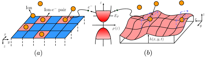
Figure 1: Two examples showing the evolution of electrochemical interfaces driven by chemical reactions. (a) The first example corresponds to ion intercalation, where ions and electrons are inserted in concerted way at a free spot on the solid interface (blue cells). Because of the attractive interactions of the ion-$e^{-}$ pairs with each other, the interface species might undergo a phase separation Bai, Cogswell, and Bazant (2011); Lim et al. (2016) (b) The second example is related to film growth, where again, ions are ‘adsorbed’ at a reduced spot on the existing substrate of height $h$. Curvature effects Mullins (1957) lead to inhomogeneous film growth, which finally leads to island formation during electrodeposition Horstmann et al. (2013).

II Theory

In the present work, we analyze the evolution of interfacial morphology controlled by electrochemical reactions, described by the phenomenological Butler-Volmer equation Newman and Thomas-Alyea (2004), electron-transfer (ET) theories Kuznetsov and Ulstrup (1999), or coupled ion-electron transfer (CIET) theory Fraggedakis et al. (2020). Herein, we briefly describe the main idea behind the general reaction rate theory, explain the differences between different Faradaic reaction rate models, and demonstrate under which conditions they apply based on the application of interest. Additionally, we want to control the morphology of interfaces where Faradaic reactions take place. To do so, we follow the general analysis from Ref. Bazant (2017) and make use of non-equilibrium thermodynamic stability criteria for constructing phase diagrams in terms of the operational conditions for ion intercalation Bai, Cogswell, and Bazant (2011) and thin film growth Horstmann et al. (2013).

II.1 Reaction Kinetics

For the simple reduction reaction of cations $O^{+}$

$$O^{+}+e^{-}\leftrightarrows R$$

one expresses the net reaction rate $R_{t}$ as the difference between the forward $R_{\rightarrow}$ and the backward $R_{\leftarrow}$ elementary rates. These are described by the general theory of non-equilibrium thermodynamics, Christov (2012); Keizer (2012); Bazant (2013), which is based on Transition State (TS) theory Truhlar, Hase, and Hynes (1983). The energy of the participating species $i$ as well as the TS energy are described by their chemical potential $\mu_{i}$.

Generally, when electrochemical reactions (Faradaic or not) are considered it is common practice to apply Butler-Volmer kinetics Bard and Faulkner (2001); Newman and Thomas-Alyea (2004); Butler (1924); Erdey-Grúz and Volmer (1930) to describe the current $I$ as a function of the thermodynamic driving force, e.g. overpotential $\eta$. As has been shown in Bazant (2013); Keizer (2012), the model is rigorously derived by assuming the TS barrier $\mu_{\ddagger}$ to be the weighted average of the reactant and product standard electrochemical potentials, where the weights are directly related to the charge transfer coefficient $\alpha$. However, the BV model is purely phenomenological and thus its parameters are not directly related to material properties Kuznetsov and Ulstrup (1999).

Fig. 2(a) shows the reaction energy landscape for BV kinetics in terms of an arbitrary reaction coordinate, e.g. distance of reacting species from electrode surface. In all cases, $x_{O}$ and $x_{R}$ denote the equilibrium coordinates of the reactant and product states, respectively, while $x_{\ddagger}$ corresponds to the TS point. At equilibrium, thermal fluctuations need to provide sufficient energy to the reactants for transforming them into products. By applying a small driving force $\eta_{1}$ in the system (red curve), both the energy of the reactants and that of the TS point increase, but overall the absolute difference between those two decreases. Therefore, the external bias favors the reduction reaction. If larger overpotential is applied, i.e. $\eta_{2}$, the energy state of the reactants overcomes the TS barrier, leading to an effectively barrier-less reaction (orange curve). That said, in the BV picture there is a critical value of the applied driving force above which the resulting net reaction rate $R_{t}$ (or current $I=eR_{t}$) increases indefinitely. However, for several bulk or Faradaic reactions this trend does not apply. The current is either known to reach a limiting value with increasing $\eta$ or to show a non-monotonic behavior, where at first the current increases and after a critical $\eta$ it decreases. The region after which $I$ decreases with increasing $\eta$ is called the Marcus inverted region and is associated with the electron transfer event Marcus (1965, 1993); Kuznetsov and Ulstrup (1999); Schmickler and Santos (2010).

Electron transfer reactions are described by the theory introduced by Marcus, and further developed by Hush, Dogonadze, Kuznetsov, Levich and others Marcus (1956, 1965); Levich (1966); Levich and Dogonadze (1963); Kuznetsov and Ulstrup (1999); Hush (1961); Schmickler (1986); Schmickler and Santos (2010). The main mechanism of ET involves the interactions of the electron $e^{-}$ participating in the reaction with the environment of the molecule/atom (solvent molecules or crystal atoms) that is reduced/oxidized. Fig. 2(b) demonstrates the excess energy landscape for an ET reaction as a function of the reaction coordinate. Under this picture, the electrons are considered to be ‘localized’ either in the reactant or product state (two-state system), while the environment undergoes thermal fluctuations. The parabolas shown represent the degree of polarization of the solvent environment. A mechanistic picture of an ET reaction is the following. Consider the equilibrium case (blue curve) for $x=x_{O}$, where the reactants (dark blue particle) have a solvation shell of a particular structure (orange square). Thermal fluctuations may provide enough energy to the environment helping the reactants to reach $x=x_{\ddagger}$. There, the solvation shell has a structure which combines that of the reactants and the products one (orange square and bluish circle). Once this happens, the electron reduces the reactants species and the ET event is successful. The same mechanism is true for the reverse reaction (oxidization). The ET concept is very similar to polaron hopping, which was introduced by Landau Landau (1933), and further developed by Pekar, Fröhlich, Holstein Pekar and Deigen (1948); Fröhlich, Pelzer, and Zienau (1950); Holstein (1959a, b); Toyozawa (1954) at around the same time as Marcus published his first paper on bulk ET.

A fundamental concept of ET theories is the reorganization energy $\lambda$ Schmickler and Santos (2010); Kuznetsov and Ulstrup (1999); Bazant (2013). Its physical interpretation is understood via the following example. Consider the products excess energy landscape at equilibrium $x=x_{R}$ where the products (green circle) have a specific solvation shell structure (bluish green). The reorganization energy is defined as the energy required to transform the solvation shell of the products to that of the reactants without an electron transfer to take place (green circle with orange square). The same definition is given from the reactants perspective, where a different value for $\lambda$ may be defined. In the present work, we are going to limit ourselves to the same reorganization energy for both reactants and products.

As discussed earlier, the magnitude of the applied bias $\eta$ affects the behavior of the resulting current $I$. For low overpotential (red curve), the energy of the reactants increases leading to a decrease in the TS barrier, fig. 2(b). As in BV model, there is a critical $\eta$ (orange curve) where the TS barrier becomes zero and the reaction becomes barrier-less. However, further increase in the applied bias (green curve) does not lead to zero activation energy, rather it starts increasing it again ($\Delta\mu^{ex}=\mu^{ex}_{\ddagger}-\mu^{ex}_{O}>0$). This phenomenon leads to the celebrated Marcus inverted region where $I$ decreases with increasing $\eta$.

In bulk ET theory, the electron participating in the reaction has a single energy level $\varepsilon$. In most electrochemical systems, though, a reaction occurs nearby an electrode which supplies electrons that occupies a spectrum of energy levels (Faradaic reaction). Therefore, the density of states (DOS) of the electron donor plays a crucial role in defining the dynamics of electron transfer, as well as the final structure of the interface on which the Faradaic reaction takes place. To determine the overall reaction rate, one has to integrate over all the available energy electron levels, resulting in Kuznetsov and Ulstrup (1999); Schmickler and Santos (2010); Zeng et al. (2014)

$$R_{t}=\int\rho(\varepsilon)\left(R_{\rightarrow}(\varepsilon)-R_{\leftarrow}(\varepsilon)\right)d\varepsilon$$ (1)

Herein, we are interested on how different DOS models affect the stability of electrochemical interfaces. In particular, we focus on the differences between a localized electron state and that of a delocalized one. In the former case, the DOS is $\rho(\varepsilon)=\delta(\varepsilon-\varepsilon_{i})$, which leads to the so-called Marcus model, while in the second one, the DOS of a metallic donor is considered. To a good approximation, the metallic DOS is described by $\rho(\varepsilon)=1$ recovering the Marcus-Hush-Chidsey (MHC) model Chidsey (1991). In this case, when the driving force (overpotential) becomes larger than the reorganization energy $\lambda$, the celebrated ‘inverted-region’ is lost because electrons from multiple energy states contribute to the total reaction rate, leading to what is known as reaction-limited current Kuznetsov and Ulstrup (1999); Fraggedakis et al. (2020). Of course, different electron donor DOS can be used, e.g. for semi-conductors, semi-metals, etc. Schmickler et al. (2017), though the final conclusion on the stability of electrochemical interfaces does not change.

Fig. 2(d) illustrates the Tafel plot for the three models considered, namely the BV, Marcus, and MHC constitutive relations. For BV, it is well-known that $I$ increases indefinitely with increasing $\eta$. For the other two cases, though, when $\eta\geq\lambda$ the current either reaches its maximum value and then decreases (Marcus model) or it attains a limiting value $I\left(\eta\rightarrow\infty\right)\simeq I_{max}$ (MHC model).

Up to this point, we described extensively the physics of different Faradaic reaction models which contain only one electron transfer as the rate limiting step. Although we have not discussed about the formulation of coupled ion-electron transfer (CIET) kinetics, the main idea is similar to the classical ET picture. CIET is based on the concerted transfer of both an ion and an electron, where the ion transfer is being described by classical transition state theory while that of the electron is based on Marcus kinetics. More details about the mathematical derivation of the model is found in Fraggedakis et al. (2020), where the theory is shown to describe quantitatively the insertion of Li ions in FePO₄ (FP) Lim et al. (2016); Li et al. (2018).

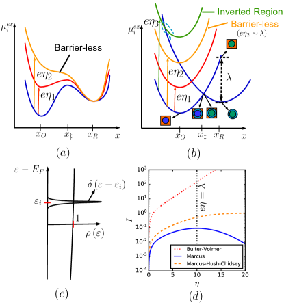
Figure 2: Excess energy landscape of reactant ($O$)- product ($R$) species as a function of the reaction coordinate for (a) Butler-Volmer kinetics (b) electron transfer. The reaction coordinate points $x=x_{O}$ and $x=x_{R}$ correspond to the equilibrium points of the reactants (oxidized) and products (reduced) species, respectively. In both models the transition state barrier is located at $x=x_{\ddagger}$. (c) Examples of the electron donor density of states considered in this work. (d) Current $I$ vs. applied overpotential $\eta$ for Butler-Volmer kinetics (red dotted curve), Marcus kinetics (blue curve), and Marcus-Hush-Chidsey model (orange dashed curve).

II.2 Electrochemical Stability

n Very recently, it was shown that this is not always the case Bazant (2017), and the thermodynamic stability of a solution is controlled by using non-equilibrium driving forces. When the reaction rate depends on the concentration of the participating species, in addition to their chemical potentials, solo-autocatalytic/inhibitory effects participate on determining the homogeneity of the solution. Therefore, when a chemical reaction is auto-inhibited, that means with increasing products concentration the reaction rate decreases, there is a critical value in the driving force after which the system becomes thermodynamically stable. A characteristic example of such behavior is the lithiation of Li_xFePO₄ Bai, Cogswell, and Bazant (2011); Cogswell and Bazant (2012); Li et al. (2014); Lim et al. (2016); Nadkarni et al. (2018); Li et al. (2018); Nadkarni et al. (2019); Gonzalez-Rosillo et al. (2020) in which the net reaction rate is a decreasing function of the concentration Fraggedakis et al. (2020); Lim et al. (2016).

II.2.1 Basic Formalism of linear stability

Herein, our main focus is to analyze the simple reaction described in Sec.II.1. Also, we consider the reactants to be drained from a reservoir, while the system contains only the products. The reaction is driven either under constant rate $R_{t}$ or under constant reservoir chemical potential $\mu_{res}$. In electrochemical systems these conditions are translated into constant current $I$ and constant electrode voltage $V$, respectively.

We are interested in understanding the linear stability of the order parameter $c$, which can represent either the local species concentration or the height of a domain. The general evolution equation for $c$ under reaction-limited growth is Bazant (2013)

$$\frac{\partial c}{\partial t}=R$$ (2)

where $R$ is the reaction rate. In general, $R$ is expressed as a function of $c$, its chemical potential $\mu$, and in open systems the reservoir chemical potential $\mu_{res}$.

For phase separating systems, the following form of the free energy $G$ is assumed

$$G[c,\nabla c]=\int_{V}\left(g_{h}\left(c\right)+\frac{1}{2}\kappa\lvert\nabla c\rvert^{2}\right)dV$$ (3)

where $g_{h}(c)$ is the homogeneous energy and $\kappa$ is the penalty gradient term, which is related to the energy required to form an interface in the bulk solution Cahn and Hilliard (1958); Rowlinson (1979). Hence, the chemical potential $\mu$ is defined as the variational derivative of $G$

$$\mu=\frac{\delta G}{\delta c}=\frac{\partial g_{h}}{\partial c}-\kappa\nabla^{2}c$$ (4)

In this work, we examine the stability of an initially homogeneous solution with mean order parameter $\bar{c}$. Under infinitesimal perturbations, the concentration profile is of the form

$$c({\mathbf{x}},{t})=\bar{c}+\varepsilon e^{\sigma t-i\mathbf{k}\cdot\mathbf{x}}$$

where $\sigma$ corresponds to the growth rate of the perturbation and $\mathbf{k}$ to its corresponding wave vector. Substituting $c(\mathbf{x},t)$ in eq. 2 and keeping the first order terms in $\epsilon$ only, the following equation for the growth rate results

$${\sigma}=\frac{\partial{R}}{\partial c}+\frac{\partial{R}}{\partial{\mu}}\frac{\delta{\mu}}{\delta c}$$ (5)

and substituting $\frac{\delta{\mu}}{\delta c}=\frac{\partial{\mu}_{h}}{\partial c}+{\kappa}k^{2}$ one arrives at Bazant (2017)

$${\sigma}=\frac{\partial{R}}{\partial c}+\left(\frac{\partial{\mu}_{h}}{\partial c}+{\kappa}{k}^{2}\right)\frac{\partial{R}}{\partial{\mu}}$$ (6)

Following the analysis in Bazant (2017) for the wavelength $k$ that maximized the growth rate $\sigma$, the stability window is determined by solving the following equation for the critical operation conditions

$$\widetilde{\sigma}\left(c,\widetilde{I}_{c},\widetilde{V}_{c}\right)=\frac{\partial\widetilde{I}}{\partial c}+\frac{\partial\widetilde{I}}{\partial\widetilde{\mu}}\frac{\partial\widetilde{\mu}}{\partial c}=\widetilde{\tau}^{-1}$$ (7)

where $\left(\widetilde{I}_{c},\widetilde{V}_{c}\right)$ correspond to the critical value of the external bias, and $\tau$ is the characteristic time required to complete the process, e.g. the time required to fully intercalate the system Bai, Cogswell, and Bazant (2011) or the time to deposit an atomic layer Horstmann et al. (2013). All quantities with $\,\,\widetilde{}$   are dimensionless. Also, $\widetilde{\sigma}$ is known as the dispersion relation Bazant (2017). The detailed derivation of eq. 7 when solid diffusion is considered is given in the Appendix.

According to classical linear stability theory, when $\widetilde{\sigma}>0$ the process is unstable and it diverges from its base state, while for $\widetilde{\sigma}<0$ all the applied perturbations decay in time and stability is preserved. In the context of ion intercalation, instability means the separation of the ionic solution in two regions, one ‘rich’ and one ‘poor’ in ions. For film growth, though, $\widetilde{\sigma}>0$ translates either into the film growth with increased surface roughness Kardar, Parisi, and Zhang (1986) or the formation of localized islands Horstmann et al. (2013) in the nanoscale Khoo, Zhao, and Bazant (2019). Eq. 7 shows that different reaction rate mechanisms will result in different stability behavior. Therefore, by understanding how the microscopic physics and the material properties alter the phase diagram, we will be able to operate the process of interest under optimal conditions. Additionally, the theory can be used to provide engineering guidelines on the materials selection and device design to achieve the desired results.

II.3 Thermodynamics and Reaction Models for Ion intercalation and Film Growth

II.3.1 Ion Intercalation

In the case of ion intercalation Bai, Cogswell, and Bazant (2011), it is common practice to use the regular solution model to describe phase-separating materials. The form of the homogeneous free energy $g_{h}(c)$ reads

$$g_{h}(c)=\Omega c\left(1-c\right)+k_{B}T\left(c\ln c+(1-c)\ln(1-c)\right)$$ (A.11)

where $\Omega$ is the species attraction energy, $c$ is the concentration of the inserted species and $1-c$ is the concentration of the vacancies. This model corresponds to a lattice gas. The only free parameter in eq. A.11 is $\Omega/k_{B}T$ which, in this study, we set $\Omega/k_{B}T=4.0$ corresponding to LiFePO₄ at room temperature Bai, Cogswell, and Bazant (2011).

Here, three different reaction models are considered. These are the coupled ion-electron transfer for a metallic and a localized density of states and the Butler-Volmer model. The general reaction rate for the case of coupled ion-electron transfer is

$$R=\int_{-\infty}^{\infty}\rho\left(\varepsilon\right)k_{0}\left(n\left(\varepsilon\right)(1-c)e^{-\frac{\left(\lambda+\eta_{f}-\varepsilon\right)^{2}}{4\lambda}}-(1-n\left(\varepsilon\right))ce^{-\frac{\left(\lambda-\eta_{f}-\varepsilon\right)^{2}}{4\lambda}}\right)d\varepsilon$$ (8)

where $n\left(\varepsilon\right)$ is the Fermi-Dirac distribution and $\eta_{f}=\mu-\mu_{res}-\ln c/(1-c)$. Unless otherwise specified, we set $\lambda/k_{B}T=8.3$ Bai and Bazant (2014).

II.3.2 Film Growth

For the film growth, we adopt a thermodynamics model that is commonly used in epitaxial growth, and has been shown to describe qualitatively the formation of Li₂O₂ in Li-air batteries Horstmann et al. (2013). The model for the homogeneous Gibbs free energy is

$$g_{h}(h)=\frac{2e}{d_{\bot}\pi}\left[-E_{0}\pi h+E_{1}\sin^{2}\left(\pi h\right)-E_{2}e^{-\beta h^{2}/2}\right]$$ (9)

where $h$ is the height of the film. The physical meaning of the parameters $E_{0}$, $E_{1}$, $E_{2}$ and $\beta$, as well as their values, are described in Horstmann et al. (2013). For film growth, the ET-based reaction model expression is

$$R=\int_{-\infty}^{\infty}\rho\left(\varepsilon\right)k_{0}\left(n\left(\varepsilon\right)e^{-\frac{\left(\lambda+\eta_{f}-\varepsilon\right)^{2}}{4\lambda}}-(1-n\left(\varepsilon\right))e^{-\frac{\left(\lambda-\eta_{f}-\varepsilon\right)^{2}}{4\lambda}}\right)d\varepsilon$$ (10)

where $n\left(\varepsilon\right)$ is the Fermi-Dirac distribution and $\eta_{f}=\mu(h)-\mu_{res}$.

III Results

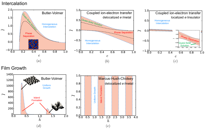
Figure 3: Phase stability diagrams for ion intercalation (a)-(c), and film growth (d)-(e), under applied constant current $\left(\widetilde{I}\right)$ conditions for different electrochemical reaction models. The light red region corresponds to the linearly unstable region, where phase separation is predicted to occur. The marginal stability curve is denoted with the light-blue dashed line. For ion intercalation, the black dashed line is used to describe the boundary of the quasi-solid solution, the region in which the applied perturbation does not have enough time to evolve until the process ends. The results for Butler-Volmer kinetics are shown in (a) and (d), while the results for the ET models are illustrated in (b),(c) and (e). For demonstration purpose snapshots of the system state at specific $c/\widetilde{h}$ are shown for the Butler-Volmer model. ET-based models produce qualitatively similar results.

Our main scope is to show the differences on the predicted stability diagrams for different electrochemical reaction models, e.g. the phenomenological BV kinetics and the electron transfer theories. The comparison is performed in terms of ion intercalation and thin film growth.

Fig. 3 illustrates the non-equilibrium phase diagrams in terms of the dimensionless imposed current, and the state of the system (ion concentration $c$ in ion intercalation, film height $\widetilde{h}$ in film growth). At first sight, the differences in the predictions between BV and the ET models are apparent. Not only they differ quantitatively, but the regions which are linearly unstable (light red color) have qualitatively different bounds.

This behavior is explained in physical grounds by examining the predictions for each process separately. Irrespective of the reaction mechanism ion intercalation is known to be a solo-autoinhibitory process, $\partial\widetilde{I}/\partial c<0$  Bazant (2017); Lim et al. (2016); Bai, Cogswell, and Bazant (2011). Therefore, a different mechanism is required to affect the second term in eq. 7 which couples the thermodynamic stability via $\partial_{c}\widetilde{\mu}$ with the changes of $\widetilde{I}$ as a function of $\widetilde{\mu}$. For BV kinetics, it is easily shown that $\partial\widetilde{I}/\partial\widetilde{\mu}=-\partial\widetilde{I}_{\leftarrow}/\partial\widetilde{\mu}\sim-e^{\widetilde{\mu}}$. On the other hand, for Marcus/MHC models the sign of $\partial\widetilde{I}/\partial\widetilde{\mu}$ is not definite, and it changes with different values of the thermodynamics driving force $\widetilde{\eta}=\widetilde{V}+\widetilde{\mu}$. Therefore, the exact reaction mechanism, and thus its mathematical form, is crucial to understanding the thermodynamic stability of a far-from equilibrium system. Having this in mind, it is not surprising why different phase diagrams for BV, Marcus and MHC kinetics are produced. In particular, for BV, phase separation is suppressed solely due to the inhibitory nature of the reaction. On the contrary, both CIET models involve not only the contribution of ions at the TS but also the effects of the thermodynamic state of the system on the electron transfer mechanism via $\widetilde{\mu}$ Fraggedakis et al. (2020).

Returning to figs. 3(a)-(c), it is apparent that all models predict suppression of phase separation for $\widetilde{I}>\widetilde{I}_{c}(c)>0$. Here $\widetilde{I}_{c}$ corresponds to the critical current (light dashed line) obtained after solving $\widetilde{\sigma}\left(c,\widetilde{I}_{c},\widetilde{V}_{c}\right)=0$. The stability boundary differs between BV and CIET models as a result of the convoluted effects of ion and electron transfer phenomena. More specifically, those effects are shown in fig. 2(d) where for the same overpotential BV predicts the largest value of $\widetilde{I}=\widetilde{I}_{BV}$, Marcus model has the lowest value on $\widetilde{I}=\widetilde{I}_{M}$, while MHC predictions ($\widetilde{I}=\widetilde{I}_{MHC}$) are in between the two other models $\widetilde{I}_{BV}>\widetilde{I}_{MHC}>\widetilde{I}_{M}$.

The main differences between the models predictions occur for de-intercalation. Systems following BV kinetics are predicted to always be unstable when $\widetilde{I}<0$, as the process becomes solo-autocatalytic in the reverse direction Bazant (2017). This is not the case for ET models where an extended thermodynamically stable region is present. The in-situ experiments performed by Lim et al. Lim et al. (2016) on the delithiation of Li_xFePO₄ showed that under moderate to large charging rates, LFP particles did not undergo phase separation, an observation that cannot be explained using BV kinetics Bazant (2017); Li et al. (2018). Combining this result with the predicted stability diagram for the CIET-MHC model which shows a thermodynamically stable region upon charging, fig. 3(b), we are able to say that LFP is a coupled ion-electron transfer limited material Fraggedakis et al. (2020). Now, comparing the results between the two ET models, we conclude that under smaller values of the applied current, electrons with localized energy levels tend to stabilize even further the system, fig. 3(c).

For film growth the predicted non-equilibrium phase diagrams are very different to each other, fig. 3(d)-(e). For conciseness we show only the results for one ET model (MHC) as their predictions are qualitatively similar. Following Horstmann et al. Horstmann et al. (2013), $\widetilde{I}_{c}(\widetilde{h})$ is predicted from $\widetilde{\sigma}\left(\widetilde{h},\widetilde{I}_{c},\widetilde{V}_{c}\right)=\widetilde{I}$. In this case, the transition state does not include ionic effects such as excluded volume Bai, Cogswell, and Bazant (2011). That translates into $\partial\widetilde{I}/\partial\widetilde{h}=0$ which makes the stability to be solely determined by balancing the second term of eq. 7 with the characteristic time $\widetilde{\tau}^{-1}=\widetilde{I}$. Here $\widetilde{\tau}$ is the time required to fully deposit an atomic layer of height $\Delta\widetilde{h}=\widetilde{h}_{i+1}-\widetilde{h}_{i}=1$.

Clearly, under constant $\widetilde{I}$ the non-equilibrium stability diagram produced using ET models coincide with the equilibrium thermodynamics one, fig. 3(e). There are two reasons for this behavior. At first, the changes in the film chemical potential with $\widetilde{h}$ are abrupt, leading to large values of $\partial\widetilde{\mu}/\partial\widetilde{h}$. Additionally, the process attains current values which are limited by electron transfer, fig. 2(d), resulting in $\left\lvert{\partial\widetilde{\mu}}/{\partial\widetilde{c}}\right\rvert\gg\widetilde{I}\left({\partial\widetilde{I}}/{\partial\widetilde{\mu}}\right)^{-1}$ for all $\widetilde{h}$ and $\widetilde{I}$.

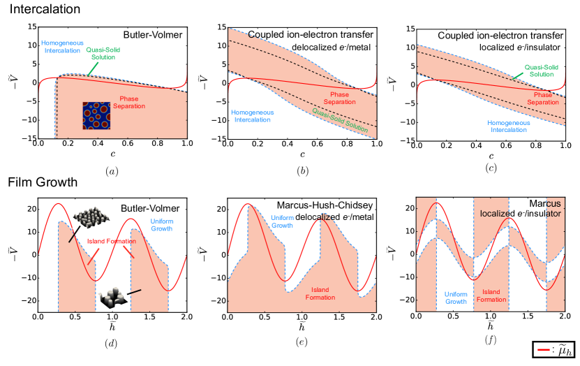
Figure 4: Phase stability diagrams for ion intercalation (a)-(c), and film growth (d)-(f), under applied constant voltage $\left(\widetilde{V}\right)$ conditions for different electrochemical reaction models. The light red region corresponds to the linearly unstable region, where phase separation is predicted to occur. The red line corresponds to the system homogeneous chemical potential. The marginal stability curve is denoted with the light-blue dashed line. For ion intercalation, the black dashed line is used to describe the boundary of the quasi-solid solution, the region in which the applied perturbation does not have enough time to evolve until the process ends. The results for Butler-Volmer kinetics are shown in (a) and (d), while the results for the ET models are illustrated in (b),(c),(e) and (f). For demonstration purpose snapshots of the system state at specific $c/\widetilde{h}$ are shown for the Butler-Volmer model. ET-based models produce qualitatively similar results.

For BV kinetics, the same thermodynamic stability argument is true, but the model predicts indefinite large values for $\widetilde{I}$ which is not realistic. This is the main reason Horstmann et al. Horstmann et al. (2013) were able to predict suppression of inhomogeneous Li-O₂ film growth, fig. 3(d). However, the predictions of fig. 3(d) do not imply much regarding the reaction mechanism of Li-O₂ formation. The linear stability results correspond to the initial stages of interfacial instability. As in the case of LFP, large enough current lead to a quasi-homogeneous film profile because there is not enough time for the instability to grow Bai, Cogswell, and Bazant (2011). In fact, as shown in fig. 1(c) of Horstmann et al. (2013) the structure of the ‘homogeneous’ film show the existence of some Li₂-O₂ microstructure on the CNT surfaces Gallant et al. (2012); Mitchell et al. (2013). Thus, it is possible Li₂-O₂ growth to be electron transfer limited, a fact that is supported by the experimentally observed and ab-initio predicted curved Tafel plots Viswanathan et al. (2013).

Not only constant $\widetilde{I}$, but also constant voltage $\widetilde{V}$ stabilize an unstable solution. Fig. 4 shows the predicted phase diagrams under non-equilibrium conditions for both ion intercalation, figs. 4(a)-(c), and film growth, figs. 4(d)-(f). Additionally, the chemical potential $\widetilde{\mu}$ of the products is included (red thick line) to highlight the departure from equilibrium via $\widetilde{\eta}\left(c\right)$.

For ion insertion ($-\widetilde{V}>\widetilde{\mu}$) all models predict suppression of any instability for a wide range of $\left(-\widetilde{V},c\right)$, figs. 4(a)-(c). In general, under applied voltage the overpotential varies with time $\widetilde{\eta}(c)\simeq\widetilde{V}+\widetilde{\mu}(c)$ as a result of $c\left(\widetilde{t}\right)=\int_{0}^{\widetilde{t}}\widetilde{I}(\widetilde{\eta})d\widetilde{t}^{\prime}$. When the solution enters the spinodal region, $\widetilde{\mu}\left(c\right)$ becomes a decreasing function leading to continuously increasing $\widetilde{\eta}$, and thus to increasing $\widetilde{I}$. This behavior gives an advantage to phase separating materials for Li-ion battery applications, as under constant $\widetilde{V}$ conditions not only we stabilize their thermodynamic state but we also achieve higher (dis)charging rates.

From figs. 4(a)-(c), BV kinetics predict more stable ion insertion compared to ET models. Let us consider the case with $-\widetilde{V}=5$. For BV the solution starts and remains inside the thermodynamically stable region for all the values of $c$ along the process. This is not true for MHC and Marcus models, though, where the material is predicted to be unstable from $c=0$ to approximately $c\simeq 0.6$, and there is high probability for phase separation. The reason why this happens is understood in terms of the resulting current, which as discussed earlier, changes with increasing $c$. The evaluated $\widetilde{I}$ using BV under $\widetilde{V}=-5$ is always larger than the marginal stability boundary $\widetilde{I}_{c}(c)$ shown in fig. 3(a). On the other hand, when the reaction mechanism is associated with electron transfer $\widetilde{I}$ falls into the unstable region, figs. 3(b)-(c), and therefore the solution tends to phase separate.

The conclusions for de-intercalation ($-\widetilde{V}<\widetilde{\mu}$) are very similar to the case of constant current. BV is found to be unstable for almost all sets of $\left(-\widetilde{V},c\right)$, while ET models predict suppression of phase separation. Again, when the donated electron has a single energy the differential negative resistance, $\partial\widetilde{I}/\partial\widetilde{\mu}<0$, tends to stabilize the system more effectively than in the case of a continuous energy spectrum.

When film growth is driven under constant $\widetilde{V}$, one is able to observe very interesting behavior on the resulting phase diagrams. In particular, while under constant $\widetilde{I}$ the ET stability was determined solely by thermodynamics, fig. 3(e), here it is found that homogeneous film growth is stable for a wide range of applied potentials $\widetilde{V}$. When only localized electrons participate in the reaction the negative differential resistance starts playing a more active role in the stabilization mechanism. In fact, as shown from fig. 4(f), there is an interchange between stable and unstable regions. More specifically, with increasing driving force the current enters the Marcus inverted region altering the sign of $\partial\widetilde{I}/\partial\widetilde{\mu}$ in eq. 7, and thus turning a thermodynamically stable growth to an unstable one Bazant (2017).

The results shown in figs. 3 & 4 correspond to a specific set of material parameters. Briefly, for the intercalation case large values of the reorganization energy $\lambda$ tend to induce stability under constant current conditions, as the reaction activation barrier $E_{act}\sim\lambda/4k_{B}T$ increases Marcus (1993); Bazant (2013); Fraggedakis et al. (2020). On the contrary, for constant $V$ higher values of $\lambda$ destabilize the thermodynamics solution.

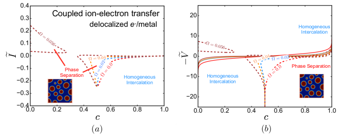
Figure 5: Effect of the ion attraction energy on the non-equilibrium phase diagrams for coupled ion-electron transfer. In (a) we control applied current $\tilde{I}$, while in (b) we change the applied voltage $\tilde{V}$.

The effects of thermodynamics factors, such as the interaction parameter $\Omega$, affect the non-equilibrium stability of the process, fig. 5. In particular, with increasing attractive interactions between ions (large $\Omega$ values), the area of the unstable region increases changing the non-equilibrium phase diagram. Of interest is the case of $\Omega=0$ (no attractions) where the material is essentially in the solid-solution regime (single phase). When ions are extracted from the system ($\widetilde{I}<0$) CIET-ET models tend to destabilize the solution, inducing a non-thermodynamically favored phase separation Bazant (2017). This is caused by the solo-autocatalytic nature of de-intercalation and has a significant impact on the stability of several materials like those used in Li-ion batteries. A representative example is NCM which is known to be a solid solution material Yabuuchi and Ohzuku (2003); Jouanneau et al. (2003). However, as it is shown in Gent et al. (2016); Grenier et al. (2017); Zhou et al. (2016) for a population of cathode particles, during de-lithiation the solid solution can be destabilized leading to Li-poor and Li-rich phases. This phenomenon has been demonstrated theoretically very recently, by using population dynamics to describe the kinetics on the porous electrode scale Zhao and Bazant (2019b).

IV Discussion

The results of the considered ET models stress the importance of the electron donor density of states on the morphology of electrochemical interfaces. In general, it is shown that the more localized are the electrons that participate in the electrochemical reaction, the greater the thermodynamic stability of the process. That means, when the electrons that participate in the electrochemical reaction are initially localized, or reside in low-dimensional materials (e.g. quantum dots), then phase separation in ion intercalation or island formation in epitaxial growth is less likely to be observed. Physically, the reason for stabilization of the interface morphology is that the more localized, poorly available electrons suppress autocatalysis and can even lead to auto-inhibitory kinetics, e.g. in the Marcus inverted region of negative differential reaction resistance Bazant (2017).

Our findings demonstrate new ways on tuning interfaces to have the desired topology. This is achieved by either controlling the driving force (current or voltage) of the reaction in a time-varying way, or by modifying the density of states of the electron donor, e.g. by doping. The desired topology for each application varies. For example, in (electro)catalysis it is desired to grow interfaces that have large surface area, fig. 6(a).

In energy storage via Li-ion intercalation, we want to minimize the occurrence of phase separation, as the formation of different phases on interfaces cause the development of large elastic stresses which usually lead to fracture or delamination of the active material, fig. 6(b). Large elastic stresses between the active material and solid electrolyte may cause loss of contact, and therefore induce capacity fading in the long-term operation of the battery. This is the case in all-solid-state batteries, where inhomogeneous intercalation of Li ions leads to expansion of the host material, and consequently delamination Koerver et al. (2017). In commercial Li-ion batteries, the use of phase-separating materials (e.g. LiFePO₄, LiCoO₂, Li_xC₆) leads to the formation of interphases during operation. As a result, elastic stresses due to lattice mismatch develop which cause electrode particles to crack.

Another example is energy harvesting via light absorption, where the structure of the interface exposed to light should minimize the reflection to absorption ratio, fig. 6(c). The efficiency of light-absorbing devices depends on the manufacturing conditions as the manufactured interfaces need not to be ‘rough’. A characteristic example is the deposition of Cu on Zn for high-efficiency solar–thermal energy conversion Mandal et al. (2017). The theory presented herein can be used as a guideline for the optimal selection of the manufacturing conditions, in order to produce interfaces with the desired structure.

The same is true in photocatalytic applications, where while we desire large active surface area, the emitted light can be reflected, and thus lead to low conversions. There are cases where parasitic reactions affect the topology of the surface by forming a passivation film, fig. 6(d), which effectively decreases the active surface area and increases light reflection, respectively. While avoiding the formation of the film is difficult, we can choose the operating conditions where island formation is favorable compared to homogeneous film formation, e.g. by holding the surface voltage to levels that promote island formation.

Our model is formulated in a general way that implicitly captures system-environment interactions, e.g. double layer structure, ion (de)solvation energies, active surface area, etc., in terms of a lumped reaction constant. The present theory provides the basis to understand from first-principles the stability of interfaces undergoing electrochemical reactions, a factor which affects the performance of several applications related to energy harvesting and storage, catalysis, and electrocatalysis.

Finally, the current status of the theory neglects elastic strain effects, which is particularly important in epitaxial growth. To include these phenomena, a more complete model is required that takes into account the formation of dislocations, as well as the spatial dependence of the developed strain upon film formation. Additionally, the formation of voids, as well as the diffusion of vacancies underneath the studied interface are expected to affect our stability results. In a future work, we will develop a general model of multilayer epitaxial growth using electrochemical reactions that takes into account the missing aspects of the present theory, and show how to exploit them to tune the morphology of interfaces.

V Conclusions

A comprehensive stability theory is presented to predict the effects of electron-transfer reaction kinetics in controlling the morphology of electrochemical interfaces The theory was applied successfully on two technologically relevant processes, those of ion intercalation and surface growth driven by electrochemical reactions.

Using the recently developed non-equilibrium thermodynamics framework for open-driven systems Bazant (2017), we studied the performance of different electron transfer models on stability of a thermodynamically unstable system. In particular, we focused on the ubiquitous, but phenomenological, Butler-Volmer kinetics and on electron transfer models, which include details of the quantum/microscopic nature of the materials participating in the process (e.g. density of states of electron donor, reorganization energy of the electron environment, etc.).

When ion intercalation is described by coupled ion-electron transfer kinetics, the process is found to be homogeneous for a larger set of the applied driving force (current $I$ or voltage $V$) with the fractional concentration $c$, compared to the BV analog. On the contrary, ET-limited surface growth is predicted to always be unstable under fixed current, leading to surfaces with increased roughness and ultimately to island formation. This is not the case when $V$ is being controlled, where ET models show a more complex behavior.

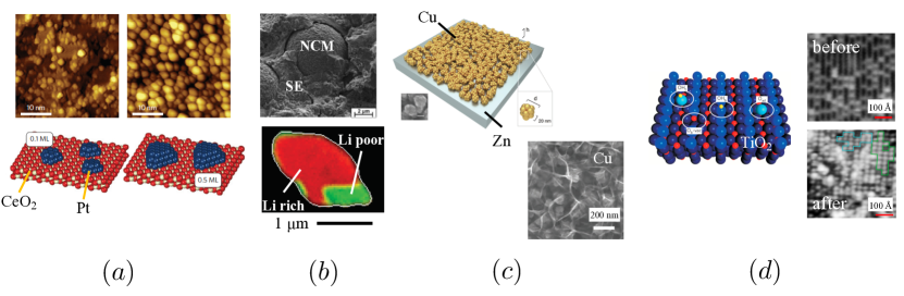
Figure 6: (a) Growth of Pt nanoparticles on CeO₂ substrate for applications related to catalysis. The number of electrons that are transfered during the deposition of Pt particles on CeO₂ control the structure of the catalytic interface. Figures are adapted from Lykhach et al. (2016). (b) Examples related to Li-ion intercalation in NCM and LFP. The development of stresses at interfaces between active material and solid electrolyte may cause loss of contact, and therefore induce capacity fading in the long-term operation of the battery. Figures are adapted from Koerver et al. (2017); Lim et al. (2016). (c) The efficiency of light-absorbing interfaces for energy storage depends on the manufacturing conditions. More specifically, it is crucial to maximize the absorption to reflection ratio. To achieve high absorption to reflection ratio, the interfaces need not to be ‘rough’. Figures are adapted from Mandal et al. (2017). (d) Interfaces used in photocatalysis are desired to have high absorption-to-reflection ratio and large active surface area. There are cases where parasitic reactions affect the topology of the surface by forming a passivation film. We can operate the process under conditions where island formation is favorable compared to homogeneous film formation. Figures are adapted from Hussain et al. (2017).

Data Availability Statement

The data that supports the findings of this study are available within the article.

Appendix

Derivation of Stability Criterion

The system is connected to a reservoir of constant temperature $T_{rev}$, pressure $P_{res}$ and number of particles $N_{rev}$. The adsorption process is described by the following conservation law

$$\frac{\partial c}{\partial t}=-\nabla\cdot\mathbf{j}+R$$ (A.1)

where $c=N/N_{max}$ corresponds to the fractional concentration in the system, $\mathbf{j}$ is the mass flux vector and $R$ denotes the ‘volumetric’ reaction rate. Both the flux Keizer (2012) and reaction rates Bazant (2013) are formulated based on macroscopic non-equilibrium thermodynamics as follows

$$\mathbf{j}=-M(c)c\nabla\mu$$ (A.2)

$$R=k_{o}e^{-\mu^{ex}_{\ddagger}/(k_{B}T)}\left(e^{\mu_{1}/(k_{B}T)}-e^{\mu_{2}/(k_{B}T)}\right)$$ (A.3)

In eq.A.2, $M(c)$ denotes the mobility of the species and $\mu$ is the chemical potential in the system. The form of eq.A.3 corresponds to the rate of a general reaction of the form

$$M_{1}=\sum_{i=1}^{N_{r}}s_{r,i}R_{i}\leftrightarrow M_{2}=\sum_{j=1}^{N_{p}}s_{p,j}P_{j}$$

where $R_{i}$ is the reactant $i$ and $P_{j}$ the product $j$ along with their stoichiometric coefficients $s_{r,i}$ and $s_{p,j}$, respectively. Thus, the expressions for the chemical potentials shown in eq.A.3 are $\mu_{1}=\sum_{i=1}^{N_{r}}s_{r,i}\mu_{i}$ and $\mu_{2}=\sum_{j=1}^{N_{p}}s_{p,j}\mu_{j}$, while the transition state is described by $\mu^{ex}_{\ddagger}$ Bazant (2013). Herein, the adsorption itself is considered as a reaction, where reservoir species $M_{res}$ are transformed into the adsorbed one $M$, leading to $\mu_{1}=\mu_{res}$ and $\mu_{2}=\mu$. It is important to note that eq.A.2 is not obtained by Linear Irreversible thermodynamics (LIT) because the mobility factor is considered to depend on concentration. While, the relation may resemble that by LIT, Keizer Keizer (2012) showed that is derived using macroscopic non-equilibrium thermodynamics which are not constrained to cases near equilibrium Kondepudi and Prigogine (2014); Glansdorff and Prigogine (1971). Additionally, there may be situations where the mobility can depend on $\nabla c$ Solon et al. (2018).

In order to study phase separating dynamics, the gradient expansion of the corresponding energy functional is considered to be valid. As the system of interest is held under constant temperature $T_{rev}$ and pressure $P_{res}$, the energy functional that is minimized in equilibrium is the Gibbs free energy $G$. Therefore, $G$ for the whole system is approximated as

$$G[c,\nabla c]=\int_{V}\left(g_{h}\left(c\right)+\frac{1}{2}\kappa\lvert\nabla c\rvert^{2}\right)dV$$ (A.4)

where $g_{h}(c)$ corresponds to the homogeneous (local equilibrium) energy landscape and $\kappa$ is the penalty gradient term, which is related to the energy required to form an interface in the bulk solution. This approximation was introduced by van der Waals Rowlinson (1979), in the content of phase transformations and ‘reinvented’ by Cahn & Hilliard Cahn and Hilliard (1958), for studying the spinodal decomposition of metal alloys. Hence, the chemical potential $\mu$ in eq.A.2 is expressed in terms of the variational derivative of $G[c,\nabla c]$ as $\mu=\frac{\delta G}{\delta c}$. For the model given in eq. A.4, it is found that

$$\mu=\frac{\partial g_{h}}{\partial c}-\kappa\nabla^{2}c$$ (A.5)

Substituting the flux $\mathbf{j}$ and reaction $R$ expressions in eq.A.1, the evolution equation suitable for describing phase-separation, diffusion and reaction dynamics is obtained

$$\begin{split}\frac{\partial c}{\partial t}=&\nabla\cdot\left(M(c)c\nabla\left(\frac{\partial g_{h}}{\partial c}-\kappa\nabla^{2}c\right)\right)\\ &+k_{o}e^{-\mu^{ex}_{\ddagger}/(k_{B}T)}\left(e^{\mu_{res}/(k_{B}T)}-e^{\mu/(k_{B}T)}\right)\end{split}$$ (A.6)

In particular the term involving $\frac{\partial g_{h}}{\partial c}$ describes the mechanism of diffusion, $\kappa\nabla^{2}c$ the formation of interfaces in the bulk and $R$ corresponds to the insertion of new particles in the system.

It is better to express eq. A.6 in dimensionless form. To do so, all lengths are scaled with the largest length of the system $L_{ch}$, while the characteristic time is taken to be that of reaction $\tau_{R}=k_{o}^{-1}$. Also, the energy is scaled with $k_{B}T$. Therefore eq. A.6 reads

$$\frac{\partial c}{\partial\tilde{t}}=\frac{1}{Da}\tilde{\nabla}\cdot\left(c(1-c)\tilde{\nabla}\left(\frac{\partial\tilde{g}_{h}}{\partial c}-\tilde{\kappa}\tilde{\nabla}^{2}c\right)\right)+\tilde{R}$$ (A.7)

where $Da=\frac{\tau_{R}}{\tau_{D}}=\frac{D_{o}}{L_{ch}^{2}k_{o}}$ corresponds to the Damkohler number and $\tau_{D}$ is the characteristic diffusion time $\tau_{D}=\frac{L_{ch}^{2}}{D_{o}}$.

In electrochemistry, both the reaction rate and the reservoir chemical potential are directly related to the current $I$ and the voltage $V$, respectively, via algebraic relations. In particular, $I=neR$, where $n$ is the number of electrons participating in the reaction and $e$ is the elementary charge, while $V=-\frac{\mu_{res}}{ne}$. Thus, the constant current condition is translated into the following constraint

$$R_{t}=\int_{V}RdV$$ (A.8)

where $R_{t}$ is the total current imposed on the system  Bai, Cogswell, and Bazant (2011); Bazant (2017). Based on thermodynamics, it is known that once a variable is imposed on a certain value, then its conjugate one is calculated. Therefore, on the case where the total reaction rate is controlled, the reservoir chemical potential $\mu_{res}$ is the unknown variable. On the contrary, in the case of constant voltage, $\mu_{res}$ is externally controlled leading to variable reaction rate $R$.

In the present section, the stability of an initially homogeneous solution with mean concentration $\bar{c}$ is examined. Thus, the concentration profile is considered to be of the form

$$c(\tilde{\mathbf{x}},\tilde{t})=\bar{c}+\epsilon e^{\tilde{\sigma}\tilde{t}-i\tilde{\mathbf{k}}\cdot\tilde{\mathbf{x}}}$$

where $\tilde{\sigma}$ corresponds to the dimensionless growth rate of the perturbation and $\tilde{\mathbf{k}}$ its corresponding wave vector. Substituting $c(\tilde{\mathbf{x}},\tilde{t})$ in eq. A.7 and keeping the first order terms in $\epsilon$ only, the following equation for the growth rate results

$$\tilde{\sigma}=-\frac{M(\bar{c})\bar{c}}{Da}\left[\frac{\partial\tilde{\mu}_{h}}{\partial c}+\tilde{\kappa}\tilde{k}^{2}\right]\tilde{k}^{2}+\frac{\partial\tilde{R}}{\partial c}+\frac{\partial\tilde{R}}{\partial\tilde{\mu}}\frac{\delta\tilde{\mu}}{\delta c}$$ (A.9)

and substituting $\frac{\delta\tilde{\mu}}{\delta c}=\frac{\partial\tilde{\mu}_{h}}{\partial c}+\tilde{\kappa}k^{2}$ one arrives at Bazant (2017)

$$\tilde{\sigma}=\frac{\partial\tilde{R}}{\partial c}-\left(\frac{\partial\tilde{\mu}_{h}}{\partial c}+\tilde{\kappa}\tilde{k}^{2}\right)\left(\frac{M(\bar{c})\bar{c}}{Da}\tilde{k}^{2}-\frac{\partial\tilde{R}}{\partial\tilde{\mu}}\right)$$ (A.10)

Solving for the maximum wavelength, $\partial_{\tilde{k}}\tilde{\sigma}=0$, it is found

$$\tilde{k}_{max}=\pm\left(\frac{Da\tilde{\kappa}\partial_{\tilde{\mu}}\tilde{R}-M(\bar{c})\bar{c}\partial_{c}\tilde{\mu}_{h}}{2\tilde{\kappa}M(\bar{c})\bar{c}}\right)^{1/2}$$

Therefore, the critical conditions that should be applied depend on the way of interpreting the result. In particular, considering always $\tilde{\mu}_{res,c}$ to be the unknown of

$$\tilde{\sigma}\left(\tilde{k}_{max},\tilde{\mu}_{res,c},\bar{c}\right)=0$$

and by substituting $\tilde{\mu}_{res,c}$ in $\tilde{R}_{c}$ one finds the marginal curve for constant current.

It is important to make some comments on the form of $\tilde{k}_{max}$. It is true that the wavelength does not have imaginary values Bazant (2017), leading to constraints in the form of $\tilde{k}_{max}$. In particular, for $M(\bar{c})\bar{c}\partial_{c}\tilde{\mu}_{h}>Da\tilde{\kappa}\partial_{\tilde{\mu}}\tilde{R}$, it is apparent that $\tilde{k}_{max}=0$. By definition, $\partial_{\tilde{\mu}}\tilde{R}$ is always negative, leading to the fact that in the vicinity of the spinodals $\left(\partial_{c}\tilde{\mu}_{h}\sim 0\right)$ the phase separation is reaction- and not diffusion-controlled. Another interesting point is the existence of $\partial_{c}\tilde{R}$ in the expression for $\tilde{\sigma}$. In particular, this term contains the explicit dependence of the transition state on the concentration, and given its behavior, the stability of the system is affected Bazant (2017). In general, it is true that when a solution is thermodynamically unstable, then $\partial_{c}\tilde{\mu}_{h}<0$, leading to spinodal decomposition Cahn (1961). But for auto-inhibitory reactions, where $\partial_{c}\tilde{R}<0$, $\tilde{\sigma}$ will remain stable even though $\partial_{c}\tilde{\mu}_{h}<0$.

References

- Markovic (2013) N. M. Markovic, “Electrocatalysis: interfacing electrochemistry,” Nature materials 12, 101 (2013).
- Stamenkovic et al. (2017) V. R. Stamenkovic, D. Strmcnik, P. P. Lopes, and N. M. Markovic, “Energy and fuels from electrochemical interfaces,” Nature materials 16, 57 (2017).
- Schlesinger and Paunovic (2011) M. Schlesinger and M. Paunovic, Modern electroplating, Vol. 55 (John Wiley & Sons, 2011).
- Low, Wills, and Walsh (2006) C. Low, R. Wills, and F. Walsh, “Electrodeposition of composite coatings containing nanoparticles in a metal deposit,” Surface and Coatings Technology 201, 371–383 (2006).
- Han et al. (2014) J.-H. Han, E. Khoo, P. Bai, and M. Z. Bazant, “Over-limiting current and control of dendritic growth by surface conduction in nanopores,” Scientific reports 4, 7056 (2014).
- Han et al. (2016) J.-H. Han, M. Wang, P. Bai, F. R. Brushett, and M. Z. Bazant, “Dendrite suppression by shock electrodeposition in charged porous media,” Scientific reports 6, 28054 (2016).
- Lu, Tu, and Archer (2014) Y. Lu, Z. Tu, and L. A. Archer, “Stable lithium electrodeposition in liquid and nanoporous solid electrolytes,” Nature materials 13, 961–969 (2014).
- Tikekar et al. (2016) M. D. Tikekar, S. Choudhury, Z. Tu, and L. A. Archer, “Design principles for electrolytes and interfaces for stable lithium-metal batteries,” Nature Energy 1, 1–7 (2016).
- Bai et al. (2016) P. Bai, J. Li, F. R. Brushett, and M. Z. Bazant, “Transition of lithium growth mechanisms in liquid electrolytes,” Energy & Environmental Science 9, 3221–3229 (2016).
- McCue et al. (2016) I. McCue, E. Benn, B. Gaskey, and J. Erlebacher, “Dealloying and dealloyed materials,” Annual review of materials research 46, 263–286 (2016).
- Erlebacher et al. (2001) J. Erlebacher, M. J. Aziz, A. Karma, N. Dimitrov, and K. Sieradzki, “Evolution of nanoporosity in dealloying,” Nature 410, 450–453 (2001), arXiv:0103615 [cond-mat] .
- Erlebacher and Sieradzki (2003) J. Erlebacher and K. Sieradzki, “Pattern formation during dealloying,” Scripta materialia 49, 991–996 (2003).
- Whittingham (1976) M. S. Whittingham, “Electrical energy storage and intercalation chemistry,” Science 192, 1126–1127 (1976).
- Nitta et al. (2015) N. Nitta, F. Wu, J. T. Lee, and G. Yushin, “Li-ion battery materials: Present and future,” Materials Today 18, 252–264 (2015), arXiv:arXiv:1011.1669v3 .
- Li and Chueh (2018) Y. Li and W. C. Chueh, “Electrochemical and chemical insertion for energy transformation and switching,” Annual Review of Materials Research 48, 1–29 (2018).
- Lim et al. (2016) J. Lim, Y. Li, D. H. Alsem, H. So, S. C. Lee, P. Bai, D. A. Cogswell, X. Liu, N. Jin, Y.-s. Yu, N. J. Salmon, D. A. Shapiro, M. Z. Bazant, T. Tyliszczak, and W. C. Chueh, “Origin and hysteresis of lithium compositional spatiodynamics within battery primary particles,” Science 353, 566–571 (2016).
- Vayenas et al. (1992) C. G. Vayenas, S. Bebelis, I. Yentekakis, and H.-G. Lintz, “Non-faradaic electrochemical modification of catalytic activity: a status report,” Catalysis today 11, 303–438 (1992).
- Ormerod (2003) R. M. Ormerod, “Solid oxide fuel cells,” Chemical Society Reviews 32, 17–28 (2003).
- Lu et al. (2018) Q. Lu, S. R. Bishop, D. Lee, S. Lee, H. Bluhm, H. L. Tuller, H. N. Lee, and B. Yildiz, “Electrochemically triggered metal–insulator transition between vo2 and v2o5,” Advanced Functional Materials 28, 1803024 (2018).
- Mazumder, Kang, and Waser (2012) P. Mazumder, S.-M. Kang, and R. Waser, “Memristors: devices, models, and applications,” Proceedings of the IEEE 100, 1911–1919 (2012).
- Valov et al. (2013) I. Valov, E. Linn, S. Tappertzhofen, S. Schmelzer, J. van den Hurk, F. Lentz, and R. Waser, “Nanobatteries in redox-based resistive switches require extension of memristor theory,” Nature communications 4, 1–9 (2013).
- Gonzalez-Rosillo et al. (2020) J. C. Gonzalez-Rosillo, M. Balaish, Z. D. Hood, N. Nadkarni, D. Fraggedakis, K. J. Kim, K. M. Mullin, R. Pfenninger, M. Z. Bazant, and J. L. Rupp, “Lithium-battery anode gains additional functionality for neuromorphic computing through metal–insulator phase separation,” Advanced Materials 32, 1907465 (2020).
- Bazant (2017) M. Z. Bazant, “Thermodynamic stability of driven open systems and control of phase separation by electroautocatalysis,” Faraday Discussions (2017).
- Mikhailov and Ertl (2009) A. S. Mikhailov and G. Ertl, “Nonequilibrium microstructures in reactive monolayers as soft matter systems,” ChemPhysChem 10, 86–100 (2009).
- Zhao and Bazant (2019a) H. Zhao and M. Z. Bazant, “Population dynamics of driven autocatalytic reactive mixtures,” Physical Review E 100, 012144 (2019a).
- Bard and Faulkner (2001) A. J. Bard and L. R. Faulkner, Electrochemical Methods (J. Wiley & Sons, Inc., New York, NY, 2001).
- Newman and Thomas-Alyea (2004) J. Newman and K. E. Thomas-Alyea, Electrochemical Systems, 3rd ed. (John Wiley and Sons, Hoboken, New Jersey, 2004).
- Kuznetsov and Ulstrup (1999) A. M. Kuznetsov and J. Ulstrup, Electron Transfer in Chemistry and Biology: An Introduction to the Theory (Wiley, 1999).
- Marcus (1964) R. A. Marcus, “Chemical and electrochemical electron-transfer theory,” Annual Review of Physical Chemistry 15, 155–196 (1964).
- Marcus (1993) R. A. Marcus, “Electron transfer reactions in chemistry. Theory and experiment,” Reviews of Modern Physics 65, 599–610 (1993).
- Hush (1961) N. S. Hush, “Adiabatic theory of outer sphere electron-transfer reactions in solution,” Trans. Faraday Soc. 57, 557–580 (1961).
- Levich (1966) V. G. Levich, “Present state of the theory of oxidation-reduction in solution (bulk and electrode reactions),” in Advances in Electrochemistry and Electrochemical Engineering, Vol. 4, edited by P. Delahay and C. W. Tobias (New York: Interscience, 1966) pp. 249–371.
- Chidsey (1991) C. E. Chidsey, “Free Energy and Temperature Dependence of Electron Transfer at the Metal-Electrolyte Interface,” Science 251, 919–922 (1991).
- Fedorov and Kornyshev (2014) M. V. Fedorov and A. A. Kornyshev, “Ionic liquids at electrified interfaces,” Chemical reviews 114, 2978–3036 (2014).
- Mortimer (2011) R. J. Mortimer, “Electrochromic materials,” Annual review of materials research 41, 241–268 (2011).
- Yang, Sun, and Mai (2016) P. Yang, P. Sun, and W. Mai, “Electrochromic energy storage devices,” Materials Today 19, 394–402 (2016).
- Fuller et al. (2017) E. J. Fuller, F. E. Gabaly, F. Léonard, S. Agarwal, S. J. Plimpton, R. B. Jacobs-Gedrim, C. D. James, M. J. Marinella, and A. A. Talin, “Li-ion synaptic transistor for low power analog computing,” Advanced Materials 29, 1604310 (2017).
- Lykhach et al. (2016) Y. Lykhach, S. M. Kozlov, T. Skála, A. Tovt, V. Stetsovych, N. Tsud, F. Dvořák, V. Johánek, A. Neitzel, J. Mysliveček, S. Fabris, V. Matolín, K. M. Neyman, and J. Libuda, “Counting electrons on supported nanoparticles,” Nature Materials 15, 284–288 (2016).
- Marks and Peng (2016) L. Marks and L. Peng, “Nanoparticle shape, thermodynamics and kinetics,” Journal of Physics: Condensed Matter 28, 053001 (2016).
- Penner (2000) R. M. Penner, “Hybrid electrochemical/chemical synthesis of quantum dots,” Accounts of Chemical Research 33, 78–86 (2000).
- Ohtsu et al. (2004) S. Ohtsu, K. Shimizu, K. Yatsuda, and E. Akutsu, “Method of forming crystalline semiconductor thin film on base substrate, lamination formed with crystalline semiconductor thin film and color filter,” (2004), uS Patent 6,680,242.
- Lokhande and Pawar (1989) C. Lokhande and S. Pawar, “Electrodeposition of thin film semiconductors,” physica status solidi (a) 111, 17–40 (1989).
- Mandal et al. (2017) J. Mandal, D. Wang, A. C. Overvig, N. N. Shi, D. Paley, A. Zangiabadi, Q. Cheng, K. Barmak, N. Yu, and Y. Yang, “Scalable, “Dip-and-Dry” Fabrication of a Wide-Angle Plasmonic Selective Absorber for High-Efficiency Solar–Thermal Energy Conversion,” Advanced Materials 29, 1–9 (2017).
- Horstmann et al. (2013) B. Horstmann, B. Gallant, R. Mitchell, W. G. Bessler, Y. Shao-Horn, and M. Z. Bazant, “Rate-dependent morphology of li2o2 growth in li–o2 batteries,” The journal of physical chemistry letters 4, 4217–4222 (2013).
- Gallant et al. (2012) B. M. Gallant, R. R. Mitchell, D. G. Kwabi, J. Zhou, L. Zuin, C. V. Thompson, and Y. Shao-Horn, “Chemical and morphological changes of Li-O 2 battery electrodes upon cycling,” Journal of Physical Chemistry C 116, 20800–20805 (2012), arXiv:10.1021/jp308093b [dx.doi.org] .
- Mitchell et al. (2013) R. R. Mitchell, B. M. Gallant, Y. Shao-Horn, and C. V. Thompson, “Mechanisms of morphological evolution of Li2O2 particles during electrochemical growth,” Journal of Physical Chemistry Letters 4, 1060–1064 (2013).
- Khoo, Zhao, and Bazant (2019) E. Khoo, H. Zhao, and M. Z. Bazant, “Linear stability analysis of transient electrodeposition in charged porous media: suppression of dendritic growth by surface conduction,” Journal of The Electrochemical Society 166, A2280–A2299 (2019).
- Bai, Cogswell, and Bazant (2011) P. Bai, D. A. Cogswell, and M. Z. Bazant, “Suppression of phase separation in lifepo4 nanoparticles during battery discharge,” Nano letters 11, 4890–4896 (2011).
- Mullins (1957) W. W. Mullins, “Theory of thermal grooving,” Journal of Applied Physics 28, 333–339 (1957).
- Fraggedakis et al. (2020) D. Fraggedakis, M. McEldrew, R. B. Smith, Y. Krishnan, Y. Zhang, W. Chueh, P. Bai, Y. Shao-Horn, and M. Z. Bazant, “Theory of coupled ion-electron transfer kinetics,” (2020).
- Christov (2012) S. G. Christov, Collision theory and statistical theory of chemical reactions, Vol. 18 (Springer Science & Business Media, 2012).
- Keizer (2012) J. Keizer, Statistical thermodynamics of nonequilibrium processes (Springer Science & Business Media, 2012).
- Bazant (2013) M. Z. Bazant, “Theory of chemical kinetics and charge transfer based on nonequilibrium thermodynamics,” Accounts of chemical research 46, 1144–1160 (2013).
- Truhlar, Hase, and Hynes (1983) D. G. Truhlar, W. L. Hase, and J. T. Hynes, “Current status of transition-state theory,” The Journal of Physical Chemistry 87, 2664–2682 (1983).
- Butler (1924) J. A. V. Butler, “Studies in heterogeneous equilibria. Part III. A kinetic theory of reversible oxidation potentials at inert electrodes,” Transactions of the Faraday Society 19, 734–739 (1924).
- Erdey-Grúz and Volmer (1930) T. Erdey-Grúz and M. Volmer, “The theory of hydrogen overvoltage,” Z. Phys. Chem. 150A, 203–213 (1930).
- Marcus (1965) R. A. Marcus, “On the Theory of Electron-Transfer Reactions. VI. Unified Treatment for Homogeneous and Electrode Reactions,” The Journal of Chemical Physics 43, 679 (1965).
- Schmickler and Santos (2010) W. Schmickler and E. Santos, Interfacial electrochemistry (Springer Science & Business Media, 2010).
- Marcus (1956) R. A. Marcus, “On the Theory of Oxidation-Reduction Reactions Involving Electron Transfer. I,” The Journal of Chemical Physics 24, 966 (1956).
- Levich and Dogonadze (1963) V. G. Levich and R. R. Dogonadze, “Osnovnie voprosi sovremenoi teoreticheskoi elektrokhimii,” in 14th CITCE Meeting, Moskow (1963) p. 21.
- Schmickler (1986) W. Schmickler, “A Theory of Adiabatic Electron-Transfer Reactions,” Journal of Electroanalytical Chemistry 204, 31–43 (1986).
- Landau (1933) L. D. Landau, “Electron motion in crystal lattices,” Phys. Z. Sowjet. 3, 664 (1933).
- Pekar and Deigen (1948) S. Pekar and M. Deigen, “Quantum states and optical transitions of electrons in polarons and in color centers of crystals,” Zhurnal Eksperimental’noi i Teoreticheskoi Fiziki 18 (1948).
- Fröhlich, Pelzer, and Zienau (1950) H. Fröhlich, H. Pelzer, and S. Zienau, “Xx. properties of slow electrons in polar materials,” The London, Edinburgh, and Dublin Philosophical Magazine and Journal of Science 41, 221–242 (1950).
- Holstein (1959a) T. Holstein, “Studies of polaron motion: Part i. the molecular-crystal model,” Annals of physics 8, 325–342 (1959a).
- Holstein (1959b) T. Holstein, “Studies of polaron motion: Part ii. the “small” polaron,” Annals of Physics 8, 343–389 (1959b).
- Toyozawa (1954) Y. Toyozawa, “Theory of the electronic polaron and ionization of a trapped electron by an exciton,” Progress of Theoretical Physics 12, 421–442 (1954).
- Zeng et al. (2014) Y. Zeng, R. B. Smith, P. Bai, and M. Z. Bazant, “Simple formula for Marcus–Hush–Chidsey kinetics,” Journal of Electroanalytical Chemistry 735, 77–83 (2014).
- Schmickler et al. (2017) W. Schmickler, E. Santos, M. Bronshtein, and R. Nazmutdinov, “Adiabatic Electron-Transfer Reactions on Semiconducting Electrodes,” ChemPhysChem 18, 111–116 (2017).
- Li et al. (2018) Y. Li, H. Chen, K. Lim, H. D. Deng, J. Lim, D. Fraggedakis, P. M. Attia, S. C. Lee, N. Jin, J. Moškon, Z. Guan, W. E. Gent, J. Hong, Y. S. Yu, M. Gaberšček, M. S. Islam, M. Z. Bazant, and W. C. Chueh, “Fluid-enhanced surface diffusion controls intraparticle phase transformations,” Nature Materials 17, 915–922 (2018).
- Cogswell and Bazant (2012) D. A. Cogswell and M. Z. Bazant, “Coherency strain and the kinetics of phase separation in lifepo4 nanoparticles,” ACS nano 6, 2215–2225 (2012).
- Li et al. (2014) Y. Li, F. El Gabaly, T. R. Ferguson, R. B. Smith, N. C. Bartelt, J. D. Sugar, K. R. Fenton, D. A. Cogswell, A. D. Kilcoyne, T. Tyliszczak, et al., “Current-induced transition from particle-by-particle to concurrent intercalation in phase-separating battery electrodes,” Nature materials 13, 1149–1156 (2014).
- Nadkarni et al. (2018) N. Nadkarni, E. Rejovitzky, D. Fraggedakis, C. V. Di Leo, R. B. Smith, P. Bai, and M. Z. Bazant, “Interplay of phase boundary anisotropy and electro-autocatalytic surface reactions on the lithium intercalation dynamics in platelet-like nanoparticles,” (2018).
- Nadkarni et al. (2019) N. Nadkarni, T. Zhou, D. Fraggedakis, T. Gao, and M. Z. Bazant, “Modeling the metal–insulator phase transition in lixcoo2 for energy and information storage,” Advanced Functional Materials 29, 1902821 (2019).
- Cahn and Hilliard (1958) J. W. Cahn and J. E. Hilliard, “Free energy of a nonuniform system. I. Interfacial free energy,” The Journal of Chemical Physics 28, 258 (1958).
- Rowlinson (1979) J. S. Rowlinson, “Translation of J. D. van der Waals’ "The thermodynamik theory of capillarity under the hypothesis of a continuous variation of density",” Journal of Statistical Physics 20, 197–200 (1979).
- Kardar, Parisi, and Zhang (1986) M. Kardar, G. Parisi, and Y.-C. Zhang, “Dynamic scaling of growing interfaces,” Physical Review Letters 56, 889 (1986).
- Bai and Bazant (2014) P. Bai and M. Z. Bazant, “Charge transfer kinetics at the solid–solid interface in porous electrodes,” Nature Communications 5 (2014), 10.1038/ncomms4585.
- Viswanathan et al. (2013) V. Viswanathan, J. K. Nørskov, A. Speidel, R. Scheffler, S. Gowda, and A. C. Luntz, “Li-O2 kinetic overpotentials: Tafel plots from experiment and first-principles theory,” Journal of Physical Chemistry Letters 4, 556–560 (2013).
- Yabuuchi and Ohzuku (2003) N. Yabuuchi and T. Ohzuku, “Novel lithium insertion material of lico1/3ni1/3mn1/3o2 for advanced lithium-ion batteries,” Journal of Power Sources 119, 171–174 (2003).
- Jouanneau et al. (2003) S. Jouanneau, K. Eberman, L. Krause, and J. Dahn, “Synthesis, characterization, and electrochemical behavior of improved li [ni x co1- 2x mn x] o 2 (0.1< x< 0.5),” Journal of The Electrochemical Society 150, A1637–A1642 (2003).
- Gent et al. (2016) W. E. Gent, Y. Li, S. Ahn, J. Lim, Y. Liu, A. M. Wise, C. B. Gopal, D. N. Mueller, R. Davis, J. N. Weker, et al., “Persistent state-of-charge heterogeneity in relaxed, partially charged li1- xni1/3co1/3mn1/3o2 secondary particles,” Advanced Materials 28, 6631–6638 (2016).
- Grenier et al. (2017) A. Grenier, H. Liu, K. M. Wiaderek, Z. W. Lebens-Higgins, O. J. Borkiewicz, L. F. Piper, P. J. Chupas, and K. W. Chapman, “Reaction Heterogeneity in LiNi0.8Co0.15Al0.05O2Induced by Surface Layer,” Chemistry of Materials 29, 7345–7352 (2017).
- Zhou et al. (2016) Y. N. Zhou, J. L. Yue, E. Hu, H. Li, L. Gu, K. W. Nam, S. M. Bak, X. Yu, J. Liu, J. Bai, E. Dooryhee, Z. W. Fu, and X. Q. Yang, “High-Rate Charging Induced Intermediate Phases and Structural Changes of Layer-Structured Cathode for Lithium-Ion Batteries,” Advanced Energy Materials 6, 1–8 (2016).
- Zhao and Bazant (2019b) H. Zhao and M. Z. Bazant, “Population dynamics of driven autocatalytic reactive mixtures,” Physical Review E 100, 012144 (2019b).
- Koerver et al. (2017) R. Koerver, I. Aygün, T. Leichtweiß, C. Dietrich, W. Zhang, J. O. Binder, P. Hartmann, W. G. Zeier, and J. Janek, “Capacity Fade in Solid-State Batteries: Interphase Formation and Chemomechanical Processes in Nickel-Rich Layered Oxide Cathodes and Lithium Thiophosphate Solid Electrolytes,” Chemistry of Materials 29, 5574–5582 (2017).
- Hussain et al. (2017) H. Hussain, G. Tocci, T. Woolcot, X. Torrelles, C. L. Pang, D. S. Humphrey, C. M. Yim, D. C. Grinter, G. Cabailh, O. Bikondoa, R. Lindsay, J. Zegenhagen, A. Michaelides, and G. Thornton, “Structure of a model TiO2 photocatalytic interface,” Nature Materials 16, 461–467 (2017).
- Kondepudi and Prigogine (2014) D. Kondepudi and I. Prigogine, Modern thermodynamics: from heat engines to dissipative structures (John Wiley & Sons, 2014).
- Glansdorff and Prigogine (1971) P. Glansdorff and I. Prigogine, “Structure, stability and fluctuations,” New York, NY: Interscience (1971).
- Solon et al. (2018) A. P. Solon, J. Stenhammar, M. E. Cates, Y. Kafri, and J. Tailleur, “Generalized thermodynamics of phase equilibria in scalar active matter,” Physical Review E 97, 020602 (2018).
- Cahn (1961) J. W. Cahn, “On spinodal decomposition,” Acta metallurgica 9, 795–801 (1961).