On Multitype Random Forests with a Given Degree Sequence, the Total Population of Branching Forests and Enumerations of Multitype Forests

The degree sequence $(N_{i,j}(k),1\leq i,j\leq d,k\geq 0)$ of a multitype forest with $d$ types, is the number of individuals type $i$, having $k$ children type $j$. We construct a multitype forest sampled uniformly from all multitype forest with a given degree sequence (MFGDS). For this, we use an extension of the Ballot Theorem by [CL16], and generalize the Vervaat transform [Ver79] to multidimensional discrete exchangeable increment processes. We prove that MFGDS are extensions of multitype Galton-Watson (MGW) forests, since mixing the laws of the former, one obtains MGW forests with fixed sizes by type (CMGW). We also obtain the law of the total population by types in a MGW forest, generalizing Otter-Dwass formula [Ott49, Dwa69]. We apply this to obtain enumerations of plane, labeled and binary multitype forests having fixed roots and individuals by types. We give an algorithm to simulate certain CMGW forests, generalizing the unitype case of [Dev12].

1. Introduction

Bienaymé-Galton-Watson forests (GW forests) are a simplified model for the genealogy of populations, where individuals have the same reproduction law. A natural generalization of such model are the multitype Galton-Watson forest (MGW forests), applied when several types of individuals coexist (leading to different reproduction rates). Such MGW forest have applications in biology, demography, genetics, medicine, epidemics, and language theory (see [Har63, San71, Jag75, GP75, CKB⁺, AJ97, All11, Dur15, KA15]), and others. But also they have several applications for pure mathematics. Miermont [Mie08] has proved that under certain conditions, MGW forests converge to Aldou’s Continuum Random Tree (CRT, see [Ald91a]). Conditioned random forests also provides us with several applications. In the unitype setting, GW forests conditioned on its population coincide with various combinatorial models, and also provide us with the computation of characteristics in several branching processes conditioned to be large (see [Ald91b, Pit98, Dev98, Dev12, Jan12] for applications and motivations). The scaling limit of such trees towards the CRT, was proved by Le Gall [LG05], which, together with the work of Aldous, opened the path to the study of random real trees.

In this paper, we work with MGW forests conditioned to have a total number $n_{i}\in\mathbb{N}$ of individuals type $i$, for $i=1,\ldots,d$, that is, conditioned with the total number of individuals by types (CMGW forests). Such work is based on the law of the total population by types given in [CL16] (see also [Wan14, ADG18]). Another way to condition a forest is by its degree sequence, that is, the number of individuals having a fixed number of offspring, as done on [BM14b, Lei19] in the unitype setting. With no doubt, this model helps to the study of invariance principles for random graphs with a prescribed degree sequence, introduced as the configuration model by [BC78, Bol80] (see also the discussion in [BM14b]). The interest in such random graphs lies on their matching with observations of large real-world networks (having features not present in the Erdős-Rényi random graph [ER60]). For example, with this model, one can obtain forests having degree sequence with power law tails (multitype degree sequences are studied in [Ros18]).

Another reason to study MFGDS, is that they are more general than CMGW forests. Indeed, under an independence assumption on the progeny distribution, the law of a CMGW forest can be written as a linear combination of the laws of MFGDS (see Section 4). Thus, some results of the latter model can be recovered to the former.

Simulating such conditioned forests is not trivial, since the independence assumption is generally lost, or the conditioning event is too complicated. Some papers giving explicit algorithms for generating MGW trees are [PV91, AS95, Şte98]. We emphasize that neither explicit constructions of CMGW forests nor of MFGDS are available in the literature. In this paper we construct both forests and provide easy algorithms for their simulation. We also apply our construction of CMGW forests to enumerations of some combinatorial multitype forests with given roots and individuals by types (see Theorems 5.49 and 5.54 of [B0́7] for some enumerations of multitype labeled forests).

Conditioned multitype forests have been analyzed in several papers [DJ08, P1́1, P1́6, ADG18, Ste18, FK18, HS19], where typically its asymptotic behavior is studied. See also [P1́0] for applications to epidemiological risk analysis. In fact, the standard interest when studying random multitype (conditioned) forests, is to prove its convergence towards a limiting object, such as the multitype generalization of Kesten’s infinite forest or a continuum random forest ([Nak78, Mie08, dR17]). An open problem in this regard, is to generalize the results of [LGLJ98, DLG02] to obtain the covergence of MGW forests to multitype Lévy forests. A work in progress with Dr. Sandra Palau Calderón is to obtain the convergence of the generation sizes of multitype forests conditioned with the number of individuals by types.

We state the known results in the unidimensional case, and how we generalize them. Consider a unidimensional degree sequence ${\bf S}$, that is, a sequence of integers ${\bf S}=(N_{i},i\geq 0)$ such that $s:=1+\sum iN_{i}=\sum N_{i}$. From such sequence we can obtain the child sequence ${\bf c}({\bf S}):={\bf c}=(c_{1},\ldots,c_{s})$, a vector with $N_{0}$ zeros, $N_{1}$ ones, and so on. In the paper [BM14b], the authors give an algorithm to construct, from a discrete exchangeable increment (EI) process, a uniform tree from the set of trees with given degree sequence ${\bf S}$ as follows: define $W^{b}$ a walk with increments $(c\circ\pi(j)-1,j\in[s])$, where $\pi$ is a uniform random permutation on $[s]$, and let $W$ be the walk with increments $(c\circ\pi(i^{*}+j)-1,j\in[s])$, where $i^{*}+j$ is considered modulo $s$ and $i^{*}$ is the first time $W^{b}$ reaches its minimum value (that is, apply the Vervaat transformation [Ver79]). From such excursion $W$ we can recover the desired tree. This algorithm was extended to unitype forests in [Lei19], the distinction is that one has to carefully chose the cyclical permutations that lead bridges to excursions.

We extend the previous construction to multitype forest, uniformly chosen from the set of multitype forest with a given degree sequence. In order to do this, we generalize the above algorithm: define a multitype degree sequence, construct $dxd$ exchangeable increment (EI) processes, and apply to them a generalized Vervaat transform. We use the results in [CL16] to know how many cyclical permutations lead to paths coding a multitype forest.

Also, using the results in [CL16], we obtain the law of the total population by types of a MGW forest, under certain conditions. The unitype case is known as the Otter-Dwass formula [Ott49, Dwa69]. This formula says that the total number of individuals in a GW forest $\tau_{k}$ with $k$ trees, say $\#\tau_{k}$, having offspring distribution $\nu$ is given by

$$\mathbb{P}\!\left(\#\tau_{k}=n\right)=\frac{k}{n}\mathbb{P}\!\left(X_{n}=n-k\right),$$

where $X$ is a random walk with step law $\nu$.

It turns out that, using the law of $\#\tau_{k}$, it has been obtained the total number of plane, labeled and binary forests having $k$ trees and $n$ vertices, see [Pit98]. This paper generalizes those elementary connections between combinatorics and probability about enumerations of forests and lattice paths given in [Pit98]. An example of such connection in the unitype case is the following. Let $\mathcal{F}^{plane}_{k,n}$ be a uniformly distributed forest from the set of plane forests having $k$ trees and $n$ individuals; let $\mathcal{G}_{k,p}$ be a GW forest with $k$ trees and Geometric($p$) offspring distribution, with $p\in(0,1)$. Then we have

$$\mathcal{F}^{plane}_{k,n}\stackrel{{\scriptstyle d}}{{=}}\left(\mathcal{G}_{k,p}\,|\,\#\mathcal{G}_{k,p}=n\right)\ \ \ \ \ \ \mbox{and}\ \ \ \ \ \ \mathbb{P}\!\left(\mathcal{G}_{k,p}=F\,|\,\#\mathcal{G}_{k,p}=n\right)=\frac{1}{\frac{k}{n}{2n-k-1\choose n-k}},$$

for every plane forest $F$ with $k$ trees and $n$ individuals. Similar equalities in distribution are available for the Poisson and the Bernoulli distribution. We generalize the above formulas, obtaining the number of multitype plane, labeled, and binary forests having an specified number of roots and individuals of each type.

Finally, we give an algorithm to simulate MGW forests conditioned to have $n_{i}$ individuals of type $i$, for $i\in[d]$, and having offspring distribution $\nu=(\nu_{1},\ldots,\nu_{d})$. Indeed, an algorithm of Devroye [Dev12] simulates a GW tree conditioned to have size $n$, using a uniform tree with a given degree sequence; thus, we use both of our constructions to generalize such algorithm. Devroye’s algorithm is: generate a multinomial vector ${\bf S}=(N_{0},N_{1},\ldots)$ with parameters $(n;\nu_{0},\nu_{1},\ldots)$, repeat until $1+\sum iN_{i}=n$ and apply the algorithm to generate a uniform tree from the set of trees with degree sequence ${\bf S}$. Our algorithm is analogous: generate $d\times d$ multinomial distributions with laws $(n_{i};\nu_{i,j}(0),\nu_{i,j}(1),\ldots)$ until they form a multitype degree sequence, and apply the algorithm to generate a uniform multitype forest with such given degree sequence.

1.1. Preliminaries

1.1.1. Coding of unititype and multitype forests

A rooted plane tree $T$ is a connected graph with no cycles having a distinguished vertex, together with a natural identification of each vertex by a finite sequence of non-negative integers (denoting its location on the tree). The root of $T$ will be denoted by $r(T)$, or simply $r$. A rooted plane forest is a directed planar graph whose connected components are rooted plane trees, those are ordered according to its roots. We will only consider finite rooted plane forests in the following.

We consider forests where each tree is labeled according to the breadth-first order (BFO), that is, from the initial individual to the top, traverse each tree generation by generation from left to right. We define the vector with $i$th component, the number of individuals having $i$ children, for any $i\geq 0$.

Definition.

Let $T$ be a tree. The degree sequence ${\bf S}=(N_{0},N_{1},\ldots)$ of $T$ is a vector with

$$N_{i}:=N_{i}(T)=|\{u\in T:c(u)=i\}|,$$

where $c(u)$ is the number of children of individual $u$.

Let $(u_{i})_{i}$ be the individuals in BFO of a plane forest. It is well known that the walk with increments $(c(u_{i})-1,i\geq 1)$ codes the branching forest, that is, determines its structure completely (see [Pit06, Lemma 6.2]). This is called the breadth-first walk (BFW) of the forest. Now, we briefly recall the analogous coding in the multitype case, following [CL16].

Define $[n]=\{1,\ldots,n\}$ and $[n]_{0}=\{0,1,\ldots,n\}$ for $n\in\mathbb{N}$. For a forest $F$, let $c_{F}:v(F)\mapsto[d]$ be an application from the set of vertices of $F$ to $[d]$, such that the children of each vertex are ordered by color, that is, if $u_{i},u_{i+1}\ldots,u_{i+j}\in v(F)$ have the same parent, then $c_{F}(u_{i})\leq c_{F}(u_{i+1})\leq\cdots\leq c_{F}(u_{i+j})$. The couple $(F,c_{F})$ is a $d$-multitype forest. A subtree of type $i$ of $(F,c_{F})$, denoted by $T^{(i)}$, is a maximal connected subgraph of $(F,c_{F})$ whose all vertices are of type $i$. Subtrees of type $i$ are ranked according to the order of their roots, and with this ordering, we define the subforest of type $i$ of $(F,c_{F})$ as $F^{(i)}=\{T^{(i)}_{1},\ldots,T^{(i)}_{k},\ldots\}$. For $u\in v(F)$, denote by $p_{i}(u)$ the number of children of type $i$ of $u$. Let $n_{i}\geq 0$ be the number of vertices in the subforest $F^{(i)}$ of $(F,c_{F})$. The coding of the forest, called breadth-first walk (BFW), is the $d$-dimensional chain $x^{(i)}=(x^{i,1},\ldots,x^{i,d})\in\mathbb{Z}^{d}$ with length $n_{i}\in\mathbb{N}$, defined for $0\leq n\leq n_{i}-1$ by

(1) $$x^{i,j}_{n+1}-x^{i,j}_{n}=p_{j}(u_{n+1}^{(i)})-{\bf{1}}\left\{i=j\right\}\ \ \ \ \ \ \ \ \ \ i,\,j\,\in\,[d].$$

We set $x_{0}^{(i)}=0$. The set $(u_{n}^{(i)};n\geq 1)$ is the labeling of the subforest $F^{(i)}$ in its own breadth-first order. In Figure 1 we show the BFO and

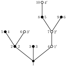
	$X^{1,1}$	$X^{1,2}$
	$X^{2,1}$	$X^{2,2}$

Figure 1. Multitype tree with 2 types and its breadth-first walk. We show type 1 individuals as filled circles, and type 2 individuals as empty circles. The breadth-first order of the (unitype) tree is depicted at the left of the vertices, and the breadth-first order of the subforests type 1 and type 2 are depicted at the right of the vertices, labeled by $1,2,3,4,5,6$ and $1^{\prime},2^{\prime},3^{\prime},4^{\prime}$ respectively.

The cyclical permutations that we use are the following. For $n\in\mathbb{N}$, consider any application $y:[n]_{0}\mapsto\mathbb{Z}^{d}$ with $y(0)=0$. The $n$-cyclical permutations of $y$ are the $n$ applications $\theta_{q,n}(y)$, for $q\in[n-1]_{0}$ given by

$$\theta_{q,n}(y)=\begin{cases}y(j+q)-y(q)&j\leq n-q\\ y(j+q-n)+y(n)-y(q)&n-q\leq j\leq n.\end{cases}$$

We say that the path $y:\mathbb{N}\mapsto\mathbb{Z}$ is a downward skip-free chain, if $y_{k+1}-y_{k}\in\mathbb{Z}_{+}\cup\{-1\}$. The possible paths that a coding of multitype forest can take are the following.

Definition.

Fix any ${\bf n}=(n_{1},\ldots,n_{d})\in\mathbb{Z}^{d}_{+}$, and define $S_{d}$ as the set of $[\mathbb{Z}^{d}]^{d}$-valued sequences $x=(x^{(1)},\ldots,x^{(d)})$ such that for all $i\in[d]$, $x^{(i)}=(x^{i,1},\ldots,x^{i,d})$ is a $\mathbb{Z}^{d}$-valued sequence starting at zero of length $n_{i}$, and where $x^{i,j}=(x^{i,j}_{k},k\in[n_{i}]_{0})$ is non-decreasing when $i\neq j$, and a downward skip-free chain when $i=j$.

The ${\bf n}$-cyclical permutations of $x\in S_{d}$ are given by

$$\theta_{{\bf q},{\bf n}}(x):=(\theta_{q_{1},n_{1}}(x^{(1)}),\ldots,\theta_{q_{d},n_{d}}(x^{(d)}))\ \ \ \ \ \ \ \ \ \forall\ {\bf q}=(q_{1},\ldots,q_{d})\mbox{ such that }0\leq{\bf q}\leq{\bf n}-1_{d},$$

with $1_{d}=(1,\ldots,1)$ of length $d$. Each sequence $\theta_{{\bf q},{\bf n}}(x)$ will be called a cyclical permutation of $x$.

For ${\bf m,n}\in\mathbb{Z}^{d}_{+}$, write ${\bf m}<{\bf n}$ if ${\bf m}\leq{\bf n}$ (the inequality understood component-wise) and if there exists $i$ such that $m_{i}<n_{i}$. Sequences $x\in S_{d}$ will be denoted by $x=(x^{i,j}_{k},k\in[n_{i}]_{0},i,j\in[d])$, and the vector ${\bf n}=(n_{1},\ldots,n_{d})\in\mathbb{Z}^{d}_{+}$, is called the length of $x$. Fix any such $x$ of length ${\bf n}$, and ${\bf r}=(r_{1},\ldots,r_{d})\in\mathbb{Z}^{d}_{+}$ with $\sum r_{i}>0$. We say that the system $({\bf r},x)$ admits a solution if there exists ${\bf m}\leq{\bf n}$ such that

(2) $$r_{j}+\sum_{i=1}^{d}x^{i,j}(m_{i})=0\ \ \ \ \ \ \ \forall\ j\in[d].$$

If there is no smaller solution ${\bf m}<{\bf n}$ for the system $({\bf r},{\bf\theta_{{\bf q},{\bf n}}}(x))$, then we call ${\bf\theta_{{\bf q},{\bf n}}}(x)$ a good cyclical permutation. It is proved in [CL16] that only such good cyclical permutations code multitype forests, and the next lemma tells us how many there are.

Lemma 1 (Multivariate Cyclic Lemma [CL16]).

Let $x\in S_{d}$ with $x^{i,i}(n_{i})\neq 0$ for every $i\in[d]$. Consider the system $({\bf r},x)$ with solution ${\bf n}$ as above. Then, the number of good cyclical permutations of $x$ is $det((-x^{i,j}(n_{i}))_{i,j\in[d]})$.

Since in most of the cases, we fix the number of roots or number of individuals of each type, we need the following definition.

Definition (Root-type and individuals-type).

We say a multitype plane forest with $d\in\mathbb{N}$ types has root-type ${\bf r}=(r_{1},\ldots,r_{d})\in\mathbb{N}^{d}$, if it has $r_{i}$ roots of type $i$ for $i\in[d]$, with ${\bf r}>0$ (that is, $r_{i}>0$ for some $i$). Also, it has individuals-type ${\bf n}=(n_{1},\ldots,n_{d})\in\mathbb{N}^{d}$ if it has $n_{i}$ individuals of type $i$, for $i\in[d]$.

1.1.2. Multitype Galton-Watson forests

Consider a (unitype) branching forest with $k$ trees and progeny distribution $\nu$ on $\mathbb{Z}_{+}$, that is, each of the $k$ individuals at generation 0 has offspring according to $\nu$, and each of its children has offspring independently of the others and with the same law. Such forests are also called GW forests. A multitype Galton-Watson (MGW) forest in $d$-types, is a branching forest, where each individual has a type $i\in[d]$, and has children independently of the others, according to a law $\nu_{i}$ on $\mathbb{Z}^{d}_{+}$. The progeny distribution of the forest is $\nu=(\nu_{1},\ldots,\nu_{d})$. The formal definition is the following.

Definition.

A multitype Galton-Watson process is a Markov chain $Z=\left(\left(Z_{n}^{(1)},\ldots,Z_{n}^{(d)}\right);n\geq 0\right)$ on $\mathbb{Z}^{d}_{+}$, with transition function

$$\mathbb{P}\!\left(Z_{n+1}=(k_{1},\ldots,k_{d})\,|Z_{n}=(r_{1},\ldots,r_{d})\right)=\nu_{1}^{*r_{1}}*\cdots*\nu_{d}^{*r_{d}}(k_{1},\ldots,k_{d}),$$

where $\nu$ is the progeny distribution, and $\nu_{i}^{*j}$ is the $j$th iteration of the convolution product of $\nu_{i}$ by itself, with $\nu_{i}^{*0}=\delta_{0}$.

For ${\bf r}\in\mathbb{Z}^{d}_{+}$, the probability measure $\mathbb{P}_{{\bf r}}$ is the law $\mathbb{P}\left(\cdot|Z_{0}={\bf r}\right)$. As in Theorem 1.2 in [CL16], we consider MGW trees satisfying the following. For $i,j\in[d]$, let $m_{i,j}=\sum_{z\in\mathbb{Z}_{+}^{d}}z_{j}\nu_{i}(z)$ be the mean number of children type $j$ given by an individual type $i$, and set $M=(m_{i,j})_{i,j}$ as the mean matrix of the MGW tree. Whenever $M$ is irreducible, by the Perron-Frobenius Theorem (see [AN04, Chapter V.2]), it has a unique eigenvalue which is simple, positive and with maximal modulus. We say in such case that the MGW tree is irreducible. If the unique eigenvalue equals one (is less than one), then we say the tree is critical (subcritical). The tree is non-degenerate if individuals have exactly one offspring with probability different from one.

1.2. Statement of the results

1.2.1. Multitype forests with a given degree sequence

To define uniform $d$-type forests with a given degree sequence, having root-type ${\bf r}>0$, we first define a multitype degree sequence. A multitype degree sequence ${\bf S}=({\bf S}_{i,j},i,j\in[d])$ is a sequence of sequences of non-negative integers ${\bf S}_{i,j}=(N_{i,j}(k);k\in[m_{i,j}]_{0})$, where $m_{i,j}\in\mathbb{N}$, satisfying:

1. $n_{i}=\sum_{k}N_{i,j}(k)$ for every $i,j\in[d]$, with $n_{i}>0$ for some $i$,

2. $n_{j}=r_{j}+\sum_{k}kN_{1,j}(k)+\cdots+\sum_{k}kN_{d,j}(k)$, for every $j\in[d]$, with $0\leq r_{i}\leq n_{i}$ for every $i$, and $r_{i}>0$ for some $i$,

3. $\det(-k_{i,j})>0$ with $k_{i,j}:=\sum kN_{i,j}(k)-n_{i}{\bf{1}}\left\{i=j\right\}$ and $k_{i,i}<0$ for every $i\in[d]$.

The value $N_{i,j}(k)$ represents the number of individuals of type $i$ with $k$ children of type $j$, so $n_{i}$ represents the total number of individuals of type $i$. Thus, the total number of vertices is $s:=n_{1}+\cdots+n_{d}=\sum_{k}N_{1,j}(k)+\cdots+\sum_{k}N_{d,j}(k)$ for $j\in[d]$. The last condition is imposed to obtain a forest with such degree sequence (see page 3). For simplicity, we will assume that our multitype degree sequences satisfy the third condition and we focus on the first two conditions. Table 1 summarizes the case $d=2$. More explicitly, the tree in Figure 1 has multitype degree sequence ${\bf S}_{1,1}=(4,1,1)$, ${\bf S}_{1,2}=(3,3)$, ${\bf S}_{2,1}=(3,0,1)$ and ${\bf S}_{2,2}=(3,1)$.

${\bf S}_{1,1}=(N_{1,1}(0),\ldots,N_{1,1}(m_{1,1}))$	${\bf S}_{1,2}=(N_{1,2}(0),\ldots,N_{1,2}(m_{1,2}))$	$n_{1}=\sum_{k}N_{1,j}(k)$
${\bf S}_{2,1}=(N_{2,1}(0),\ldots,N_{2,1}(m_{2,1}))$	${\bf S}_{2,2}=(N_{2,2}(0),\ldots,N_{2,2}(m_{2,2}))$	$n_{2}=\sum_{k}N_{2,j}(k)$
$n_{1}=r_{1}+\sum_{k}kN_{1,1}(k)+kN_{2,1}(k)$	$n_{2}=r_{2}+\sum_{k}kN_{1,2}(k)+kN_{2,2}(k)$	$n_{1}+n_{2}=s$

Table 1. Relations on the degree sequence of a 2-type forest.

As in the unitype case, we construct the canonical child sequence ${\bf c}=({\bf c}_{i,j},i,j\in[d])$ from the degree sequence, that is, let ${\bf c}_{i,j}$ be a sequence whose first $N_{i,j}(0)$ entries are zeros, the next $N_{i,j}(1)$ entries are ones, and so on. Let $\sigma_{i,j}$ be any permutation on $[n_{i}]$, and construct $w^{b}=\{w^{b}_{i,j};i,j\in[d]\}$, where

$$w^{b}_{i,j}(k)=\sum_{l=1}^{k}\left({\bf c}_{i,j}\circ\sigma_{i,j}(l)-{\bf{1}}\left\{i=j\right\}\right),\ \ \ \ k\in[n_{i}].$$

Remark 1.

Note that $k_{i,j}:=w^{b}_{i,j}(n_{i})$ does not depend on the permutation, so it is deterministic. Also, note that the system of equations $({\bf r},w^{b})$ admits ${\bf n}$ as a solution, since by definition

$$r_{j}+\sum_{i=1}^{d}w^{b}_{i,j}(n_{i})=r_{j}-n_{j}+\sum_{i=1}^{d}\sum kN_{i,j}(k)=0\ \ \ \ \ \ \ \ \forall\,j\in[d].$$

Finally, note that $-k_{j,j}=r_{j}+\sum_{i\neq j}k_{i,j}$ since by definition, we have

$$-k_{j,j}=n_{j}-\sum_{k}kN_{j,j}(k)=r_{j}+\sum_{i}\sum_{k}kN_{i,j}(k)-\sum_{k}kN_{j,j}(k)=r_{j}+\sum_{i\neq j}k_{i,j}.$$

Trivially, whenever $r_{j}>0$ we have $-k_{j,j}>0$.

From the Multivariate Cyclic Lemma 1, we know that $\det(-k_{i,j})$ is the number of good cyclical permutations of $w^{b}$, considering the system $({\bf r},w^{b})$. We define a Vervaat-type transformation of $w^{b}$, given by choosing uniformly at random a good-cyclical permutation from all the good-cyclical permutations. After that, the algorithm is similar to the unidimensional case.

Definition (Multidimensional Vervaat Transform).

Fix any $w^{b}$ as constructed above, with corresponding ${\bf r}$ and any $u\in[\det(-k_{i,j})]$. Define $V(w^{b},u)$ as follows: enumerate the $\det(-k_{i,j})$ good cyclical permutations of $w^{b}$, using the lexicographic order on the set of ${\bf q}$ such that $\theta_{{\bf q,n}}(w^{b})$ codes a forest; then, let $V(w^{b},u)$ be the $u$-th good cyclical permutation.

Let $\mathbb{F}_{{\bf r,S}}$ be the set of multitype plane forests with degree sequence ${\bf S}$, having root-type ${\bf r}$ and individuals-type ${\bf n}$. Let $W=(W_{i,j},i,j\in[d])$ be a random process taking values on $S_{d}$. Then, we denote by $\mathbb{P}_{{\bf r}}$ the law in which each $W_{i,j}$ starts at $W_{i,j}(0)=r_{i}{\bf{1}}\left\{i=j\right\}$.

The next result gives us a simple way to obtain the BFW (as constructed in (1)) of a MFGDS (the proof is given on page 3).

Theorem 1 (Uniform multitype forest with a given degree sequence).

Fix the degree sequence ${\bf S}$ of a multitype forest having root-type ${\bf r}$ and individuals-type ${\bf n}$. Let ${\bf W}$ be the BFW coding a forest taken uniformly at random from $\mathbb{F}_{{\bf r,S}}$. Let ${\bf\pi}=(\pi_{i,j},i,j\in[d])$ be independent random permutations, where $\pi_{i,j}$ takes values on $[n_{i}]$, and let $U$ be an independent uniform variable on $[\det(-k_{i,j})]$. Define the processes ${\bf W}^{b}=(W^{b}_{i,j},i,j\in[d])$ as

$$W^{b}_{i,j}(k)=\sum_{l=1}^{k}({\bf c}_{i,j}\circ\pi_{i,j}(l)-{\bf{1}}\left\{i=j\right\}),\ \ \ \ k\in[n_{i}],$$

where ${\bf c}=\left(c_{i,j},i,j\in[d]\right)$ is the child sequence of ${\bf S}$. Then

$$V({\bf W}^{b},U)\stackrel{{\scriptstyle d}}{{=}}{\bf W},$$

under the law $\mathbb{P}_{{\bf r}}$ and the uniform law on $\mathbb{F}_{{\bf r,S}}$, respectively.

From the proof, we obtain $|\mathbb{F}_{{\bf r,S}}|$, the number of multitype forests with a given degree sequence ${\bf S}$ (cf. Theorem 3.3.2 in [Ngu16])

$$|\mathbb{F}_{{\bf r,S}}|=\frac{\det(-k_{i,j})}{\prod n_{i}}\prod\prod{n_{i}\choose{\bf S}_{i,j}}.$$

In Figures 2 and 3 we depict two simulations of MFGDS.

Figure 2. MFGDS with three types, having 8 000 vertices.

Figure 3. MFGDS with three types, having 32 000 vertices.

1.2.2. MGW forests conditioned by types

Before turning to the joint law of the number of individuals of type $i\in[d]$, of a MGW forest, we prove that the latter model is a mixture of MFGDS in Section 4. This justifies the importance of MFGDS.

Let $X=(X^{(1)},\ldots,X^{(d)})$ be $d$ random walks on $\mathbb{Z}^{d}$, where

(3) $$\mathbb{P}\!\left(X^{(i)}_{1}={\bf k}\right)=\nu_{i}({\bf k}+{\bf e}_{i}),$$

${\bf k}$ is a vector with entries in $\mathbb{Z}_{+}$ except at position $i$, which takes values on $\mathbb{Z}_{+}\cup\{-1\}$, and ${\bf e}_{i}$ is the vector with zeros except a one at position $i$. We will write $X^{(i)}=(X^{i,1},\ldots,X^{{i,d}})$. Our hypotheses are the following:

H1:

For every $i\in[d]$, the law $\nu_{i}$ has independent components, that is

$$\nu_{i}^{*n_{i}}\left({\bf k}+{\bf e}_{i}\right)=\prod_{j}\mathbb{P}\!\left(X^{i,j}_{n_{i}}=k_{j}\right)\ \ \ \ \ \ {\bf k}=(k_{1},\ldots,k_{d}),k_{j}\in\mathbb{Z}_{+}\mbox{ for $j\neq i$ and }k_{i}\in\mathbb{Z}_{+}\cup\{-1\}.$$

H2:

For every $i,j\in[d]$, with $i\neq j$

$$\mathbb{E}\!\left(X^{i,j}_{n_{i}};\sum_{l\in[d]}X^{l,j}_{n_{l}}=n_{j}-r_{j}\right)=\frac{n_{i}(n_{j}-r_{j})}{n}\mathbb{P}\!\left(\sum_{l\in[d]}X^{l,j}_{n_{l}}=n_{j}-r_{j}\right).$$

It is important to remark that we do not assume that the components $\nu_{i}$ have the same distribution. The following result (see page 5 for the proof) is a generalization of the Otter-Dwass formula [Ott49, Dwa69] (Lemma 3.8 in [ADG18] also gives a formula for the joint law of the sizes of a MGW forest, but less explicit).

Theorem 2.

Consider an irreducible, non-degenerate and (sub)critical MGW forest, and let $n_{i}>0$ for every $i$ and ${\bf r}>0$. Suppose that ${\bf H1}$ and ${\bf H2}$ and are also satisfied. If $O_{i}$ is the number of type $i$ individuals, then

$$\mathbb{P}_{{\bf r}}\left(O_{i}=n_{i},i\in[d]\right)=\frac{r}{n}\prod_{i=1}^{d}\mathbb{P}\!\left(\sum_{l\in[d]}X^{l,i}_{n_{l}}=n_{i}-r_{i}\right),$$

where $r=r_{1}+\cdots+r_{d}$ and $n=n_{1}+\cdots+n_{d}$, and $r_{i}<n_{i}$.

Remark 2.

Under the assumption $n_{i}>0$ for every $i$, the proof is simpler, but we think this hypothesis can be dropped as in [CL16].

Remark 3.

On page 7, we obtain the case when $n_{i}=r_{i}$ for some $i$’s. Since Theorem 2 has a different formula on such case, the law of $\sum_{i\in[d]}O_{i}$ (computed on Corolary 1) does not have a nice expression.

For the next results denote by $\mathbb{F}^{plane}_{{\bf r,n}}$, $\mathbb{F}^{labeled}_{{\bf r,n}}$ and $\mathbb{F}^{binary}_{{\bf r,n}}$, the set of $d$-type plane, labeled and binary forests having root-type ${\bf r}$ and individuals-type ${\bf n}$, where $r_{i}<n_{i}$ for every $i$ and ${\bf r}>0$. Our labeled multitype forests have labels on $[n]$, that is, for $F\in\mathbb{F}^{labeled}_{{\bf r,n}}$, each individual $v$ has a unique label $i\in[n]$ and a type $c_{F}(v)\in[d]$; also, $F$ has fixed root set $[r]$, that is, the $r_{1}$ type 1 roots have labels on $\{1,\ldots,r_{1}\}$, the $r_{2}$ type 2 roots have labels on $\{r_{1}+1,\ldots,r_{1}+r_{2}\}$, and so on. Using Theorem 2, we give in Subsection 5.1 three examples of distributions were the law of a MGW forest conditioned by the number of individuals of each type can be computed explicitly. This generalizes the constructions given in [Pit98].

Proposition 1.

For fixed $p\in(0,1)$, let $\mathcal{G}_{{\bf r},p}$ be a $d$-type GW forest with root-type ${\bf r}$, having geometric offspring distribution with parameter $p$ independently for each type, that is, $\nu_{i}(k_{1},\ldots,k_{d})=\prod_{i}p(1-p)^{k_{i}}$ for $k_{i}\geq 0$. Let $\#_{i}\mathcal{G}_{{\bf r},p}$ be the number of type $i$ individuals in $\mathcal{G}_{{\bf r},p}$. Then

$$\mathbb{P}\!\left(\mathcal{G}_{{\bf r},p}=F|\#_{i}\mathcal{G}_{{\bf r},p}=n_{i},i\in[d]\right)=\frac{1}{\frac{r}{n}\prod_{i\in[d]}{n+n_{i}-r_{i}-1\choose n_{i}-r_{i}}}\ \ \ \ \ \ \forall\,F\in\mathbb{F}^{plane}_{{\bf r},{\bf n}},$$

thus, such conditioned forest is uniform on $\mathbb{F}^{plane}_{{\bf r,n}}$.

Proposition 2.

For $\mu\in\mathbb{R}^{+}$, let $\mathcal{P}_{{\bf r},\mu}$ be a $d$-type GW forest with root-type ${\bf r}$, having Poisson offspring distribution of parameter $\mu$ independently for each type, that is, $\nu_{i}(k_{1},\ldots,k_{d})=\prod_{i}e^{-\mu}\mu^{k_{i}}/k_{i}!$ for $k_{i}\geq 0$. Let $\#_{i}\mathcal{P}_{{\bf r},p}$ be the number of type $i$ individuals in $\mathcal{P}_{{\bf r},p}$. If $\mathcal{P}^{*}_{{\bf r,n}}$ is $\mathcal{P}_{{\bf r,n}}$ relabeled by $d$ uniform random permutations, one for each type, then

$$\mathbb{P}\!\left(\mathcal{P}_{{\bf r},p}^{*}=F|\#_{i}\mathcal{P}_{{\bf r},p}=n_{i},i\in[d]\right)=\frac{1}{\frac{r}{n}n^{n-r}}\ \ \ \ \ \ \forall\,F\in\mathbb{F}^{labeled}_{{\bf r},{\bf n}},$$

thus, such conditioned forest is uniform on $\mathbb{F}^{labeled}_{{\bf r,n}}$.

Proposition 3.

For $0<p<1$, let $\mathcal{B}_{{\bf r},p}$ be a $d$-type GW forest with root-type ${\bf r}$, having Bernoulli offspring distribution with parameter $p$, for each vertex independently of the type, that is, $\nu_{i}(k_{1},\ldots,k_{d})=\prod p^{k_{i}}(1-p)^{1-k_{i}}$ with $k_{i}\in\{0,1\}$. Assume that $n_{i}-r_{i}$ is an even number for every $i\in[d]$. Since any vertex $v$ has zero or two children with probability $p$ or $1-p$ respectively, then $\nu_{i}(c_{1}(v),\ldots,c_{d}(v))=\prod p^{c_{i}(v)/2}(1-p)^{1-c_{i}(v)/2}$. Let $\#_{i}\mathcal{B}_{{\bf r},p}$ be the number of type $i$ individuals in $\mathcal{B}_{{\bf r},p}$. Then

$$\mathbb{P}\!\left(\mathcal{B}_{{\bf r},p}=F|\#_{i}\mathcal{B}_{{\bf r},p}=n_{i},i\in[d]\right)=\frac{1}{\frac{r}{n}\prod{n\choose(n_{i}-r_{i})/2}}\ \ \ \ \ \ \forall\,F\in\mathbb{F}^{binary}_{{\bf r},{\bf n}},$$

thus, such conditioned forest is uniform on $\mathbb{F}^{binary}_{{\bf r,n}}$.

As a simple consequence of our results, we obtain the following enumerations.

Lemma 2.

The number of $d$-type plane, labeled, and binary forest, with root-type ${\bf r}$ and individuals-type ${\bf n}$ is given respectively by

$$\frac{r}{n}\prod_{i\in[d]}{n+n_{i}-r_{i}-1\choose n_{i}-r_{i}},\ \ \ \ \ \frac{r}{n}n^{n-r}\ \ \ \mbox{and}\ \ \ \frac{r}{n}\prod{n\choose(n_{i}-r_{i})/2}.$$

Finally, we give an algorithm to simulate MGW processes conditioned by its types. This is done using the following proposition and an Accept-Reject method (see Algorithm 9).

Proposition 4.

Let $W$ be the BFW of a CMGW(${\bf n}$) forest satisfying the Hypotheses of Theorem 2, having offspring distribution $\nu$, and root-type ${\bf r}$, with $0<r_{i}<n_{i}$ for every $i$. Generate independent multinomial vectors ${\bf S}_{i,j}=(N_{i,j}(0),N_{i,j}(1),\ldots)$ with parameters $(n_{i},\nu_{i,j}(0),\nu_{i,j}(1),\ldots)$, and stop the first time that $r_{j}+\sum_{i}\sum_{k}kN_{i,j}(k)=n_{j}$ for every $j$. Denote by ${\bf S}$ the multitype degree sequence obtained, and let $V({\bf W}^{b},U)$ be the BFW generated by Theorem 1 using the degree sequence ${\bf S}$. Then,

$$\mathbb{P}_{{\bf r}}\left(V({\bf W}^{b},U)=w\right)=\frac{1}{\frac{n}{r}\frac{\det(-k_{i,j})}{\prod n_{i}}}\mathbb{P}_{{\bf r}}\left(\mathcal{F}=F|\#_{j}\mathcal{F}=n_{j},\forall\ j\right),$$

for every multitype forest $F$ coded by $w$, with root-type ${\bf r}$, individuals-type ${\bf n}$, multitype degree sequence $(n_{i,j},i,j\in[d])$ and with $k_{i,j}=\sum kn_{i,j}(k)-n_{i}{\bf{1}}\left\{i=j\right\}$.

The paper is organized as follows: in Section 2 we construct uniform unitype forests with a given degree sequence. This will be used in Section 3, to construct MFGDS and prove Theorem 1. In Section 4 we prove that under an independence assumption, the CMGW forests are mixtures of MFGDS. Section 5 is devoted to prove the joint law of the number of individuals by types in a MGW forest, which is Theorem 2. In that section we also obtain in Corollary 1, the law of the total population in a MGW forest. Examples satisfying the hypotheses of Theorem 2 are given in Subsection 5.1. The algorithms are given in Section 6.

2. Construction of unitype random forests with a given degree sequence

A well-known encoding of forests by skip-free random walks is given as follows. Define the set of all bridges finishing in position $-m$ at time $s$, as

$$\mathbb{B}^{s,m}=\left\{(y(1),\ldots,y(s))\in\mathbb{Z}^{s}:y(j)-y(j-1)\geq-1\mbox{ for $j\in[s]$},y(s)=-m\right\}.$$

For $i\in[s]-1$ and $y\in\mathbb{B}^{s,m}$, define $\theta_{i}(y)$ as the cyclic permutation of $y$ at $i$, that is

$$(\theta_{i}(y))(j)=\begin{cases}y(j+i)-y(i)&j+i\leq s\\ y(j+i-s)+y(s)-y(i)&s-i\leq j\leq s.\end{cases}$$

This transformation puts the last $s-i$ increments of $y$ as the first $s-i$ increments of $\theta_{i}(y)$, and the first $i$ increments of $y$ as the last $i$ increments of $\theta_{i}(y)$.

For any $u\in[m]-1$ and $y\in\mathbb{B}^{s,m}$, let $\tau_{u}$ be the time that $y$ hits $min(y)+u$ for the first time. The Vervaat-type transformation $V$ that we use is given by

$$V(y,u)=\theta_{\tau_{u}}(y).$$

Note that this transformation leads the set of bridges, to the set of excursions of size $s$ finishing at $-m$

$$\mathbb{E}^{s,m}=\left\{(w(1),\ldots,w(s))\in\mathbb{Z}^{s}:w(j)-w(j-1)\in\{-1,0,1,\ldots\}\mbox{ for $j\in[s]$, $w$ first reaches $-m$ at time $s$}\right\}.$$

Now, let $F$ be a forest with trees $T_{1},\ldots,T_{m}$, for $m\in\mathbb{N}$. The degree sequence of $F$ is given by

$$N_{i}(F)=\sum_{1}^{m}N_{i}(T_{j}).$$

Note that, any finite sequence of non-negative integers ${\bf S}=(N_{i},i\geq 0)$, such that for some $m\in[|{\bf S}|]$, we have

$$s:=\sum N_{i}=\sum iN_{i}+m,$$

is the degree sequence of some forest with $m$ trees. In this case we call ${\bf S}$ a degree sequence. The size of the forest $F$ will also be denoted by $|F|$.

Fix any degree sequence ${\bf S}$ and obtain its child sequence ${\bf c}:={\bf c(S)}$. As before, we obtain an EI process using uniform permutations of the child sequence ${\bf c}$. Let $\sigma$ be any permutation on $[s]$. Define the bridge

$$w^{b}(j)=\sum_{1}^{j}(c\circ\sigma(i)-1)\ \ \ \ \ j\in[s],$$

with $w^{b}(0)=0$. Note that $w^{b}(s)=-m$. The set of paths taken by $w^{b}$ is

$$\mathbb{B}_{{\bf S}}=\left\{(y(1),\ldots,y(s))\in\mathbb{B}^{s,m}:|j:y(j)-y(j-1)=i-1|=N_{i}\mbox{ for every $i\geq 0$}\right\}.$$

From the excursions in $\mathbb{E}^{s,m}$, we consider those with fixed number of increments of given size:

$$\mathbb{E}_{{\bf S}}=\left\{(w(1),\ldots,w(s))\in\mathbb{E}^{s,m}:|j:w(j)-w(j-1)=i-1|=N_{i},i\geq 0\right\}.$$

Define $\mathbb{F_{{\bf S}}}$ as the set of all forests with degree sequence ${\bf S}$. Using Lemma 6.3 of [Pit06], it can be proved that there exists a bijection between $\mathbb{E}_{{\bf S}}$ and $\mathbb{F}_{{\bf S}}$, and we know that $|\mathbb{F}_{{\bf S}}|=\frac{m}{s}{s\choose N_{i},i\geq 0}$.

It is clear from a picture, that a bridge is sent to an excursion by the Vervaat transformation. Let us prove this is also the case for bridges in $\mathbb{B}_{{\bf S}}$, that is, bridges coming from a degree sequence ${\bf S}$. The next three lemmas are inspired in [Lei19].

Lemma 3.

For any $u\in[m]-1$ and $y\in\mathbb{B}_{{\bf S}}$, the path $V(y,u)$ belongs to $\mathbb{E}_{{\bf S}}$.

Proof.

By definition of $\tau_{u}$, the minimum value that can take $y(\tau_{u}+j)-y(\tau_{u})$ for $j+\tau_{u}\leq s$ is $-u>-m$. These are the first $s-\tau_{u}$ times of $V(y,u)$. On the remaining times $\{s-\tau_{u},\ldots,s\}$, the minimum of $V(y,u)$ is attained for the first time at time $s$. This implies $V(y,u)(j)>-m$ for $j<s$, and hence $V(y,u)\in\mathbb{E}$. Since the Vervaat transformation only permutes the increments, it is clear that if $y\in\mathbb{B}_{{\bf S}}$ then $V(y,u)\in\mathbb{E}_{{\bf S}}$. ∎

Lemma 4.

Let $w\in\mathbb{E}_{{\bf S}}$. Then, the number of different pairs $(y,u)\in\mathbb{B}_{{\bf S}}\times([m]-1)$ such that $V(y,u)=w$ is exactly $s$.

Proof.

Consider any $i\in[s]-1$ and the cyclical permutation $y^{\prime}=\theta_{i}(w)$. It is clear that $\theta_{s-i}(y^{\prime})=w$. In fact $V(y^{\prime},u)=w$ for some $u\in[m]-1$. This holds true since the last $s-i$ increments of $w$ are the first $s-i$ increments of $y^{\prime}$, then $y^{\prime}$ hits $y^{\prime}(s-i)=w(s)-w(s-i)$ for the first time at time $s-i$. Hence, the Vervaat transform can be applied at $u=y^{\prime}(s-i)$, giving us the path $w$.

Note that the path of $w$ can be partitioned in $m$ subexcursions, each one of the form $(w(j+T_{i}),j\in[T_{i+1}-T_{i}])$, with $i\in[m]-1$ and $T_{i}$ the first hitting time to $-i$. First assume that $w$ can be partitioned in $k_{w}\in[m]$ identical subexcursions, each of length $l_{w}$. It follows $k_{w}l_{w}=s$. This is equivalent to say that there exists $k_{w}$ values $u$ such that $V(w,u)=w$. Those values are $w(jl_{w})+m\in[m]-1$ for $j\in[k_{w}]$. In this case, there are only $l_{w}$ different cyclic permutations $\theta_{i}(w)$ of $w$, each one having $k_{w}$ distinct values of $u$ such that $V(\theta_{i}(w),u)=w$. This proves that $w$ has exactly $s$ preimages. If $w$ cannot be partitioned in identical subexcursions, for every cyclical permutation $\theta_{i}(w)$ there is only one $u$ such that $V(\theta_{i}(w),u)=w$. This concludes the proof. ∎

Now, we construct a uniform forest on $\mathbb{F}_{{\bf S}}$.

Lemma 5.

Consider a degree sequence ${\bf S}$ of a forest having $m$ trees and $s$ individuals, and let $\mathcal{F}$ be a forest taken uniformly at random from $\mathbb{F}_{{\bf S}}$. Let $\pi$ be a uniform random permutation on $[s]$, $U$ an independent uniform variable on $[m]-1$, and define the bridge

$$W^{b}(j)=\sum_{1}^{j}(c\circ\pi(j)-1)\ \ \ \ \ \ \ \ j\in[s],$$

where ${\bf c}$ is the child sequence of ${\bf S}$. Then

$$V(W^{b},U)\stackrel{{\scriptstyle d}}{{=}}\mathcal{F},$$

under the law $\mathbb{P}_{m}$ that makes $W^{b}$ start at $m$ and the uniform law on $\mathbb{F}_{{\bf S}}$.

Proof.

Fix any $w\in\mathcal{E}_{\bf S}$ and any of its cyclical permutations $w^{b}\in\mathcal{B}_{\bf S}$. From the $s!$ possible values that $\pi$ can take, only $\prod N_{i}!$ give the same bridge $w^{b}$. This is true since we can permute the labels of the $N_{i}$ individuals having $i$ children and obtain the same bridge. Hence

$$\mathbb{P}_{m}\left(W^{b}=w^{b}\right)=\frac{1}{{s\choose N_{i},i\geq 0}},$$

which does not depend on $w^{b}$.

By the previous lemma, there are $s$ distinct pairs $(w^{b},u)$ that are mapped to $w$. Denote such pairs as $(w^{b}_{k},u_{k})\in\mathcal{B}_{\bf S}$, for $k\in[s]$. Then, using the independence of $W^{b}$ and $U$, and that the former is uniform, then

$$\mathbb{P}_{m}\left(V(W^{b},U)=w\right)=\sum_{k=1}^{s}\mathbb{P}_{m}\left(W^{b}=w^{b}_{k},U=u_{k}\right)=\frac{s}{m}\mathbb{P}_{m}\left(W^{b}=w^{b}\right)=\frac{1}{|\mathbb{F}_{{\bf S}}|}.\qed$$

3. Construction of multitype random forests with a given degree sequence

Recall that from a given multitype degree sequence, we can construct bridges $w^{b}$ taking values on $S_{d}$ such as before the remark 1, together with its multidimensional Vervaat transform $V(w^{b},u)$ Definition. The set of possible paths of $w^{b}$ constructed in this manner, will be denoted by $\mathbb{B}_{{\bf r,S}}$. Explicitly, this is the set of $d\times d$ bridges $(w^{b}_{i,j},i,j\in[d])$ in $S_{d}$, where $w^{b}_{i,j}$ finishes at $k_{i,j}=\sum kN_{i,j}(k)-n_{i}{\bf{1}}\left\{i=j\right\}$, and with $N_{i,j}(k)$ increments of size $k-1$, for each $i,j\in[d]$ and $k$. The set of plane forests with degree sequence ${\bf S}$ having root-type ${\bf r}$, will be denoted by $\mathbb{F}_{{\bf r,S}}$, and the set of BFWs coding such forests by $\mathbb{E}_{{\bf r,S}}$. Now we are ready to construct a forest taken uniformly at random from $\mathbb{F}_{{\bf r,S}}$.

Proof of Theorem 1.

First we prove that from any multitype degree sequence, we can construct a multitype forest. From Remark 1, we can associate to the degree sequence a system of equations $({\bf r},w^{b})$ with solution ${\bf n}$. To such system we can associate a multitype forest using the Multivariate Cyclic Lemma 1 (note that $k_{i,i}<0$ by definition of multitype degree sequence), since any good cyclical permutation codes a forest.

Now, define ${\bf S}_{i,j}=(N_{i,j}(k);k\geq 0)$, and write

$${n_{i}\choose{\bf S}_{i,j}}:={n_{i}\choose N_{i,j}(0),N_{i,j}(1),\ldots}.$$

Fix any bridge $w^{b}\in\mathbb{B}_{{\bf r,S}}$. From the possible $\prod_{i}(n_{i}!)^{d}$ values taken by the random permutations $({\bf\pi}_{i,j},i,j\in[d])$, exactly $\prod_{j}\prod_{i}\prod_{k}N_{i,j}(k)!$ form the bridge $w^{b}$. This is true since, permuting the labels of the $N_{i,j}(k)$ individuals type $i$ having $k$ children type $j$, we obtain the same bridge. This proves the assertion since this is true for every $i,j,k$. Therefore

$$\mathbb{P}_{{\bf r}}\left({\bf W}^{b}=w^{b}\right)=\frac{1}{\prod\prod{n_{i}\choose{\bf S}_{i,j}}}.$$

Now, fix any $w\in\mathbb{E}_{{\bf r,S}}$ and $i\in[d]$. We obtain the number of different pairs $(w^{b},u)$ that can be mapped to $w$ using the multidimensional Vervaat transform. The point is that such bridges can only be of the form $\theta_{{\bf q,n}}(w)$, that is, cyclical permutations of $w$. Hence, each component $w^{(i)}$ comes from a Vervaat transform $V(\theta_{j}(w^{(i)}),u)$ for some $j,u$. By Lemma 4, the number of pairs $(\theta_{j}(w^{(i)}),u)$ that can be mapped to $w^{(i)}$ are exactly $n_{i}$. This being true for every $i$ implies there are $\prod n_{i}$ unique pairs $(\theta_{\bf q,n}(w),u)$ such that $V((\theta_{\bf q,n}(w),u))=w$. Denote such pairs as

$$A(w)=\left\{(w^{b}_{k},u_{k})\in\mathbb{B}_{{\bf r,S}}\times[\det(-k_{i,j})]:V((w^{b}_{k},u_{k}))=w,k\in\left[\prod n_{i}\right]\right\}.$$

This implies

$$\mathbb{P}_{{\bf r}}\left(V({\bf W}^{b},U)=w\right) =\mathbb{P}_{{\bf r}}\left(({\bf W}^{b},U)\in A(w)\right)$$

$$=\sum_{k\in\left[\prod n_{i}\right]}\mathbb{P}_{{\bf r}}\left(({\bf W}^{b},U)=(w^{b}_{k},u_{k})\right)$$

$$=\sum_{k\in\left[\prod n_{i}\right]}\frac{1}{\prod\prod{n_{i}\choose{\bf S}_{i,j}}}\frac{1}{\det(-k_{i,j})}$$

$$=\frac{1}{\frac{\det(-k_{i,j})}{\prod n_{i}}\prod\prod{n_{i}\choose{\bf S}_{i,j}}}.$$

This concludes the proof since the right-hand side is independent of $w$, so $V({\bf W}^{b},U)$ is uniform. ∎

Remark 4.

From this lemma we can conclude that the set of plane forests with degree sequence ${\bf S}$ having root-type ${\bf r}$ is

$$|\mathbb{F}_{{\bf r,S}}|=\frac{\det(-k_{i,j})}{\prod n_{i}}\prod\prod{n_{i}\choose{\bf S}_{i,j}}.$$

4. Relation between MFGDS and CMGW forests

Before turning to the results about conditioned MGW forests, let us prove that under an independence condition, a MGW conditioned by its degree sequence has the same law as a MFGDS. For any given ${\bf n}=(n_{1},\ldots,n_{d})\in\mathbb{Z}_{+}^{d}$ and ${\bf r}=(r_{1},\ldots,r_{d})\in\mathbb{Z}_{+}^{d}$ with $\sum r_{i}>0$, define the set of all degree sequences having $n_{i}$ individuals of type $i$, as

$$DS({\bf r,n})= \left\{{\bf S}=(N_{i,j}(k),i,j\in[d],k\geq 0):\right.$$

$$\ \ \ \ \left.n_{i}=\sum_{k}N_{i,j}(k),\ n_{j}=r_{j}+\sum_{i}\sum_{k}kN_{i,j}(k),N_{i,j}(k)\geq 0\mbox{ for $i,j\in[d]$}\right\}.$$

Also, for any given multitype forest $F$, define its empirical multitype degree sequence $\hat{N}(F):=\hat{N}=(\hat{N}_{i,j}(k),i,j\in[d],k\geq 0)$ as

$$\hat{N}_{i,j}(k)=\sum_{l:v_{l}\in F^{(i)}}{\bf{1}}\left\{{\bf c}_{i,j}(l)=k\right\},$$

where the product is taken over all vertices of subforest $F^{(i)}$, and ${\bf c}_{i,j}(l)$ is the number of children type $j$, that the $l$th individual of the subforest $F^{(i)}$ of vertices type $i$ has.

Lemma 6.

Fix any ${\bf n}=(n_{1},\ldots,n_{d})\in\mathbb{Z}_{+}^{d}$ and ${\bf r}=(r_{1},\ldots,r_{d})\in\mathbb{Z}_{+}^{d}$ with $\sum r_{i}>0$. Consider a multitype degree sequence ${\bf S}=(N_{i,j}(k),i,j\in[d],k\geq 0)\in DS({\bf r,n})$. Consider a MGW forest with progeny distribution $\nu=(\nu_{1},\ldots,\nu_{d})$ such that each $\nu_{i}$ has independent components. Then, the law of a MGW forest conditioned to have multitype degree sequence ${\bf S}$ is the same as $\mathbb{P}_{{\bf S}}$, the law of a MFGDS. Also, the law of a CMGW(${\bf n}$) forest is a finite mixture of the laws $(\mathbb{P}_{{\bf S}},{\bf S}\in DS({\bf r,n}))$.

Proof.

Let $\mathcal{F}$ be a MGW tree. By the assumption on $\nu_{i}$, we can write $\nu_{i}({\bf z})=\prod_{j}\nu_{i,j}(z_{j})$ for any $z=(z_{1},\ldots,z_{d})\in\mathbb{Z}_{+}^{d}$, any $i$, and some laws $\nu_{i,j}$ on $\mathbb{Z}_{+}$. Let $(F_{1},c(F_{1}))$ and $(F_{2},c(F_{2}))$ be two multitype forests having degree sequence ${\bf S}\in DS({\bf r,n})$. Then

$$\mathbb{P}_{{\bf r}}\left(\mathcal{F}=F_{1},\hat{N}(\mathcal{F})={\bf S}\right) =\prod_{i}\prod_{k:v_{k}\in F_{1}^{(i)}}\prod_{j}\nu_{i,j}(c_{i,j}(k))$$

$$=\prod_{i}\prod_{j}\prod_{k}\nu_{i,j}(k)^{N_{i,j}(k)}$$

$$=\prod_{i}\prod_{k:v_{k}\in F_{2}^{(i)}}\prod_{j}\nu_{i,j}(c_{i,j}(k))$$

$$=\mathbb{P}_{{\bf r}}\left(\mathcal{F}=F_{2},\hat{N}(\mathcal{F})={\bf S}\right).$$

This implies the first assertion. Let ${\bf O}=(O_{1},\ldots,O_{d})$ be the vector with the total number of individuals of each type in a MGW forest. To prove the second assertion, we sum over all the values in $DS({\bf r,n})$, obtaining

$$\mathbb{P}_{{\bf r}}\left(\mathcal{F}\in\cdot|{\bf O}={\bf n}\right) =\frac{1}{\mathbb{P}_{{\bf r}}\left({\bf O}={\bf n}\right)}\sum_{{\bf S}\in DS({\bf r,n})}\mathbb{P}_{{\bf r}}\left(\mathcal{F}\in\cdot,\hat{N}(\mathcal{F})={\bf S}\right)$$

$$=\sum_{{\bf S}\in DS({\bf r,n})}\frac{\mathbb{P}_{{\bf r}}\left(\hat{N}(\mathcal{F})={\bf S},{\bf O}={\bf n}\right)}{\mathbb{P}_{{\bf r}}\left({\bf O}={\bf n}\right)}\mathbb{P}_{{\bf r}}\left(\mathcal{F}\in\cdot|\hat{N}(\mathcal{F})={\bf S}\right)$$

$$=\sum_{{\bf S}\in DS({\bf r,n})}\lambda_{{\bf S}}\mathbb{P}_{{\bf S}}\left(\mathcal{F}\in\cdot\right),$$

where

$$\lambda_{{\bf S}}=\mathbb{P}_{{\bf r}}\left(\hat{N}(\mathcal{F})={\bf S}|{\bf O}={\bf n}\right).$$

Note that trivially $\sum_{{\bf S}\in DS({\bf r,n})}\lambda_{\bf S}=1$. ∎

5. Law of the number of individuals by types of a MGW forest

The main result in [CL16] is the following.

Theorem 3 (Theorem 1.2, [CL16]).

Let $Z$ be a $d$-type branching process, which is irreducible, non-degenerate and (sub)critical. For $i\in[d]$, let $O_{i}$ be the total number of individuals of type $i$, up to the extinction time $T$, and for $i\neq j$, let $A_{i,j}$ be the total number of individuals of type $j$ whose parent is of type $i$, up to time $T$. Then, for all integers $r_{i}$, $n_{i}$, $k_{i,j}$ such that $r_{i}\geq 0$ with ${\bf r}>0$, $k_{i,j}\geq 0$ for $i\neq j$, $-k_{j,j}=r_{j}+\sum_{i\neq j}k_{i,j}$, and $n_{i}\geq-k_{i,i}$, we have

(4) $$\begin{split}&\mathbb{P}_{{\bf r}}\left(O_{i}=n_{i},i\in[d],A_{ij}=k_{ij},i,j\in[d],i\neq j\right)\\ &=\frac{det(-k_{ij})}{\bar{n}_{1}\cdots\bar{n}_{d}}\prod_{1}^{d}\nu_{i}^{*n_{i}}\left(k_{i1},\ldots,k_{i(i-1)},n_{i}+k_{ii},k_{i(i+1)},\ldots,k_{id}\right),\end{split}$$

where ${{\bf r}}=(r_{1},\ldots,r_{d})$, $\bar{n}_{i}=n_{i}\vee 1$ and $(-k_{ij})_{i,j\in[d]}$ is the matrix to which we remove row $i$ and column $i$, for every $i$ such that $n_{i}=0$.

For simplicity, we use $n_{i}>0$ for $i\in[d]$ in the following. Let us give a hint on how to derive the law of the population by types for a 2-type GW forest, having $r_{i}<n_{i}$ type $i$ roots, for every $i$. Recall the hypothesis ${\bf H1}$ about the independence in the components of $\nu_{i}$ of Theorem 2. Recalling the definition of $(X^{i,j},i,j\in[d])$ of Subsection 1.2.2, from Theorem 3, summing over all the possible values of $(k_{i,j})$ we have

(5) $$\begin{split}&\mathbb{P}_{{\bf r}}\left(O_{1}=n_{1},O_{2}=n_{2}\right)\\ &=\sum_{i=0}^{n_{1}-r_{1}}\sum_{j=0}^{n_{2}-r_{2}}\frac{r_{1}r_{2}+r_{1}j+r_{2}i}{n_{1}n_{2}}\mathbb{P}\!\left((X_{n_{1}}^{1,1},X_{n_{1}}^{1,2})=\left(n_{1}-r_{1}-i,j\right)\right)\mathbb{P}\!\left((X_{n_{2}}^{2,1},X_{n_{2}}^{2,2})=\left(i,n_{2}-r_{2}-j\right)\right)\\ &=\sum_{i=0}^{n_{1}-r_{1}}\sum_{j=0}^{n_{2}-r_{2}}\frac{r_{1}r_{2}+r_{1}j+r_{2}i}{n_{1}n_{2}}\mathbb{P}\!\left(X_{n_{1}}^{1,1}=n_{1}-r_{1}-i\right)\mathbb{P}\!\left(X_{n_{1}}^{1,2}=j\right)\mathbb{P}\!\left(X_{n_{2}}^{2,1}=i\right)\mathbb{P}\!\left(X_{n_{2}}^{2,2}=n_{2}-r_{2}-j\right).\end{split}$$

We perform each summation in columns, obtaining three terms of the form

$$\sum_{i=0}^{n_{1}-r_{1}}k_{i_{1},1}\mathbb{P}\!\left(X_{n_{1}}^{1,1}=n_{1}-r_{1}-i\right)\mathbb{P}\!\left(X_{n_{2}}^{2,1}=i\right)\sum_{j=0}^{n_{2}-r_{2}}k_{i_{2},2}\mathbb{P}\!\left(X_{n_{1}}^{1,2}=j\right)\mathbb{P}\!\left(X_{n_{2}}^{2,2}=n_{2}-r_{2}-j\right),$$

where $k_{i_{1},1}$ can be $r_{1}$ or $i$, and $k_{i_{2},2}$ can be $r_{2}$ or $j$. Hence, in order to perform the summation for any dimension, we need to expand the determinant $\det(-k_{i,j})$, perform the summation in columns, and divide in cases: either a constant or a variable multiply the above probabilities. Note that, in the first case the summation is only a convolution. Is precisely the second case why we need Hypotheses ${\bf H2}$. First, we describe explicitly $det(-k_{ij})$.

Definition.

An elementary forest is a forest of $\mathscr{F}_{d}$ that contains exactly one vertex of each type. In particular, each elementary forest contains exactly $d$ vertices and is coded by the $d$ couples $(i_{j},j)$ for $j\in[d]$, where $i_{j}$ is the type of the parent of vertex type $j$. If the vertex of type $j$ is a root, then we set $i_{j}=0$. We define the set $D$ of vectors $(i_{1},\ldots,i_{d})$, with $0\leq i_{j}\leq d$ such that $(i_{j},j),\ i\in[d]$ codes an elementary forest.

Recall Definition Definition of $S_{d}$ of coding sequences of multitype forests.

Definition.

For any ${\bf r}=(r_{1}\ldots,r_{d})\in\mathbb{Z}^{d}_{+}$ with ${\bf r}>0$, let $S^{{\bf r}}_{d}$ be the subset of $S_{d}$ of sequences $x$ whose length belongs to $\mathbb{N}^{d}$ and corresponds to the smallest solution of the system $({\bf r},x)$.

Joining Lemmas 4.4, 4.5, 4.6 and 4.7 in [CL16], we obtain the following easy consequence, which is a precise description of the number of good cyclical permutations of $x\in S^{{\bf r}}_{d}$.

Lemma 7.

Let $x\in S^{{\bf r}}_{d}$, where ${\bf r}>0$. Assume that ${\bf n}=(n_{1},\ldots,n_{d})\in\mathbb{Z}^{d}_{+}$ is a solution of the system $({\bf r},x)$. Then, the number of good cyclical permutations of $x$ is

$$\det(-k_{i,j})=\sum_{(i_{1},\ldots,i_{d})\in D}\prod_{j=1}^{d}k_{i_{j},j},$$

where we set $k_{0,j}=r_{j}$, and $-k_{j,j}=r_{j}+\sum_{i\neq j}k_{i,j}$, $j\in[d]$, and $k_{i,j}=x^{i,j}(n_{i})$.

Now, we prove our theorem.

Proof of Theorem 2.

By the independence imposed on $\nu_{i}$, the product in Equation (4) can be expressed as follows:

$$P(K) :=\prod_{1}^{d}\nu_{i}^{*n_{i}}\left(k_{i1},\ldots,k_{i(i-1)},n_{i}+k_{ii},k_{i(i+1)},\ldots,k_{id}\right)$$

$$=\prod_{j=1}^{d}\mathbb{P}\!\left(X^{j,j}_{n_{j}}=n_{j}-r_{j}-\sum_{i\neq j}k_{i,j}\right)\prod_{i\neq j}\mathbb{P}\!\left(X^{i,j}_{n_{i}}=k_{i,j}\right).$$

We define the index set

$$A({\bf r,n})=\{K=(k_{ij}):k_{ij}\geq 0\mbox{ for }i\neq j,0\leq-k_{jj}\leq n_{j},-k_{jj}=r_{j}+\sum_{i\neq j}k_{ij},\forall j\in[d]\},$$

and use the notation $\sum_{K\in A({\bf r,n})}$ to denote the summation over all $k_{ij}$ with $i,j\in[d]$ and $i\neq j$, such that $K=(k_{ij})\in A({\bf r,n})$. Also, fix $j\in[d]$ and define the index set

$$A_{j}({\bf r,n})=\{K^{j}=(k_{1j},\ldots,k_{(j-1)j},k_{(j+1)j}\ldots,k_{dj}):k_{lj}\geq 0\mbox{ for }l\neq j,0\leq\sum_{l\neq j}k_{lj}\leq n_{j}-r_{j}\}.$$

Use the notation $\sum_{K^{j}\in A_{j}({\bf r,n})}$ to denote the summation over all $k_{lj}$ with $l\in[d]$ and $l\neq j$, such that $K^{j}=(k_{1j},\ldots,k_{(j-1)j},k_{(j+1)j}\ldots,k_{dj})\in A_{j}({\bf r,n})$. Then, we have

$$\mathbb{P}_{{\bf r}}\left(O_{i}=n_{i},i\in[d]\right)=\frac{1}{\prod n_{i}}\sum_{K\in A({\bf r,n})}\sum_{(i_{1},\ldots,i_{d})\in D}\prod_{j=1}^{d}k_{i_{j},j}P(K).$$

Denote by $m$ the number of summands in $det(-K)$ for any $K=(k_{ij})\in A({\bf r,n})$. This is the number of elementary forests, hence, it does not depend on $K$. Note that there exists $m$ functions $\sigma_{l}:[d]\mapsto[d]_{0}$ with $\sigma_{l}(j)\neq j$ for every $l,j$, such that

$$det(-k_{ij})=\sum_{l=1}^{m}\prod_{j=1}^{d}k_{\sigma_{l}(j),j}.$$

This means that for $K^{\prime}=(k^{\prime}_{ij})\in A({\bf r,n})$, we have

$$det(-k^{\prime}_{ij})=\sum_{l=1}^{m}\prod_{j=1}^{d}k^{\prime}_{\sigma_{l}(j),j}.$$

Now, fix any of the $m$ permutations $\sigma_{l}$. We analyze the summation $\sum_{K\in A({\bf r,n})}\prod_{j=1}^{d}k_{\sigma_{l}(j),j}P(K)$. The determinant $\det(-k_{i,j})$ is the sum of $m$ terms, each having one and only one term $k_{\sigma_{l}(j),j}$ of each column $j$. Hence, we can join such term with the corresponding probabilities (in the $j$th column) involving the walks $X^{i,j}_{n_{i}}$ for $i\in[d]$. This means that, for every $j\in[d]$ we can join the terms $K^{j}\in A_{j}({\bf r,n})$ as follows

(6) $$\begin{split}&\sum_{K\in A({\bf r,n})}\prod_{j=1}^{d}k_{\sigma_{l}(j),j}P(K)\\ &=\prod_{j=1}^{d}\sum_{K^{j}\in A_{j}({\bf r,n})}k_{\sigma_{l}(j),j}\mathbb{P}\!\left(X^{j,j}_{n_{j}}=n_{j}-r_{j}-\sum_{l\neq j}k_{l,j}\right)\prod_{l\neq j}\mathbb{P}\!\left(X^{l,j}_{n_{l}}=k_{l,j}\right).\end{split}$$

Note that whenever $\sigma_{l}(j)\neq 0$ we have

$$\sum_{K^{j}\in A_{j}({\bf r,n})}k_{\sigma_{l}(j),j}\mathbb{P}\!\left(X^{j,j}_{n_{j}}=n_{j}-r_{j}-\sum_{l\neq j}k_{l,j}\right)\prod_{l\neq j}\mathbb{P}\!\left(X^{l,j}_{n_{l}}=k_{l,j}\right)=\mathbb{E}\!\left(X^{\sigma_{l}(j),j}_{n_{\sigma_{l}(j)}};\sum_{l\in[d]}X^{l,j}_{n_{l}}=n_{j}-r_{j}\right),$$

which is related with Hypotheses ${\bf H2}$. Thus, we define

$$\tilde{k}_{\sigma_{l}(j),j}=\begin{cases}r_{j}&\sigma_{l}(j)=0\\ n_{\sigma_{l}(j)}(n_{j}-r_{j})/n&\sigma_{l}(j)\neq 0.\end{cases}$$

The idea is that in Equation (6), when performing the summation with $k_{\sigma_{l}(j),j}\neq r_{j}$ we use the Hypotheses ${\bf H2}$, whereas when $k_{\sigma_{l}(j),j}=r_{j}$ we simply use the convolution formula $\sum_{l\in[d]}X^{l,j}_{n_{l}}$. This implies

$$\sum_{K\in A({\bf r,n})}\prod_{j=1}^{d}k_{\sigma_{l}(j),j}P(K)=\prod_{j=1}^{d}\tilde{k}_{\sigma_{l}(j),j}\mathbb{P}\!\left(\sum_{l\in[d]}X^{l,j}_{n_{l}}=n_{j}-r_{j}\right),$$

therefore

$$\mathbb{P}_{{\bf r}}\left(O_{i}=n_{i},i\in[d]\right)\prod n_{i} =\prod_{j=1}^{d}\mathbb{P}\!\left(\sum_{l\in[d]}X^{l,j}_{n_{l}}=n_{j}-r_{j}\right)\sum_{(i_{1},\ldots,i_{d})\in D}\prod_{j=1}^{d}\tilde{k}_{i_{j},j}$$

Define the matrix $\bar{K}$ as a $d\times d$ matrix with entries $\bar{k}_{ij}=n\tilde{k}_{ij}=n_{i}(n_{j}-r_{j})$ for $i\neq j$, and diagonal

$$-\bar{k}_{jj}=nr_{j}+\sum_{i\neq j}n\tilde{k}_{ij}=nr_{j}+\sum_{i\neq j}n_{i}(n_{j}-r_{j})=nr_{j}+(n_{j}-r_{j})(n-n_{j})=n_{j}(n-n_{j}+r_{j}).$$

Then, using Lemma 4.5 of [CL16], which computes a determinant for integer valued matrices $(k_{i,j})$ satisfying our conditions, we have

$$\sum_{(i_{1},\ldots,i_{d})\in D}\prod_{j=1}^{d}\tilde{k}_{i_{j},j}=n^{-d}det(-\bar{K}).$$

To prove that $det(-\bar{K})=n^{d}\frac{r}{n}\prod n_{i}$, factorize in row $i$ the factor $n_{i}$, obtaining

$$det(-\bar{K})=\prod n_{i}\begin{vmatrix}n-n_{1}+r_{1}&-(n_{2}-r_{2})&\cdots&-(n_{d}-r_{d})\\ \vdots&\vdots&\ddots&\vdots\\ -(n_{1}-r_{1})&-(n_{2}-r_{2})&\cdots&n-n_{d}+r_{d}\end{vmatrix}.$$

Multiply the last row by minus one, and add it to every other row, to obtain

$$det(-\bar{K})=\prod n_{i}\begin{vmatrix}n&0&\cdots&-n\\ 0&n&\cdots&-n\\ \vdots&\vdots&\ddots&\vdots\\ -(n_{1}-r_{1})&-(n_{2}-r_{2})&\cdots&n-n_{d}+r_{d}\end{vmatrix}.$$

Multiply by $(n_{i}-r_{i})/n$ each row $i\in[d-1]$, and add it to the last row

$$det(-\bar{K})=\prod n_{i}\begin{vmatrix}n&0&\cdots&-n\\ 0&n&\cdots&-n\\ \vdots&\vdots&\ddots&\vdots\\ 0&0&\cdots&n-\sum_{1}^{d}(n_{i}-r_{i})\end{vmatrix},$$

and, being a diagonal matrix, it follows that $det(-\bar{K})=n^{d-1}r\prod n_{i}=n^{d}\frac{r}{n}\prod n_{i}$ as wanted. ∎

Now we treat the case $r_{i}=n_{i}$ for some $i$. For simplicity assume $r_{i}<n_{i}$ for $i\in[d-1]$ and $r_{d}=n_{d}$. This implies neither there are children of type $d$ nor type $d$ individuals have children. Thus, from Theorem 3 we have

$$\mathbb{P}_{{\bf r}}\left(O_{i}=n_{i},i\in[d],A_{ij}=k_{ij},i,j\in[d-1],i\neq j,A_{ld}=0,A_{dl}=0,l\neq d\right)$$

$$=\frac{det(-k_{ij})}{n_{1}\cdots n_{d}}\nu_{d}^{*n_{d}}\left(0,0,\ldots,0\right)\prod_{1}^{d-1}\nu_{i}^{*n_{i}}\left(k_{i1},\ldots,k_{i(i-1)},n_{i}+k_{ii},k_{i(i+1)},\ldots,k_{i(d-1)},0\right).$$

Since the matrix $(-k_{ij})$ has zeros in column and row $d$, except at $-k_{dd}=r_{d}=n_{d}$, we have $det(-k_{ij})=n_{d}det(-k_{ij})_{i,j\in[d-1]}$. Using the independence of Hypotheses ${\bf H1}$, we reduce the problem to the joint law of the first $d-1$ components:

$$\mathbb{P}_{{\bf r}}\left(O_{i}=n_{i},i\in[d],A_{ij}=k_{ij},i,j\in[d-1],i\neq j,A_{ld}=0,A_{dl}=0,l\neq d\right)$$

$$=\mathbb{P}_{(r_{1},\ldots,r_{d-1})}\left(O_{i}=n_{i},i\in[d-1],A_{ij}=k_{ij},i,j\in[d-1]\right)\prod_{j}\mathbb{P}\!\left(X^{d,j}_{n_{d}}=0\right)\prod_{j\neq d}\mathbb{P}\!\left(X^{j,d}_{n_{j}}=0\right).$$

From this and the proof of Theorem 2, we obtain

$$\mathbb{P}_{{\bf r}}\left(O_{i}=n_{i},i\in[d]\right) =\prod_{j}\mathbb{P}\!\left(X^{d,j}_{n_{d}}=0\right)\prod_{j\neq d}\mathbb{P}\!\left(X^{j,d}_{n_{j}}=0\right)\frac{\sum_{1}^{d-1}r_{i}}{\sum_{1}^{d-1}n_{i}}\prod_{i=1}^{d-1}\mathbb{P}\!\left(\sum_{l\in[d-1]}X^{l,i}_{n_{l}}=n_{i}-r_{i}\right)$$

$$=\frac{\sum_{1}^{d-1}r_{i}}{\sum_{1}^{d-1}n_{i}}\prod_{i=1}^{d}\mathbb{P}\!\left(\sum_{l\in[d]}X^{l,i}_{n_{l}}=n_{i}-r_{i},X^{d,i}_{n_{d}}=0\right)$$

$$=\mathbb{P}_{(r_{1},\ldots,r_{d-1})}\left(O_{i}=n_{i},i\in[d-1]\right)\prod_{j}\mathbb{P}\!\left(X^{d,j}_{n_{d}}=0\right)\prod_{j\neq d}\mathbb{P}\!\left(X^{j,d}_{n_{j}}=0\right).$$

This shows that the formula of Theorem 2 does not work for the case $n_{i}=r_{i}$ for some $i$. By the same reason, the next result, which is the law of the total number of individuals in a MGW forest, has four additional terms.

Corollary 1.

Assume the hypotheses of Theorem 2 are satisfied, that $(X^{i,j},i\in[d])$ are identically distributed for every $j$, and that $d=2$. Let $O=\sum_{i\in[d]}O_{i}$, $n\in\mathbb{N}$ and $r<n$. Let $X_{n}^{(j)}$ have law $\sum_{l}X^{l,j}_{n_{l}}$ for any $n_{1}+\cdots+n_{d}=n$. Then

$$\mathbb{P}_{{\bf r}}\left(O=n\right)= \frac{r}{n}\mathbb{P}\!\left(X^{(1)}_{n}+X^{(2)}_{n}=n-r\right)$$

$$+\frac{r_{1}}{n-r_{2}}\mathbb{P}\!\left(X^{(1)}_{n-r_{2}}=n-r,X^{(1)}_{r_{2}}=0\right)\mathbb{P}\!\left(X^{(2)}_{n}=0\right)$$

$$+\frac{r_{2}}{n-r_{1}}\mathbb{P}\!\left(X^{(1)}_{n}=0\right)\mathbb{P}\!\left(X^{(2)}_{r_{1}}=0,X^{(2)}_{n-r_{1}}=n-r\right)$$

$$-\frac{r}{n}\mathbb{P}\!\left(X^{(1)}_{n}=n-r\right)\mathbb{P}\!\left(X^{(2)}_{n}=0\right)-\frac{r}{n}\mathbb{P}\!\left(X^{(1)}_{n}=0\right)\mathbb{P}\!\left(X^{(2)}_{n}=n-r\right).$$

Proof.

We have to sum over all $n_{1},n_{2}$ such that $n_{1}+n_{2}=n$. Note that $n_{i}\geq r_{i}$, and also $r_{1}\leq n_{1}\leq n-r_{2}$. It follows

$$\mathbb{P}_{{\bf r}}\left(O=n\right)$$

$$=\sum_{n_{1}:r_{1}<n_{1}<n-r_{2}}\mathbb{P}_{{\bf r}}\left(O_{1}=n_{1},O_{2}=n-n_{1}\right)+\mathbb{P}_{{\bf r}}\left(O_{1}=r_{1},O_{2}=n-r_{1}\right)+\mathbb{P}_{{\bf r}}\left(O_{1}=n-r_{2},O_{2}=r_{2}\right)$$

$$=\frac{r}{n}\sum_{n_{1}:r_{1}\leq n_{1}\leq n-r_{2}}\mathbb{P}\!\left(X^{1,1}_{n_{1}}+X^{2,1}_{n-n_{1}}=n_{1}-r_{1}\right)\mathbb{P}\!\left(X^{1,2}_{n_{1}}+X^{2,2}_{n-n_{1}}=n-n_{1}-r_{2}\right)$$

$$\qquad+\mathbb{P}_{{\bf r}}\left(O_{1}=r_{1},O_{2}=n-r_{1}\right)+\mathbb{P}_{{\bf r}}\left(O_{1}=n-r_{2},O_{2}=r_{2}\right)$$

$$-\frac{r}{n}\mathbb{P}\!\left(X^{11}_{n-r_{2}}+X^{21}_{r_{2}}=n-r\right)\mathbb{P}\!\left(X^{12}_{n-r_{2}}+X^{22}_{r_{2}}=0\right)-\frac{r}{n}\mathbb{P}\!\left(X^{11}_{r_{1}}+X^{21}_{n-r_{1}}=0\right)\mathbb{P}\!\left(X^{12}_{r_{1}}+X^{22}_{n-r_{1}}=n-r\right).$$

Making the change of variables $n_{1}-r_{1}=l_{1}$, using the convolution formula and Theorem 2, gives the desired result. ∎

5.1. Application to the enumeration of plane, labeled and binary multitype forests with given roots and types sizes

We provide three examples where Hypotheses ${\bf H2}$ are satisfied, under the assumptions of Theorem 2. For simplicity, we consider $d=2$, but the proofs also work for any $d\geq 3$. We perform the summation in Equation (5) explicitly in the next examples.

5.1.1. Geometric Offspring

Fix ${\bf r}=(r_{1},r_{2})\in\mathbb{N}^{2}$ WITH $r=r_{1}+r_{2}>0$ and ${\bf n}=(n_{1},n_{2})\in\mathbb{N}^{2}_{+}$. Denote by $\mathbb{F}^{plane}_{{\bf r,n}}$ the set of two-type plane forests having $r_{i}$ roots and $n_{i}$ individuals of type $i$, for $i\in[d]$.

On the other hand, for any $p\in(0,1)$ let $\mathcal{G}_{r,p}$ be a two-type Galton-Watson forest with $r_{i}$ roots of type $i$, having geometric offspring distribution with parameter $p$ independently for each individual, that is, $\nu_{i}(k_{1},k_{2})=p(1-p)^{k_{1}}p(1-p)^{k_{2}}$. Recall that for any $F\in\mathbb{F}^{plane}_{{\bf r,n}}$, we denote by $F^{(i)}$ the subforest of type $i$ of $F$. Suppose that $F\in\mathbb{F}^{plane}_{{\bf r,n}}$ has $k_{1,2}$ type 2 individuals whose parent is of type 1, and $k_{2,1}$ type 1 individuals whose parent is of type 2. Hence, $n_{1}-r_{1}-k_{2,1}$ is the number of individuals type 1 whose parent is of type 1, and similarly for the type 2 individuals. Denoting by $c_{i}(v)$ the number of children type $i$ that vertex $v$ has, then

$$\mathbb{P}\!\left(\mathcal{G}_{{\bf r},p}=F\right) =\prod_{v\in f^{(1)}}\nu_{1}(c_{1}(v),c_{2}(v))\prod_{v\in f^{(2)}}\nu_{2}(c_{1}(v),c_{2}(v))$$

$$=p^{2n}(1-p)^{n_{1}-r_{1}-k_{21}}(1-p)^{k_{12}}(1-p)^{k_{21}}(1-p)^{n_{2}-r_{2}-k_{12}}$$

$$=p^{2n}(1-p)^{n-r},$$

where $n=n_{1}+n_{2}$ y $r=r_{1}+r_{2}$.

Now, we compute the left-hand side of Hypotheses ${\bf H2}$. Recall that the sum of $k$ independent geometric random variables with parameter $p$, has a negative binomial distribution $NB_{k,p}$ of parameters $k$ and $p$. From Equation (5), one obtains the sum

$$\sum_{i=0}^{n_{1}-r_{1}}i\mathbb{P}\!\left(X_{n_{1}}^{1,1}=n_{1}-r_{1}-i\right)\mathbb{P}\!\left(X_{n_{2}}^{2,1}=i\right)$$

$$=\sum_{i=0}^{n_{1}-r_{1}}i{n_{1}+n_{1}-r_{1}-i-1\choose n_{1}-r_{1}-i}{n_{2}+i-1\choose i}p^{n_{1}}(1-p)^{n_{1}-r_{1}-i}p^{n_{2}}(1-p)^{i}$$

$$=p^{n}(1-p)^{n_{1}-r_{1}}\sum_{i=1}^{n_{1}-r_{1}}{n_{1}+n_{1}-r_{1}-i-1\choose n_{1}-r_{1}-i}{n_{2}+i-2\choose i-1}(n_{2}+i-1)$$

$$=p^{n}(1-p)^{n_{1}-r_{1}}\sum_{i=0}^{n_{1}-r_{1}-1}(n_{2}+i){n_{1}+n_{1}-r_{1}-1-i-1\choose n_{1}-r_{1}-1-i}{n_{2}+i-1\choose i},$$

making a change of variable in the last step. For any $m,n_{1},n_{2}\in\mathbb{N}$, we use the equality

$$\sum_{i=0}^{m}{n_{1}+m-i-1\choose m-i}{n_{2}+i-1\choose i}={n_{1}+n_{2}+m-1\choose m},$$

which can be proved comparing the binomial coefficients in the convolution of two negative binomial random variables. Hence, if we define a function $f:[n_{1}-r_{1}]_{0}\mapsto\mathbb{R}_{+}$, as

$$f(k)=\sum_{i=0}^{n_{1}-r_{1}-k}i{n_{1}+n_{1}-r_{1}-k-i-1\choose n_{1}-r_{1}-k-i}{n_{2}+i-1\choose i},$$

we obtain

$$f(0) =n_{2}{n+n_{1}-r_{1}-2\choose n_{1}-r_{1}-1}+\sum_{i=0}^{n_{1}-r_{1}-1}i{n_{1}+n_{1}-r_{1}-1-i-1\choose n_{1}-r_{1}-1-i}{n_{2}+i-1\choose i}$$

$$=n_{2}{n+n_{1}-r_{1}-2\choose n_{1}-r_{1}-1}+f(1)$$

$$=n_{2}\sum_{j=1}^{n_{1}-r_{1}}{n+n_{1}-r_{1}-1-j\choose n_{1}-r_{1}-j}$$

$$=n_{2}\sum_{j=0}^{n_{1}-r_{1}-1}{n-1+j\choose j},$$

making a change of variable. Now, for any $m,r\in\mathbb{N}$ use the identity

$$\sum_{j=0}^{m}{r+j\choose j}={r+m+1\choose m},$$

to deduce that

(7) $$\sum_{i=0}^{n_{1}-r_{1}}i\mathbb{P}\!\left(X_{n_{1}}^{1,1}=n_{1}-r_{1}-i\right)\mathbb{P}\!\left(X_{n_{2}}^{2,1}=i\right)=n_{2}{n+n_{1}-r_{1}-1\choose n_{1}-r_{1}-1}p^{n}(1-p)^{n_{1}-r_{1}}.$$

We compare this quantity with the right-hand side of Hypotheses ${\bf H2}$:

$$\frac{n_{2}}{n}(n_{1}-r_{1})\mathbb{P}\!\left(NB_{n,p}=n_{1}-r_{1}\right) =\frac{n_{2}}{n}(n_{1}-r_{1}){n+n_{1}-r_{1}-1\choose n_{1}-r_{1}}p^{n}(1-p)^{n_{1}-r_{1}}$$

$$=\frac{n_{2}}{n}\frac{(n+n_{1}-r_{1}-1)!}{(n_{1}-r_{1}-1)!(n-1)!}p^{n}(1-p)^{n_{1}-r_{1}}$$

$$=n_{2}{n+n_{1}-r_{1}-1\choose n_{1}-r_{1}-1}p^{n}(1-p)^{n_{1}-r_{1}},$$

which is identical to (7).

Thus, using Theorem 2, denoting by $\#_{i}\mathcal{G}_{{\bf r},p}$ the number of individuals of type $i$, we obtain

$$\mathbb{P}\!\left(\#_{1}\mathcal{G}_{{\bf r},p}=n_{1},\#_{2}\mathcal{G}_{{\bf r},p}=n_{2}\right)=\frac{r}{n}{n+n_{1}-r_{1}-1\choose n_{1}-r_{1}}{n+n_{2}-r_{2}-1\choose n_{2}-r_{2}}p^{2n}(1-p)^{n-r}.$$

It follows that

$$\mathbb{P}\!\left(\mathcal{G}_{{\bf r},p}={\bf f}\,|\#_{1}\mathcal{G}_{{\bf r},p}=n_{1},\#_{2}\mathcal{G}_{{\bf r},p}=n_{2}\right)=\frac{1}{\frac{r}{n}{n+n_{1}-r_{1}-1\choose n_{1}-r_{1}}{n+n_{2}-r_{2}-1\choose n_{2}-r_{2}}}\ \ \ \ \ \ \ \forall\ {\bf f}\in\mathbb{F}^{plane}_{{\bf r,n}},$$

being uniform on the set of two-type plane forests with $r_{i}$ roots type $i$, and $n_{i}$ vertices of type $i$. Note that this implies that the denominator on the right-hand side is the number of two-type plane forests with root-type ${\bf r}$ and individuals-type ${\bf n}$. We also obtain the distributional equality

$$\mathcal{F}^{plane}_{{\bf r},{\bf n}}\stackrel{{\scriptstyle d}}{{=}}\left(\mathcal{G}_{{\bf r},p}|\#_{1}\mathcal{G}_{{\bf r},p}=n_{1},\#_{2}\mathcal{G}_{{\bf r},p}=n_{2}\right),$$

where $\mathcal{F}^{plane}_{{\bf r},{\bf n}}$ is uniform on $\mathbb{F}^{plane}_{{\bf r,n}}$.

General case

In the general case $d\in\mathbb{N}$, using Theorem 2, denoting by $\#_{i}\mathcal{G}_{{\bf r},p}$ the number of individuals of type $i$ of $\mathcal{G}_{{\bf r},p}$, we obtain

$$\mathbb{P}\!\left(\#_{i}\mathcal{G}_{{\bf r},p}=n_{i},\forall\ i\in[d]\right)=\frac{r}{n}p^{dn}(1-p)^{n-r}\prod_{i\in[d]}{n+n_{i}-r_{i}-1\choose n_{i}-r_{i}}.$$

It follows that

$$\mathbb{P}\!\left(\mathcal{G}_{{\bf r},p}=F\,|\#_{i}\mathcal{G}_{{\bf r},p}=n_{i},\forall\ i\in[d]\right)=\frac{1}{\frac{r}{n}\prod_{i\in[d]}{n+n_{i}-r_{i}-1\choose n_{i}-r_{i}}}\ \ \ \ \ \ \ \forall\ F\in\mathbb{F}^{plane}_{{\bf r,n}},$$

being uniform on $\mathbb{F}^{plane}_{{\bf r,n}}$. Note that the previous agrees with the unidimensional case, see Formula (35) in [Pit98].

5.1.2. Poisson Offspring

Let ${\bf r}=(r_{1},r_{2})\in\mathbb{N}^{2}$ with $r=r_{1}+r_{2}>0$ and ${\bf n}=(n_{1},n_{2})\in\mathbb{N}^{2}$. For $\mu\in\mathbb{R}^{+}$, let $\mathcal{P}_{{\bf r},\mu}$ be a two-type GW with $r_{i}$ roots type $i$, and Poisson offspring distribution of parameter $\mu$, for every individual, independently from anyone, that is, $\nu_{i}(k_{1},k_{2})=e^{-\mu}\mu^{k_{1}}e^{-\mu}\mu^{k_{2}}/(k_{1}!k_{2}!)$.

Similarly as in the previous example, consider any $F\in\mathbb{F}^{plane}_{{\bf r,n}}$ having $r_{i}$ roots type $i$, $k_{1,2}$ type 2 individuals whose parent is of type 1, and $k_{2,1}$ type 1 individuals whose parent is of type 2. Then

$$\mathbb{P}\!\left(\mathcal{P}_{{\bf r},\mu}=F\right)$$

$$=e^{-2\mu n_{1}}\mu^{n_{1}-r_{1}-k_{21}}\mu^{k_{12}}\prod_{v\in f^{(1)}}\frac{1}{c_{1}(v)!}\prod_{v\in f^{(1)}}\frac{1}{c_{2}(v)!}\ e^{-2\mu n_{2}}\mu^{n_{2}-r_{2}-k_{12}}\mu^{k_{21}}\prod_{v\in f^{(2)}}\frac{1}{c_{1}(v)!}\prod_{v\in f^{(2)}}\frac{1}{c_{2}(v)!}$$

$$=e^{-2\mu n}\mu^{n-r}\prod_{i:v_{i}\in f}\frac{1}{c_{1}(v_{i})!c_{2}(v_{i})!},$$

where the product is over any enumeration of the $n$ vertices in $F$.

We compute the left-hand side of Hypotheses ${\bf H2}$. Recall that the sum of $k$ independent Poisson random variables with parameter $\mu$, has a Poisson distribution with parameter $k\mu$. Then

$$\sum_{i=0}^{n_{1}-r_{1}}i\mathbb{P}\!\left(X^{11}_{n_{1}}=n_{1}-r_{1}-i\right)\mathbb{P}\!\left(X^{21}_{n_{2}}=i\right)$$

$$=e^{-n\mu}\sum_{i=0}^{n_{1}-r_{1}}i\frac{(n_{1}\mu)^{n_{1}-r_{1}-i}}{(n_{1}-r_{1}-i)!}\frac{(n_{2}\mu)^{i}}{i!}$$

$$=e^{-n\mu}\frac{(n_{1}\mu)^{n_{1}-r_{1}}}{(n_{1}-r_{1})!}\sum_{i=0}^{n_{1}-r_{1}}i{n_{1}-r_{1}\choose i}\left(\frac{n_{2}}{n_{1}}\right)^{i}.$$

To simplify the sum, note that

$$\sum_{i=0}^{n_{1}-r_{1}}i{n_{1}-r_{1}\choose i}\left(\frac{n_{2}}{n_{1}}\right)^{i}$$

$$=(n_{1}-r_{1})\sum_{i=1}^{n_{1}-r_{1}}\frac{(n_{1}-r_{1}-1)!}{(i-1)!(n_{1}-r_{1}-i)!}\left(\frac{n_{2}}{n_{1}}\right)^{i}$$

$$=(n_{1}-r_{1})\frac{n_{2}}{n_{1}}\sum_{i=0}^{n_{1}-r_{1}-1}\frac{(n_{1}-r_{1}-1)!}{i!(n_{1}-r_{1}-i-1)!}\left(\frac{n_{2}}{n_{1}}\right)^{i}$$

$$=(n_{1}-r_{1})\frac{n_{2}}{n_{1}}\left(1+\frac{n_{2}}{n_{1}}\right)^{n_{1}-r_{1}-1}$$

$$=\frac{n_{2}}{n}(n_{1}-r_{1})\left(\frac{n}{n_{1}}\right)^{n_{1}-r_{1}}.$$

Hence, it follows that

$$\sum_{i=0}^{n_{1}-r_{1}}i\mathbb{P}\!\left(X^{11}_{n_{1}}=n_{1}-r_{1}-i\right)\mathbb{P}\!\left(X^{21}_{n_{2}}=i\right)=e^{-n\mu}\frac{\mu^{n_{1}-r_{1}}}{(n_{1}-r_{1})!}\frac{n_{2}}{n}(n_{1}-r_{1})n^{n_{1}-r_{1}}.$$

This is the same as the right-hand side of Hypotheses ${\bf H2}$, since

$$\frac{n_{2}}{n}(n_{1}-r_{1})\mathbb{P}\!\left(P_{n\mu}=n_{1}-r_{1}\right) =e^{-n\mu}\frac{n_{2}}{n}(n_{1}-r_{1})\frac{(n\mu)^{n_{1}-r_{1}}}{(n_{1}-r_{1})!}$$

$$=e^{-n\mu}\frac{\mu^{n_{1}-r_{1}}}{(n_{1}-r_{1})!}\frac{n_{2}}{n}(n_{1}-r_{1})n^{n_{1}-r_{1}}.$$

Denoting by $\#_{i}\mathcal{P}_{{\bf r},p}$ the number of individuals type $i$, using Theorem 2 we obtain

$$\mathbb{P}_{r}\left(\#_{1}\mathcal{P}_{{\bf r},\mu}=n_{1},\#_{2}\mathcal{P}_{{\bf r},\mu}=n_{2}\right)=\frac{e^{-2n\mu}(n\mu)^{n-r}}{(n_{1}-r_{1})!(n_{2}-r_{2})!}\frac{r}{n},$$

and hence

$$\mathbb{P}\!\left(\mathcal{P}_{{\bf r},\mu}=F\,|\#_{1}\mathcal{P}_{{\bf r},\mu}=n_{1},\#_{2}\mathcal{P}_{{\bf r},\mu}=n_{2}\right)=\frac{{n_{1}-r_{1}\choose c_{1}(v_{1}),\ldots,c_{1}(v_{n})}{n_{2}-r_{2}\choose c_{2}(v_{1}),\ldots,c_{2}(v_{n})}}{\frac{r}{n}n^{n-r}}\ \ \ \ \ \ \ \forall\ {\bf f}\in\mathbb{F}^{plane}_{{\bf r,n}}.$$

General case

In the general case, from Theorem 2 we obtain

$$\mathbb{P}\!\left(\#_{i}\mathcal{P}_{{\bf r},\mu}=n_{i},\forall i\in[d]\right)=\frac{r}{n}\frac{e^{-dn\mu}(n\mu)^{n-r}}{\prod_{i}(n_{i}-r_{i})!}.$$

From which we have

$$\mathbb{P}\!\left(\mathcal{P}_{{\bf r},\mu}=F\,|\#_{i}\mathcal{P}_{{\bf r},\mu}=n_{i},\forall i\in[d]\right)=\frac{\prod_{i}{n_{i}-r_{i}\choose c_{i}(v_{1}),\ldots,c_{i}(v_{n})}}{\frac{r}{n}n^{n-r}}\ \ \ \ \ \ \ \forall\ F\in\mathbb{F}^{plane}_{{\bf r,n}}.$$

Note that this agrees with the unidimensional case, as seen in Formula (39) of [Pit98]. Since the right-hand side depends on $F$, it is not uniform on the set of plane forests. To obtain a uniform forest, we introduce a function as in [Pit98]. Define $\Psi:\mathbb{F}^{labeled}_{{\bf r,n}}\mapsto\mathbb{F}^{plane}_{{\bf r,n}}$ as follows:

1. Order the trees of the forest, according to the natural order of the labels in the roots of type 1, then order the type 2 roots, and so on.

2. For each vertex $v_{i}$ of type $i$, order its $c_{1}(v_{i})$ children of type 1 according to its labels, its $c_{2}(v_{i})$ children of type 2 according to its labels, and so on.

3. Erase the labels.

Now, we find the number of forests in $\mathbb{F}^{labeled}_{{\bf r,n}}$ that are sent to a given plane forest $F$. For each $i$, there are $(n_{i}-r_{i})!$ ways to label the type $i$ vertices (recall that our rooted labeled forests have root set $[r]$). But the permutation of the childrens of a fixed type of each vertex also lead to the same forest $F$. That is, if vertex $v$ has $c_{i}(v)$ children type $i$, there are $c_{i}(v)!$ labelings of such children leading to $F$. This being true for every type and every vertex, we have

$$\#\Psi^{-1}(F)=\frac{\prod_{i}(n_{i}-r_{i})!}{\prod_{v\in F}\prod_{i}c_{i}(v)!}.$$

This is exactly the numerator in the formula obtained above. Thus, we have the following interpretation: let $\mathcal{F}^{labeled}_{{\bf r,n}}$ have uniform distribution over the set of all $d$-type labeled forests, where the roots are in $[r]$, with roots-type ${\bf r}$ and individuals-type ${\bf n}$, and let $\mathcal{P}^{*}_{{\bf r,n}}$ be $\mathcal{P}_{{\bf r,n}}$ relabeled by $d$ uniform random permutations, one for each type, then

$$\mathcal{F}^{labeled}_{{\bf r},{\bf n}}\stackrel{{\scriptstyle d}}{{=}}\left(\mathcal{P}^{*}_{{\bf r},p}\left|\#_{i}\mathcal{P}_{{\bf r},p}=n_{i},\forall\ i\in[d]\right.\right).$$

We note that the previous formulas coincide with the results in [Pit98, Section 7] for the unitype case. But our formulas also relate directly enumerations of multitype labeled forests with the unitype enumerations. Recall our labeling on page 3 for forests in $\mathcal{F}^{labeled}_{{\bf r,n}}$. The above formulas also imply that the number of multitype labeled forests in $\mathcal{F}^{labeled}_{{\bf r,n}}$ with root set $[r]$ coincides with the number of unitype labeled forests on $[n]$ with root set $[r]$, which by Cayley’s formula is $(r/n)n^{n-r}$. This comes from the following bijection. Regard each multitype forest $F\in\mathcal{F}^{labeled}_{{\bf r,n}}$ as a unitype labeled forest on $[n]$, together with the following labeling: the roots retain their labels and, according with the order on $F$, the remaining $n_{1}-r_{1}$ type 1 individuals now have the new labels $\{r+1,\ldots,r+n_{1}-r_{1}\}$, the remaining $n_{2}-r_{2}$ type 2 individuals have the new labels $\{r+n_{1}-r_{1}+1,\ldots,r+n_{1}-r_{1}+n_{2}-r_{2}\}$, and so on.

5.1.3. Bernoulli Offspring

Let ${\bf r}=(r_{1},r_{2})\in\mathbb{N}^{2}$ with $r=r_{1}+r_{2}>0$ and ${\bf n}=(n_{1},n_{2})\in\mathbb{N}^{2}$. For $0<p<1$, let $\mathcal{B}_{{\bf r},p}$ be a two-type GW with $r_{i}$ roots type $i$, and Bernoulli offspring distribution of parameter $p$, for each vertex independently of the others, that is, $\nu_{i}(k_{1},k_{2})=p^{k_{1}}(1-p)^{1-k_{1}}p^{k_{2}}(1-p)^{1-k_{2}}$ with $k_{1},k_{2}\in\{0,1\}$. Since any vertex $v$ has zero or two children with probability $p$ or $1-p$ respectively, then $\nu_{i}(c_{1}(v),c_{2}(v))=p^{c_{1}(v)/2}(1-p)^{1-c_{1}(v)/2}p^{c_{2}(v)/2}(1-p)^{1-c_{2}(v)/2}$.

As before, consider any $F\in\mathbb{F}^{binary}_{{\bf r,n}}$ having $r_{i}$ roots type $i$, $k_{1,2}$ type 2 individuals whose parent is of type 1, and $k_{2,1}$ type 1 individuals whose parent is of type 2. Note that $k_{1,2}$ and $k_{2,1}$ are even numbers, as well as $n_{i}-r_{i}$ for $i=1,2$. Hence

$$\mathbb{P}\!\left(\mathcal{B}_{{\bf r},p}=F\right) =(p/(1-p))^{(n_{1}-r_{1}-k_{21})/2}(1-p)^{n_{1}}(p/(1-p))^{k_{12}/2}(1-p)^{n_{1}}$$

$$\ \ \ \ \times(p/(1-p))^{(n_{2}-r_{2}-k_{12})/2}(1-p)^{n_{2}}(p/(1-p))^{k_{21}/2}(1-p)^{n_{2}}$$

$$=p^{(n-r)/2}(1-p)^{2n-(n-r)/2}.$$

Recall that twice the sum of $n$ independent Bernoulli random variables with parameter $p$, has distribution two times the Binomial distribution $B_{n,p}$ of parameters $n$ and $p$. If $n$ is even, we denote the sum over the even numbers up to $n$ as $\{0,2,\ldots,n\}=2[n/2]_{0}$. The left-hand side of Hypotheses ${\bf H2}$ is

$$\sum_{i\in 2[(n_{1}-r_{1})/2]_{0}}i\mathbb{P}\!\left(X_{n_{1}}^{1,1}=n_{1}-r_{1}-i\right)\mathbb{P}\!\left(X_{n_{2}}^{2,1}=i\right)$$

$$=\sum i{n_{2}\choose i/2}p^{i/2}(1-p)^{n_{2}-i/2}{n_{1}\choose(n_{1}-r_{1}-i)/2}p^{(n_{1}-r_{1}-i)/2}(1-p)^{n_{1}-(n_{1}-r_{1}-i)/2}$$

$$=2p^{(n_{1}-r_{1})/2}(1-p)^{n-(n_{1}-r_{1})/2}n_{2}\sum_{i\in 2[(n_{1}-r_{1})/2]}{n_{2}-1\choose i/2-1}{n_{1}\choose(n_{1}-r_{1}-i)/2}$$

$$=2p^{(n_{1}-r_{1})/2}(1-p)^{n-(n_{1}-r_{1})/2}n_{2}\sum_{i\in 2[(n_{1}-r_{1}-2)/2]_{0}}{n_{2}-1\choose i/2}{n_{1}\choose(n_{1}-r_{1}-2-i)/2}.$$

Note that, since there are $n_{2}$ individuals type 2 and at most each can have 2 children, the number $k_{2,1}$ of individuals type 2 having children type 1 is bounded by $2n_{2}$. Nevertheless, we have $\mathbb{P}\!\left(X^{2,1}_{n_{2}}=i\right)=0$ for $i>2n_{2}$, which agrees with the definition of ${n\choose k}=0$ whenever $n<k$ for positive integers. Using Vandermonde’s identity, and adding the term $(n_{1}-r_{1})/2$ in both the numerator and denominator, the above is equal to

$$2p^{(n_{1}-r_{1})/2}(1-p)^{n-(n_{1}-r_{1})/2}n_{2}{n-1\choose(n_{1}-r_{1}-2)/2}$$

$$=\frac{n_{2}}{n}(n_{1}-r_{1}){n\choose(n_{1}-r_{1})/2}p^{(n_{1}-r_{1})/2}(1-p)^{n-(n_{1}-r_{1})/2}.$$

The right-hand side of Hypotheses ${\bf H2}$ is

$$\frac{n_{2}}{n}(n_{1}-r_{1})\mathbb{P}\!\left(2B_{n,p}=n_{1}-r_{1}\right)=\frac{n_{2}}{n}(n_{1}-r_{1}){n\choose(n_{1}-r_{1})/2}p^{(n_{1}-r_{1})/2}(1-p)^{n-(n_{1}-r_{1})/2}.$$

Therefore, Hypotheses ${\bf H2}$ are satisfied and

$$\mathbb{P}_{{\bf r}}\left(O_{1}=n_{1},O_{2}=n_{2}\right)=\frac{r}{n}{n\choose(n_{1}-r_{1})/2}{n\choose(n_{2}-r_{2})/2}p^{(n-r)/2}(1-p)^{2n-(n-r)/2}.$$

Denoting by $\#_{i}\mathcal{B}_{{\bf r},p}$ the number of individuals type $i$, we have

$$\mathbb{P}\!\left(\mathcal{B}_{{\bf r},p}=F\,|\#_{1}\mathcal{B}_{{\bf r},p}=n_{1},\#_{2}\mathcal{B}_{{\bf r},p}=n_{2}\right)=\frac{1}{\frac{r}{n}{n\choose(n_{1}-r_{1})/2}{n\choose(n_{2}-r_{2})/2}}\ \ \ \ \ \ \ \forall\ F\in\mathbb{F}^{binary}_{{\bf r,n}},$$

being uniform on $\mathbb{F}^{binary}_{{\bf r,n}}$.

General case

For $d\in\mathbb{N}$, Theorem 2 implies

$$\mathbb{P}\!\left(\#_{i}\mathcal{B}_{{\bf r},\mu}=n_{i},\forall i\in[d]\right)=p^{(n-r)/2}(1-p)^{dn-(n-r)/2}\frac{r}{n}\prod_{i}{n\choose(n_{i}-r_{i})/2}.$$

This implies

$$\mathbb{P}\!\left(\mathcal{B}_{{\bf r},p}=F\,|\#_{i}\mathcal{B}_{{\bf r},p}=n_{i},\forall\ i\in[d]\right)=\frac{1}{\frac{r}{n}\prod{n\choose(n_{i}-r_{i})/2}}\ \ \ \ \ \ \ \forall\ F\in\mathbb{F}^{binary}_{{\bf r,n}},$$

being uniform on the set of binary $d$-type plane forests with root-type ${\bf r}$ and individuals-type ${\bf n}$. Compare this formula with the number of binary trees, which is related to the Catalan numbers, see Theorem 2.1 in [Drm09].

6. Algorithms

In this section we present algorithms for the simulation of the unitype random forests presented before. Then, those algorithms are generalized to the multidimensional case.

First, we construct a (deterministic) degree sequence which is close to the (random) empirical degree sequence of a CGW tree. After that, hubs are added to the algorithm to ensure individuals with a lot of children. Being able to obtain degree sequences, we repeat the algorithm to simulate a uniform tree with such given degree sequence. Using this we describe the simulation of CGW($n$) trees given in [Dev12]. The construction for forests was given in Lemma 5, but we explicitly write the algorithm. As a side note, a new algorithm is proposed to simulate a tree which has offspring distribution almost as a CGW($n$). This is done by fixing $n_{1},m\in\mathbb{N}$, and constructing a CGW($n$) tree, where $|n-n_{1}|\leq m$.

After that, we present the counterparts in the multidimensional case. First, we give a construction of multitype degree sequences approaching a given offspring distribution. Then, we recall the simulation of uniformly sampled multitype forests with a given degree sequence, which is Theorem 1. Finally, we present an algorithm to obtain MGW forests conditioned by its number of individuals for each type, which is a generalization of Devroye’s algorithm.

6.1. Construction of unitype degree distributions approaching a given distribution

Let $T$ be a GW tree with critical offspring distribution $\nu=(\nu_{i};i\geq 0)$, and denote by $(\hat{N}_{i};i\geq 0)$ the empirical degree sequence of $T$, that is

(8) $$\hat{N}_{i}=\sum_{j=1}^{|T|}{\bf 1}\left(c_{j}=i\right),$$

with $c_{j}$ the number of children of individual $j$. Define the normalized empirical degree sequence $\hat{\nu}=(\hat{\nu}_{i};i\geq 0)$, where $\hat{\nu}_{i}=\hat{N}_{i}/|T|$. It turns out that for a CGW($n$) tree $T^{n}$ having $n$ vertices and offspring distribution $\nu$, the convergence of the normalized empirical degree sequence has been proved in Lemma 11 of [BM14b] (under the assumption of a finite variance offspring distribution). The latter means that if we want to construct degree sequences, we can construct them roughly as $N^{n}_{i}\approx\lfloor\nu_{i}s_{n}\rfloor$.

We generalize such lemma of [BM14b] by dropping the finite variance condition. Let $\nu$ be an offspring distribution that is in the domain of attraction of an $\alpha$-stable law, for short DA$(\alpha)$, with parameter $\alpha\in(1,2)$. This means that $\nu([j,\infty))=j^{-\alpha}L(j)$ where $L:\mathbb{R}_{+}\mapsto\mathbb{R}_{+}$ is a slowly varying function, that is $\lim_{x\to\infty}L(tx)/L(x)=1$ for every $t>0$. See [BGT89, Chapter 8.3] for more details. Denote by $\mathbb{P}_{\nu}$ the probability distribution of $T$. The law of CGW($n$) is denoted by $\mathbb{P}_{\nu}^{n}(\cdot)=\mathbb{P}_{\nu}(\cdot|\ |T|=n)$, and we only consider $n$ for which this has sense.

Lemma 8.

Let $\nu$ be any critical and aperiodic distribution in $DA(\alpha)$, for $\alpha\in(1,2)$. Then, under $\mathbb{P}_{\nu}^{n}$ we have

$$\hat{\nu}\stackrel{{\scriptstyle(d)}}{{\to}}\nu,\ \ \$$

The proof of the multidimensional case of this result is given in the Appendix, page Convergence of the normalized empirical degree sequence of CMGW trees with offspring distribution in DA.

This lemma, together with the following, justifies constructing a degree sequence ${\bf S_{n}}=(N^{n}_{i},i\geq 0)$ with $s_{n}=|{\bf S_{n}}|$, using an approximation of an empirical degree sequence as

(9) $$\frac{N^{n}_{i}}{s_{n}}\to\nu_{i}\qquad\forall\,\ i\geq 0.$$

Thus, we can obtain uniform trees with a given degree sequence, behaving as trees having a Pareto distribution, which is the content of Algorithm 1.

Algorithm 1 Generate a degree sequence from a given distribution

1:Input: Any critical distribution $\nu$ and a natural $a_{n}$.

2:Output: A degree sequence, which normalized, approaches $\nu$.

3:Let $M=\sup\{i:\lfloor a_{n}\nu_{i}\rfloor>0\}$.

4:for $i=1$ to $M$ do

5:   $N_{i}=\lfloor a_{n}\nu_{i}\rfloor$

6:end for

7:Set $s_{n}=1+\sum_{1}^{M}iN_{i}$.

8:Set $N_{0}=s_{n}-\sum_{1}^{M}N_{i}$.

9:Define the degree sequence ${\bf S_{n}}=(N_{0},\ldots,N_{M})$.

Lemma 9.

Let ${\bf S_{n}}$ be defined as in Algorithm 1, and consider any sequence $a_{n}\uparrow\infty$. Assume the distribution $\nu$ satisfies the Hypotheses of Lemma 8. Then the convergence in (9) holds true.

Proof.

We emphasize the dependence of the degree sequence in $n$ writing $N^{n}_{i}$, and also $M^{n}$. Since, for any $i\geq 1$ we have $0\leq iN^{n}_{i}/a_{n}\leq i\nu_{i}$ for every $n$, then, by the Weierstrass test

$$\frac{s_{n}}{a_{n}}=\frac{1}{a_{n}}+\sum_{1}^{M^{n}}i\frac{\lfloor a_{n}\nu_{i}\rfloor}{a_{n}}=\frac{1}{a_{n}}+\sum_{1}^{\infty}i\frac{\lfloor a_{n}\nu_{i}\rfloor}{a_{n}}\to\sum_{1}^{\infty}i\nu_{i},$$

which equals 1, since $\nu$ is critical. This easily implies $N^{n}_{i}/s_{n}\to\nu_{i}$ for every $i\geq 1$, and also

$$\frac{N^{n}_{0}}{s_{n}}=1-\sum_{1}^{M^{n}}\frac{\lfloor a_{n}\nu_{i}\rfloor}{s_{n}}\to 1-\sum_{1}^{\infty}\nu_{i}=\nu_{0}.\qed$$

Next, we add hubs to the degree sequence, that is, individuals with many children. Those individuals will have $I_{\bar{M}-i+1}=\lfloor\beta_{i}b_{s_{n}}\rfloor$ children, for $\bar{M}$ fixed positive reals $\beta_{1}>\cdots>\beta_{\bar{M}}>0$ and where $b_{s_{n}}$ is the spacial scaling for the BFW to converge. If necessary, we choose $c_{n}$ big enough such that $\lfloor\beta_{i+1}b_{s_{n}}\rfloor<\lfloor\beta_{i}b_{s_{n}}\rfloor$ whenever $\beta_{i+1}<\beta_{i}$. This condition ensures there are no unnecessary repetitions in the child sequence. We also impose $\lfloor\beta_{\bar{M}}b_{s_{n}}\rfloor>M$, since $M$ is the maximum number of children obtained in Algorithm 1. This is given in Algorithm 2.

Algorithm 2 Generate a degree sequence from a given distribution and having hubs

1:Input: A distribution $\nu$, a natural $a_{n}$, and $\bar{M}$ positive reals $\beta_{1}>\cdots>\beta_{\bar{M}}$.

2:Output: A degree sequence, which normalized, approaches $\nu$, and has individuals with $\lfloor\beta_{i}b_{s_{n}}\rfloor$ children, for $i\in[\bar{M}]$.

3:Obtain a degree sequence ${\bf S_{n}}=(N_{0},\ldots,N_{M})$ and $s_{n}$ from Algorithm 1.

4:Define the degree sequence ${\bf\bar{S}_{n}}=(\bar{N}_{0},\bar{N}_{1},\ldots,\bar{N}_{I_{\bar{M}}})$, as

5:if $i\in\{1,\ldots,M\}$ then

6:   $\bar{N}_{i}=N_{i}$

7:else if  $i\in\{I_{1},I_{2},\ldots,I_{\bar{M}}\}$ then

8:   $\bar{N}_{i}=\#\{k:I_{k}=I_{i}\}$

9:else if $i=0$ then

10:   $\bar{N}_{0}=N_{0}+\sum_{i=1}^{\bar{M}}(I_{i}-1)\bar{N}_{I_{i}}$

11:else

12:   $\bar{N}_{i}=0$

13:end if

14:Set $\bar{s}_{n}=\sum\bar{N}_{i}$.

The fact that this algorithm gives us a degree sequence, follows from

$$\sum\bar{N}_{i}=\bar{N}_{0}+\sum_{1}^{M}N_{i}+\sum_{1}^{\bar{M}}\bar{N}_{I_{i}}=s_{n}+\sum_{i=1}^{\bar{M}}(I_{i}-1)\bar{N}_{I_{i}}+\sum_{1}^{\bar{M}}\bar{N}_{I_{i}}=s_{n}+\sum_{i=1}^{\bar{M}}I_{i}\bar{N}_{I_{i}},$$

and

$$1+\sum i\bar{N}_{i}=1+\sum_{1}^{M}iN_{i}+\sum_{1}^{\bar{M}}I_{i}\bar{N}_{I_{i}}=s_{n}+\sum_{1}^{\bar{M}}I_{i}\bar{N}_{I_{i}}.$$

Note that the ratio of the number of individuals from the two algorithms is given by

$$\frac{\bar{s}_{n}}{s_{n}}=\sum_{0}^{M}\frac{N_{i}}{s_{n}}+\sum_{1}^{\bar{M}}\frac{\bar{N}_{I_{i}}}{s_{n}}.$$

In Lemma 9 we proved the first term goes to one, thus, it suffices to assume the second term goes to zero to ensure such new degree sequence also approaches to the given distribution $\nu$.

Lemma 10.

Let ${\bf\bar{S}_{n}}$ be defined as in Algorithm 2, and consider any sequence $a_{n}\uparrow\infty$. Assume the distribution $\nu$ satisfies the Hypotheses of Lemma 8. If

$$\sum_{1}^{\bar{M}^{n}}\frac{\bar{N}^{n}_{I^{n}_{i}}}{s_{n}}\to 0,$$

then, for every $i\geq 0$ the convergence

$$\frac{\bar{N}^{n}_{i}}{\bar{s}_{n}}\to\nu_{i}$$

holds true.

6.2. Constrained simulation of unitype random trees with a given degree sequence and GW with given size

The paper [Dev12] gives an algorithm to simulate unitype GW trees with offspring distribution $\nu$ conditioned to have size $n$. The idea is: simulate a multinomial vector $(N_{0},\ldots,N_{K})$ with parameters $(n,\nu_{0},\nu_{1},\ldots)$ such that

(10) $$n=\sum N_{i}=1+\sum iN_{i},$$

that is, simulate the degree sequence of a CGW($n$). Then, obtain a uniform tree with degree sequence $(N_{0},\ldots,N_{K})$. The resulting tree will have law $\mathbb{P}_{\nu}^{n}$.

First, we give an algorithm to simulate uniform trees with a given degree sequence ${\bf S}=(N_{i};i\geq 0)$ satisfying (10). Algorithm 3 is obtained from [BM14b] and was proved in Lemma 5.

Algorithm 3 Generate uniformly sampled trees with a given degree sequence

1:Input: A degree sequence ${\bf S}=(N_{i};i\geq 0)$ with $\sum N_{i}=1+\sum iN_{i}=s$.

2:Output: A uniformly sampled tree with the given degree sequence.

3:Define the vector ${\bf c}=(c_{1},c_{2},\ldots,c_{s})$, with $N_{0}$ zeros, $N_{1}$ ones, etc.

4:Set $\pi=(\pi_{1},\ldots,\pi_{s})$ a uniform random permutation of $[s]$.

5:For $j\in[s]$ define the walk

$$W^{b}(j)=\sum_{1}^{j}({\bf c}(\pi_{i})-1),$$

satisfying $W^{b}(0)=0$ and $W^{b}(s)=-1$.

6:Let $i^{*}=\min\{j\in[s]:W^{b}(j)=\min_{1\leq i\leq s}W^{b}(i)\}$ be the first time the partial sums reaches its minimum.

7:For $j\in[s]$ define the walk $V(W^{b})$ of length $s$ as

$$V(W^{b})(j)=\sum_{1}^{j}({\bf c}(\pi_{i^{*}+j})-1),$$

with $i^{*}+j$ mod $s$.

8:Generate the tree with breadth-first walk $V(W^{b})$.

Using Algorithm 3, we give and prove Algorithm 4, which was proposed in [Dev12].

Algorithm 4 Generate a GW tree conditioned to have size $n$

1:Input: A distribution $\nu$ and $n\in\mathbb{N}$.

2:Output: A tree with law $\mathbb{P}_{\nu}^{n}$.

3:Generate a multinomial vector ${\bf S}=(N_{0},N_{1},\ldots)$ with parameters $(n,\nu_{0},\nu_{1},\ldots)$.

4:Let $K$ be the last non-zero component of ${\bf S}$, that is $N_{j}=0$ for $j>K$ and $N_{K}>0$.

5:Define $\Xi({\bf S})=1+\sum iN_{i}$.

6:if $\Xi({\bf S})=n$ then

7:   go to step 9

8:else

9:   repeat from step 1

10:end if

11:Apply Algorithm 1 to the degree sequence $(N_{0},\ldots,N_{K})$.

The following lemma proves Algorithm 4 gives us an CGW($n$) tree.

Lemma 11.

Let ${\bf S}_{(i)}$ be the $i$th vector obtained by step 1 of Algorithm 4, and let $K=\inf\{i:\Xi({\bf S}_{(i)})=n\}$. If $\tau_{(K)}$ is the tree obtained in step 9, then $\tau_{(K)}$ has the same law as a CGW($n$) tree.

Proof.

Let ${\bf S}$ be a vector with the same distribution as ${\bf S}_{(1)}$. For any vector $s=(n_{0},\ldots,n_{k})$ with $\sum n_{i}=n$, by definition we have

$$\mathbb{P}\!\left({\bf S}=s\right)={n\choose n_{0},\ldots,n_{k}}\prod\nu_{i}^{n_{i}}.$$

Denote by $W^{b}$ the bridge with increments ${\bf c}(\pi_{i})-1$, where $\pi$ is a uniform permutation of the child sequence ${\bf c}=(c_{i})$, the latter obtained from ${\bf S}_{(K)}$. Denote by $W$ its Vervaat transform, which codes the tree $\tau_{(K)}$. Then, for any bridge $w^{b}$ of size $n$, having Vervaat transform $w$ and degree sequence $s=(n_{0},\ldots,n_{k})$ we have

$$\mathbb{P}\!\left(W=w\right)=n\mathbb{P}\!\left(W^{b}=w^{b}\right)=\frac{n}{{n\choose n_{0},\ldots,n_{k}}}\mathbb{P}\!\left({\bf S}_{(K)}=s\right),$$

since there are $n$ bridges mapped to $w$ by the Vervaat transform, and there are ${n\choose n_{0},\ldots,n_{k}}$ different labelings of such bridges. For the last term, we sum over all possible values of $K$ and use independence between simulations

$$\mathbb{P}\!\left({\bf S}_{(K)}=s\right) =\sum_{k}\mathbb{P}\!\left({\bf S}_{(k)}=s,\Xi({\bf S}_{(k)})=n,\Xi({\bf S}_{(j)})\neq n,\ j<k\right)$$

$$=\mathbb{P}\!\left({\bf S}=s,\Xi({\bf S})=n\right)\sum_{k\geq 1}\mathbb{P}\!\left(\Xi({\bf S})\neq n\right)^{k-1}$$

$$=\mathbb{P}\!\left({\bf S}=s,\Xi({\bf S})=n\right)\frac{1}{\mathbb{P}\!\left(\Xi({\bf S})=n\right)}.$$

Note that

$$\mathbb{P}\!\left(\Xi({\bf S})=n\right)=\sum_{\begin{subarray}{c}s=(n_{0},\ldots):\\ \sum n_{i}=1+\sum in_{i}=n\end{subarray}}\mathbb{P}\!\left({\bf S}=s\right)=\sum_{\begin{subarray}{c}s=(n_{0},\ldots):\\ \sum n_{i}=1+\sum in_{i}=n\end{subarray}}{n\choose n_{0},\ldots,n_{k}}\prod\nu_{i}^{n_{i}},$$

where the sum is over all degree sequences of plane trees having size $n$. We relate this with $\nu^{*n}$, the $n$-th convolution of the law $\nu$ with itself. Using the formula for the convolution

$$\nu^{*n}(n-1)=\sum_{\begin{subarray}{c}(i_{1},\ldots,i_{n}):\\ \sum i_{k}=n-1\end{subarray}}\,\,\prod_{k=1}^{n}\nu_{i_{k}}.$$

Fix any degree sequence $(n_{i},i\geq 0)$ with $\sum n_{i}=n$, and note that the number of vectors $(i_{1},\ldots,i_{n})$ with $\sum i_{k}=n-1$ such that

$$\prod_{k=1}^{n}\nu_{i_{k}}=\prod_{k\geq 0}\nu_{k}^{n_{k}},$$

is equal to the number of different bridges $w^{b}$ of size $n$, having degree sequence $(n_{i},i\geq 0)$. This number is ${n\choose n_{0},n_{1}\ldots}$, therefore

$$\nu^{*n}(n-1)=\sum_{\begin{subarray}{c}s=(n_{0},\ldots):\\ \sum n_{i}=1+\sum in_{i}=n\end{subarray}}{n\choose n_{0},\ldots,n_{k}}\prod\nu_{i}^{n_{i}}.$$

The latter, together with the Otter-Dwass formula [Ott49, Dwa69] imply

(11) $$\mathbb{P}\!\left(\Xi({\bf S})=n\right)=\nu^{*n}(n-1)=n\mathbb{P}\!\left(|\tau|=n\right).$$

If $w$ codes the tree $t$, then

$$\mathbb{P}\!\left(\tau_{K}=t\right) =\frac{n}{{n\choose n_{0},\ldots,n_{k}}}\mathbb{P}\!\left({\bf S}=s,\Xi({\bf S})=n\right)\frac{1}{n\mathbb{P}\!\left(|\tau|=n\right)}$$

$$=\frac{\prod\nu_{i}^{n_{i}}}{\mathbb{P}\!\left(|\tau|=n\right)}$$

$$=\mathbb{P}\!\left(\tau=t\,||\tau|=n\right),$$

proving the assertion. ∎

A fast way to generate the multinomial vector $(N_{0},N_{1},\ldots)$ is using the binomials

$$N_{0}\sim BIN(n,\nu_{0})$$

$$N_{1}\sim BIN(n-N_{0},\nu_{1}/(1-\nu_{0}))$$

$$N_{2}\sim BIN(n-N_{0}-N_{1},\nu_{2}/(1-\nu_{0}-\nu_{1}))$$

$$\vdots$$

Using this conditional construction, the vector $(N_{0},N_{1},\ldots)$ has the desired multinomial distribution (see [Dev12]).

Using this two results, we can relax step 4 of Algorithm 4. Fix the number of initial individuals $n_{1}\in\mathbb{N}$. We find a random $n$, close enough to $n_{1}$, and generate an approximated CGW($n$) tree. Let $m\in\mathbb{N}$ be the error term allowed in the simulations. Define $A_{n_{1},m}:=A=\{k\in\mathbb{N}:n_{1}-m\leq k\leq n_{1}+m\}$. Algorithm 5 generates an almost CGW tree (see Lemma 12 below for a explicit description of this) by adjusting the number of leaves to obtain a tree.

Algorithm 5 Generate an approximated GW tree conditioned to have almost $n_{1}$ individuals

1:Input: A distribution $\nu$ and natural numbers $n_{1},m$.

2:Output: A tree with law almost $\mathbb{P}_{\nu}^{n}$, where $n\in A$.

3:Generate a multinomial vector $(N_{0},N_{1},\ldots)$ with parameters $(n_{1},\nu_{0},\nu_{1},\ldots)$.

4:Let $K$ be the last non-zero component of $(N_{0},N_{1},\ldots)$, that is $N_{j}=0$ for $j>K$.

5:Define $n=1+\sum iN_{i}$.

6:if $n\in A$ then

7:   go to step 9

8:else

9:   repeat from step 1.

10:end if

11:Redefine $N_{0}^{\prime}=n-\sum_{1}^{K}N_{i}$.

12:Apply Algorithm 3 to the degree sequence $(N_{0}^{\prime},N_{1},\ldots,N_{K})$.

Remark 5.

Note that Algorithm 5 gives us a degree sequence of size $n$, since

$$N^{\prime}_{0}+\sum_{1}^{K}N_{i}=n-\sum_{1}^{K}N_{i}+\sum_{1}^{K}N_{i}=n\ \ \ \mbox{ and }\ \ \ 1+\sum iN_{i}=n.$$

To prove that Algorithm 5 generates an approximate CGW($n$) tree, we use the Local Limit Theorem [BGT89][Theorem 8.4.1]. Recall from the proof of Lemma 11 that for a fixed tree $t$ with degree sequence $s=(n_{0},\ldots,n_{k})$ having size $n$, we have $\mathbb{P}\!\left(\tau=t\,|\,|\tau|=n\right)=\prod\nu_{i}^{n_{i}}/\mathbb{P}\!\left(|\tau|=n\right)$.

Lemma 12.

Let $\tau$ be a GW tree with offspring distribution $\nu$ in DA($\alpha$), for $\alpha\in(1,2]$. Let ${\bf S}_{(i)}$ be the $i$th vector obtained by step 1 of Algorithm 5, and let

$$K=\inf\left\{i:\Xi({\bf S}_{(i)})\in A\right\}.$$

Let $\tau_{(K)}$ be the tree obtained in step 10. Fix $n\in A$ and a tree $t$ with degree sequence $s=(n_{0},\ldots,n_{k})$ having size $n$. Then, for every $n_{1}$ big enough

$$\frac{\prod\nu_{i}^{n_{i}}}{\mathbb{P}\!\left(|\tau|=n\right)+c/n^{1+1/\alpha}}\leq\mathbb{P}\!\left(\tau_{(K)}=t\right)\leq\frac{\prod\nu_{i}^{n_{i}}}{\mathbb{P}\!\left(|\tau|=n\right)+c^{\prime}/n^{1+1/\alpha}}$$

for some constants $c,c^{\prime}$.

Proof.

Let ${\bf S}$ be a vector with the same distribution as ${\bf S}_{(1)}$, and denote by $W$ the BFW of $\tau_{(K)}$. Fix the tree $t$ of size $n$, with $w$ its BFW and its degree sequence $s$ as in the statement of the Lemma. By the definition of step 10 in Algorithm 5, we have as before

$$\mathbb{P}\!\left(W=w\right)=\frac{n}{{n\choose n_{0},\ldots,n_{k}}}\mathbb{P}\!\left({\bf S}_{(K)}=s\right)=\frac{n}{{n\choose n_{0},\ldots,n_{k}}}\mathbb{P}\!\left({\bf S}=s,\Xi({\bf S})\in A\right)\frac{1}{\mathbb{P}\!\left(\Xi({\bf S})\in A\right)}.$$

Hence $\mathbb{P}\!\left(W=w\right)=n\prod\nu_{i}^{n_{i}}/\mathbb{P}\!\left(\Xi({\bf S})\in A\right)$. Now we prove that $\mathbb{P}\!\left(\Xi({\bf S})\in A\right)/n\approx\mathbb{P}\!\left(|\tau|=n\right)$. Summing over all the values in $A$ and using Equation 11 we have

$$\mathbb{P}\!\left(\Xi({\bf S})\in A\right)=\sum_{k\in A}\mathbb{P}\!\left(\Xi({\bf S})=k\right)=\sum_{k\in A}\mathbb{P}\!\left(W_{k}^{\prime}=-1\right),$$

were $W^{\prime}$ is a random walk with law $(\nu(j),j\geq-1)$.

By the Local Limit Theorem, we know there exists some positive constants $c$ and $c^{\prime}$ such that for every $n_{1}$ big enough

$$c\sum_{k\in A}\frac{1}{a_{k}}\leq\sum_{k\in A}\mathbb{P}\!\left(W_{k}^{\prime}=-1\right)\leq c^{\prime}\sum_{k\in A}\frac{1}{a_{k}},$$

with $a_{k}=k^{1/\alpha}L(k)$ and $L$ a slowly varying function. We will use repeatedly the Potter bounds (see [BGT89, Theorem 1.5.6]), saying that for $x,y$ big enough we have $L(y)/L(x)\leq 2\max\{y/x,x/y\}$. Thus for $k\in A$

$$\frac{1}{2}\frac{n-2m}{k}L(n-2m)\leq L(k)\leq 2\frac{n+2m}{k}L(n+2m).$$

We also have for the same $k$

$$(n-2m)^{-1/\alpha}\geq k^{-1/\alpha}\geq(n+2m)^{-1/\alpha},$$

and since $|A|=2m+1$ is bounded, then (using without distinction the constants $c$ and $c^{\prime}$)

$$c\frac{1}{a_{n+2m}}\leq\sum_{k\in A}\frac{1}{a_{k}}\leq c^{\prime}\frac{1}{a_{n-2m}}.$$

Consider any constants $b,b^{\prime}$ such that

$$\frac{b}{n^{1/\alpha}}\leq\frac{1}{(n+2m)^{1/\alpha}}\leq\frac{1}{(n-2m)^{1/\alpha}}\leq\frac{b^{\prime}}{n^{1/\alpha}},$$

and again by the Potter bounds we have

$$L^{-1}(n-2m)\leq 2\frac{n-2m}{n}L^{-1}(n)\qquad\mbox{and}\qquad\frac{1}{2}\frac{n}{n+2m}L^{-1}(n)\leq L^{-1}(n+2m).$$

Those inequalities imply

$$c\frac{1}{a_{n}}\leq\sum_{k\in A}\frac{1}{a_{k}}\leq c^{\prime}\frac{1}{a_{n}}.$$

Since there exists $d$ and $d^{\prime}$ such that $da_{n}^{-1}\leq\mathbb{P}\!\left(W_{n}^{\prime}=-1\right)\leq d^{\prime}a_{n}^{-1}$ by the Local Limit Theorem, it follows

$$(c-d^{\prime})\frac{1}{a_{n}}\leq\sum_{k\in A}\frac{1}{a_{k}}-\mathbb{P}\!\left(W_{n}^{\prime}=-1\right)\leq(c^{\prime}-d)\frac{1}{a_{n}}.$$

This proves the lemma, since $\mathbb{P}\!\left(W_{n}^{\prime}=-1\right)/n=\mathbb{P}\!\left(|\tau|=n\right)$ by the Otter-Dwass formula. ∎

6.3. Constrained simulation of unitype random forests

Now we give a way to simulate uniformly sampled forests with a given degree distribution, this is Algorithm 6, and was proved in Lemma 5.

Algorithm 6 Generate uniformly sampled forests with a given degree sequence

1:Input: A degree sequence ${\bf S}=(N_{i};i\geq 0)$ and $m\in\mathbb{N}$ with $\sum N_{i}=m+\sum iN_{i}=s$.

2:Output: A uniformly sampled forest with $m$ trees having the given degree sequence.

3:Define the vector ${\bf c}=(c_{1},c_{2},\ldots,c_{s})$, with $N_{0}$ zeros, $N_{1}$ ones, etc.

4:Set $\pi=(\pi_{1},\ldots,\pi_{s})$ a uniform random permutation of $[s]$.

5:For $j\in[s]$ define the walk

$$W^{b}(j)=\sum_{1}^{j}({\bf c}\circ\pi_{i}-1),$$

satisfying $W^{b}(0)=0$ and $W^{b}(s)=-m$.

6:Let $i^{*}=\min\{j\in[s]:W^{b}(j)=\min_{1\leq i\leq s}W^{b}(i)\}$ be the first time the partial sums reaches its minimum.

7:Define an independent uniform variable $U$ on $[m]-1$, and $\tau_{U}=\min\{j:W^{b}(j)=W^{b}(i^{*})+U\}$.

8:Define the process $V(W^{b},U)$ of length $s$ whose $j$th term is ${\bf c}\circ\pi_{\tau_{U}+j}-1$ with $\tau_{U}+j$ mod $s$.

9:Generate the forest with breadth-first walk $V(W^{b},U)$.

6.4. Construction of multitype degree distributions approaching a given distribution

The objective now is to construct multitype degree sequences explicitly (thus, extending Algorithm 1). Since, under certain conditions, the law of a CMGW(${\bf n}$) forest is a finite mixture of the laws of uniform multitype forests with a given degree sequence (see Lemma 6), we generalize the unidimensional case, to prove that under some conditions, the normalized empirical degree sequence of a CMGW(${\bf n}$) forest converges to the offspring distribution $\nu$. Thus, we can also construct degree sequences roughly as $N_{i,j}(k)\approx\lfloor n_{i}\nu_{i,j}(k)\rfloor$.

The normalized empirical degree sequence of the CMGW(${\bf n}$) is defined as

$$\hat{\nu}^{{\bf n}}_{i,j}(m)=\frac{1}{n_{i}}\hat{N}_{i,j}(m)=\frac{1}{n_{i}}\sum_{l=1}^{n_{i}}{\bf{1}}\left\{c_{j}(u^{i}(l))=m\right\}\qquad i,j\in[d],\ m\geq 0,$$

where $c_{j}(u^{i}(l)))$ is the number of children type $j$ of the $l$th individual type $i$ of the forest.

Recall from 3 the definition of $X$ from the offspring distribution $\nu$. For the following lemma, we consider sequences ${\bf n}^{l}=(n_{1}^{l},\ldots,n_{d}^{l})$, ${\bf k}^{l}=(k_{i,j}^{l},i,j\in[d])$ and ${\bf r}^{l}=(r_{1}^{l},\ldots,r_{d}^{l})$ for $l\in\mathbb{N}$ such that ${\bf n}^{l}\to\infty(1,\ldots,1)$, $k_{i,j}^{l}/a^{j}_{n_{i}^{l}}\to y_{i,j}$ with $y_{i,j}\geq 0$ for $i\neq j$ and $y_{i,i}\leq 0$, and also $r_{i}^{l}/a^{i}_{n_{i}}\to x_{i}\geq 0$. The justification for the election of such indexes in the scaling constants, comes from Corollary 1 in [CPGUB17]. The following result generalizes Lemma 8, and the proof is given in the Appendix, page Convergence of the normalized empirical degree sequence of CMGW trees with offspring distribution in DA.

Lemma 13.

Consider ${\bf n}^{l}$, ${\bf k}^{l}$ and ${\bf r}^{l}$ as above. Let $\nu=(\nu_{1},\ldots,\nu_{d})$ be the offspring distribution of a non-degenerate and irreducible MGW forest. Assume that $\nu_{i}$ has independent components for every $i$, all of which are aperiodic, and that $X^{i,i}$ has mean zero. Suppose that there exists positive constants $(a_{n_{i}^{l}}^{j},n\geq 0)$ such that $\frac{1}{a_{n_{i}^{l}}^{j}}X^{i,j}_{n_{i}^{l}\cdot}\to Y^{i,j}$, where $Y^{i,j}$ is an $\alpha_{i,j}$-stable process with $\alpha_{i,i}\in(1,2]$ and $\alpha_{i,j}\in(0,1)$ for $i\neq j$. Then, under the law of the CMGW(${\bf n}$) forest, we have

$$\hat{\nu}^{{\bf n}^{l}}\stackrel{{\scriptstyle(d)}}{{\to}}\nu\qquad\mbox{ as }l\to\infty.$$

As before, this lemma justifies constructing a degree sequence using an approximation of an empirical degree sequence.

Algorithm 7 Generate a multitype degree sequence from a given distribution

1:Input: A critical offspring distribution $\nu=(\nu_{1},\ldots,\nu_{d})$ and a natural $a_{n}$.

2:Output: A multitype degree sequence.

3:Let $M_{i,j}=\sup\{k:\lfloor a_{n}\nu_{i,j}(k)\rfloor>0\}$ for $i,j\in[d]$.

4:for $i,j\in[d]$ do

5:   for $k\in[M_{i,j}]$ do

6:      $N_{i,j}(k)=\lfloor a_{n}\nu_{i,j}(k)\rfloor$

7:   end for

8:end for

9:Set $s_{n}(j)=r_{j}+\sum_{i}\sum_{k\in[M_{i,j}]}kN_{i,j}(k)$ for $j\in[d]$.

10:Set $N_{i,j}(0)=s_{n}(i)-\sum_{k=1}^{M_{i,j}}N_{i,j}(k)$ for $i,j\in[d]$.

11:Define the degree sequence ${\bf S_{n}}=(N_{i,j}(k),i,j\in[d],k\in[M_{i,j}]_{0})$.

Lemma 14.

Let ${\bf S_{n}}$ be defined as in Algorithm 7, and consider any sequence $a_{n}\uparrow\infty$ and root-type $r^{n}=(r^{n}_{1},\ldots,r^{n}_{d})$ with $r^{n}_{j}/a_{n}\to 0$ for every $j\in[d]$. Assume the distribution $\nu$ satisfies $1=\sum_{i}\sum_{k}k\nu_{i,j}(k)$ for every $j\in[d]$. Then, for every $k\geq 0$, every $i,j\in[d]$, as $a_{n}\to\infty$ we have

$$\frac{N_{i,j}(k)}{s_{n}(i)}\to\nu_{i,j}(k).$$

Proof.

We emphasize the dependence of the degree sequence in $n$ writing $N^{n}_{i,j}$, and also $M^{n}_{i,j}$. Since, for any $k\geq 1$ we have $0\leq kN^{n}_{i,j}(k)/a_{n}\leq k\nu_{i,j}(k)$ for every $n$, then, by the Weierstrass test

$$\frac{s_{n}(j)}{a_{n}}=\frac{r^{n}_{j}}{a_{n}}+\sum_{i}\sum_{k=1}^{M^{n}_{i,j}}k\frac{\lfloor a_{n}\nu_{i,j}(k)\rfloor}{a_{n}}\to\sum_{i}\sum_{k}k\nu_{i,j}(k),$$

which equals 1 by hypothesis. This implies $N^{n}_{i,j}(k)/s_{n}(i)\to\nu_{i,j}(k)$ for every $k\geq 1$, and also

$$\frac{N^{n}_{i,j}(0)}{s_{n}(i)}=1-\sum_{1}^{M^{n}_{i,j}}\frac{\lfloor a_{n}\nu_{i,j}(k)\rfloor}{s_{n}(i)}\to 1-\sum_{1}^{\infty}\nu_{i,j}(k)=\nu_{i,j}(0).\qed$$

6.5. Constrained simulation of multitype random forests with given degree sequence and MGW with given type sizes

Now we propose Algorithm 8, using the multidimensional Vervaat transform as defined in page Definition. This algorithm is precisely Theorem 1.

Algorithm 8 Generate uniformly sampled multitype forests with a given degree sequence

1:Input: A degree sequence ${\bf S}_{i,j}=(N_{i,j}(k);k\in[m_{i,j}])$ satisfying $n_{i}=\sum_{k}N_{i,j}(k)$ for every $j$, and $n_{j}=r_{j}+\sum_{i}\sum_{k}kN_{i,j}(k)$, for every $j$.

2:Output: A uniformly sampled multitype tree with the given degree sequence.

3:Generate the vectors ${\bf c}_{i,j}=(c_{i,j}(1),c_{i,j}(2),\ldots,c_{i,j}(n_{i}))$, with $N_{i,j}(0)$ zeros, $N_{i,j}(1)$ ones, etc., ordered in non-decreasing order $c_{i,j}(k)\leq c_{i,j}(k+1)$.

4:Generate $\pi_{i,j}=(\pi_{i,j}(1),\ldots,\pi_{i,j}(n_{i}))$, a uniform random permutation of $[n_{i}]$, everything independent.

5:Define ${\bf W}^{b}=(W^{b}_{i,j};i,j\in[d])$, where

$$W^{b}_{i,j}(k)=\sum_{l=1}^{k}(c_{i,j}\circ\pi_{i,j}(l)-{\bf{1}}\left\{i=j\right\}),\ k\in[n_{i}]$$

satisfying $W^{b}_{i,i}(0)=0$ and $W^{b}_{i,i}(n_{i})=-k_{i}$.

6:Generate an independent uniform random variable $U$ on $[det(k_{i,j})]$, where $k_{i,j}:=\sum kN_{i,j}(k)-n_{i}{\bf{1}}\left\{i=j\right\}$.

7:Construct the multidimensional Vervaat transform $V(W^{b},U)$ of $W^{b}$.

8:Generate the multitype forest with breadth-first walk $V(W^{b},U)$.

Finally, for fixed ${\bf r}=(r_{1},\ldots,r_{d})$ and ${\bf n}=(n_{1},\ldots,n_{d})$, we consider the simulation of multitype GW forests conditioned to have individuals-type ${\bf n}$ and root-type ${\bf r}$. Using Devroye’s idea of Algorithm 4 we propose Algorithm 9. We denote by $\mathbb{P}_{{\bf r}}(\cdot|\#_{j}\mathcal{F}=n_{j},\forall\,j)$ the law of a CMGW(${\bf n}$) with root-type ${\bf r}$, and by $\nu_{i,j}$ the $j$th marginal of the distribution $\nu_{i}$.

Algorithm 9 Generate a CMGW(${\bf n}$) forest $\mathcal{F}$

1:Input: A distribution $\nu$, and natural numbers $n_{i}>r_{i}\geq 1$, for $i\in[d]$.

2:Output: A multitype forest with law $\mathbb{P}_{{\bf r}}$.

3:Generate independent multinomial vectors ${\bf S}_{i,j}=(N_{i,j}(0),N_{i,j}(1),\ldots)$ with parameters $(n_{i},\nu_{i,j}(0),\nu_{i,j}(1),\ldots)$.

4:Let $K_{i,j}$ be the last non-zero component of ${\bf S}_{i,j}$, that is $N_{i,j}(K_{i,j})>0$ and $N_{i,j}(j)=0$ for $j>K_{i,j}$.

5:Define $\Xi_{j}:=\Xi({\bf S}_{i,j},i\in[d])=r_{j}+\sum_{i}\sum_{k}kN_{i,j}(k)$ for every $j$.

6:if $\Xi_{j}=n_{j}$ for every $j$ then

7:   go to step 9

8:else

9:   repeat from step 1.

10:end if

11:Apply Algorithm 8 to the degree sequence $\left((N_{i,j}(0),\ldots,N_{i,j}(K_{i,j}));i,j\in[d]\right)$, obtaining a multitype forest $\mathcal{F}_{0}$ with breadth-first walk distributed as $V({\bf W}^{b},U)$.

12:Define $k_{i,j}:=\sum kN_{i,j}(k)-n_{i}{\bf{1}}\left\{i=j\right\}$.

13:Generate an independent uniform variable $V$ on $[0,1]$.

14:if $V\leq\frac{\det(-k_{i,j})}{(d+1)^{d-1}\prod n_{i}}$ then

15:   Accept $\mathcal{F}=\mathcal{F}_{0}$

16:else

17:   repeat from step 1.

18:end if

The following proposition, stated on the introduction as Proposition 4, proves that from Algorithm 9 we construct a CMGW(${\bf n}$).

Proposition 5.

Let $W$ be the breadth-first walk of a CMGW(${\bf n}$) forest satisfying the Hypotheses of Theorem 2, having offspring distribution $\nu$, and root-type ${\bf r}$ with $1\leq r_{i}<n_{i}$  for every $i$. Generate independent multinomial vectors ${\bf S}_{i,j}=(N_{i,j}(0),N_{i,j}(1),\ldots)$ with parameters $(n_{i},\nu_{i,j}(0),\nu_{i,j}(1),\ldots)$, and stop the first time $K=\inf\{k:\Xi({\bf S}_{i,j},i\in[d])=n_{j}\,\mbox{ for every }j\}$. Denote by ${\bf S}_{(K)}$ the multitype degree sequence obtained, and let $V({\bf W}^{b},U)$ be the breadth-first walk generated by Algorithm 8 using the degree sequence ${\bf S}_{(K)}$. Then,

$$\mathbb{P}_{{\bf r}}\left(V({\bf W}^{b},U)=w\right)=\frac{1}{\frac{n}{r}\frac{\det(-k_{i,j})}{\prod n_{i}}}\mathbb{P}_{{\bf r}}\left(\mathcal{F}=F|\#_{j}\mathcal{F}=n_{j},\forall\ j\right),$$

for every multitype forest $F$ with root-type ${\bf r}$ and individuals-type ${\bf n}$, coded by $w$ and with $k_{i,j}=\sum kn_{i,j}(k)-n_{i}{\bf{1}}\left\{i=j\right\}$.

Proof.

We follow the same lines as in Lemma 11. Fix any $d$-type forest $F$, having $r_{i}$ roots and $n_{i}$ vertices of type $i$, and degree sequence ${\bf s}=(n_{i,j},i,j\in[d])$. Using the same notation as in Theorem 1, let $w^{b}$ be a multidimensional bridge in $\mathbb{B}_{{\bf r,S}}$, having multidimensional Vervaat transform $w=V(w^{b},u)$ for some $u\in[det(-k_{i,j})]$, where $k_{i,j}:=\sum kn_{i,j}(k)-n_{i}{\bf{1}}\left\{i=j\right\}$. Using that $W^{b}$ has exchangeable increments, that $U$ is independent and uniform, and that there are $\prod n_{i}$ pairs $(\theta_{{\bf q,n}}(w),u)$ that can be mapped to $w$ (as seen on page 3), then

$$\mathbb{P}_{{\bf r}}\left(V({\bf W}^{b},U)=w\right) =\prod_{i}n_{i}\ \mathbb{P}_{{\bf r}}\left({\bf W}^{b}=w^{b},U=u\right)$$

$$=\frac{1}{\frac{\det(-k_{i,j})}{\prod n_{i}}\prod_{i}\prod_{j}{n_{i}\choose n_{i,j}}}\mathbb{P}_{{\bf r}}\left({\bf S}_{(K)}={\bf s}\right)$$

$$=\frac{1}{\frac{\det(-k_{i,j})}{\prod n_{i}}\prod\prod{n_{i}\choose n_{i,j}}}\frac{\mathbb{P}_{{\bf r}}\left({\bf S}={\bf s}\right)}{\mathbb{P}_{{\bf r}}\left(\Xi({\bf S}_{i,j},i\in[d])=n_{j},\ \forall\ j\right)},$$

where ${\bf S}$ has the same distribution as ${\bf S}_{(1)}$. We compute explicitly the last fraction of the above equation. For the term $\mathbb{P}\!\left({\bf S}={\bf s}\right)$ we use the definition of the multinomial distribution

$$\mathbb{P}_{{\bf r}}\left({\bf S}={\bf s}\right)=\prod_{i}\prod_{j}{n_{i}\choose n_{i,j}}\prod_{l\geq 0}\nu^{n_{i,j}(l)}_{i,j}(l).$$

For the denominator we have

$$\mathbb{P}_{{\bf r}}\left(\Xi({\bf S}_{i,j},i\in[d])=n_{j},\ \forall\ j\right) =\sum_{\begin{subarray}{c}{\bf s}=(n_{i,j}):\\ \sum_{i}\sum_{k}kn_{i,j}(k)=n_{j}-r_{j},\forall\,j\\ \sum_{k}n_{i,j}(k)=n_{i},\forall\ i\end{subarray}}\mathbb{P}_{{\bf r}}\left({\bf S}={\bf s}\right)$$

$$=\sum_{\begin{subarray}{c}{\bf s}=(n_{i,j}):\\ \sum_{i}\sum_{k}kn_{i,j}(k)=n_{j}-r_{j},\forall\,j\\ \sum_{k}n_{i,j}(k)=n_{i},\forall\ i\end{subarray}}\prod_{i}\prod_{j}{n_{i}\choose n_{i,j}}\prod_{l\geq 0}\nu^{n_{i,j}(l)}_{i,j}(l).$$

On the other hand, note that for fixed $j$, using the formula for the convolution,

$$\mathbb{P}\!\left(\sum_{k=1}^{d}X^{k,j}_{n_{k}}=n_{j}-r_{j}\right) =\sum_{\sum_{k=1}^{d}\sum_{l=1}^{n_{k}}i_{k,l}=n_{j}-r_{j}}\prod_{k=1}^{d}\prod_{l=1}^{n_{k}}\nu_{k,j}(i_{k,l})$$

$$=\sum_{\begin{subarray}{c}\sum_{i}\sum_{k}kn_{i,j}(k)=n_{j}-r_{j},\\ \sum_{k}n_{i,j}(k)=n_{i},\forall\ i\end{subarray}}\prod_{i}{n_{i}\choose n_{i,j}}\prod_{l\geq 0}\nu_{i,j}^{n_{i,j}(l)}(l),$$

where in the last equality, we used the fact that $\prod_{i}{n_{i}\choose n_{i,j}}$ is the number of different bridges having the same degree sequence $(n_{1,j}(0),n_{1,j}(1),\ldots),\ldots,(n_{d,j}(0),n_{d,j}(1),\ldots)$. Note that the above sum only depends on the sequences $(n_{i,j},i\in[d])$. Thus, multiplying for all $j$ we have

$$\mathbb{P}_{{\bf r}}\left(\Xi({\bf S}_{i,j},i\in[d])=n_{j},\ \forall\ j\right)=\prod_{j}\mathbb{P}\!\left(\sum_{k}X^{k,j}_{n_{k}}=n_{j}-r_{j}\right).$$

Therefore, using Theorem 2 we obtain

$$\mathbb{P}_{{\bf r}}\left(V({\bf W}^{b},U)=w\right) =\frac{1}{\frac{\det(-k_{i,j})}{\prod n_{i}}}\frac{\prod_{i}\prod_{j}\prod_{l\geq 0}\nu^{n_{i,j}(l)}_{i,j}(l)}{\prod_{j}\mathbb{P}\!\left(\sum_{k}X^{k,j}_{n_{k}}=n_{j}-r_{j}\right)}$$

$$=\frac{1}{\frac{\det(-k_{i,j})}{\prod n_{i}}}\frac{\mathbb{P}_{{\bf r}}\left({\bf W}=w\right)}{\frac{n}{r}\mathbb{P}_{{\bf r}}\left(O_{j}=n_{j},\forall\ j\right)}$$

$$=\frac{1}{\frac{n}{r}\frac{\det(-k_{i,j})}{\prod n_{i}}}\mathbb{P}_{{\bf r}}\left({\bf W}=w|O_{j}=n_{j},\forall\ j\right),$$

with $n=\sum n_{i}$ and $r=\sum r_{i}$. We remark that $\mathbb{P}_{{\bf r}}\left({\bf W}=w|O_{j}=n_{j},\forall\ j\right)=\mathbb{P}_{{\bf r}}\left(\mathcal{F}=F|\#_{j}\mathcal{F}=n_{j},\forall\ j\right)$ is the law of the MGW forest conditioned by its sizes.

From Algorithm 9, the first 9 steps are used to obtain a forest $\mathcal{F}_{0}$ with law $V({\bf W}^{b},U)$. The remaining steps are a usual Accept-Reject method to obtain a sample from the law of the conditioned MGW forest. For each multitype forest with root-type ${\bf r}$ and individuals type ${\bf n}$ coded by $w$, define

$$c_{w}=\frac{n}{r}\frac{det(k_{i,j}(w))}{\prod n_{i}}=\frac{\mathbb{P}_{{\bf r}}\left({\bf W}=w|O_{j}=n_{j},\forall\ j\right)}{\mathbb{P}_{{\bf r}}\left(V({\bf W}^{b},U)=w\right)}.$$

Recall Definition Definition and Lemma 7. For $i\neq j$, since $k_{i,j}\leq n_{j}$ because the maximum number of type $j$ descendants that any type $i$ can have is $n_{j}$, then

$$\det(-k_{i,j})\leq\sum_{(i_{1},\ldots,i_{d})}\prod_{j=1}^{d}n_{j}=(d+1)^{d-1}\prod_{j=1}^{d}n_{j},$$

where the last inequality is true by the following bijection. We define a function between the set of elementary forests on $d$ types and labeled trees on $[d+1]$ vertices having root with label $d+1$. Regard an elementary forest $F$ on $d$ types as a unitype tree on $d+1$ vertices by adding a root with label $d+1$ having children the roots of $F$, and assigning label $i$ to the type $i$ vertex (cf. the paragraph before Lemma 4.5 in [CL16], the remark after Proposition 7 in [BM14a]). This implies that the number of elementary forests on $d$ types is $(d+1)^{d-1}$ by Cayley’s formula.

The previous paragraph gives us the bound $c_{w}\leq\frac{n}{r}(d+1)^{d-1}=:c$. Thus the Accept-Reject method (see [Law13, Section 8.2.4]) applies whenever the uniform $V$ satisfies

$$V\leq\frac{\mathbb{P}_{{\bf r}}\left({\bf W}=w|O_{j}=n_{j},\forall\ j\right)}{c\mathbb{P}_{{\bf r}}\left(V({\bf W}^{b},U)=w\right)}=\frac{c_{w}}{c}=\frac{det(-k_{i,j})}{(d+1)^{d-1}\prod n_{i}}\leq 1.$$

This concludes the proof. ∎

Appendix

Convergence of the normalized empirical degree sequence of CMGW trees with offspring distribution in DA

We prove Lemma 13. Recall that Lemma 8 is the unidimensional case, so its proof is omitted. The normalized empirical degree sequence of the CMGW(${\bf n}$) was defined as

$$\hat{\nu}_{i,j}(m)=\frac{1}{n_{i}}\hat{N}_{i,j}(m)=\frac{1}{n_{i}}\sum_{l=1}^{n_{i}}{\bf{1}}\left\{c_{j}(u^{i}(l))=m\right\}\qquad i,j\in[d],\ m\geq 0,$$

where $c_{j}(u^{i}(l)))$ is the number of children type $j$ of the $l$th individual type $i$ of the forest. The following result proves the convergence of the normalized empirical degree sequence to the offspring distribution. This proof is based in Lemma 11 of [BM14b].

Proof of Lemma 13.

Fix $n_{i}\geq r_{i}\geq 0$ with ${\bf r}>0$. Define $W$ as the BFW of a CMGW(${\bf n}$) forest, where under the law $\mathbb{P}_{{{\bf r}}}$ has root-type ${\bf r}$. Also, let $X=(X^{(i)},i\in[d])$ with $X^{(i)}$ a random walk having step distribution as in Equation (3), and using also $\mathbb{P}_{{\bf r}}$ as the law in which each $X^{i,j}$ starts at $X^{i,j}(0)=r_{i}{\bf{1}}\left\{i=j\right\}$. We define under $\mathbb{P}_{{{\bf r}}}$ the random time

$$T(X):=\min\left\{{\bf m}=(m_{1},\ldots,m_{d}):r_{j}+\sum_{i}X^{i,j}_{m_{i}}=0,\ \forall\ i\right\}$$

which is the minimal solution of the system $(r,X)$ (recall Equation (2)). Then, we have

$$W\stackrel{{\scriptstyle d}}{{=}}\left(X|T(X)={\bf n}\right),$$

under $\mathbb{P}_{{\bf r}}$. For $B=(B^{i,j}_{m},m\geq 0,i,j\in[d])$ and $B^{i,j}_{m}\subset\mathbb{Z}_{+}$. If $\mathbb{P}_{{\bf r}}^{{\bf n}}$ is the law of the CMGW(${\bf n}$) forest with root-type ${\bf r}$, on one hand

$$\mathbb{P}_{{\bf r}}^{{\bf n}}(\hat{N}\in B)=\mathbb{P}_{{\bf r}}\left(\#\{l:c_{j}(u^{i}(l))=m\}\in B^{i,j}_{m},m\geq 0,i,j\in[d]\ |\ \#_{i}\mathcal{F}=n_{i},\ \forall\ i\right).$$

On the other hand, defining $\hat{M}=(\hat{M}_{i,j},i,j\in[d])$ with $\hat{M}_{i,j}(m)=\sum_{l=1}^{n_{i}}{\bf{1}}\left\{\Delta X^{i,j}_{l}=m\right\}$, if $\mathbb{P}_{{\bf r}}^{{\bf n}}$ is the law of the random walk conditioned with $T(X)={\bf n}$, we have

$$\mathbb{P}_{{\bf r}}^{{\bf n}}(\hat{M}\in B)=\mathbb{P}_{{\bf r}}\left(\left.\#\{l:\Delta X^{i,j}_{l}=m-{\bf{1}}\left\{i=j\right\}\}\in B^{i,j}_{m},m\geq 0,i,j\in[d]\ \,\right|\ T(X)={\bf n}\right).$$

Let $F(X)$ be a function of the first ${\bf n}$ increments of $X$, which is invariant under ${\bf n}$-cyclical permutations, that is,

$$F(X)=F(\theta_{{\bf q},{\bf n}}(X))\qquad\forall\ {\bf q}\leq{\bf n}-1_{d}.$$

Let $K=(k_{i,j})_{i,j}$ with $k_{i,j}\geq 0$ for $i\neq j$, $-k_{j,j}=\sum_{i\neq j}k_{i,j}$, and $n_{i}\geq-k_{i,i}$. Define the sets of multidimensional bridges and good cyclical permutations (see Equation (2)) with fixed final values

$$B_{{\bf k,n}}:=\{{\bf x}=(x^{i,j})_{i,j}\in S_{d}:x^{i,j}(n_{i})=k_{i,j}\}\qquad\mbox{ and }\qquad E_{{\bf k,n}}:=\{{\bf x}\in B_{{\bf k,n}}:({\bf r,x})\mbox{ has minimal solution ${\bf n}$ }\}.$$

Note that under $\mathbb{P}_{{\bf r}}$ we have $X\in B_{{\bf k,n}}$ if and only if $X\in S_{d}$, $X^{i,j}_{n_{i}}=k_{i,j}$ for $i\neq j$ and $X^{j,j}_{n_{j}}=k_{j,j}-r_{j}=-r_{j}-\sum_{i\neq j}k_{i,j}$, in agreement with the definition of $T(X)$. Since each bridge in $B_{{\bf k,n}}$ can be permuted cyclically using $\prod n_{i}$ cyclical permutations, then

$$\mathbb{E}_{{\bf r}}\left(F(X);T(X)={\bf n},X\in B_{{\bf k,n}}\right) =\frac{1}{\prod n_{i}}\sum_{{\bf q}\leq{\bf n}-1_{d}}\mathbb{E}_{{\bf r}}\left(F(\theta_{{\bf q},{\bf n}}(X));T(\theta_{{\bf q},{\bf n}}(X))={\bf n},\theta_{{\bf q},{\bf n}}(X)\in B_{{\bf k,n}}\right)$$

$$=\frac{1}{\prod n_{i}}\sum_{{\bf q}\leq{\bf n}-1_{d}}\mathbb{E}_{{\bf r}}\left(F(X);T(\theta_{{\bf q},{\bf n}}(X))={\bf n},X\in B_{{\bf k,n}}\right)$$

$$=\frac{1}{\prod n_{i}}\mathbb{E}_{{\bf r}}\left(F(X){\bf{1}}\left\{X\in B_{{\bf k,n}}\right\}\sum_{{\bf q}\leq{\bf n}-1_{d}}{\bf{1}}\left\{T(\theta_{{\bf q},{\bf n}}(X))={\bf n}\right\}\right).$$

From the Multivariate Cyclic Lemma 1, the number of cyclical permutations that are actually good cyclical permutations is the deterministic quantity $det(-K)$. Therefore

$$\mathbb{E}_{{\bf r}}\left(F(X);T(X)={\bf n},X\in B_{{\bf k,n}}\right)=\frac{det(-K)}{\prod n_{i}}\mathbb{E}_{{\bf r}}\left(F(X);X\in B_{{\bf k,n}}\right).$$

The later implies

$$\mathbb{E}_{{\bf r}}\left(F(X)|T(X)={\bf n},X\in B_{{\bf k,n}}\right) =\frac{det(-K)}{\prod n_{i}}\frac{\mathbb{E}_{{\bf r}}\left(F(X);X\in B_{{\bf k,n}}\right)}{\mathbb{E}_{{\bf r}}\left(T(X)={\bf n},X\in B_{{\bf k,n}}\right)}$$

$$=\frac{det(-K)}{\prod n_{i}}\frac{\mathbb{E}_{{\bf r}}\left(F(X);X\in B_{{\bf k,n}}\right)}{\frac{det(-K)}{\prod n_{i}}\mathbb{E}_{{\bf r}}\left(X\in B_{{\bf k,n}}\right)}$$

$$=\mathbb{E}_{{\bf r}}\left(F(X)|X\in B_{{\bf k,n}}\right),$$

using Theorem 1.2 and Equation (3.18) in [CL16] (see 3).

Let $\mathscr{F}_{\bf n}$ be the $\sigma$-algebra generated by the first $n_{i}$ increments of $X^{(i)}$ for every $i\in[d]$. We will prove that for $A\in\mathscr{F}_{\lfloor{\bf n}/2\rfloor}$, with ${\bf n}$ (and possibly ${\bf r}$ and ${\bf k}$) big enough, we have

(12) $$\mathbb{P}_{{\bf r}}\left(A|X\in B_{{\bf k,n}}\right)\leq c\mathbb{P}_{{\bf r}}\left(A\right)$$

(c.f. inequality (24), in Lemma 11 of [BM14b]).

For ${\bf k}=(k_{1},\ldots,k_{d})\in\mathbb{Z}_{+}^{d}$ and ${\bf m}=(m_{i,j},i,j\in[d])\in\mathbb{Z}^{d^{2}}$, define $X_{{\bf k}}={\bf m}$ as $X^{i,j}_{k_{i}}=m_{i,j}$ for $i,j\in[d]$. Summing over all the possible values and using that $(X^{(i)},i\in[d])$ has i.i.d. increments, for all $A\in\mathscr{F}_{\lfloor{\bf n}/2\rfloor}$

$$\mathbb{P}_{{\bf r}}\left(A|X\in B_{{\bf k,n}}\right) =\sum_{{\bf m}\in\mathbb{Z}^{d^{2}}}\mathbb{P}_{{\bf r}}\left(A,X_{\lfloor{\bf n}/2\rfloor}={\bf m}\right)\frac{\mathbb{P}_{{\bf 0}}\left(X_{{\bf n}-\lfloor{\bf n}/2\rfloor}={\bf k}-{\bf m}\right)}{\mathbb{P}_{{\bf r}}\left(X_{{\bf n}}={\bf k}\right)}.$$

We bound the numerator and denominator by a constant, using the Local Limit Theorem, and then sum over all ${\bf m}$. Note that by hypothesis, every random walk $X^{i,i}$ is centered, aperiodic, and with law in DA$(\alpha_{i,i})$ for $\alpha_{i,i}\in(1,2]$; while $X^{i,j}$ is non-decreasing, aperiodic, and with law in DA$(\alpha_{i,j})$ for $\alpha_{i,j}\in(0,1)$. Thus, we apply Theorem 8.4.1 of [BGT89] to the random walk $X^{i,j}$ for $i,j\in[d]$. Note that in the case $i\neq j$, the first paragraph of page 353 [BGT89] and Theorem 3 XVII.5 [Fel71] imply that there is no need of centering constants $b^{j}_{n}$ to obtain the convergence $\frac{1}{a^{j}_{n}}X^{i,j}_{n_{i}\cdot}-b^{j}_{n}\to Y^{i,j}$, while in the case $i=j$ the random walks are already centered.

Now, we consider sequences ${\bf n}^{l}=(n_{1}^{l},\ldots,n_{d}^{l})$, ${\bf k}^{l}=(k_{i,j}^{l},i,j\in[d])$ and ${\bf r}^{l}=(r_{1}^{l},\ldots,r_{d}^{l})$ for $l\in\mathbb{N}$ such that ${\bf n}^{l}\to\infty$, $k_{i,j}^{l}/a^{j}_{n_{i}^{l}}\to y_{i,j}$ and $r_{i}^{l}/a^{i}_{n_{i}}\to x_{i}$. But for ease of notation, we will omit the superscript $l$ in the following. By the independence assumption, for every $\epsilon>0$ there exists $L\in\mathbb{N}$ such that for all $l\geq L$ we have

$$\mathbb{P}_{{\bf 0}}\left(X_{{\bf n}-\lfloor{\bf n}/2\rfloor}={\bf k}-{\bf m}\right) =\prod_{i,j\in[d]}\mathbb{P}\!\left(X^{i,j}_{n_{i}-\lfloor n_{i}/2\rfloor}=k_{i,j}-m_{i,j}\right)$$

$$\leq\prod_{i,j\in[d]}\left(\frac{1}{a^{j}_{n_{i}-\lfloor n_{i}/2\rfloor}}\epsilon+\frac{1}{a^{j}_{n_{i}-\lfloor n_{i}/2\rfloor}}g_{i,j}\left(\frac{k_{i,j}-m_{i,j}}{a^{j}_{n_{i}-\lfloor n_{i}/2\rfloor}}\right)\right)$$

$$\leq(\epsilon+C)\prod_{i,j\in[d]}\frac{1}{a^{j}_{n_{i}-\lfloor n_{i}/2\rfloor}}$$

where $g_{i,j}$ is the density of an $\alpha_{i,j}$-stable distribution, which is bounded by $C$. Similarly, if $C^{\prime}=\min g_{i,j}(y_{i,j}-x_{i}{\bf{1}}\left\{i=j\right\})$ (which is positive since stable densities are positive on its domain), then for $\epsilon\in(0,C^{\prime})$ we have

$$\mathbb{P}_{{\bf r}}\left(X_{{\bf n}}={\bf k}\right) \geq\prod_{i,j\in[d]}\left(-\frac{1}{a^{j}_{n_{i}}}\epsilon+\frac{1}{a^{j}_{n_{i}}}g_{i,j}\left(\frac{k_{i,j}-r_{i}{\bf{1}}\left\{i=j\right\}}{a^{j}_{n_{i}}}\right)\right)$$

$$\geq(-\epsilon+C^{\prime}+o(1))\prod_{i,j\in[d]}\frac{1}{a^{j}_{n_{i}}},$$

using the hypotheses for the convergence of the rescaled $k_{i,j}$ and $r_{j}$. Joining both inequalities

$$\frac{\mathbb{P}_{{\bf 0}}\left(X_{{\bf n}-\lfloor{\bf n}/2\rfloor}={\bf k}-{\bf m}\right)}{\mathbb{P}_{{\bf r}}\left(X_{{\bf n}}={\bf k}\right)}\leq c_{\epsilon}\prod_{i,j\in[d]}\frac{a^{j}_{n_{i}}}{a^{j}_{n_{i}-\lfloor n_{i}/2\rfloor}}=\prod_{i,j\in[d]}\left(\frac{n_{i}}{n_{i}-\lfloor n_{i}/2\rfloor}\right)^{1/\alpha_{i,j}}\frac{L_{i,j}(n_{i})}{L_{i,j}(n_{i}-\lfloor n_{i}/2\rfloor)}.$$

Using the Potter bounds (see [BGT89, Theorem 1.5.6]), there exists $L^{\prime}\in\mathbb{N}$ depending only on $\epsilon$ such that for every $l\geq L^{\prime}$

$$\frac{L(\lfloor n_{i}/2\rfloor)}{L(n_{i}-\lfloor n_{i}/2\rfloor)}\leq 2\frac{\lfloor n_{i}/2\rfloor}{n_{i}-\lfloor n_{i}/2\rfloor}\leq 3,$$

proving Equation (12).

To prove $\hat{\nu}^{l}\to\nu$, it is enough to prove $\frac{1}{n_{i}}\hat{N}_{i,j}(m)\stackrel{{\scriptstyle d}}{{=}}\frac{1}{n_{i}}\hat{M}_{i,j}(m)\to\nu_{i,j}(m)$, for every $i,j\in[d]$ and $m\geq 0$. To this end, for $m\geq 0$ define

$$\hat{M}^{(1)}_{i,j}(m):=\#\{l\leq\lfloor n_{i}/2\rfloor:\Delta X^{i,j}_{l}=m-{\bf{1}}\left\{i=j\right\}\}$$

and

$$\hat{M}^{(2)}_{i,j}(m):=\#\{l\in\{\lfloor n_{i}/2\rfloor+1,\ldots,n_{i}\}:\Delta X^{i,j}_{l}=m-{\bf{1}}\left\{i=j\right\}\}.$$

Note that $\hat{M}^{(1)}_{i,j}(m)$ is $\mathscr{F}_{\lfloor{\bf n}/2\rfloor}$ measurable, and that

$$\frac{1}{\lfloor n_{i}/2\rfloor}\hat{M}^{(1)}_{i,j}(m)=\frac{1}{\lfloor n_{i}/2\rfloor}\sum_{l=1}^{\lfloor n_{i}/2\rfloor}{\bf{1}}\left\{\Delta X^{i,j}_{l}=m-{\bf{1}}\left\{i=j\right\}\right\}\to\mathbb{P}\!\left(X^{i,j}_{1}=m-{\bf{1}}\left\{i=j\right\}\right)=\nu_{i,j}(m).$$

Since $X^{i,j}$ has i.i.d. increments, we have that $\hat{M}^{(2)}_{i,j}(m)/n_{i}$ also converges to the same quantity.

Let

$$\hat{M}^{(1,n_{i})}_{i,j}(m)=\frac{\lfloor n_{i}/2\rfloor}{n_{i}}\frac{\hat{M}^{(1)}_{i,j}(m)}{\lfloor n_{i}/2\rfloor},\ \ \ \ \hat{M}^{(2,n_{i})}_{i,j}(m)=\frac{n_{i}-\lfloor n_{i}/2\rfloor}{n_{i}}\frac{\hat{M}^{(2)}_{i,j}(m)}{n_{i}-\lfloor n_{i}/2\rfloor}.$$

Notice that $\hat{M}^{(l,n_{i})}_{i,j}(m)\to\nu_{i,j}(m)/2$ in probability under $\mathbb{P}_{{\bf r}}(\cdot|X\in B_{{\bf k,n}})$ by (12), for $l=1,2$. Using the triangle inequality, since $\hat{M}_{i,j}(m)/n_{i}=\hat{M}^{(1,n)}_{i,j}(m)+\hat{M}^{(2,n)}_{i,j}(m)$, then for $\epsilon>0$

$$\mathbb{P}_{{\bf r}}\left(|\hat{M}_{i,j}(m)/n_{i}-\nu_{i,j}(m)|>\epsilon,i,j\in[d]\,|\,X\in B_{{\bf k,n}}\right)$$

$$\leq c\mathbb{P}_{{\bf r}}\left(|\hat{M}^{(1,n_{i})}_{i,j}(m)-\nu_{i,j}(m)/2|>\epsilon/2,i,j\in[d]\right)+c\mathbb{P}_{{\bf r}}\left(|\hat{M}^{(2,n_{i})}_{i,j}(m)-\nu_{i,j}(m)/2|>\epsilon/2,i,j\in[d]\right),$$

which converges to zero, proving the lemma. ∎

References

- [ADG18] Romain Abraham, Jean-François Delmas, and Hongsong Guo, Critical multi-type Galton-Watson trees conditioned to be large, J. Theoret. Probab. 31 (2018), no. 2, 757–788. MR 3803914
- [AJ97] Krishna B. Athreya and Peter Jagers (eds.), Classical and modern branching processes, The IMA Volumes in Mathematics and its Applications, vol. 84, Springer-Verlag, New York, 1997, Papers from the IMA Workshop held at the University of Minnesota, Minneapolis, MN, June 13–17, 1994. MR 1601681
- [Ald91a] David Aldous, The continuum random tree. I, Ann. Probab. 19 (1991), no. 1, 1–28. MR 1085326
- [Ald91b] by same author, The continuum random tree. II. An overview, Stochastic analysis (Durham, 1990), London Math. Soc. Lecture Note Ser., vol. 167, Cambridge Univ. Press, Cambridge, 1991, pp. 23–70. MR 1166406
- [All11] Linda J. S. Allen, An introduction to stochastic processes with applications to biology, second ed., CRC Press, Boca Raton, FL, 2011. MR 2560499
- [AN04] K. B. Athreya and P. E. Ney, Branching processes, Dover Publications, Inc., Mineola, NY, 2004, Reprint of the 1972 original [Springer, New York; MR0373040]. MR 2047480
- [AS95] Laurent Alonso and René Schott, Random generation of trees, Kluwer Academic Publishers, Boston, MA, 1995, Random generators in computer science. MR 1331596
- [B0́7] Miklós Bóna, Introduction to enumerative combinatorics, Walter Rudin Student Series in Advanced Mathematics, McGraw Hill Higher Education, Boston, MA, 2007, With a foreword by Richard Stanley. MR 2359513
- [BC78] Edward A. Bender and E. Rodney Canfield, The asymptotic number of labeled graphs with given degree sequences, J. Combinatorial Theory Ser. A 24 (1978), no. 3, 296–307. MR 505796
- [BGT89] N. H. Bingham, C. M. Goldie, and J. L. Teugels, Regular variation, Encyclopedia of Mathematics and its Applications, vol. 27, Cambridge University Press, Cambridge, 1989. MR 1015093
- [BM14a] Olivier Bernardi and Alejandro H. Morales, Counting trees using symmetries, J. Combin. Theory Ser. A 123 (2014), 104–122. MR 3157803
- [BM14b] Nicolas Broutin and Jean-François Marckert, Asymptotics of trees with a prescribed degree sequence and applications, Random Structures Algorithms 44 (2014), no. 3, 290–316. MR 3188597
- [Bol80] Béla Bollobás, A probabilistic proof of an asymptotic formula for the number of labelled regular graphs, European J. Combin. 1 (1980), no. 4, 311–316. MR 595929
- [CKB+] A. Ciampi, L. Kates, R. Buick, Y. Kriukov, and J. E. Till, Multi-type galton-watson process as a model for proliferating human tumour cell populations derived from stem cells: Estimation of stem cell self-renewal probabilities in human ovarian carcinomas, Cell Proliferation 19, no. 2, 129–140.
- [CL16] Loïc Chaumont and Rongli Liu, Coding multitype forests: application to the law of the total population of branching forests, Trans. Amer. Math. Soc. 368 (2016), no. 4, 2723–2747. MR 3449255
- [CPGUB17] M. Emilia Caballero, José Luis Pérez Garmendia, and Gerónimo Uribe Bravo, Affine processes on and multiparameter time changes, Ann. Inst. Henri Poincaré Probab. Stat. 53 (2017), no. 3, 1280–1304. MR 3689968
- [Dev98] Luc Devroye, Branching processes and their applications in the analysis of tree structures and tree algorithms, Probabilistic methods for algorithmic discrete mathematics, Algorithms Combin., vol. 16, Springer, Berlin, 1998, pp. 249–314. MR 1678582
- [Dev12] by same author, Simulating size-constrained Galton-Watson trees, SIAM J. Comput. 41 (2012), no. 1, 1–11. MR 2888318
- [DJ08] S. Dallaporta and A. Joffe, The -process in a multitype branching processes, Int. J. Pure Appl. Math. 42 (2008), no. 2, 235–240. MR 2383922
- [DLG02] Thomas Duquesne and Jean-François Le Gall, Random trees, Lévy processes and spatial branching processes, Astérisque (2002), no. 281, vi+147. MR 1954248
- [dR17] Loïc de Raphélis, Scaling limit of multitype Galton-Watson trees with infinitely many types, Ann. Inst. Henri Poincaré Probab. Stat. 53 (2017), no. 1, 200–225. MR 3606739
- [Drm09] Michael Drmota, Random trees, SpringerWienNewYork, Vienna, 2009, An interplay between combinatorics and probability. MR 2484382
- [Dur15] Richard Durrett, Branching process models of cancer, Mathematical Biosciences Institute Lecture Series. Stochastics in Biological Systems, vol. 1, Springer, Cham; MBI Mathematical Biosciences Institute, Ohio State University, Columbus, OH, 2015. MR 3363681
- [Dwa69] Meyer Dwass, The total progeny in a branching process and a related random walk., J. Appl. Probability 6 (1969), 682–686. MR 0253433
- [ER60] P. Erdős and A. Rényi, On the evolution of random graphs, Magyar Tud. Akad. Mat. Kutató Int. Közl. 5 (1960), 17–61. MR 0125031
- [Fel71] William Feller, An introduction to probability theory and its applications. Vol. II., Second edition, John Wiley & Sons Inc., New York, 1971. MR 0270403
- [FK18] Valentin Féray and Igor Kortchemski, The geometry of random minimal factorizations of a long cycle via biconditioned bitype random trees, Ann. H. Lebesgue 1 (2018), 149–226. MR 3963289
- [GP75] G. L. Ghai and E. Pollak, On some results for a bivariate branching process, Biometrics 31 (1975), no. 3, 761–763. MR 0392022
- [Har63] Theodore E. Harris, The theory of branching processes, Die Grundlehren der Mathematischen Wissenschaften, Bd. 119, Springer-Verlag, Berlin; Prentice-Hall, Inc., Englewood Cliffs, N.J., 1963. MR 0163361
- [HS19] Bénédicte Haas and Robin Stephenson, Scaling limits of multi-type Markov Branching trees, arXiv e-prints (2019), arXiv:1912.07296.
- [Jag75] Peter Jagers, Branching processes with biological applications, Wiley-Interscience [John Wiley & Sons], London-New York-Sydney, 1975, Wiley Series in Probability and Mathematical Statistics—Applied Probability and Statistics. MR 0488341
- [Jan12] Svante Janson, Simply generated trees, conditioned Galton-Watson trees, random allocations and condensation, Probab. Surv. 9 (2012), 103–252. MR 2908619
- [KA15] Marek Kimmel and David E. Axelrod, Branching processes in biology, second ed., Interdisciplinary Applied Mathematics, vol. 19, Springer, New York, 2015. MR 3310028
- [Law13] Averill M. Law, Simulation modeling and analysis, fifth ed., McGraw-Hill Education, 2013.
- [Lei19] Tao Lei, Scaling limit of random forests with prescribed degree sequences, Bernoulli 25 (2019), no. 4A, 2409–2438. MR 4003553
- [LG05] Jean-François Le Gall, Random trees and applications, Probab. Surv. 2 (2005), 245–311. MR 2203728
- [LGLJ98] Jean-Francois Le Gall and Yves Le Jan, Branching processes in Lévy processes: the exploration process, Ann. Probab. 26 (1998), no. 1, 213–252. MR 1617047
- [Mie08] Grégory Miermont, Invariance principles for spatial multitype Galton-Watson trees, Ann. Inst. Henri Poincaré Probab. Stat. 44 (2008), no. 6, 1128–1161. MR 2469338
- [Nak78] Tetsuo Nakagawa, The -process associated with a multitype Galton-Watson process and the additional results, Bull. Gen. Ed. Dokkyo Univ. School Medicine 1 (1978), 21–32. MR 653216
- [Ngu16] Thi Ngoc Anh Nguyen, On some functionals of multitype branching forests, Theses, Université d’Angers, July 2016.
- [Ott49] Richard Otter, The multiplicative process, Ann. Math. Statistics 20 (1949), 206–224. MR 0030716
- [P1́0] Sophie Pénisson, Conditional limit theorems for multitype branching processes and illustration in epidemiological risk analysis, Ph.D. thesis, Universität Potsdam; Université Paris Sud XI, 2010.
- [P1́1] Sophie Pénisson, Continuous-time multitype branching processes conditioned on very late extinction, ESAIM Probab. Stat. 15 (2011), 417–442. MR 2870524
- [P1́6] Sophie Pénisson, Beyond the -process: various ways of conditioning the multitype Galton-Watson process, ALEA Lat. Am. J. Probab. Math. Stat. 13 (2016), no. 1, 223–237. MR 3476213
- [Pit98] Jim Pitman, Enumerations of trees and forests related to branching processes and random walks, Microsurveys in discrete probability (Princeton, NJ, 1997), DIMACS Ser. Discrete Math. Theoret. Comput. Sci., vol. 41, Amer. Math. Soc., Providence, RI, 1998, pp. 163–180. MR 1630413
- [Pit06] J. Pitman, Combinatorial stochastic processes, Lecture Notes in Mathematics, vol. 1875, Springer-Verlag, Berlin, 2006, Lectures from the 32nd Summer School on Probability Theory held in Saint-Flour, July 7–24, 2002, With a foreword by Jean Picard. MR 2245368
- [PV91] Ileana Popescu and Ion Văduva, A survey on computer generation of some classes of stochastic processes, Math. Comput. Simulation 33 (1991), no. 3, 223–241. MR 1136990
- [Ros18] Sebastian Rosengren, A multi-type preferential attachment tree, Internet Math. (2018), 16. MR 3858662
- [San71] David Sankoff, Branching processes with terminal types. Application to context-free grammars, J. Appl. Probability 8 (1971), 233–240. MR 0286196
- [Şte98] Cătălina Ştefănescu, Simulation of a multitype galton-watson chain, Simulation Practice and Theory 6 (1998), no. 7, 657 – 663.
- [Ste18] Robin Stephenson, Local convergence of large critical multi-type Galton-Watson trees and applications to random maps, J. Theoret. Probab. 31 (2018), no. 1, 159–205. MR 3769811
- [Ver79] Wim Vervaat, A relation between Brownian bridge and Brownian excursion, Ann. Probab. 7 (1979), no. 1, 143–149. MR MR515820
- [Wan14] Hua Ming Wang, On total progeny of multitype Galton-Watson process and the first passage time of random walk on lattice, Acta Math. Sin. (Engl. Ser.) 30 (2014), no. 12, 2161–2172. MR 3285942