Exploiting Verified Neural Networks via Floating Point Numerical Error

Abstract

Researchers have developed neural network verification algorithms motivated by the need to characterize the robustness of deep neural networks. The verifiers aspire to answer whether a neural network guarantees certain properties with respect to all inputs in a space. However, many verifiers inaccurately model floating point arithmetic but do not thoroughly discuss the consequences.

We show that the negligence of floating point error leads to unsound verification that can be systematically exploited in practice. For a pretrained neural network, we present a method that efficiently searches inputs as witnesses for the incorrectness of robustness claims made by a complete verifier. We also present a method to construct neural network architectures and weights that induce wrong results of an incomplete verifier. Our results highlight that, to achieve practically reliable verification of neural networks, any verification system must accurately (or conservatively) model the effects of any floating point computations in the network inference or verification system.

1 Introduction

Deep neural networks (DNNs) have been successful at various tasks, including image processing, language understanding, and robotic control [30]. However, they are vulnerable to adversarial inputs [40], which are input pairs indistinguishable to human perception that cause a DNN to give substantially different predictions. This situation has motivated the development of network verification algorithms that claim to prove the robustness of a network [3, 42, 33], specifically that the network produces identical classifications for all inputs in a perturbation space around a given input.

Verification algorithms typically reason about the behavior of the network assuming real-valued arithmetic. In practice, however, the computation of both the verifier and the neural network is performed on physical computers that use floating point numbers and floating point arithmetic to approximate the underlying real-valued computations. This use of floating point introduces numerical error that can potentially invalidate the guarantees that the verifiers claim to provide. Moreover, the existence of multiple software and hardware systems for DNN inference further complicates the situation because different implementations exhibit different numerical error characteristics. Unfortunately, prior neural network verification research rarely discusses floating point (un)soundness issues (Section 2).

This work considers two scenarios for a decision-making system relying on verified properties of certain neural networks: (i) The adversary can present arbitrary network inputs to the system while the network has been pretrained and fixed (ii) The adversary can present arbitrary inputs and also network weights and architectures to the system . We present an efficient search technique to find witnesses of the unsoundness of complete verifiers under the first scenario. The second scenario enables inducing wrong results more easily, as will be shown in Section 5. Note that even though allowing arbitrary network architectures and weights is a stronger adversary, it is still practical. For example, one may deploy a verifier to decide whether to accept an untrusted network based on its verified robustness, and an attacker might manipulate the network so that its nonrobust behavior does not get noticed by the verifier.

Specifically, we train robust networks on the MNIST and CIFAR10 datasets. We work with the MIPVerify complete verifier [42] and several inference implementations included in the PyTorch framework [29]. For each implementation, we construct image pairs $(\bm{x_{0}},\bm{x_{\operatorname{adv}}})$ where $\bm{x_{0}}$ is a brightness-modified natural image, such that the implementation classifies $\bm{x_{\operatorname{adv}}}$ differently from $\bm{x_{0}}$, $\bm{x_{\operatorname{adv}}}$ falls in a $\ell_{\infty}$-bounded perturbation space around $\bm{x_{0}}$, and the verifier incorrectly claims that no such adversarial image $\bm{x_{\operatorname{adv}}}$ exists for $\bm{x_{0}}$ within the perturbation space. Moreover, we show that if modifying network architecture or weights is allowed, floating point error of an incomplete verifier CROWN [49] can also be exploited to induce wrong results. Our method of constructing adversarial images is not limited to our setting but is applicable to other verifiers that do not soundly model floating point arithmetic.

We emphasize that any verifier that does not correctly or conservatively model floating point arithmetic fails to provide any safety guarantee against malicious network inputs and/or network architectures and weights. Ad hoc patches or parameter tuning can not fix this problem. Instead, verification techniques should strive to provide soundness guarantees by correctly incorporating floating point details in both the verifier and the deployed neural network inference implementation. Another solution is to work with quantized neural networks that eliminate floating point issues [20].

2 Background and related work

Training robust networks: Researchers have developed various techniques to train robust networks [24, 26, 43, 47]. Madry et al. [24] formulates the robust training problem as minimizing the worst loss within the input perturbation and proposes training on data generated by the Projected Gradient Descent (PGD) adversary. In this work, we consider robust networks trained with the PGD adversary.

Complete verification: Complete verification (a.k.a. exact verification) methods either prove the property being verified or provide a counterexample to disprove it. Complete verifiers have formulated the verification problem as a Satisfiability Modulo Theories (SMT) problem [34, 17, 21, 12, 3] or a Mixed Integer Linear Programming (MILP) problem [23, 6, 13, 10, 42]. In principle, SMT solvers are able to model exact floating point arithmetic [32] or exact real arithmetic [8]. However, for efficiency reasons, deployed SMT solvers for verifying neural networks all use inexact floating point arithmetic to reason about the neural network inference. MILP solvers typically work directly with floating point, do not attempt to model real arithmetic exactly, and therefore suffer from numerical error. There have also been efforts on extending MILP solvers to produce exact or conservative results [39, 28], but they exhibit limited performance and have not been applied to neural network verification.

Incomplete verification: On the spectrum of the tradeoff between completeness and scalability, incomplete methods (a.k.a. certification methods) aspire to deliver more scalable verification by adopting over-approximation while admitting the inability to either prove or disprove the properties in certain cases. There is a large body of related research [46, 45, 14, 49, 31, 11, 26, 37]. Salman et al. [33] unifies most of the relaxation methods under a common convex relaxation framework and suggests that there is an inherent barrier to tight verification via layer-wise convex relaxation captured by such a framework. We highlight that floating point error of implementations that use a direct dot product formulation has been accounted for in some certification frameworks [36, 37] by maintaining upper and lower rounding bounds for sound floating point arithmetic [25]. Such frameworks should be extensible to model numerical error in more sophisticated implementations like the Winograd convolution [22], but the effectiveness of this extension remains to be studied. However, most of the certification algorithms have not considered floating point error and may be vulnerable to attacks that exploit this deficiency.

Floating point arithmetic: Floating point is widely adopted as an approximate representation of real numbers in digital computers. After each calculation, the result is rounded to the nearest representable value, which induces roundoff error. A large corpus of methods have been developed for floating point analysis [2, 41, 38, 9], but they have yet not been applied to problems at the scale of neural network inference or verification involving millions of operations. Concerns for floating point error in neural network verifiers are well grounded. For example, the verifiers Reluplex [21] and MIPVerify [42] have been observed to occasionally produce incorrect results on large scale benchmarks [44, 15]. However, no prior work tries to systematically invalidate neural network verification results via exploiting floating point error.

3 Problem definition

We consider 2D image classification problems. Let $\bm{y}=\operatorname{NN}\left(\bm{x};\,\bm{W}\right)$ denote the classification confidence given by a neural network with weight parameters $\bm{W}$ for an input $\bm{x}$, where $\bm{x}\in_{[0,1]}^{m\times n\times c}$ is an image with $m$ rows and $n$ columns of pixels each containing $c$ color channels represented by floating point values in the range $[0,1]$, and $\bm{y}\in^{k}$ is a logits vector containing the classification scores for each of the $k$ classes. The class with the highest score is the classification result of the neural network.

For a logits vector $\bm{y}$ and a target class number $t$, we define the Carlini-Wagner (CW) loss [5] as the score of the target class subtracted by the maximal score of the other classes:

$$L_{\operatorname{CW}}\left(\bm{y},\,t\right)=y_{t}-\max_{i\neq t}y_{i}$$ (1)

Note that $\bm{x}$ is classified as an instance of class $t$ if and only if $L_{\operatorname{CW}}\left(\operatorname{NN}\left(\bm{x};\,\bm{W}\right),\,t\right)>0$, assuming no equal scores of two classes.

Adversarial robustness of a neural network is defined for an input $\bm{x_{0}}$ and a perturbation bound $\epsilon$, such that the classification result is stable within allowed perturbations:

$$\begin{array}[]{rl}\forall\bm{x}\in\operatorname{Adv}_{\epsilon}\left(\bm{x_{0}}\right):&L(\bm{x})>0\\ \text{where }L(\bm{x})&=L_{\operatorname{CW}}\left(\operatorname{NN}\left(\bm{x};\,\bm{W}\right),\,t_{0}\right)\\ t_{0}&=\operatorname{argmax}\operatorname{NN}\left(\bm{x_{0}};\,\bm{W}\right)\end{array}$$ (5)

In this work we consider $\ell_{\infty}$-norm bounded perturbations:

$$\operatorname{Adv}_{\epsilon}\left(\bm{x_{0}}\right)=\left\{\bm{x}\;\middle|\;\left\lVert\bm{x}-\bm{x_{0}}\right\rVert_{\infty}\leq\epsilon\;\land\;\min\bm{x}\geq 0\;\land\;\max\bm{x}\leq 1\right\}$$ (6)

We use the MIPVerify [42] complete verifier to demonstrate our attack method. MIPVerify formulates (5) as an MILP instance $L^{*}=\min_{\bm{x}\in\operatorname{Adv}_{\epsilon}\left(\bm{x_{0}}\right)}L(\bm{x})$ that is solved by the commercial solver Gurobi [16]. The network is robust if $L^{*}>0$. Otherwise, the minimizer $\bm{x}^{*}$ encodes an adversarial image.

Due to the inevitable presence of numerical error in both the network inference system and the verifier, the exact specification of $\operatorname{NN}\left(\bm{\cdot};\,\bm{W}\right)$ (i.e., a bit-level accurate description of the underlying computation) is not clearly defined in (5). We consider the following implementations included in the PyTorch framework to serve as our candidate definitions of the convolutional layers in $\operatorname{NN}\left(\bm{\cdot};\,\bm{W}\right)$, while nonconvolutional layers use the default PyTorch implementation:

• $\operatorname{NN_{C,M}}\left(\bm{\cdot};\,\bm{W}\right)$: A matrix-multiplication-based implementation on x86/64 CPUs. The convolution kernel is copied into a matrix that describes the dot product to be applied on the flattened input for each output value.

• $\operatorname{NN_{C,C}}\left(\bm{\cdot};\,\bm{W}\right)$: The default convolution implementation on x86/64 CPUs.

• $\operatorname{NN_{G,M}}\left(\bm{\cdot};\,\bm{W}\right)$: A matrix-multiplication-based implementation on NVIDIA GPUs.

• $\operatorname{NN_{G,C}}\left(\bm{\cdot};\,\bm{W}\right)$: A convolution implementation using the IMPLICIT_GEMM algorithm from the cuDNN library [7] on NVIDIA GPUs.

• $\operatorname{NN_{G,CWG}}\left(\bm{\cdot};\,\bm{W}\right)$: A convolution implementation using the WINOGRAD_NONFUSED algorithm from the cuDNN library [7] on NVIDIA GPUs. It is based on the Winograd convolution algorithm [22], which runs faster but has higher numerical error compared to others.

For a given implementation $\operatorname{NN_{impl}}\left(\bm{\cdot};\,\bm{W}\right)$, our method finds pairs of $(\bm{x_{0}},\,\bm{x_{\operatorname{adv}}})$ represented as single precision floating point numbers such that

1. $\bm{x_{0}}$ and $\bm{x_{\operatorname{adv}}}$ are in the dynamic range of images:
   

   $\min\bm{x_{0}}\geq 0$, $\min\bm{x_{\operatorname{adv}}}\geq 0$, $\max\bm{x_{0}}\leq 1$, and $\max\bm{x_{\operatorname{adv}}}\leq 1$

2. $\bm{x_{\operatorname{adv}}}$ falls in the perturbation space of $\bm{x_{0}}$: $\left\lVert\bm{x_{\operatorname{adv}}}-\bm{x_{0}}\right\rVert_{\infty}\leq\epsilon$

3. The verifier claims that the robustness specification (5) holds for $\bm{x_{0}}$

4. The implementation falsifies the claim of the verifier:
   

   $L_{\operatorname{CW}}\left(\operatorname{NN_{impl}}\left(\bm{\bm{x_{\operatorname{adv}}}};\,\bm{W}\right),\,t_{0}\right)<0$

Note that the first two conditions are accurately defined for any implementation compliant with the IEEE-754 standard [19], because the computation only involves element-wise subtraction and max-reduction that incur no accumulated error. The Gurobi solver used by MIPVerify operates with double precision internally. Therefore, to ensure that our adversarial examples satisfy the constraints considered by the solver, we also require that the first two conditions hold for $\bm{x_{\operatorname{adv}}}^{\prime}=\operatorname{float64}\left(\bm{x_{\operatorname{adv}}}\right)$ and $\bm{x_{0}}^{\prime}=\operatorname{float64}\left(\bm{x_{0}}\right)$ that are double precision representations of $\bm{x_{\operatorname{adv}}}$ and $\bm{x_{0}}$.

4 Exploiting a complete verifier

We present two observations crucial to the exploitation to be described later.

Observation 1: Tiny perturbations on the network input result in random output perturbations. We select an image $\bm{x}$ for which the verifier claims that the network makes robust predictions. We plot $\left\lVert\operatorname{NN}\left(\bm{x}+\delta;\,\bm{W}\right)-\operatorname{NN}\left(\bm{x};\,\bm{W}\right)\right\rVert_{\infty}$ against $-10^{-6}\leq\delta\leq 10^{-6}$, where the addition of $\bm{x}+\delta$ is only applied on the single input element that has the largest gradient magnitude. As shown in Figure 1, the change of the output is highly nonlinear with respect to the change of the input, and a small perturbation could result in a large fluctuation. Note that the output fluctuation is caused by accumulated floating point error instead of nonlinearities in the network because pre-activation values of all the ReLU units have the same signs for both $\bm{x}$ and $\bm{x}+\delta$.

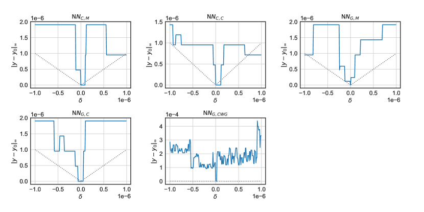
Figure 1: Change of logits vector due to small single-element input perturbations for different implementations. The dashed lines are $y=|\delta|$.

Observation 2: Different neural network implementations exhibit different floating point error characteristics. We evaluate the implementations on the whole MNIST test set and compare the outputs of the first layer (i.e., with only one linear transformation applied to the input) against that of $\operatorname{NN_{C,M}}$. Figure 2 presents the histogram which shows that different implementations usually manifest different error behavior.

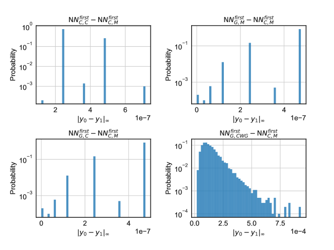
Figure 2: Distribution of difference relative to $\operatorname{NN_{C,M}}$ of first layer evaluated on MNIST test images.

Method Overview: Given a network and weights $\operatorname{NN}\left(\bm{\cdot};\,\bm{W}\right)$, we search for image pairs $(\bm{x_{0}},\bm{x_{1}})$ such that the network is verifiably robust with respect to $\bm{x_{0}}$, while $\bm{x_{1}}\in\operatorname{Adv}_{\epsilon}\left(\bm{\bm{x_{0}}}\right)$ and $L_{\operatorname{CW}}\left(\operatorname{NN}\left(\bm{x_{1}};\,\bm{W}\right),\,t_{0}\right)$ is less than the numerical fluctuation introduced by tiny input perturbations. We call $\bm{x_{0}}$ a quasi-safe image and $\bm{x_{1}}$ the corresponding quasi-adversarial image. Observation 1 suggests that an adversarial image might be obtained by randomly disturbing the quasi-adversarial image in the perturbation space. Observation 2 suggests that each implementation has its own adversarial images and needs to be handled separately. We search for the quasi-safe image by modifying the brightness of a natural image while querying a complete verifier whether it is near the boundary of robust predictions. Figure 3 illustrates this process.

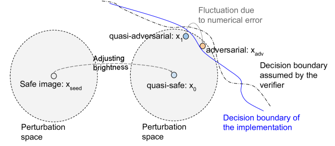
Figure 3: Illustration of our method. Since the verifier does not model the floating point arithmetic details of the implementation, their decision boundaries for the classification problem diverge, which allows us to find adversarial inputs that cross the boundary via numerical error fluctuations. Note that the verifier usually does not comply with a well defined specification of $\operatorname{NN}\left(\bm{\cdot};\,\bm{W}\right)$, and therefore it does not define a decision boundary. The dashed boundary in the diagram is just for illustrative purposes.

Before explaining the details of our method, we first present the following proposition that formally establishes the existence of quasi-safe and quasi-adversarial images for continuous neural networks:

Proposition 1

Let $E>0$ be an arbitrarily small positive number. If a continuous neural network $\operatorname{NN}\left(\bm{\cdot};\,\bm{W}\right)$ can produce a robust classification for some input belonging to class $t$, and it does not constantly classify all inputs as class $t$, then there exists an input $\bm{x_{0}}$ such that

$$0<\min_{\bm{x}\in\operatorname{Adv}_{\epsilon}\left(\bm{\bm{x_{0}}}\right)}L_{\operatorname{CW}}\left(\operatorname{NN}\left(\bm{x};\,\bm{W}\right),\,t\right)<E$$

Let $\bm{x_{1}}=\operatorname{argmin}_{\bm{x}\in\operatorname{Adv}_{\epsilon}\left(\bm{\bm{x_{0}}}\right)}L_{\operatorname{CW}}\left(\operatorname{NN}\left(\bm{x};\,\bm{W}\right),\,t\right)$ be the minimizer of the above function. We call $\bm{x_{0}}$ a quasi-safe image and $\bm{x_{1}}$ a quasi-adversarial image.

Proof

Let $f(\bm{x})\vcentcolon=\min_{\bm{x}^{\prime}\in\operatorname{Adv}_{\epsilon}\left(\bm{x}\right)}L_{\operatorname{CW}}\left(\operatorname{NN}\left(\bm{x^{\prime}};\,\bm{W}\right),\,t\right)$. Since $f(\cdot)$ is composed of continuous functions, $f(\cdot)$ is continuous. Suppose $\operatorname{NN}\left(\bm{\cdot};\,\bm{W}\right)$ is robust with respect to $\bm{x_{+}}$ that belongs to class $t$. Let $\bm{x_{-}}$ be be any input such that $L_{\operatorname{CW}}\left(\operatorname{NN}\left(\bm{x_{-}};\,\bm{W}\right),\,t\right)<0$, which exists because $\operatorname{NN}\left(\bm{\cdot};\,\bm{W}\right)$ does not constantly classify all inputs as class $t$. We have $f(\bm{x_{+}})>0$ and $f(\bm{x_{-}})<0$. The Poincaré-Miranda theorem asserts the existence of $\bm{x_{0}}$ such that $0<f(\bm{x_{0}})<E$.

Given a particular implementation $\operatorname{NN_{impl}}\left(\bm{\cdot};\,\bm{W}\right)$ and a natural image $\bm{x_{\operatorname{seed}}}$ which the network robustly classifies as class $t_{0}$ according to the verifier, we construct an adversarial input pair $(\bm{x_{0}},\,\bm{x_{\operatorname{adv}}})$ that meets the constraints described in Section 3 in three steps:

Step 1: We search for a coefficient $\alpha\in[0,1]$ such that $\bm{x_{0}}=\alpha\bm{x_{\operatorname{seed}}}$ serves as the quasi-safe image. Specifically, we require the verifier to claim that the network is robust for $\alpha\bm{x_{\operatorname{seed}}}$ but not so for $\alpha^{\prime}\bm{x_{\operatorname{seed}}}$ with $0<(\delta=\alpha-\alpha^{\prime})<\epsilon_{r}$, where $\epsilon_{r}$ should be small enough to allow quasi-adversarial images sufficiently close to the boundary. We set $\epsilon_{r}=10^{-7}$. We use binary search to minimize $\delta$ starting from $\alpha^{\prime}\leftarrow 0$, $\alpha\leftarrow 1$. We found that the MILP solver often becomes extremely slow when $\delta$ is small, so we start with binary search and switch to grid search by dividing the best known $\delta$ to 16 intervals if the solver exceeds a time limit.

Step 2: We search for the quasi-adversarial image $\bm{x_{1}}$ corresponding to $\bm{x_{0}}$. We define a loss function with a tolerance of $\tau$ as $L(\bm{x},\,\tau)\vcentcolon=L_{\operatorname{CW}}\left(\operatorname{NN}\left(\bm{x};\,\bm{W}\right),\,t_{0}\right)-\tau$, which can be incorporated in any verifier by modifying the bias of the Softmax layer. We aim to find $\tau_{0}$ and $\tau_{1}$, where $\tau_{0}$ is the minimal confidence of all images in the perturbation space of $\bm{x_{0}}$, and $\tau_{1}$ is slightly larger than $\tau_{0}$ with $\bm{x_{1}}$ being the corresponding adversarial image. Formally:

$$\left\{\begin{array}[]{l}\forall\bm{x}\in\operatorname{Adv}_{\epsilon}\left(\bm{x_{0}}\right):\>L(\bm{x},\,\tau_{0})>0\\ \bm{x_{1}}\in\operatorname{Adv}_{\epsilon}\left(\bm{x_{0}}\right)\\ L(\bm{x_{1}},\,\tau_{1})<0\\ \tau_{1}-\tau_{0}<10^{-7}\end{array}\right.$$

Note that $\bm{x_{1}}$ is produced by the complete verifier as proof of nonrobustness given the tolerance $\tau_{1}$. The above values are found via binary search with initialization $\tau_{0}\leftarrow 0$ and $\tau_{1}\leftarrow L_{\operatorname{CW}}\left(\operatorname{NN}\left(\bm{x_{0}};\,\bm{W}\right),\,t_{0}\right)$. In addition, we accelerate the binary search if the verifier can compute the worst objective defined as:

$$\tau_{w}=\min_{\bm{x}\in\operatorname{Adv}_{\epsilon}\left(\bm{x_{0}}\right)}L_{\operatorname{CW}}\left(\operatorname{NN}\left(\bm{x};\,\bm{W}\right),\,t_{0}\right)$$ (7)

In this case, we initialize $\tau_{0}\leftarrow\tau_{w}-\delta_{s}$ and $\tau_{1}\leftarrow\tau_{w}+\delta_{s}$. We empirically set $\delta_{s}=3\times 10^{-6}$ to incorporate the numerical error in the verifier so that $L(\bm{x_{0}},\,\tau_{w}-\delta_{s})>0$ and $L(\bm{x_{0}},\,\tau_{w}+\delta_{s})<0$. The binary search is aborted if the solver times out.

Step 3: We minimize $L_{\operatorname{CW}}\left(\operatorname{NN}\left(\bm{x_{1}};\,\bm{W}\right),\,t_{0}\right)$ with hill climbing via applying small random perturbations on the quasi-adversarial image $\bm{x_{1}}$ while projecting back to $\operatorname{Adv}_{\epsilon}\left(\bm{x_{0}}\right)$ to find an adversarial example. The perturbations are applied on patches of $\bm{x_{1}}$ as described in Algorithm 1.

Algorithm 1 Searching adversarial examples via hill climbing

Input: quasi-safe image $\bm{x_{0}}$

Input: target class number $t$

Input: quasi-adversarial image $\bm{x_{1}}$

Input: input perturbation bound $\epsilon$

Input: a neural network inference implementation $\operatorname{NN_{impl}}\left(\bm{\cdot};\,\bm{W}\right)$

Input: number of iterations $N$ (default value $1000$)

Input: perturbation scale $u$ (default value ${2}\mathrm{e}{-7}$)

Output: an adversarial image $\bm{x_{\operatorname{adv}}}$ or FAILED

for Index $i$ of $\bm{x_{0}}$ do $\triangleright$ Find the bounds $\bm{x_{l}}$ and $\bm{x_{u}}$ for allowed perturbations

    $x_{l}[i]\leftarrow\max(\operatorname{nextafter}(x_{0}[i]-\epsilon,\,0),\,0)$

    $x_{u}[i]\leftarrow\min(\operatorname{nextafter}(x_{0}[i]+\epsilon,\,1),\,1)$

    while ${x_{0}[i]-x_{l}[i]}>\epsilon$ or ${\operatorname{float64}\left(x_{0}[i]\right)-\operatorname{float64}\left(x_{l}[i]\right)}>\epsilon$ do

        $x_{l}[i]\leftarrow\operatorname{nextafter}(x_{l}[i],1)$

    end while

    while ${x_{u}[i]-x_{0}[i]}>\epsilon$ or ${\operatorname{float64}\left(x_{u}[i]\right)-\operatorname{float64}\left(x_{0}[i]\right)}>\epsilon$ do

        $x_{u}[i]\leftarrow\operatorname{nextafter}(x_{u}[i],0)$

    end while

end for $\triangleright$ We select the offset and stride based on the implementation to ensure that perturbed tiles contribute independently to the output. The Winograd algorithm in cuDNN produces $9\times 9$ output tiles for $13\times 13$ input tiles and $5\times 5$ kernels.

if $\operatorname{NN_{impl}}\left(\bm{\cdot};\,\bm{W}\right)$ is $\operatorname{NN_{G,CWG}}\left(\bm{\cdot};\,\bm{W}\right)$ then $(\operatorname{offset},\,\operatorname{stride})\leftarrow(4,9)$

else    $(\operatorname{offset},\,\operatorname{stride})\leftarrow(0,4)$

end if

for $i\leftarrow 1$ to $N$ do

    for $(h,w)\leftarrow(0,\,0)$ to $(\operatorname{height}(\bm{x_{1}}),\,\operatorname{width}(\bm{x_{1}}))$ step $(\operatorname{stride},\,\operatorname{stride})$  do

        $\delta\leftarrow\operatorname{uniform}(-u,\,u,\,(\operatorname{stride}-\operatorname{offset},\,\operatorname{stride}-\operatorname{offset}))$

        $\bm{x_{1}}^{\prime}\leftarrow\bm{x_{1}}[:]$

        $\bm{x_{1}}^{\prime}[h+\operatorname{offset}:h+\operatorname{stride},\,w+\operatorname{offset}:w+\operatorname{stride}]\mathrel{+}\mathrel{\mkern-1.0mu}=\delta$

        $\bm{x_{1}}^{\prime}\leftarrow\max(\min(\bm{x_{1}}^{\prime},\,\bm{x_{u}}),\,\bm{x_{l}})$

        if $L_{\operatorname{CW}}\left(\operatorname{NN_{impl}}\left(\bm{\bm{x_{1}}^{\prime}};\,\bm{W}\right),\,t\right)<L_{\operatorname{CW}}\left(\operatorname{NN_{impl}}\left(\bm{\bm{x_{1}}};\,\bm{W}\right),\,t\right)$ then

           $\bm{x_{1}}\leftarrow\bm{x_{1}}^{\prime}$

        end if

    end for

end for

if $L_{\operatorname{CW}}\left(\operatorname{NN_{impl}}\left(\bm{\bm{x_{1}}};\,\bm{W}\right),\,t\right)<0$ then return $\bm{x_{\operatorname{adv}}}\leftarrow\bm{x_{1}}$

else    return FAILED

end if

Experiments: We conduct our experiments on a workstation with an NVIDIA Titan RTX GPU and an AMD Ryzen Threadripper 2970WX CPU. We train the small architecture from Xiao et al. [48] with the PGD adversary and the RS Loss on MNIST and CIFAR10 datasets. The network has two convolutional layers with $4\times 4$ filters, $2\times 2$ stride, and 16 and 32 output channels, respectively, and two fully connected layers with 100 and 10 output neurons. The trained networks achieve 94.63% and 44.73% provable robustness with perturbations of $\ell_{\infty}$ bounded by $0.1$ and $2/255$ on the two datasets, respectively, similar to the results reported in Xiao et al. [48]. Our code is available at https://github.com/jia-kai/realadv.

Although our method only needs $O(-\log\epsilon)$ invocations of the verifier where $\epsilon$ is the threshold in the binary search, the verifier still takes most of the time and is too slow for a large benchmark. Therefore, for each dataset, we test our method on $32$ images randomly sampled from the verifiably robustly classified test images. All the implementations that we have considered are successfully exploited. Specifically, our benchmark contains $32\times 2\times 5=320$ cases, while adversarial examples are found for $82$ of them. The failed cases correspond to large $\tau_{1}$ values in Step 2 due to verifier timeouts or the discrepancy of floating point arithmetic between the verifier and the implementations. Let $\operatorname{\tau_{impl}}\vcentcolon=L_{\operatorname{CW}}\left(\operatorname{NN_{impl}}\left(\bm{\bm{x_{1}}};\,\bm{W}\right),\,t\right)$ denote the loss of an quasi-adversarial input on a particular implementation. Algorithm 1 succeeds on all cases with $\operatorname{\tau_{impl}}<8.3\times 10^{-7}$ ($35$ such cases in total), while $18$ among them have $\operatorname{\tau_{impl}}<0$ due to floating point discrepancy (i.e., the quasi-adversarial input is already an adversarial input for this implementation). The most challenging case (i.e., with largest $\operatorname{\tau_{impl}}$) on which Algorithm 1 succeeds has $\operatorname{\tau_{impl}}=3.2\times 10^{-4}$. The largest value of $\operatorname{\tau_{impl}}$ is $3.7$. Table 1 presents the detailed numbers for each implementation. Figure 4 shows the quasi-safe images on which our exploitation method succeeds for all implementations and the corresponding adversarial images.

Table 1: Number of adversarial examples successfully found for different neural network inference implementations

	$\operatorname{NN_{C,M}}$	$\operatorname{NN_{C,C}}$	$\operatorname{NN_{G,M}}$	$\operatorname{NN_{G,C}}$	$\operatorname{NN_{G,CWG}}$
MNIST	2	3	1	3	7
CIFAR10	16	12	7	6	25

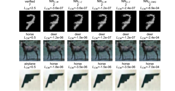
Figure 4: The quasi-safe images with respect to which all implementations are successfully exploited, and the corresponding adversarial images.

5 Exploiting an incomplete verifier

The relaxation adopted in certification methods renders them incomplete but also makes their verification claims more robust to floating point error compared to complete verifiers. In particular, we evaluate the CROWN framework [49] on our randomly selected MNIST test images and the corresponding quasi-safe images from Section 4. CROWN is able to verify the robustness of the network on $29$ out of the $32$ original test images, but it is unable to prove the robustness for any of the quasi-safe images. Note that MIPVerify claims that the network is robust with respect to all the original test images and the corresponding quasi-safe images.

Incomplete verifiers are still vulnerable if we allow arbitrary network architectures and weights. Our exploitation builds on the observation that verifiers typically need to merge always-active ReLU units with their subsequent layers to reduce the number of nonlinearities and achieve a reasonable speed. The merge of layers involves computing merged “equivalent” weights, which is different from the floating point computation adopted by an inference implementation.

We build a neural network that takes a $13\times 13$ single-channel input image, followed by a $5\times 5$ convolutional layer with a single output channel, two fully connected layers with $16$ output neurons each, a fully connected layer with one output neuron denoted as $u=\max(\bm{W_{u}}\bm{h_{u}}+b_{u},\,0)$, and a final linear layer that computes $\bm{y}=[u;\,10^{-7}]$ as the logits vector. All the hidden layers have ReLU activation. The input $\bm{x_{0}}$ is taken from a Gaussian distribution. The hidden layers have random Gaussian coefficients, and the biases are chosen so that (i) the ReLU neurons before $u$ are always activated for inputs in the perturbation space of $\bm{x_{0}}$ (ii) the neuron $u$ is never activated while $b_{u}$ is the maximum possible value (i.e., $b_{u}=-\max_{\bm{x}\in\operatorname{Adv}_{\epsilon}\left(\bm{x_{0}}\right)}\bm{W_{u}}\bm{h_{u}}(\bm{x})$) . CROWN is able to prove that all ReLU neurons before $u$ are always activated but $u$ is never activated, and therefore it claims that the network is robust with respect to perturbations around $\bm{x_{0}}$. However, by initializing the quasi-adversarial input $\bm{x_{1}}\leftarrow\bm{x_{0}}+\epsilon\operatorname{sign}(\bm{W_{equiv}})$ where $\bm{W_{equiv}}$ is the product of all the coefficient matrices of the layers up to $u$, we successfully find adversarial inputs for all the five implementations considered in this work by randomly perturbing $\bm{x_{1}}$ using Algorithm 1 with a larger number of iterations ($N=10000$) due to the smaller input size.

Note that the output scores can be manipulated to appear less suspicious. For instance, we can set $\bm{z}=\operatorname{clip}(10^{7}\cdot\bm{y},\,-2,\,2)$ as the final output in the above example so that $\bm{z}$ becomes a more “naturally looking” classification score in the range $[-2,\,2]$ and its perturbation due to floating point error is also enlarged to the unit scale. The extreme constants $10^{-7}$ and $10^{7}$ can also be obfuscated by using multiple consecutive scaling layers with each one having small scaling factors such as $0.1$ and $10$.

6 Discussion

We have shown that some neural network verifiers are systematically exploitable. One appealing remedy is to introduce relaxations into complete verifiers, such as by verifying for a larger $\epsilon$ or setting a threshold for accepted confidence score. For example, it might be tempting to claim the robustness of a network for $\epsilon=0.09999$ if it is verified for $\epsilon=0.1$. We emphasize that there are no guarantees provided by any floating point complete verifier currently extant. Moreover, the difference between the true robust perturbation bound and the bound claimed by an unsound verifier might be much larger if the network has certain properties. For example, MIPVerify has been observed to give NaN results when verifying pruned neural networks [15]. The adversary might also be able to manipulate the network to scale the scores arbitrarily, as discussed in Section 5. The correct solution requires obtaining a tight relaxation bound that is sound for both the verifier and the inference implementation, which is extremely challenging.

A possible fix for complete verification is to adopt exact MILP solvers with rational inputs [39]. There are three challenges: (i) The efficiency of exactly solving the large amounts of computation in neural network inference has not been studied and is unlikely to be satisfactory (ii) The computation that derives the MILP formulation from a verification specification, such as the neuron bound analysis in Tjeng et al. [42], must also be exact, but existing neural network verifiers have not attempted to define and implement exact arithmetic with the floating point weights (iii) The results of exact MILP solvers are only valid for an exact neural network inference implementation, but such exact implementations are not widely available (not provided by any deep learning libraries that we are aware of), and their efficiency remains to be studied .

Alternatively, one may obtain sound and nearly complete verification by adopting a conservative MILP solver based on techniques such as directed rounding [28]. We also need to ensure all arithmetic in the verifier to derive the MILP formulation soundly over-approximates floating point error. This is more computationally feasible than exact verification discussed above. It is similar to the approach used in some sound incomplete verifiers that incorporate floating point error by maintaining upper and lower rounding bounds of internal computations [36, 37]. However, this approach relies on the specific implementation details of the inference algorithm — optimizations such as Winograd [22] or FFT [1], or deployment in hardware accelerators with lower floating point precision such as Bfloat16 [4], would either invalidate the robustness guarantees or require changes to the analysis algorithm. Therefore, we suggest that these sound verifiers explicitly state the requirements on the inference implementations for which their results are sound. A possible future research direction is to devise a universal sound verification framework that can incorporate different inference implementations.

Another approach for sound and complete neural network verification is to quantize the computation to align the inference implementation with the verifier. For example, if we require all activations to be multiples of $s_{0}$ and all weights to be multiples of $s_{1}$, where $s_{0}s_{1}>2E$ and $E$ is a very loose bound of possible implementation error, then the output can be rounded to multiples of $s_{0}s_{1}$ to completely eliminate numerical error. Binarized neural networks [18] are a family of extremely quantized networks, and their verification [27, 35, 20] is sound and complete. However, the problem of robust training and verification of quantized neural networks [20] is relatively under-examined compared to that of real-valued neural networks [24, 26, 42, 48].

7 Conclusion

Floating point error should not be overlooked in the verification of real-valued neural networks, as we have presented techniques that efficiently find witnesses for the unsoundness of two verifiers. Unfortunately, floating point soundness issues have not received sufficient attention in neural network verification research. A user has few choices if they want to obtain sound verification results for a neural network, especially if they deploy accelerated neural network inference implementations. We hope our results will help to guide future neural network verification research by providing another perspective on the tradeoff between soundness, completeness, and scalability.

Acknowledgments

We would like to thank Gagandeep Singh and Kai Xiao for providing invaluable suggestions on an early manuscript.

References

- Abtahi et al. [2018] Abtahi, T., Shea, C., Kulkarni, A., Mohsenin, T.: Accelerating convolutional neural network with FFT on embedded hardware. IEEE Transactions on Very Large Scale Integration (VLSI) Systems 26(9), 1737–1749 (2018)
- Boldo and Melquiond [2017] Boldo, S., Melquiond, G.: Computer Arithmetic and Formal Proofs: Verifying Floating-point Algorithms with the Coq System. Elsevier (2017)
- Bunel et al. [2020] Bunel, R., Lu, J., Turkaslan, I., Kohli, P., Torr, P., Mudigonda, P.: Branch and bound for piecewise linear neural network verification. Journal of Machine Learning Research 21(2020) (2020)
- Burgess et al. [2019] Burgess, N., Milanovic, J., Stephens, N., Monachopoulos, K., Mansell, D.: Bfloat16 processing for neural networks. In: 2019 IEEE 26th Symposium on Computer Arithmetic (ARITH), pp. 88–91, IEEE (2019)
- Carlini and Wagner [2017] Carlini, N., Wagner, D.: Towards evaluating the robustness of neural networks. In: 2017 ieee symposium on security and privacy (sp), pp. 39–57, IEEE (2017)
- Cheng et al. [2017] Cheng, C.H., Nührenberg, G., Ruess, H.: Maximum resilience of artificial neural networks. In: International Symposium on Automated Technology for Verification and Analysis, pp. 251–268, Springer (2017)
- Chetlur et al. [2014] Chetlur, S., Woolley, C., Vandermersch, P., Cohen, J., Tran, J., Catanzaro, B., Shelhamer, E.: cudnn: Efficient primitives for deep learning. arXiv preprint arXiv:1410.0759 (2014)
- Corzilius et al. [2012] Corzilius, F., Loup, U., Junges, S., Ábrahám, E.: Smt-rat: an smt-compliant nonlinear real arithmetic toolbox. In: International Conference on Theory and Applications of Satisfiability Testing, pp. 442–448, Springer (2012)
- Das et al. [2020] Das, A., Briggs, I., Gopalakrishnan, G., Krishnamoorthy, S., Panchekha, P.: Scalable yet rigorous floating-point error analysis. In: SC20, pp. 1–14, IEEE (2020)
- Dutta et al. [2018] Dutta, S., Jha, S., Sankaranarayanan, S., Tiwari, A.: Output range analysis for deep feedforward neural networks. In: NASA Formal Methods Symposium, pp. 121–138, Springer (2018)
- Dvijotham et al. [2018] Dvijotham, K., Gowal, S., Stanforth, R., Arandjelovic, R., O’Donoghue, B., Uesato, J., Kohli, P.: Training verified learners with learned verifiers. arXiv preprint arXiv:1805.10265 (2018)
- Ehlers [2017] Ehlers, R.: Formal verification of piece-wise linear feed-forward neural networks. In: International Symposium on Automated Technology for Verification and Analysis, pp. 269–286, Springer (2017)
- Fischetti and Jo [2018] Fischetti, M., Jo, J.: Deep neural networks and mixed integer linear optimization. Constraints 23(3), 296–309 (2018)
- Gehr et al. [2018] Gehr, T., Mirman, M., Drachsler-Cohen, D., Tsankov, P., Chaudhuri, S., Vechev, M.: Ai2: Safety and robustness certification of neural networks with abstract interpretation. In: 2018 IEEE Symposium on Security and Privacy (SP), pp. 3–18, IEEE (2018)
- Guidotti et al. [2020] Guidotti, D., Leofante, F., Pulina, L., Tacchella, A.: Verification of neural networks: Enhancing scalability through pruning. arXiv preprint arXiv:2003.07636 (2020)
- Gurobi Optimization [2020] Gurobi Optimization, L.: Gurobi optimizer reference manual (2020), URL http://www.gurobi.com
- Huang et al. [2017] Huang, X., Kwiatkowska, M., Wang, S., Wu, M.: Safety verification of deep neural networks. In: International Conference on Computer Aided Verification, pp. 3–29, Springer (2017)
- Hubara et al. [2016] Hubara, I., Courbariaux, M., Soudry, D., El-Yaniv, R., Bengio, Y.: Binarized neural networks. In: NeurIPS, pp. 4107–4115, Curran Associates, Inc. (2016)
- IEEE [2008] IEEE: IEEE standard for floating-point arithmetic. IEEE Std 754-2008 pp. 1–70 (2008)
- Jia and Rinard [2020] Jia, K., Rinard, M.: Efficient exact verification of binarized neural networks. In: NeurIPS, vol. 33, pp. 1782–1795, Curran Associates, Inc. (2020)
- Katz et al. [2017] Katz, G., Barrett, C., Dill, D.L., Julian, K., Kochenderfer, M.J.: Reluplex: An efficient smt solver for verifying deep neural networks. In: International Conference on Computer Aided Verification, pp. 97–117, Springer (2017)
- Lavin and Gray [2016] Lavin, A., Gray, S.: Fast algorithms for convolutional neural networks. In: Proceedings of the IEEE Conference on Computer Vision and Pattern Recognition, pp. 4013–4021 (2016)
- Lomuscio and Maganti [2017] Lomuscio, A., Maganti, L.: An approach to reachability analysis for feed-forward relu neural networks. arXiv preprint arXiv:1706.07351 (2017)
- Madry et al. [2018] Madry, A., Makelov, A., Schmidt, L., Tsipras, D., Vladu, A.: Towards deep learning models resistant to adversarial attacks. In: ICLR (2018)
- Miné [2004] Miné, A.: Relational abstract domains for the detection of floating-point run-time errors. In: European Symposium on Programming, pp. 3–17, Springer (2004)
- Mirman et al. [2018] Mirman, M., Gehr, T., Vechev, M.: Differentiable abstract interpretation for provably robust neural networks. In: Dy, J., Krause, A. (eds.) Proceedings of the 35th International Conference on Machine Learning, Proceedings of Machine Learning Research, vol. 80, pp. 3578–3586, PMLR, Stockholmsmässan, Stockholm Sweden (10–15 Jul 2018)
- Narodytska et al. [2018] Narodytska, N., Kasiviswanathan, S., Ryzhyk, L., Sagiv, M., Walsh, T.: Verifying properties of binarized deep neural networks. In: Thirty-Second AAAI Conference on Artificial Intelligence (2018)
- Neumaier and Shcherbina [2004] Neumaier, A., Shcherbina, O.: Safe bounds in linear and mixed-integer linear programming. Mathematical Programming 99(2), 283–296 (2004)
- Paszke et al. [2019] Paszke, A., Gross, S., Massa, F., Lerer, A., Bradbury, J., Chanan, G., Killeen, T., Lin, Z., Gimelshein, N., Antiga, L., Desmaison, A., Kopf, A., Yang, E., DeVito, Z., Raison, M., Tejani, A., Chilamkurthy, S., Steiner, B., Fang, L., Bai, J., Chintala, S.: PyTorch: An imperative style, high-performance deep learning library. In: NeurIPS, pp. 8024–8035, Curran Associates, Inc. (2019)
- Raghu and Schmidt [2020] Raghu, M., Schmidt, E.: A survey of deep learning for scientific discovery. ArXiv abs/2003.11755 (2020)
- Raghunathan et al. [2018] Raghunathan, A., Steinhardt, J., Liang, P.S.: Semidefinite relaxations for certifying robustness to adversarial examples. In: NeurIPS, pp. 10877–10887, Curran Associates, Inc. (2018)
- Rümmer and Wahl [2010] Rümmer, P., Wahl, T.: An smt-lib theory of binary floating-point arithmetic. In: International Workshop on Satisfiability Modulo Theories (SMT), p. 151 (2010)
- Salman et al. [2019] Salman, H., Yang, G., Zhang, H., Hsieh, C.J., Zhang, P.: A convex relaxation barrier to tight robustness verification of neural networks. In: NeurIPS, pp. 9832–9842 (2019)
- Scheibler et al. [2015] Scheibler, K., Winterer, L., Wimmer, R., Becker, B.: Towards verification of artificial neural networks. In: MBMV, pp. 30–40 (2015)
- Shih et al. [2019] Shih, A., Darwiche, A., Choi, A.: Verifying binarized neural networks by angluin-style learning. In: International Conference on Theory and Applications of Satisfiability Testing, pp. 354–370, Springer (2019)
- Singh et al. [2018] Singh, G., Gehr, T., Mirman, M., Püschel, M., Vechev, M.: Fast and effective robustness certification. In: NeurIPS, pp. 10802–10813, Curran Associates, Inc. (2018)
- Singh et al. [2019] Singh, G., Gehr, T., Püschel, M., Vechev, M.T.: An abstract domain for certifying neural networks. Proceedings of the ACM on Programming Languages 3, 1 – 30 (2019)
- Solovyev et al. [2018] Solovyev, A., Baranowski, M.S., Briggs, I., Jacobsen, C., Rakamarić, Z., Gopalakrishnan, G.: Rigorous estimation of floating-point round-off errors with symbolic taylor expansions. TOPLAS 41(1), 1–39 (2018)
- Steffy and Wolter [2013] Steffy, D.E., Wolter, K.: Valid linear programming bounds for exact mixed-integer programming. INFORMS Journal on Computing 25(2), 271–284 (2013)
- Szegedy et al. [2014] Szegedy, C., Zaremba, W., Sutskever, I., Estrach, J.B., Erhan, D., Goodfellow, I., Fergus, R.: Intriguing properties of neural networks. In: ICLR (2014)
- Titolo et al. [2018] Titolo, L., Feliú, M.A., Moscato, M.M., Muñoz, C.A.: An abstract interpretation framework for the round-off error analysis of floating-point programs. In: VMCAI, pp. 516–537 (2018)
- Tjeng et al. [2019] Tjeng, V., Xiao, K.Y., Tedrake, R.: Evaluating robustness of neural networks with mixed integer programming. In: ICLR (2019)
- Tramer and Boneh [2019] Tramer, F., Boneh, D.: Adversarial training and robustness for multiple perturbations. In: NeurIPS, pp. 5866–5876, Curran Associates, Inc. (2019)
- Wang et al. [2018] Wang, S., Pei, K., Whitehouse, J., Yang, J., Jana, S.: Formal security analysis of neural networks using symbolic intervals. In: 27th USENIX Security Symposium (USENIX Security 18), pp. 1599–1614 (2018)
- Weng et al. [2018] Weng, L., Zhang, H., Chen, H., Song, Z., Hsieh, C.J., Daniel, L., Boning, D., Dhillon, I.: Towards fast computation of certified robustness for ReLU networks. In: International Conference on Machine Learning, pp. 5276–5285 (2018)
- Wong and Kolter [2017] Wong, E., Kolter, J.Z.: Provable defenses against adversarial examples via the convex outer adversarial polytope. arXiv preprint arXiv:1711.00851 (2017)
- Wong et al. [2020] Wong, E., Rice, L., Kolter, J.Z.: Fast is better than free: Revisiting adversarial training. In: ICLR (2020)
- Xiao et al. [2019] Xiao, K.Y., Tjeng, V., Shafiullah, N.M.M., Madry, A.: Training for faster adversarial robustness verification via inducing reLU stability. In: ICLR (2019)
- Zhang et al. [2018] Zhang, H., Weng, T.W., Chen, P.Y., Hsieh, C.J., Daniel, L.: Efficient neural network robustness certification with general activation functions. In: NeurIPS, pp. 4939–4948, Curran Associates, Inc. (2018)