Protecting Quantum Fisher Information in Correlated Quantum Channels

Abstract

Quantum Fisher information (QFI) has potential applications in quantum metrology tasks. We investigate QFI when the consecutive actions of a quantum channel on the sequence of qubits have partial classical correlations. Our results showed that while the decoherence effect is detrimental to QFI, effects of such classical correlations on QFI are channel-dependent. For the Bell-type probe states, the classical correlations on consecutive actions of the depolarizing and phase flip channels can be harnessed to improve QFI, while the classical correlations in the bit flip and bit-phase flip channels induce a slight decrease of QFI. For a more general parameterization form of the probe states, the advantage of using initial correlated system on improving QFI can also be remained in a wide regime of the correlated quantum channels.

I Introduction

In quantum estimation theory, one of the fundamental tasks is to estimate the values of the unobservable parameters in the labeled quantum system based on the set of measurement data metro1 ; metro2 ; metro3 . To improve the precision of such an estimation and to approach asymptotically the quantum limit of the estimation accuracy remain the main pursuits of this task. In this context, many relevant works have been done in the past years, among which the quantum Fisher information (QFI) was shown to be an essential quantity as the Cramér-Rao theorem shows that its inverse places a fundamental limit on the variance of the estimator Rao1 ; Rao2 . Due to this practical application, QFI has been studied from different aspects, with much notable progresses being achieved. For example, it has been adopted to derive a statistical generalization of the Heisenberg uncertainty relation Luosl . Its measurement with finite precision was demonstrated in deqfi , while its interconnections with quantum correlations qfi-qc1 ; qfi-qc2 ; qfi-qc3 ; qfi-qc4 and quantum coherence qfi-co1 ; qfi-co2 ; qfi-co3 have also been identified. Moreover, there are several other works focused on studying properties of QFI in certain explicit physical systems spin ; Dicke ; atom and the noninertial frames reff1 ; reff2 .

When implementing the parameter estimation tasks in laboratory, the quantum system for which the probe state is encoded in will unavoidably interacts with its surrounding environments. This may induce rapid decay of the quantum coherence of the state deco as well as its quantum correlations if the state is of bipartite or multipartite QE ; QD ; robu ; Hu ; Hulian . Of course, such an unwanted interaction is also detrimental to QFI in most cases deco1 ; deco2 ; deco3 ; deco4 ; deco5 ; prot1 ; prot2 , and remains a bottleneck restricting our ability to approach the quantum limit of the estimation accuracy. So it is of practical significance to seek efficient ways for protecting QFI of a system in noisy environments PhysRep .

Theoretically, one can regard all the unwanted effect caused by the inevitable interaction between the principle system and its surrounding environments as the sources of noises. In most cases, such a noisy effect can be characterized by a quantum channel transforming the input state into the output one. During this transformation process, the channel may retain partial memory about the history of its action on the sequence of qubits passing through it Nielsen . In general, there are two origins of the memory effects, i.e., the one occurs during the time evolution of each qubit due to the temporal correlations, and the one occurs between consecutive actions of the channel cc0 . The former memory effect may induce damped oscillations of quantum correlations such as entanglement and quantum discord QE ; QD ; robu ; Hu ; Hulian , while positive role of the latter memory effect on enhancing quantum coherence of two-qubit states Zhouw and reducing the entropic uncertainty of two incompatible observables eur have also been observed.

In this paper, we examine how the memory effect caused by the classical correlations between the consecutive actions of a channel affects QFI. We will show that while the decoherence effect induces rapid decay of the QFI, such a memory effect can be harnessed to delay evidently this decay. This result reveals distinct effects of the correlated and independent actions of a channel on the sequence of qubits on one hand, and on the other hand, is useful for improving the precision of parameter estimation of an open system. The structure of this paper is as follows. In Sec. II we recall briefly some preliminaries related to QFI and correlated quantum channels. Then in Sec. III, we investigate in detail influence of the correlated depolarizing, bit flip, bit-phase flip, and phase flip channels on QFI. Finally, Sec. IV is a conclusion remark of this work.

II Preliminaries

To begin with, we first recall briefly the notion of QFI and its calculation based on the spectral decomposition of the density operator. To define the QFI, we consider a probe state described by $\rho_{\theta}$ for which $\theta$ is an unobservable parameter, then the QFI with respect to $\theta$ can be written as metro2

$$F_{\theta}=\mathrm{Tr}(L_{\theta}^{2}\rho_{\theta}),$$ (1)

where $L_{\theta}$ is the symmetric logarithmic derivative determined by $\partial_{\theta}\rho_{\theta}=(L_{\theta}\rho_{\theta}+\rho_{\theta}L_{\theta})/2$.

By decomposing the density operator as $\rho_{\theta}=\sum_{i}\lambda_{i}|\psi_{i}\rangle\langle\psi_{i}|$, with $\lambda_{i}$ being the eigenvalues of $\rho_{\theta}$ and $|\psi_{i}\rangle$ the corresponding eigenstates, an analytical solution of QFI was derived as QFI ; Liuj

$$F_{\theta}=\sum_{i}\frac{(\lambda^{\prime}_{i})}{\lambda_{i}}^{2}+\sum_{i}{\lambda_{i}}{F_{\theta,i}}-\sum_{i\neq j}\frac{8\lambda_{i}\lambda_{j}}{\lambda_{i}+\lambda_{j}}|\langle\psi^{\prime}_{i}|\psi_{j}\rangle|^{2},$$ (2)

where we have denoted by

$$\lambda^{\prime}_{i}=\partial_{\theta}\lambda_{i},~{}|\psi^{\prime}_{i}\rangle=\partial_{\theta}|\psi_{i}\rangle,~{}F_{\theta,i}=4(\langle\psi^{\prime}_{i}|\psi^{\prime}_{i}\rangle-|\langle\psi^{\prime}_{i}|\psi_{i}\rangle|^{2}).$$ (3)

Obviously, $F_{\theta}$ is only determined by the support set of $\rho_{\theta}$ and is not affected by the eigenstates outside this support set. The first term in Eq. (2) is determined only by the eigenvalues of $\rho_{\theta}$ and is the classical contribution, while the second and third terms can be regarded as the quantum contribution.

An application of QFI is to describe the precision of parameter estimation metro1 ; metro2 ; metro3 . For instance, the quantum Cramér-Rao theorem cramer-rao shows that the minimum allowed variance of the unbiased estimator $\tilde{\theta}$ for $\theta$ is bounded by

$$\mathrm{Var}(\tilde{\theta})\geqslant\frac{1}{MF_{\theta}},$$ (4)

where $\mathrm{Var}(\tilde{\theta})=\langle\tilde{\theta}^{2}\rangle_{\rho_{\theta}}-\langle\tilde{\theta}\rangle^{2}_{\rho_{\theta}}$ , and $M\gg 1$ represents the times of repeated measurements.

Next, we introduce the correlated channel model. By taking $\rho_{0}$ as the input of the channel $\mathcal{E}$, then the output state after the system traversing the channel can be written as $\rho=\mathcal{E}(\rho_{0})$. In the operator-sum representation, we have $\mathcal{E}(\rho_{0})=\sum_{n}K_{n}\rho_{0}K_{n}^{\dagger}$, with $\{K_{n}\}$ being the Kraus operators describing actions of $\mathcal{E}$ on $\rho_{0}$ and they satisfy the completely positive and trace preserving relation $\sum_{n}K_{n}^{\dagger}K_{n}=\openone$ Nielsen . We focus on the Pauli channel and the $N$-qubit $\rho_{0}$, then the output state simplifies to

$$\rho=\sum_{i_{1}\cdots i_{N}}p_{i_{1}\cdots i_{N}}(\sigma_{i_{1}}\otimes\cdots\otimes\sigma_{i_{N}})\rho_{0}(\sigma_{i_{1}}\otimes\cdots\otimes\sigma_{i_{N}}),,$$ (5)

where $\sigma_{0}=\openone_{2}$ is the identity operator and $\sigma_{1,2,3}$ are the Pauli operators. If $\mathcal{E}$ acts independently and identically on each of the qubits traversing it, the joint probability will be given by $p_{i_{1}\cdots i_{N}}=p_{i_{1}}\cdots p_{i_{N}}$, with $p_{i}\geqslant 0$ and $\sum_{i}p_{i}=1$. Such a model describes the situation for which $\mathcal{E}$ has no memory on the history of its actions on the sequence of qubits.

In practice, the independent actions of the channel on those qubits traversing it is only a limiting case. When two or more qubits traverse the channel subsequently with short time interval, the channel may retain partial memory about its action on these qubits cc1 ; cc2 ; cc3 . Macchiavello and Palma cc1 proposed to describe such kind of memory effect by the classical correlations between consecutive uses of the channel, with the joint probability distribution function being given by

$$p_{i_{1}\cdots i_{N}}=p_{i_{1}}p_{i_{2}|i_{1}}\cdots p_{i_{N}|i_{N-1}},$$ (6)

where $p_{i_{n}|i_{n-1}}=(1-\mu)p_{i_{n}}+\mu\delta_{i_{n}i_{n-1}}$, with $\delta_{ij}=1$ for $i=j$ and $\delta_{ij}=0$ for $i\neq j$. Moreover, the parameter $\mu$ characterizes strength of the classical correlations. $\mu=0$ and 1 correspond respectively to the uncorrelated and fully correlated channels, while the intermediate value $0<\mu<1$ corresponds to a general classically correlated channel.

The completely positivity and trace preserving of the channel requires $\sum_{i}p_{i}=1$. There are many quantum channels satisfying this requirement Nielsen . We will focus on some paradigmatic instances of them. They are the depolarizing, bit flip, bit-phase flip, and phase flip channels which can be described by a parameter $p\in[0,1]$. For the depolarizing channel, the probability distribution function is given by

$$p_{0}^{\alpha_{0}}=1-p,~{}p_{1,2,3}^{\alpha_{0}}=\frac{p}{3},$$ (7)

and for the bit flip ($\alpha_{1}$), bit-phase flip ($\alpha_{2}$), and phase flip ($\alpha_{3}$) channels, they are given by

$$p_{0}^{\alpha_{k}}=1-p,~{}p_{k}^{\alpha_{k}}=p,~{}p_{i,j\neq k}^{\alpha_{k}}=0.$$ (8)

By combining these expressions with Eqs. (5) and (6), one can obtain the output state for any input state.

III QFI in correlated quantum channels

We now begin our discussion about how the classical correlations between consecutive uses of the channel affecting QFI. We take the following two-qubit state

$$|\Phi^{+}\rangle=\cos\theta|00\rangle+e^{i\varphi}\sin\theta|11\rangle,$$ (9)

as the input of the correlated quantum channels, where $\theta$ and $\varphi$ are unobservable parameters to be estimated. We will show explicitly that the QFI depends strongly on the type of quantum channels as well as strengths of the decoherence parameter and the classical correlations.

III.1 The correlated depolarizing channel

We first consider the case of correlated depolarizing channel. For the input state $|\Phi^{+}\rangle$, the nonzero elements of the density operator for the output state can be obtained as

$$\rho_{11}=A\cos^{2}{\theta}+C\sin^{2}{\theta},~{}\rho_{44}=1-\rho_{11}-2B,$$ (10)

$$\rho_{22,33}=B,~{}\rho_{14}=\rho_{41}^{*}=(De^{-i\varphi}+Ee^{i\varphi})\sin\theta\cos\theta,$$

where the corresponding parameters are given by

$$A=(1-\eta)(1-\eta+\eta\mu),$$ (11)

$$B=\eta(1-\eta)(1-\mu),~{}C=\eta^{2}+\eta(1-\eta)\mu,$$

$$D=(1-2\eta)^{2}+(3-4\eta)\eta\mu,~{}E=\eta\mu,$$

and here we have denoted by $\eta=2p/3$.

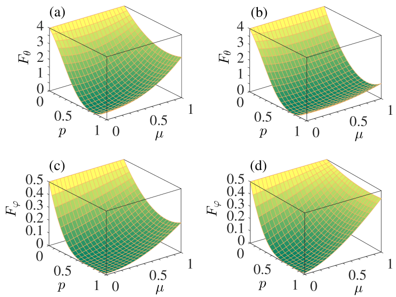
Figure 1: The $(p,\mu)$ dependence of $F_{\theta}$ and $F_{\varphi}$ for the input state $|\Phi^{+}\rangle$ and the correlated depolarizing channel. The parameters are $(\theta,\varphi)=(\pi/8,\pi/6)$ [(a) & (c)] and $(\pi/8,\pi/3)$ [(b) & (d)].

For this output state $\rho$, one can derive analytically its eigenvalues $\{\lambda_{i}\}$, its eigenvectors $\{|\psi_{i}\rangle\}$, and their partial derivatives with respect to both $\theta$ and $\varphi$ (see Appendix A). Then one can obtain directly the QFI by substituting these formulae into Eq. (2). We do not list their expressions here due to their complexity. Instead, we performed numerical calculation and showed in Fig. 1 the $(p,\mu)$ dependence of $F_{\theta}$ and $F_{\varphi}$.

It can be seen from the plots in Fig. 1 that with the increasing strength of the decoherence parameter $p$, both $F_{\theta}$ and $F_{\varphi}$ first decrease from their maxima to certain minimum values when $p$ reaches the critical point $0.75$, and then turn to be increased to some finite values smaller than those at $p=0$. This shows that the decoherence effect of the depolarizing channel is detrimental to QFI, and as a result, may reduce its usefulness for potential quantum tasks including parameter estimation. However, when considering the $\mu$ dependence of the QFI, one can note from Fig. 1(a) and (b) that in the regions of relative small $p$, $F_{\theta}$ first decreases to certain minimum values and then turn to be increased with the increasing strength of $\mu$ and reaches certain maximum values larger than those at $\mu=0$, while in the regions of large $p$, it increases monotonically in the whole region of $\mu$. Different from $F_{\theta}$, one can see from Fig. 1(c) and (d) that $F_{\varphi}$ is always a monotonic increasing function of $\mu$ for any $p>0$. Hence, effects of the classical correlation between consecutive actions of the channel on QFI is determined by both the strength of the decoherence parameter and the parameter to be estimated.

The above results show that the QFI can be noticeably enhanced in a wide region of the decoherence parameter due to the correlated actions of the depolarizing channel. This will be useful for its practical applications including parameter estimation in noisy environments. This is because the large value of QFI corresponds to a small value of the variance of the estimator, hence gives an improved estimation precision of the unobservable parameters cramer-rao .

III.2 The correlated bit flip and bit-phase flip channels

Next, we consider the case of two qubits traversing the classically correlated bit flip channel. The nonzero elements of the density operator for the output state can be obtained as

$$\rho_{11}=x\cos^{2}{\theta}+z\sin^{2}{\theta},~{}\rho_{22,33}=y,$$ (12)

$$\rho_{44}=1-\rho_{11}-2y,~{}\rho_{23,32}=y\sin 2\theta\cos\varphi,$$

$$\rho_{14}=\rho_{41}^{*}=(xe^{-i\varphi}+ze^{i\varphi})\sin\theta\cos\theta,$$

where $x$, $y$, and $z$ can be obtained respectively from $A$, $B$, and $C$ in Eq. (11) by substituting the parameter $\eta=2p/3$ with $\eta=p$. For this output state, though its explicit form is a little more complicated than that of Eq. (10), one can still derive analytical solutions of its eigenvalues $\{\lambda_{i}\}$, its eigenvectors $\{|\psi_{i}\rangle\}$, and the corresponding partial derivatives of them with respect to both $\theta$ and $\varphi$ (see Appendix B). Hence one can also derive straightforwardly analytical expressions of $F_{\theta}$ and $F_{\varphi}$.

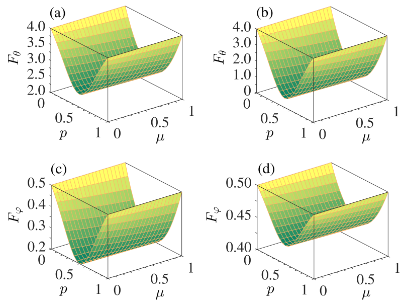
Figure 2: The $(p,\mu)$ dependence of $F_{\theta}$ and $F_{\varphi}$ for the input state $|\Phi^{+}\rangle$ and the correlated bit flip channel. The parameters are $(\theta,\varphi)=(\pi/8,\pi/6)$ [(a) & (c)] and $(\pi/8,\pi/3)$ [(b) & (d)].

By choosing the same parameters as those in Fig. 1, we performed numerical calculation and showed in Fig. 2 the exemplified plots of the $(p,\mu)$ dependence of $F_{\theta}$ and $F_{\varphi}$. From these plots one can see that they are symmetric with respect to $p=0.5$. In the region of $p\leqslant 0.5$, they decrease monotonically with the increase of $p$. This phenomenon is similar to the QFI for the depolarizing channel, and is also understandable as the parameters in Eq. (12) can be obtained by replacing $\eta=2p/3$ in Eq. (11) with $\eta=p$. However, due to the two extra nonzero elements $\rho_{23,32}$, the resulting $\mu$ dependence of $F_{\theta}$ and $F_{\varphi}$ are very different from those for the depolarizing channel. As was shown in Fig. 2, both $F_{\theta}$ and $F_{\varphi}$ were slightly decreased by the classical correlations between consecutive actions of the bit flip channel. But as their dependence on $\mu$ is weak, such a detrimental effect is also very weak.

For the same two qubits traversing the bit-phase flip channel, the density operator of the output state has a similar form to that for the bit flip channel. The only difference is that the matrix elements $\rho_{23,32}$ are multiplied by a minus. One can then show that the resulting $F_{\theta}$ and $F_{\varphi}$ have completely the same form to those for the bit flip channel.

III.3 The correlated phase flip channel

Now, we consider the case of two qubits traversing the correlated phase flip channel, for which the nonzero elements of the density operator for the output state are given by

$$\rho_{11}=\cos^{2}\theta,~{}\rho_{44}=\sin^{2}\theta,$$ (13)

$$\rho_{14}=\rho_{41}^{*}=we^{-i\varphi}\sin\theta\cos\theta,$$

where $w=1-4p(1-p)(1-\mu)$.

For this case, one can also derive analytically its eigenvalues $\{\lambda_{i}\}$, its eigenvectors $\{|\psi_{i}\rangle\}$, as well as their partial derivatives and the resulting QFI. In fact, by combing Eqs. (10) and (13), one can see that the corresponding QFI can be obtained directly by making the substitutions $A\rightarrow 1$, $(B,C,E)\rightarrow 0$, and $D\rightarrow w$ to those results showed in Appendix A.

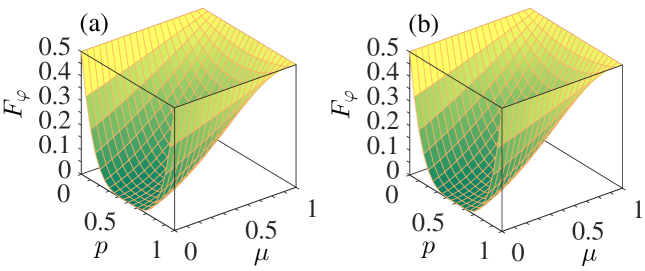
Figure 3: The $(p,\mu)$ dependence of $F_{\varphi}$ for the input state $|\Phi^{+}\rangle$ and the correlated phase flip channel. The parameters are $(\theta,\varphi)=(\pi/8,\pi/6)$ (a) and $(\pi/8,\pi/3)$ (b).

Our calculation shows that no matter what the strengths of $p$ and $\mu$ are, we always have $F_{\theta}=4$, i.e., it is immune of the phase flip channel. So we showed in Fig. 3 only the $(p,\mu)$ dependence of $F_{\varphi}$, which is symmetric with respect to $p=0.5$. This is in fact an immediate consequence of the form of $w$ below Eq. (13). In the region of $p\leqslant 0.5$, $F_{\varphi}$ decreases monotonically with the increasing strength of $p$, while for any fixed $p\neq\{0,1\}$, $F_{\varphi}$ behaves as a monotonic increasing function of $\mu$ and reaches its maximum value $F_{\varphi}^{\max}=\sin^{2}{2\theta}$ when $\mu=1$. This implies that the correlations between consecutive actions of the phase flip channel are always beneficial for improving QFI of the two-qubit state.

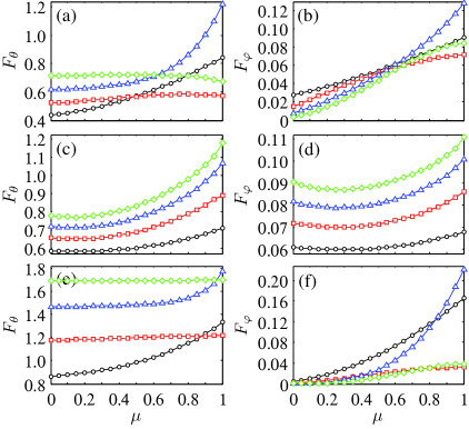
Figure 4: The $\mu$ dependence of $F_{\theta}$ and $F_{\varphi}$ for the input state $\rho_{0}^{EWL}$ with $p=0.3$, $(\theta,\varphi)=(\pi/8,\pi/6)$, $N=2$ (black circles), 3 (red squares), 4 (blue triangles), and 5 (green diamonds). The top two, middle two, and bottom two panels are plotted for the correlated depolarizing, bit flip, and phase flip channels, respectively.

We have also performed calculations for other Bell-type probe states including

$$|\Phi^{-}\rangle=\cos\theta|00\rangle-e^{i\varphi}\sin\theta|11\rangle,$$ (14)

$$|\Psi^{\pm}\rangle=\cos{\theta}|01\rangle\pm e^{i\varphi}\sin{\theta}|10\rangle,$$

and found that $F_{\theta}$ and $F_{\varphi}$ show qualitatively the same parameter dependence to those for the input state $|\Phi^{+}\rangle$. This confirms again our observation that the existence of classical correlations between consecutive actions of the quantum channel on a sequence of qubits are beneficial for improving the QFI. One may wonder whether the advantage of the correlated quantum channels on improving QFI can be remained for more general parameterization form of the probe states and for the probe states with different number of qubit. To give an answer to this concern, we further consider the following extended Werner-like probe state

$$\rho_{0}^{EWL}=r|\Xi\rangle\langle\Xi|+\frac{1-r}{2^{N}}\openone_{2^{N}},$$ (15)

where $|\Xi\rangle=\cos\theta|0\rangle^{\otimes N}+e^{i\varphi}\sin\theta|1\rangle^{\otimes N}$, and $r$ represents the ratio of the component $|\Xi\rangle$ in $\rho_{0}^{EWL}$. In Fig. 4, we presented an exemplified plot of the $\mu$ dependence of $F_{\theta}$ and $F_{\varphi}$ for $\rho_{0}^{EWL}$ with different qubit number $N$. It is clearly seen that the classical correlations between consecutive actions of the quantum channel give an improved QFI in a wide regime, hence the estimation precision of $\theta$ and $\varphi$ can also be improved evidently. For certain cases, the probe states with large number of qubit leads to a further improvement of the QFI compared with that with small number of qubit. This shows that the improved QFI due to correlated actions of a quantum channel may applies to very general input probe states.

Finally, we present an interpretation on the different behaviors of QFI for different quantum channels. Physically, such a difference is due to the interplay between correlations arising from the consecutive actions of the quantum channels on a sequence of qubits and the temporal correlations occurring in the evolution of each qubit. In particular, the temporal correlations are different for different quantum channels. Moreover, the correlated actions of a quantum channel leads to an inflow of information to the system cc1 ; cc2 ; cc3 , and this explains the improved QFI. As QFI is related to the variance of the quantum metrology, this further gives an improved estimation precision of the physical parameters.

IV Summary

In summary, we have explored effects of the classical correlations between consecutive actions of the quantum channel on QFI. Here, the classical correlations were characterized by the probability that the same Pauli transformation is applied to the sequence of qubits. We have considered the depolarizing, bit flip, bit-phase flip, and phase flip channels. For Bell-type probe states, it was found that the decoherence effect is always detrimental to QFI. On the other hand, effects of the classical correlations on QFI are different for different quantum channels: (i) For the correlated depolarizing channel, by increasing the correlation strength $\mu$ from 0 to 1, $F_{\theta}$ first decreases to a certain minimum and then turns to be increased to a finite value larger than that at $\mu=0$, while $F_{\varphi}$ always behaves as an increasing function of $\mu$. (ii) For the correlated bit flip and bit-phase flip channels, both $F_{\theta}$ and $F_{\varphi}$ are decreased slightly by increasing strength $\mu$ of the classical correlations. (iii) For the correlated dephasing channel, while $F_{\theta}$ keeps the constant 4, $F_{\varphi}$ can always be increased by increasing $\mu$. In particular, it reaches the maximum $\sin^{2}{2\theta}$ for the limiting case of $\mu=1$, irrespective of the strength of the decoherence parameter $p$. For the more general parameterization form of the probe states, it was found that the advantage of the correlated quantum channels on improving QFI can also be remained. We hope these results may deepen our understanding about role of the quantum channels on QFI when they act on the sequence of qubits in different manners. They are also expected to be helpful for constructing efficient schemes to delay the rapid decay of QFI for open quantum systems.

Appendix A Derivation of QFI for the depolarizing channel

For the density operator $\rho$ of Eq. (10), its eigenvalues are given by

$$\lambda_{1,2}=\frac{A+C\mp\alpha_{1}}{2},~{}\lambda_{3,4}=B,$$ (A1)

while the corresponding eigenvectors are given by

$$|\psi_{1,2}\rangle=\frac{(D+E)[(A-C)\cos 2\theta\mp\alpha_{1}]}{(De^{i\varphi}+Ee^{-i\varphi})\beta_{1,2}}|00\rangle+\frac{(D+E)\sin 2\theta}{\beta_{1,2}}|11\rangle,~{}|\psi_{3}\rangle=|01\rangle,~{}|\psi_{4}\rangle=|10\rangle,$$ (A2)

where

$$\alpha_{1}=\sqrt{[(A-C)\cos 2\theta]^{2}+[(D+E)\sin 2\theta]^{2}},~{}\beta_{1,2}=\sqrt{{2\alpha_{1}^{2}\mp 2(A-C)\alpha_{1}\cos 2\theta}}.$$ (A3)

Then the partial derivatives of $\lambda_{i}$ and $|\psi_{i}\rangle$ with respect to the parameter $\theta$ can be obtained respectively as

$$\frac{\partial\lambda_{1,2}}{\partial\theta}=\pm\frac{[(A-C)^{2}-(D+E)^{2}]\sin 4\theta}{2\alpha_{1}},~{}\frac{\partial\lambda_{3,4}}{\partial\theta}=0,$$ (A4)

and

$$\frac{\partial|\psi_{1,2}\rangle}{\partial\theta}=\frac{(D+E)\{h_{1,2}\beta_{1,2}\pm\delta_{1,2}[\alpha_{1}\pm(C-A)\cos 2\theta]\}}{(De^{i\varphi}+Ee^{-i\varphi})\beta_{1,2}^{2}}|00\rangle+\frac{(D+E)(2\beta_{1,2}\cos 2\theta-\delta_{1,2}\sin 2\theta)}{\beta_{1,2}^{2}}|11\rangle,~{}\frac{\partial|\psi_{3,4}\rangle}{\partial\theta}=0,~{}$$ (A5)

where

$$h_{1,2}=\frac{2(C-A)\alpha_{1}\sin 2\theta\pm[(A-C)^{2}-(D+E)^{2}]\sin 4\theta}{\alpha_{1}},$$ (A6)

$$\delta_{1,2}=\frac{[2\alpha_{1}\pm(C-A)\cos 2\theta][(D+E)^{2}-(A-C)^{2}]\sin 4\theta\pm 2(A-C)\alpha_{1}^{2}\sin 2\theta}{\alpha_{1}\beta_{1,2}}.$$

Similarly, the partial derivatives of $\lambda_{i}$ and $|\psi_{i}\rangle$ with respect to the parameter $\varphi$ can be obtained respectively as $\partial\lambda_{i}/\partial\varphi=0$ ($\forall i$) and

$$\frac{\partial|\psi_{1,2}\rangle}{\partial\varphi}=\frac{-i(D+E)[(A-C)\cos 2\theta\mp\alpha_{1}](De^{i\varphi}-Ee^{-i\varphi})}{(De^{i\varphi}+Ee^{-i\varphi})^{2}\beta_{1,2}}|00\rangle,~{}\frac{\partial|\psi_{3,4}\rangle}{\partial\varphi}=0.$$ (A7)

By substituting the above formulae into Eq. (2), one can obtain $F_{\theta}$ and $F_{\varphi}$. As such substitutions are straightforward and the resulting expressions are so complicated, we do not list them here for concise of the presentation.

Appendix B Derivation of QFI for the bit flip channel

For the density operator $\rho$ of Eq. (12), its eigenvalues can be obtained analytically as

$$\lambda_{1,2}=y(1\pm\sin 2\theta\cos\varphi),~{}\lambda_{3,4}=\frac{x+z\mp\alpha_{2}}{2},$$ (B1)

while the corresponding eigenvectors are given by

$$|\psi_{1,2}\rangle=\frac{1}{\sqrt{2}}(|10\rangle\pm|01\rangle),~{}|\psi_{3,4}\rangle={\frac{(x+z)[(x-z)\cos 2\theta\mp\alpha_{2}]}{(xe^{i\varphi}+ze^{-i\varphi})\beta_{3,4}}|00\rangle+\frac{(x+z)\sin 2\theta}{\beta_{3,4}}|11\rangle},$$ (B2)

where

$$\alpha_{2}=\sqrt{[(x-z)\cos 2\theta]^{2}+[(x+z)\sin 2\theta]^{2}},~{}\beta_{3,4}=\sqrt{2\alpha_{2}^{2}\pm 2(z-x)\alpha_{2}\cos 2\theta}.$$ (B3)

Then the partial derivatives of $\lambda_{i}$ with respect to $\theta$ can be obtained as

$$\frac{\partial\lambda_{1,2}}{\partial\theta}=\pm 2y\cos 2\theta\cos\varphi,~{}\frac{\partial\lambda_{3,4}}{\partial\theta}=\mp\frac{2xz\sin 4\theta}{\alpha_{2}},$$ (B4)

while the partial derivatives of $|\psi_{i}\rangle$ with respect to $\theta$ can be obtained as

$$\frac{\partial|\psi_{1,2}\rangle}{\partial\theta}=0,~{}\frac{\partial|\psi_{3,4}\rangle}{\partial\theta}=\frac{(x+z)\{h_{3,4}\beta_{3,4}+\delta_{3,4}[(z-x)\cos 2\theta\pm\alpha_{2}]\}}{(xe^{i\varphi}+ze^{-i\varphi})\beta_{3,4}^{2}}|00\rangle+\frac{(x+z)(2\beta_{3,4}\cos 2\theta-\delta_{3,4}\sin 2\theta)}{\beta_{3,4}^{2}}|11\rangle,$$ (B5)

where

$$h_{3,4}=\frac{2(z-x)\alpha_{2}\sin 2\theta+4xz\sin 4\theta}{\alpha_{2}},~{}\delta_{3,4}=\frac{4xz[2\alpha_{2}\pm(z-x)\cos 2\theta]\sin 4\theta\pm 2(x-z)\alpha_{2}^{2}\sin 2\theta}{\alpha_{2}\beta_{3,4}}.$$ (B6)

Next, the partial derivatives of $\lambda_{i}$ with respect to $\varphi$ can be obtained as

$$\frac{\partial\lambda_{1,2}}{\partial\varphi}=\mp y\sin 2\theta\sin\varphi,~{}\frac{\partial\lambda_{3,4}}{\partial\varphi}=0,$$ (B7)

and the partial derivatives of $|\psi_{i}\rangle$ with respect to $\varphi$ can be obtained as

$$\frac{\partial|\psi_{1,2}\rangle}{\partial\varphi}=0,~{}\frac{\partial|\psi_{3,4}\rangle}{\partial\varphi}=\frac{i(x+z)[(z-x)\cos 2\theta\pm\alpha_{2}](xe^{i\varphi}-ze^{-i\varphi})}{(xe^{i\varphi}+ze^{-i\varphi})^{2}\beta_{3,4}}|00\rangle.$$ (B8)

With these expressions on hand, one can obtain the corresponding $F_{\theta}$ and $F_{\varphi}$ directly.

References

- (1) V. Giovannetti, S. Lloyd, L. Maccone, Phys. Rev. Lett. 2006, 96, 010401.
- (2) M. G. A. Paris, Int. J. Quantum Inf. 2009, 7, 125.
- (3) V. Giovannetti, S. Lloyd, L. Maccone, Nat. Photonics 2011, 5, 222.
- (4) C. W. Helstrom, J. Statis. Phys. 1969, 1, 231.
- (5) A. S. Holevo, Probabilistic and Statistical Aspects of Quantum Theory, North-Hollan, Amsterdam, 1982.
- (6) S. L. Luo, Lett. Math. Phys. 2000, 53, 243.
- (7) F. Fröwis, P. Sekatski, W. Dür, Phys. Rev. Lett. 2016, 116, 090801.
- (8) P. Hyllus, W. Laskowski, R. Krischek, C. Schwemmer, W. Wieczorek, H. Weinfurter, L. Pezzé, A. Smerzi, Phys. Rev. A 2012, 85, 022321.
- (9) N. Li, S. L. Luo, Phys. Rev. A 2013, 88, 014301.
- (10) S. Kim, L. Li, A. Kumar, J. Wu, Phys. Rev. A 2018, 97, 032326.
- (11) Y. Akbari-Kourbolagh, M. Azhdargalam, Phys. Rev. A 2019, 99, 012304.
- (12) K. C. Tan, S. Choi, H. Kwon, H. Jeong, Phys. Rev. A 2018, 97, 052304.
- (13) S. Kim, L. Li, A. Kumar, J. Wu, Phys. Rev. A 2018, 98, 022306.
- (14) S. L. Luo, Y. Sun, Phys. Rev. A 2017, 96, 022136.
- (15) Z. Sun, J. Ma, X. M. Lu, X. G. Wang, Phys. Rev. A 2010, 82, 022306.
- (16) T. L. Wang, L. A. Wu, W. Yang, G. R. Jin, N. Lambert, F. Nori, New J. Phys. 2014, 16, 063039.
- (17) S. Abdel-Khalek, Quantum Inf. Process. 2013, 12, 3761.
- (18) Y. Yao, X. Xiao, L. Ge, X. G. Wang, C. P. Sun, Phys. Rev. A 2014, 89, 042336.
- (19) C. Y. Huang, W. C. Ma, D. Wang, L. Ye, Sci. Rep. 2017, 7, 38456.
- (20) M. L. Hu, X. Hu, J. C. Wang, Y. Peng, Y. R. Zhang, H. Fan, Phys. Rep. 2018, 762-764, 1-100.
- (21) R. Horodecki, P. Horodecki, M. Horodecki, K. Horodecki, Rev. Mod. Phys. 2009, 81, 865.
- (22) K. Modi, A. Brodutch, H. Cable, Z. Paterek, V. Vedral, Rev. Mod. Phys. 2012, 84, 1655.
- (23) M. L. Hu, H. Fan, Ann. Phys. 2012, 327, 851.
- (24) M. L. Hu, Ann. Phys. 2012, 327, 2332.
- (25) M. L. Hu, H. L. Lian, Ann. Phys. 2015, 362, 795.
- (26) X. M. Lu, X. G. Wang, C. P. Sun, Phys. Rev. A 2010, 82, 042103.
- (27) J. Ma, Y. X. Huang, X. G. Wang, C. P. Sun, Phys. Rev. A 2011, 84, 022302.
- (28) W. Zhong, Z. Sun, J. Ma, X. G. Wang, F. Nori, Phys. Rev. A 2013, 87, 022337.
- (29) K. Berrada, S. Abdel-Khalek, A. S. F. Obadad, Phys. Lett. A 2012, 376, 1412.
- (30) F. Ozaydin, Phys. Lett. A 2014, 378, 3161.
- (31) X. M. Lu, S. X. Yu, C. H. Oh, Nat. Commun. 2015, 6, 7282.
- (32) J. He, Z. Y. Ding, L. Ye, Physica A 2016, 457, 598.
- (33) M. A. Taylor, W. P. Bowen, Phys. Rep. 2016, 615, 1.
- (34) M. A. Nielsen. I. L. Chuang, Quantum Computation and Quantum Information, Cambridge University Press, Cambridge, 2000.
- (35) F. Caruso, V. Giovannetti, C. Lupo, S. Mancini, Rev. Mod. Phys. 2014, 86, 1203.
- (36) M. Hu, W. Zhou, Laser Phys. Lett. 2019, 16, 045201.
- (37) G. Karpat, Can. J. Phys. 2018, 96, 700.
- (38) Y. M. Zhang, X. W. Li, W. Yang, G. R. Jin, Phys. Rev. A 2013, 88, 043832.
- (39) J. Liu, X. X. Jing, X. G. Wang, Phys. Rev. A 2013, 88, 042316.
- (40) S. L. Braunstein, C. M. Caves, Phys. Rev. Lett. 1994, 72, 3439.
- (41) C. Macchiavello, G. M. Palma, Phys. Rev. A 2002, 65, 050301.
- (42) D. Daems, Phys. Rev. A 2007, 76, 012310.
- (43) C. Addis, G. Karpat, C. Macchiavello, S. Maniscalco, Phys. Rev. A 2016, 94, 032121.