General Relaxation Methods
for Initial-Value Problems
with Application to Multistep Schemes

Abstract

Recently, an approach known as relaxation has been developed for preserving the correct evolution of a functional in the numerical solution of initial-value problems, using Runge–Kutta methods. We generalize this approach to multistep methods, including all general linear methods of order two or higher, and many other classes of schemes. We prove the existence of a valid relaxation parameter and high-order accuracy of the resulting method, in the context of general equations, including but not limited to conservative or dissipative systems. The theory is illustrated with several numerical examples.

AMS subject classification. 65L06, 65L20, 65M12, 65M70, 65P10, 37M99

1 Introduction

Consider an initial-value ordinary differential equation (ODE) in a Banach space:

$$u^{\prime}(t)=f(u(t))\quad u(0)=u^{0}.$$ (1)

Here and in the following, we use upper indices for $t$ and $u$ to denote the index of the corresponding time step. We say the problem (1) is dissipative with respect to a smooth functional $\eta$ if

$$\dfrac{\operatorname{d\!}{}}{\operatorname{d\!}{t}}\eta(u(t))\leq 0$$ (2a)

for all solutions $$u$$ of (1), i.e. if

$$\forall u\colon\quad\eta^{\prime}(u)f(u)\leq 0.$$ (2b)

In the case of equality in (2), we say the problem is conservative. In the numerical solution of dissipative or conservative problems, it is desirable to enforce the same property discretely. For a $k$-step method we thus require

$$\eta(u^{n})\leq\max\{\eta(u^{n-1}),\eta(u^{n-2}),\dots,\eta(u^{n-k})\}$$ (3)

for dissipative problems, or

$$\eta(u^{n})=\eta(u^{n-1})$$ (4)

for conservative problems. A numerical method satisfying this requirement is also said to be dissipative (also known as monotone) or conservative, respectively.

For instance, initial-value problems for hyperbolic or parabolic partial differential equations (PDEs) usually have a conserved or dissipated quantity, but in the presence of boundary and/or source terms this quantity may sometimes increase. In that case, energy/entropy estimates are still important and the methods developed in this article are still applicable.

1.1 Related Work

Conservative or dissipative ODEs arise in a variety of applications and various approaches exist for enforcing these properties discretely; for conservative problems see e.g. [25], and for dissipative problems see e.g. [15, 22] and references therein. Besides classical examples such as Hamiltonian systems, many hyperbolic or hyperbolic-parabolic PDEs such as the Euler and Navier–Stokes equations are equipped with an entropy whose evolution in time is important both physically and for mathematical and numerical stability estimates [13, Chapter 5]. While there are many semidiscretely entropy-conservative or -dissipative numerical methods [68, 35, 17, 45, 44, 62, 19, 11], transferring such semidiscrete results to fully discrete schemes is not easy in general. Proofs of monotonicity for fully discrete schemes have mainly been limited to semidiscretizations including certain amounts of dissipation [29, 71, 49, 31], linear equations [69, 53, 65, 66], or fully implicit time integration schemes [35, 18, 4, 41, 47, 7, 6]. For explicit methods and general equations, there are negative experimental and theoretical results concerning energy/entropy stability [46, 50, 37, 38].

To cope with the limitations of time integration schemes, several methods for enforcing discrete conservation or dissipation have been proposed. These include orthogonal projections, for one-step methods [60, 23] [25, Section IV.4] and multistep methods [16, 20, 61], as well as more problem-dependent techniques for dissipative ODEs such as artificial dissipation or filtering [64, 43, 21]. For one-step methods, there are also extensions to projection methods employing more general search directions via embedded Runge–Kutta (RK) methods [9, 10, 34]. Kojima [33] reviewed some related methods and proposed another kind of projection scheme for conservative systems.

The ideas of relaxation methods can be traced back to [57, 59] and [15, pp. 265–266]. A relaxation approach was applied in the first two references to the leapfrog method, and in the third reference to the fourth-order Runge–Kutta method, in each case to conserve or dissipate an inner-product norm; see also [9]. General relaxation Runge–Kutta methods without order reduction have been proposed and analyzed recently in [32, 54, 52, 48]. Herein we further generalize the relaxation approach to multistep methods; we focus on linear multistep methods but the theoretical results apply to virtually any conceivable method for (1), including for instance all general linear methods. In the context of partial differential equations, the relaxation approach is not even limited to a method-of-lines framework.

1.2 Outline of the Article

Firstly, we introduce the general relaxation approach for time integration methods in Section 2. The proofs of accuracy and existence of solutions for the relaxation parameter $\gamma$ are divided into multiple steps and presented in Sections 2.1–2.3, where the latter section contains the most general result. Section 3 shows how to compute useful estimates for the evolution of $\eta(u)$ for non-conservative problems. In Section 4, we study the accuracy of multistep relaxation methods in the case when the method coefficients are not adapted to account for the variable step size. Afterwards, we study stability and accuracy properties of relaxation methods in Section 5 and present numerical results supporting our analysis in Section 6. Finally, we summarize our findings and present some directions of future research in Section 7. An additional analysis of superconvergence results for relaxation methods is contained in the appendix.

2 A General Relaxation Approach

To describe the general relaxation approach, we first write a $k$-step, order $p$ (with $p\geq 2$) time integration method for the ODE (1) in the form

$$u^{\mathrm{new}}=\psi(f,\Delta t,u^{n-1},u^{n-2},\dots,u^{n-k}).$$ (5)

Here $u^{\mathrm{new}}\approx u(t^{\mathrm{new}})$ is the numerical solution that ordinarily would be used to continue marching in time, and $t^{\mathrm{new}}=t^{n-1}+\Delta t$ is the corresponding time of approximation. But since $u^{\mathrm{new}}$ might violate a desired dissipativity (3) or conservation (4) property, we perform a line search along the (approximate) secant line connecting $u^{\mathrm{new}}$ and a convex combination $u^{\mathrm{old}}$ of previous solution values, where

$$u^{\mathrm{old}}=\sum_{i=0}^{m-1}\nu_{i}u^{n-m+i},\qquad t^{\mathrm{old}}=\sum_{i=0}^{m-1}\nu_{i}t^{n-m+i},$$ (6)

for a fixed $m\geq 1$ with $\nu_{i}\geq 0$ and $\sum_{i}\nu_{i}=1$, to find a conservative or dissipative solution:

$$u^{n}_{\gamma}=u^{\mathrm{old}}+\gamma(u^{\mathrm{new}}-u^{\mathrm{old}}).$$ (7a)

As we will show, under quite general assumptions, there is always a positive value of $$\gamma u^{n}_{\gamma} u(t^{n}_{\gamma})$$ that guarantees (3) or (4) and is very close to unity, so that approximates , where

$$t^{n}_{\gamma}=t^{\mathrm{old}}+\gamma(t^{\mathrm{new}}-t^{\mathrm{old}}),$$ (7b)

to the same order of accuracy as the original approximate solution $u^{\mathrm{new}}$. We will usually suppress the subscript $\gamma$ unless there is a reason to emphasize this dependence. Additionally, the dependence of the relaxation parameter $\gamma$ on the time step is also not written out explicitly.

We now describe how $\gamma$ is chosen at each step. Given an invariant $\eta$, $\gamma$ is chosen such that

$$\eta(u^{n}_{\gamma})=\eta^{\mathrm{old}},\qquad\eta^{\mathrm{old}}=\sum_{i=0}^{m-1}\nu_{i}\eta(u^{n-m+i}).$$ (8)

Obviously, if $\eta$ is an invariant and the previous step values were computed in a conservative way, then

$$\eta^{\mathrm{old}}=\sum_{i=0}^{m-1}\nu_{i}\eta(u^{n-m+i})=\sum_{i=0}^{m-1}\nu_{i}\eta(u^{0})=\eta(u^{0}).$$ (9)

If $\eta$ is not an invariant, a suitable estimate

$$\eta^{\mathrm{new}}\approx\eta(u(t^{\mathrm{new}}))=\eta(u^{\mathrm{new}})+\mathcal{O}(\Delta t^{p+1})$$ (10)

has to be obtained first. In particular, this estimate $\eta^{\mathrm{new}}$ should be obtained such that the correct sign of the discrete rate of change can be guaranteed. Then, $\gamma$ has to be chosen such that

$$\eta(u^{n}_{\gamma})=\mathcal{H}(t^{n}_{\gamma})\mathrel{\mathop{\ordinarycolon}}=\eta^{\mathrm{old}}+\gamma(\eta^{\mathrm{new}}-\eta^{\mathrm{old}}).$$ (11)

Obviously, a suitable choice for invariants is $\eta^{\mathrm{new}}=\eta^{\mathrm{old}}$. Hence, this approach is a strict generalization of relaxation methods for invariants to general functionals $\eta$.

In summary, at each time step the general relaxation algorithm consists of the following substeps:

1. Define the values

   $$\begin{pmatrix}t^{\mathrm{old}}\\ u^{\mathrm{old}}\\ \eta^{\mathrm{old}}\end{pmatrix}=\sum_{i=0}^{m-1}\nu_{i}\begin{pmatrix}t^{n-m+i}\\ u^{n-m+i}\\ \eta(u^{n-m+i})\end{pmatrix}$$ (12)

   as base points of the secants in time, phase space, and “entropy” space. These old values are convex combinations, i.e. $\nu_{i}\geq 0$ and $\sum_{i}\nu_{i}=1$.

2. Compute new values $t^{\mathrm{new}}$ and $u^{\mathrm{new}}\approx u(t^{\mathrm{new}})+\mathcal{O}(\Delta t^{p+1})$ using a given time integration scheme (5) and a suitable estimate $\eta^{\mathrm{new}}=\eta(u^{\mathrm{new}})+\mathcal{O}(\Delta t^{p+1})$.

3. Solve the system

   $$\begin{pmatrix}t^{n}_{\gamma}\\ u^{n}_{\gamma}\\ \eta(u^{n}_{\gamma})\end{pmatrix}=\begin{pmatrix}t^{\mathrm{old}}\\ u^{\mathrm{old}}\\ \eta^{\mathrm{old}}\end{pmatrix}+\gamma\begin{pmatrix}t^{\mathrm{new}}-t^{\mathrm{old}}\\ u^{\mathrm{new}}-u^{\mathrm{old}}\\ \eta^{\mathrm{new}}-\eta^{\mathrm{old}}\end{pmatrix}$$ (13)

   for $\gamma\approx 1$ and continue the integration with $t^{n}_{\gamma},u^{n}_{\gamma}$ instead of $t^{\mathrm{new}},u^{\mathrm{new}}$.

Remark 2.1.

Solving (13) means inserting the second equation into the third and solving the resulting scalar equation (11) for $\gamma$. Then, $t^{n}_{\gamma}$ and $u^{n}_{\gamma}$ are determined by the first and second equation, respectively.

Remark 2.2.

Throughout this article, the notation $\mathcal{O}(\cdot)$ refers to the limit $\Delta t\to 0$. As mentioned above, superscripts of $t$ and $u$ denote the time step. Inside $\mathcal{O}(\cdot)$, superscripts of $\Delta t$ and $(\gamma-1)$ denote exponents.

Remark 2.3.

The standard choice of the old values (12) is given by $m=1$ and $\nu_{0}=1$, especially for one-step methods. For dissipative problems, if $m=1$ and the starting values satisfy $\eta(u^{k-1})\leq\eta(u^{k-2})\leq\dots\leq\eta(u^{0})$, the relaxation approach described in the following will guarantee the slightly stronger inequality

$$\eta(u^{n})\leq\eta(u^{n-1})\leq\eta(u^{n-2})\leq\dots\leq\eta(u^{n-k})\leq\dots\leq\eta(u^{0})$$ (14)

instead of (3) if the estimate $\eta^{\mathrm{new}}$ is obtained such that the correct sign of the discrete rate of change can be guaranteed.

Remark 2.4.

One could also consider the case $t^{\mathrm{old}}=t^{\mathrm{new}}$, i.e. $u^{\mathrm{old}}\approx u(t^{\mathrm{new}})$. In that case, for Runge–Kutta methods the relaxation approach reduces to the projection method using an embedded pair studied in [9], where less accuracy of $u^{\mathrm{old}}$ is needed and the new time $t^{\mathrm{new}}$ does not need to be adapted. Here, we focus on the case $t^{\mathrm{old}}<t^{\mathrm{new}}$.

General projection methods replace the numerical solution $u^{\mathrm{new}}$ with

$$u^{n}_{\lambda}=u^{\mathrm{new}}+\lambda\Phi\approx u(t^{n}),$$ (15)

where $\Phi$ is a specified search direction and $\lambda$ is chosen such that $\eta(u^{n}_{\lambda})=\eta^{\mathrm{new}}$. Projection methods do not modify the new time $t^{\mathrm{new}}=t^{n}$. The projection method used most often in applications is orthogonal projection, where $\Phi$ is chosen to minimize the distance $\|u^{\mathrm{new}}-u^{n}_{\lambda}\|$. Often, simplified Newton iterations are used in such projection methods [25, Section IV.4].

The orthogonal projection and relaxation modifications of time integration schemes are visualized in Figure 1 for $m=1$. For conservative problems, both relaxation and orthogonal projection yield results on the same level set of the invariant $\eta$. If $\eta$ is convex and the baseline method is anti-dissipative, the relaxation approach decreases the actual time step $\gamma\Delta t$, i.e. $\gamma<1$. If the baseline scheme is dissipative, relaxation yields larger effective time steps $\gamma\Delta t$, i.e. $\gamma>1$.

For dissipative problems, the corrected numerical solutions of orthogonal projection and relaxation methods are in general on different level sets of $\eta$. For both anti-dissipative and dissipative baseline schemes, the value of $\eta(u^{n}_{\gamma})$ is closer to $\eta^{\mathrm{new}}$ than $\eta(u^{\mathrm{new}})$. This is in accordance with the adaptation of the time (7b): while $\eta^{\mathrm{new}}$ is an approximation at time $t^{\mathrm{new}}$, $\eta(u^{n}_{\gamma})$ is an approximation at $t^{n}_{\gamma}$.

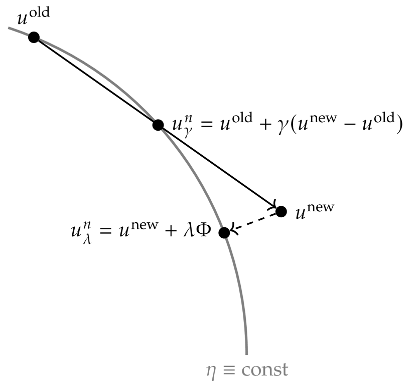
(a) Conservative problem, anti-dissipative method.

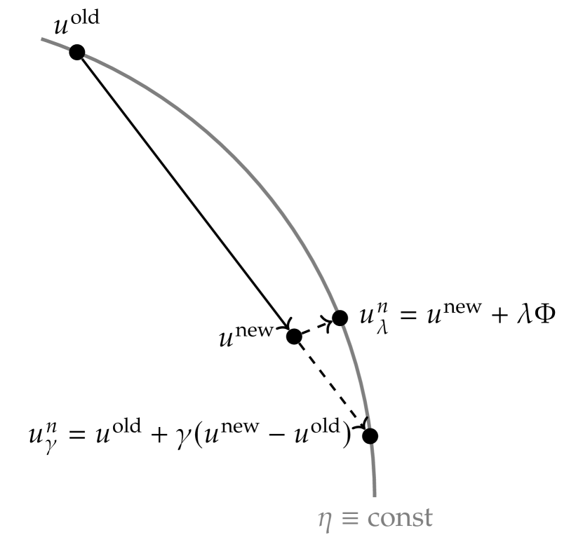
(b) Conservative problem, dissipative method.

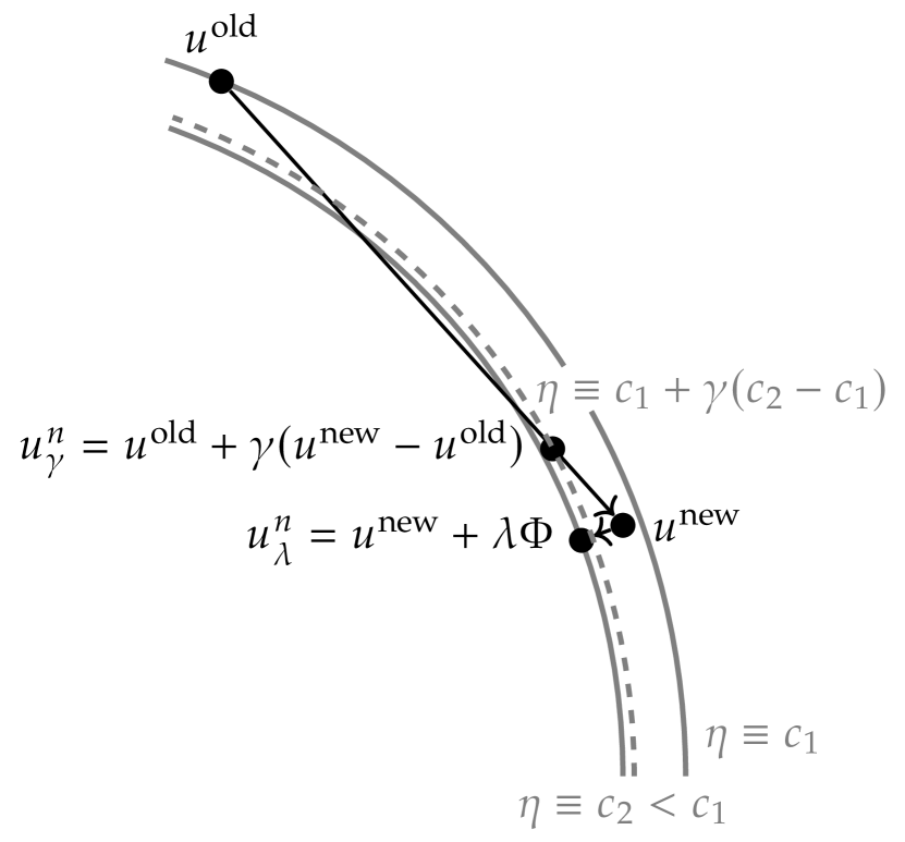
(c) Dissipative problem, anti-dissipative method.

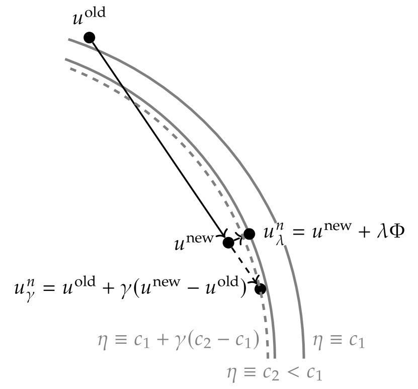
(d) Dissipative problem, dissipative method.

Figure 1: Visualization of the orthogonal projection and relaxation approaches for conservative/dissipative problems and anti-dissipative/dissipative time integration methods for $m=1$ in (12).

Remark 2.5.

Based on the sketches shown in Figure 1, one can expect that it is also possible to choose $\widetilde{\gamma}$ such that $\eta(u^{n}_{\widetilde{\gamma}})=\eta^{\mathrm{new}}$ for dissipative problems. At least for convex problems visualized there, there will be two solutions $\widetilde{\gamma}$ for sufficiently small time steps $\Delta t$. One of these solutions is near unity and the other one is closer to zero.

In order to solve $\eta(u^{n}_{\widetilde{\gamma}})=\eta^{\mathrm{new}}$, $\widetilde{\gamma}$ must deviate more from unity than a solution $\gamma$ of $\eta(u^{n}_{\gamma})=\mathcal{H}(t^{n}_{\gamma})$, cf. (11). Since $\gamma=1+\mathcal{O}(\Delta t^{p-1})$ for a $p$th order baseline scheme as will be shown below, $\widetilde{\gamma}$ cannot be closer to unity than $\mathcal{O}(\Delta t^{p-1})$. In the following, we will prove

$$u^{n}_{\gamma}=u(t^{\mathrm{new}})+\mathcal{O}(\Delta t^{p-1})\quad\text{and}\quad u^{n}_{\gamma}=u(t^{n}_{\gamma})+\mathcal{O}(\Delta t^{p+1}).$$ (16)

Hence, $\eta^{\mathrm{new}}$ is only an $\mathcal{O}(\Delta t^{p-1})$ approximation at $t^{n}_{\gamma}$ and cannot be better at $t^{n}_{\widetilde{\gamma}}$. Thus, solving $\eta(u^{n}_{\widetilde{\gamma}})=\eta^{\mathrm{new}}$ will lead to some order reduction and is not pursued further.

Following the development of the relaxation approach for Runge–Kutta methods [32, 54], the accuracy and suitability of general relaxation time integration methods is studied in three steps. Firstly, accuracy of the relaxed approximation (13) is studied given assumptions on the relaxation parameter $\gamma\approx 1$. Secondly, existence and accuracy of a suitable relaxation parameter $\gamma$ satisfying (11) is studied at first for convex $\eta$ and then for general $\eta$. Finally, methods for computing $\eta^{\mathrm{new}}$ are given.

2.1 Accuracy of the Solution $u$ for Relaxation Methods

Before proving the accuracy of $u^{n}_{\gamma}$, we introduce the following

Lemma 2.6.

For a smooth function $\varphi$, define

$$\varphi^{\mathrm{old}}=\sum_{i=0}^{m-1}\nu_{i}\varphi(u^{n-m+i}),$$ (17)

where $\nu_{i}$ and $m$ are as in (12). Then, $\varphi^{\mathrm{old}}=\varphi(u^{\mathrm{old}})+\mathcal{O}(\Delta t^{2})$.

Proof.

Consider the expansions

$$\varphi^{\mathrm{old}}=\sum_{i=0}^{m-1}\nu_{i}\varphi(u^{n-m+i})=\sum_{i=0}^{m-1}\nu_{i}\left(\varphi(u^{n-m})+\varphi^{\prime}(u^{n-m})(u^{n-m+i}-u^{n-m})\right)+\mathcal{O}(\Delta t^{2})$$ (18)

and

$$\varphi(u^{\mathrm{old}})=\varphi\biggl{(}\sum_{i=0}^{m-1}\nu_{i}u^{n-m+i}\biggr{)}=\varphi(u^{n-m})+\varphi^{\prime}(u^{n-m})\biggl{(}\sum_{i=0}^{m-1}\nu_{i}u^{n-m+i}-u^{n-m}\biggr{)}+\mathcal{O}(\Delta t^{2}).$$ (19)

Because of $\sum_{i}\nu_{i}=1$, we have $\varphi^{\mathrm{old}}-\varphi(u^{\mathrm{old}})=\mathcal{O}(\Delta t^{2})$. ∎

Note that in general

$$u^{\mathrm{old}}=\sum_{i=0}^{m-1}\nu_{i}u^{n-m+i} =\sum_{i=0}^{m-1}\nu_{i}u(t^{n-m+i})+\mathcal{O}(\Delta t^{p+1})$$ (20)

$$\neq u\biggl{(}\sum_{i=0}^{m-1}\nu_{i}t^{n-m+i}\biggr{)}+\mathcal{O}(\Delta t^{p+1})=u(t^{\mathrm{old}})+\mathcal{O}(\Delta t^{p+1}),$$

except for $m=1$ or similarly special choices of $\nu=(\nu_{i})_{i}$. In general, $u^{\mathrm{old}}=u(t^{\mathrm{old}})+\mathcal{O}(\Delta t^{2})$.

Lemma 2.7.

If the method (5) is of order $p\geq 2$ and $\gamma=1+\mathcal{O}(\Delta t^{p-1})$, the relaxation solution (13) is also of order $p$.

Proof.

Use the accuracy of the baseline method (5) and apply Lemma 2.6 to get the expansion

$$u^{n}_{\gamma} =u^{\mathrm{new}}+(\gamma-1)(u^{\mathrm{new}}-u^{\mathrm{old}})$$ (21)

$$=u(t^{\mathrm{new}})+(\gamma-1)\bigl{(}u(t^{\mathrm{new}})-u(t^{\mathrm{old}})\bigr{)}+\mathcal{O}(\Delta t^{p+1})+\mathcal{O}\bigl{(}(\gamma-1)\Delta t^{2}\bigr{)}$$

$$=u(t^{\mathrm{new}})+u^{\prime}(t^{\mathrm{new}})(\gamma-1)(t^{\mathrm{new}}-t^{\mathrm{old}})+\mathcal{O}(\Delta t^{p+1})+\mathcal{O}\bigl{(}(\gamma-1)\Delta t^{2}\bigr{)}.$$

Subtracting the Taylor expansion

$$u(t^{n}_{\gamma}) =u(t^{\mathrm{new}}+(\gamma-1)(t^{\mathrm{new}}-t^{\mathrm{old}}))$$ (22)

$$=u(t^{\mathrm{new}})+u^{\prime}(t^{\mathrm{new}})(\gamma-1)(t^{\mathrm{new}}-t^{\mathrm{old}})+\mathcal{O}\bigl{(}(\gamma-1)^{2}\Delta t^{2}\bigr{)}$$

results in the estimate

$$u^{n}_{\gamma}-u(t^{n}_{\gamma})=\mathcal{O}(\Delta t^{p+1})+\mathcal{O}\bigl{(}(\gamma-1)^{2}\Delta t^{2}\bigr{)}+\mathcal{O}\bigl{(}(\gamma-1)\Delta t^{2}\bigr{)}=\mathcal{O}(\Delta t^{p+1}).$$ (23)

∎

Remark 2.8.

This basic argument (for $m=1$, i.e. $u^{\mathrm{old}}=u^{n-1}$) proves also the accuracy of relaxation Runge–Kutta methods if $\gamma=1+\mathcal{O}(\Delta t^{p-1})$; cf. [32, 54]. In particular, it simplifies the proof of [32, Theorem 2.7] by avoiding the usual Runge–Kutta order conditions. In addition, the result holds also for more general schemes such as the class of general linear methods [8] or (modified) Patankar–Runge–Kutta methods [5].

2.2 Existence and Accuracy of $\gamma$ for Relaxation Methods for Convex Entropies

Lemma 2.9.

Consider a relaxation method (13) based on a time integration method of order $p\geq 2$.

If $\eta$ is a convex entropy for the ODE (1), $\Delta t$ is sufficiently small, and $\eta^{\prime\prime}(u^{\mathrm{old}})\bigl{(}f(u^{\mathrm{old}}),f(u^{\mathrm{old}})\bigr{)}\neq 0$, then there is a unique $\gamma>0$ that solves (13). This $\gamma$ satisfies $\gamma=1+\mathcal{O}(\Delta t^{p-1})$.

Proof.

The function $r$ defined in a neighborhood of $[0,1]$ by

$$r(\gamma) =\eta(u^{n}_{\gamma})-\mathcal{H}(t^{n}_{\gamma})$$ (24)

$$=\eta\bigl{(}u^{\mathrm{old}}+\gamma(u^{\mathrm{new}}-u^{\mathrm{old}})\bigr{)}-\eta^{\mathrm{old}}-\gamma\bigl{(}\eta^{\mathrm{new}}-\eta^{\mathrm{old}}\bigr{)}$$

is convex, since $\eta$ is convex. Moreover,

$$r(0)=\eta(u^{\mathrm{old}})-\eta^{\mathrm{old}}=\eta\biggl{(}\sum_{i=0}^{m-1}\nu_{i}u^{n-m+i}\biggr{)}-\sum_{i=0}^{m-1}\nu_{i}\eta(u^{n-m+i})\leq 0,$$ (25)

since $u^{\mathrm{old}}$ is a convex combination and $\eta$ is convex. Furthermore,

$$r^{\prime}(0) =\eta^{\prime}(u^{\mathrm{old}})(u^{\mathrm{new}}-u^{\mathrm{old}})-\eta^{\mathrm{new}}+\eta^{\mathrm{old}}$$ (26)

$$=\eta^{\mathrm{old}}-\eta(u^{\mathrm{new}})+\eta^{\prime}(u^{\mathrm{old}})(u^{\mathrm{new}}-u^{\mathrm{old}})+\mathcal{O}(\Delta t^{p+1}).$$

Because of

$$\sum_{i=0}^{m-1}\nu_{i}\eta^{\prime}(u^{n-m+i})=\eta^{\prime}(u^{\mathrm{old}})+\mathcal{O}(\Delta t^{2}),$$ (27)

cf. Lemma 2.6, we have

$$r^{\prime}(0) =-\frac{1}{2}\eta^{\prime\prime}(u^{\mathrm{old}})(u^{\mathrm{new}}-u^{\mathrm{old}},u^{\mathrm{new}}-u^{\mathrm{old}})+\mathcal{O}(\Delta t^{3})$$ (28)

$$=-\frac{1}{2}(t^{\mathrm{new}}-t^{\mathrm{old}})^{2}\eta^{\prime\prime}(u^{\mathrm{old}})(f(u^{\mathrm{old}}),f(u^{\mathrm{old}}))+\mathcal{O}(\Delta t^{3})<0$$

for sufficiently small $\Delta t>0$. Here, the accuracy of the estimate (10) has been used in the second line. Similarly,

$$r^{\prime}(1) =\eta^{\prime}(u^{\mathrm{new}})(u^{\mathrm{new}}-u^{\mathrm{old}})-\eta^{\mathrm{new}}+\eta^{\mathrm{old}}$$ (29)

$$=\eta^{\mathrm{old}}-\eta(u^{\mathrm{new}})-\eta^{\prime}(u^{\mathrm{new}})(u^{\mathrm{old}}-u^{\mathrm{new}})+\mathcal{O}(\Delta t^{p+1})$$

$$=\frac{1}{2}\eta^{\prime\prime}(u^{\mathrm{new}})(u^{\mathrm{old}}-u^{\mathrm{new}},u^{\mathrm{old}}-u^{\mathrm{new}})+\mathcal{O}(\Delta t^{3})$$

$$=\frac{1}{2}(t^{\mathrm{new}}-t^{\mathrm{old}})^{2}\eta^{\prime\prime}(u^{\mathrm{new}})(f(u^{\mathrm{old}}),f(u^{\mathrm{old}}))+\mathcal{O}(\Delta t^{3})>0$$

for sufficiently small $\Delta t>0$. Hence, $r$ has a unique positive root $\gamma$.

Because of the accuracy of the baseline scheme, $r(1)=\mathcal{O}(\Delta t^{p+1})$. Using (29), $r^{\prime}(1)=c\Delta t^{2}+\mathcal{O}(\Delta t^{3})$ with $c>0$. Hence, the root $\gamma$ of $r$ satisfies $\gamma=1+\mathcal{O}(\Delta t^{p-1})$. ∎

Remark 2.10.

Instead of the condition $\eta^{\prime\prime}(u^{\mathrm{old}})\bigl{(}f(u^{\mathrm{old}}),f(u^{\mathrm{old}})\bigr{)}\neq 0$, similar conditions using other step/stage values can be used by performing the Taylor expansions around them.

Remark 2.11.

As can be seen from Figure 1, choosing $\gamma$ slightly smaller than the root of $r(\gamma)=0$ is a way to introduce additional dissipation.

Remark 2.12.

If the convex entropy is a squared inner-product norm, i.e. if $\eta(u)=\frac{1}{2}\|u\|^{2}$ in a Hilbert space, the relaxation parameter can be calculated explicitly as

$$\gamma=\begin{dcases}\frac{-b+\sqrt{b^{2}-4ac}}{2c},&a\neq 0,\\ \frac{-b}{c},&a=0,\end{dcases}$$ (30)

where

$$\begin{gathered}a=\eta(u^{\mathrm{old}})-\eta^{\mathrm{old}}\leq 0,\qquad b=\left\langle{u^{\mathrm{old}},\,u^{\mathrm{new}}-u^{\mathrm{old}}}\right\rangle-\eta^{\mathrm{new}}+\eta^{\mathrm{old}},\\ c=\eta(u^{\mathrm{new}}-u^{\mathrm{old}})\geq 0.\end{gathered}$$ (31)

Theorem 2.13.

Consider a relaxation method (13) based on a time integration method of order $p\geq 2$.

If $\eta$ is a convex entropy for the ODE (1), $\Delta t$ is sufficiently small, and $\eta^{\prime\prime}(u^{\mathrm{old}})\bigl{(}f(u^{\mathrm{old}}),f(u^{\mathrm{old}})\bigr{)}\neq 0$, then there is a unique $\gamma>0$ that satisfies the relaxation condition (11) and the resulting relaxation method is of order $p$.

Proof.

Combine Lemma 2.7 and Lemma 2.9. ∎

2.3 Existence and Accuracy of $\gamma$ for Relaxation Methods for General Functionals

Theorem 2.14.

Consider a relaxation method (13) based on a time integration method of order $p\geq 2$. If $\eta$ is a general (i.e. not necessarily convex) smooth functional of (1), $\Delta t$ is sufficiently small, and

$$\eta^{\prime}(u^{\mathrm{new}})\frac{u^{\mathrm{new}}-u^{\mathrm{old}}}{\|u^{\mathrm{new}}-u^{\mathrm{old}}\|}=c\Delta t+\mathcal{O}(\Delta t^{2}),\quad\text{with }c\neq 0,$$ (32)

then there is a unique $\gamma=1+\mathcal{O}(\Delta t^{p-1})$ that satisfies the relaxation condition (11) and the resulting relaxation method is of order $p$.

Proof.

Following [10, Theorem 2], this proof is based on the implicit function theorem, e.g. the version of [55, Section VIII.2].

Given an initial condition $u^{0}$ and a time step $\Delta t$, approximate solutions $u^{n-k+i}\approx u(t^{n-k+i})$ and $u^{\mathrm{new}}\approx u(t^{\mathrm{new}})$ are computed, e.g. via a (relaxation) LMM and a suitable starting procedure. In this setting, the proof of [10, Theorem 2] can be adapted, similarly to [54, Proposition 2.18], yielding a unique solution $\gamma=1+\mathcal{O}(\Delta t^{p-1})$. Because of Lemma 2.7, the relaxation method is of order $p$. ∎

Remark 2.15.

For one-step methods studied in [32, 54, 52], the natural choice of $m,\nu$ in (12) is $m=1$ and $\nu_{i}=\delta_{i,0}$, where $\delta_{i,0}$ is the Kronecker delta. Then, $r(0)=0$ in (24).

3 Suitable Estimates of $\eta$ for Relaxation Methods

For dissipative systems, the relaxation approach requires an estimate of the entropy at $t^{\mathrm{new}}$ satisfying

$$\eta^{\mathrm{new}}\leq\eta^{\mathrm{old}}$$ (33)

in order to ensure that (3) is satisfied if $m\leq k$. We first review the approach of [54] for Runge–Kutta methods with positive weights, showing how it fits naturally into the approach we have just described. We then discuss how to obtain a suitable estimate for multistep methods with positive coefficients, and for more general methods.

3.1 Runge–Kutta Methods with Positive Quadrature Weights

A Runge–Kutta method with $s$ stages takes the form [8, 26]

$$y^{i} =u^{n-1}+\Delta t\sum_{j=1}^{s}a_{ij}\,f(t^{n-1}+c_{j}\Delta t,y^{j}),\qquad i\in\left\{1,\dots,s\right\},$$ (34a)

$$u^{\mathrm{new}} =u^{n-1}+\Delta t\sum_{i=1}^{s}b_{i}\,f(t^{n-1}+c_{i}\Delta t,y^{i}).$$ (34b)

Given the Runge–Kutta stage values, a natural estimate $\eta^{\mathrm{new}}$ is given by using the quadrature rule of the Runge–Kutta method itself:

$$\eta^{\mathrm{new}}=\eta(u^{n-1})+\Delta t\sum_{i=1}^{s}b_{i}(\eta^{\prime}f)(y^{i}).$$ (35)

This corresponds to the approach used in [15, 9, 32, 54]. The inequality (33) is guaranteed if the weights $b_{i}\geq 0$.

Remark 3.1.

The adaptation of the time $t^{n}_{\gamma}$ and this choice of the estimate appear to be very natural. Indeed, considering the augmented system

$$\dfrac{\operatorname{d\!}{}}{\operatorname{d\!}{t}}\begin{pmatrix}t\\ u(t)\\ \eta(u(t))\end{pmatrix}=\begin{pmatrix}1\\ f(u(t))\\ (\eta^{\prime}f)(u(t))\end{pmatrix},$$ (36)

the update formula (with $\sum_{i}b_{i}=1$)

$$\begin{pmatrix}t^{n}_{\gamma}\\ u^{n}_{\gamma}\\ \eta(u^{n}_{\gamma})\end{pmatrix}=\begin{pmatrix}t^{n-1}\\ u^{n-1}\\ \eta(u^{n-1})\end{pmatrix}+\gamma\Delta t\sum_{i=1}^{s}b_{i}\begin{pmatrix}1\\ f(y^{i})\\ (\eta^{\prime}f)(y^{i})\end{pmatrix}$$ (37)

is a natural discretization of (36), where the relaxation parameter $\gamma$ is introduced to enforce the consistent evolution of $\eta$.

Remark 3.2.

In the context of dissipative PDEs such as second-order parabolic ones, (35) can provide important (spatial) gradient estimates of the stage/step values by bounding $\eta^{\prime}f$.

3.2 Linear Multistep Methods with Positive Coefficients

A linear multistep method can be written in the form

$$u^{\mathrm{new}}=\sum_{i=0}^{k-1}\alpha^{n}_{i}u^{n-k+i}+\Delta t\sum_{i=0}^{k}\beta^{n}_{i}f^{n-k+i}.$$ (38)

The coefficients $\alpha^{n}_{i},\beta^{n}_{i}$ have a time index because they depend on the sequence of step sizes. If all coefficients $\alpha^{n}_{i},\beta^{n}_{i}$ are non-negative, the method itself can be used to obtain a suitable estimate $\eta^{\mathrm{new}}$. Indeed, considering again the augmented system (36), a high-order estimate is obtained as

$$\eta^{\mathrm{new}}=\sum_{i\geq 0}\left(\alpha^{n}_{i}\eta(u^{n-k+i})+\Delta t\beta^{n}_{i}(\eta^{\prime}f)(u^{n-k+i})\right)=\eta(u^{\mathrm{new}})+\mathcal{O}(\Delta t^{p+1}).$$ (39)

Since $\sum_{i}\alpha^{n}_{i}=1$ for any consistent method and $\beta^{n}_{i}(\eta^{\prime}f)(u^{n-k+i})\leq 0$, the dissipation condition (33) is guaranteed. Note in particular that strong stability preserving (SSP) LMMs have non-negative coefficients [22, Chapter 8] and can be used in this manner.

3.3 General Time Integration Methods

The approach of the previous two subsections relies on non-negativity of the coefficients $b_{i}$ and $\alpha_{i},\beta_{i}$, respectively. For methods with negative coefficients, we can follow the technique developed in [10]. In this approach, an estimate $\eta^{\mathrm{new}}$ is obtained by interpolation (continuous/dense output) and a positive quadrature rule. Indeed, consider a quadrature rule of order at least $p$ with nodes $\tau_{i}\in[t^{n-m},t^{\mathrm{new}}]$ and positive weights $w_{i}$, e.g. a Gauß quadrature. Compute an interpolant $y(\tau_{i})$ of order at least $p-1$ at the nodes and use

$$\eta^{\mathrm{new}}=\eta^{n-m}+\sum_{i}w_{i}(\eta^{\prime}f)(y(\tau_{i})).$$ (40)

Because $w_{i}>0$, the estimate is guaranteed to satisfy (33) for dissipative systems.

In contrast to the previous method, this approach requires additional evaluations of $\eta^{\prime}$ and $f$ at the intermediate values and is thus more costly. On the other hand, it can be applied to general time integration methods and does not require any special structure (besides a continuous output formula). In particular, it is not limited to Runge–Kutta or linear multistep methods.

Remark 3.3.

This approach is particularly interesting for linear multistep methods, since these schemes are often defined naturally in terms of (interpolating) polynomials [2, 40].

4 Relaxation Linear Multistep Methods With Fixed Coefficients

Since orthogonal projection does not inherently involve any change in the step size, it can be used with a fixed step size. In contrast, relaxation methods necessarily introduce variation in the step size, due to the parameter $\gamma$, even if the intended $\Delta t$ at each step is constant. To make use of Theorems 2.13 and 2.14 to guarantee high-order accuracy, multistep relaxation methods must be implemented in a way that takes into account the variation in the step size. On the other hand, since $\gamma$ is very close to unity, this step-size variation is quite small. Thus it is interesting to know what accuracy may be obtained by relaxation methods using the new time step (7b) but implemented with the coefficients of the corresponding fixed step size method. We will write simply $\alpha_{i},\beta_{i}$ (without superscripts) to refer to the coefficients of a fixed step size LMM.

Theorem 4.1.

Given a $k$-step LMM (38) of order $p\geq 1$ with coefficients $(\alpha,\beta)$, suppose that the method is used with step sizes $\Delta t_{n-k+j}=\gamma_{j}\Delta t_{n}$, where $\gamma_{j}-1=\mathcal{O}(\Delta t^{q})$ but the coefficients are not adapted. Then the one-step error is $\mathcal{O}(\Delta t^{\min(p+1,q+1)})$. Furthermore, for Adams methods the one-step error is $\mathcal{O}(\Delta t^{\min(p+1,q+2)})$.

Proof.

The one-step error takes the form [36, p. 133], [24, Eqn. (2.16)]

$$E =\sum_{\ell=0}^{\infty}\Delta t^{\ell}u^{(\ell)}(t^{\mathrm{new}})C_{\ell}(\alpha,\beta,\gamma)$$ (41)

where $C_{0}=\sum_{j}\alpha_{j}-1$ and for $\ell>0$

$$C_{\ell}(\alpha,\beta,\gamma)=\sum_{j=0}^{k-1}\left(\Omega_{j}^{\ell}\alpha_{j}+\ell\Omega_{j}^{\ell-1}\beta_{j}\right)-\Omega_{k}^{\ell}$$ (42)

with

$$\Omega_{j} =\sum_{i=1}^{j}\frac{\Delta t_{n-k+i}}{\Delta t_{n}}=\sum_{i=1}^{j}\gamma_{j}=j+\sum_{i=1}^{j}(\gamma_{j}-1)=j+\delta_{j},$$ (43)

where $\delta_{j}=\mathcal{O}(\Delta t^{q})$. Since the LMM has order $p$, its coefficients satisfy the fixed step size order conditions $C_{0}=0$ and

$$C_{\ell}^{\text{unif}}\mathrel{\mathop{\ordinarycolon}}=C_{\ell}(\alpha,\beta,\mathbbm{1})=\sum_{j=0}^{k-1}\left(j^{\ell}\alpha_{j}+\ell j^{\ell-1}\beta_{j}\right)-k^{\ell} =0, \ell\in\{1,2,\dots,p\}.$$ (44)

Subtracting (44) from (42) shows that $C_{\ell}=\mathcal{O}(\Delta t^{q})$ for $1\leq\ell\leq p$. Substitution into (41) gives the result stated in the first part of the theorem. For the second result, observe that

$$C_{1}(\alpha,\beta,\gamma) =\sum_{j=0}^{k-1}\left((j+\delta_{j})\alpha_{j}+\beta_{j}\right)-k-\delta_{k}$$ (45)

$$=C_{1}^{\text{unif}}+\sum_{j=0}^{k-1}(\delta_{j}\alpha_{j})-\delta_{k}=\sum_{j=0}^{k-1}(\delta_{j}\alpha_{j})-\delta_{k}.$$ (46)

Since $\gamma_{k}=1$, we have $\delta_{k}=\delta_{k-1}$. For Adams methods we have $\alpha_{k-1}=1$, while $\alpha_{j}=0$ for $j\neq k-1$, so $C_{1}(\alpha,\beta,\gamma)=0$. ∎

Note that in the theorem we have analyzed the accuracy of $u^{\mathrm{new}}$ rather than that of $u^{n}_{\gamma}$, but the proof of Lemma 2.7 shows that $u^{n}_{\gamma}$ will have the same order of accuracy. According to Lemma 2.9, the assumption in the theorem is fulfilled for relaxation methods with $q=p-1$. This suggests that (for non-Adams methods) the local error in the first step will be one order worse than the design order of the method. But then for the next step Lemma 2.9 shows that $\gamma-1$ will also be one order worse. In this manner, the local error can grow by one order at each step, until very quickly all accuracy is lost and/or a suitable solution $\gamma>0$ cannot be found. We see that Adams methods are free from this problem. A cure for this problem for another classes of LMMs is discussed next.

Consider a linear multistep method (38) with non-negative coefficients $\alpha_{i}$ and take the special choice $\nu_{i}=\alpha_{i}$ for computing the old values in (12). This yields

$$\begin{pmatrix}t^{\mathrm{new}}\\ u^{\mathrm{new}}\end{pmatrix}-\begin{pmatrix}t^{\mathrm{old}}\\ u^{\mathrm{old}}\end{pmatrix}=\Delta t\sum_{i=0}^{k}\beta_{i}\begin{pmatrix}1\\ f^{n-k+i}\end{pmatrix}.$$ (47)

Instead of scaling the time step, this relaxation method can be interpreted as scaling the right hand side of the augmented ODE (36) by introducing the pseudotime $\tau$ with constant time steps $\Delta\tau$ and solving

$$\dfrac{\operatorname{d\!}{}}{\operatorname{d\!}{\tau}}\begin{pmatrix}t(\tau)\\ u(\tau)\\ \eta(u(\tau))\end{pmatrix}=\Gamma(\tau)\begin{pmatrix}1\\ f(u(\tau))\\ (\eta^{\prime}f)(u(\tau))\end{pmatrix},\qquad\dfrac{\operatorname{d\!}{}}{\operatorname{d\!}{\tau}}\Gamma(\tau)=\gamma(\tau),$$ (48)

where $\gamma(\tau)$ is the relaxation parameter. If $\Gamma$ is continuous and bounded away from zero, this new augmented ODE (48) results from (36) by the variable transformation

$$t(0)=0,\qquad\dfrac{\operatorname{d\!}{}t(\tau)}{\operatorname{d\!}{\tau}}=\Gamma(\tau).$$ (49)

Using this interpretation (and choice of $\nu_{i}$), relaxation LMMs with $\alpha_{i}\geq 0$ can also be used with fixed coefficients.

Theorem 4.2.

Consider a fixed coefficient linear multistep method (38) of order $p\geq 2$ with non-negative coefficients $\alpha_{i}\geq 0$ and the corresponding relaxation method (13) with $\nu_{i}=\alpha_{i}$. If $\eta$ is a smooth functional of (1), $\Delta t$ is sufficiently small, and the non-degeneracy condition of Theorem 2.13 (if $\eta$ is convex) or Theorem 2.14 (for general $\eta$) is satisfied, then there is a solution $\gamma$ of (13) and the resulting relaxation method is of order $p$.

Proof.

Since the fixed step size method is of order $p\geq 2$, Theorem 2.13 (if $\eta$ is convex) or Theorem 2.14 (for general $\eta$) can be applied. Hence, there is a solution $\gamma(\tau)=1+\mathcal{O}(\Delta\tau^{p-1})$ of (13).

Because of the special choice of $\nu_{i}=\alpha_{i}$, the sequence of the relaxation solutions is a $p$th order approximation to the solution of (48). Hence, it is also a $p$th order approximation of the solution of (1). ∎

Remark 4.3.

Because of the scaling by $\Gamma(\tau)$ in (48), the relaxation parameter $\gamma$ may be further than expected from unity. Indeed, $\gamma(\tau)=1+\mathcal{O}(\Delta\tau^{p-1})$ yields $\Gamma(\tau^{\mathrm{final}})=1+\mathcal{O}(\Delta\tau^{p-2})$, since $\mathcal{O}(\Delta\tau^{-1})$ time steps have to be used. Hence, the observed alteration of the physical time $t$ is $\max_{\tau}|\Gamma(\tau)\gamma(\tau)-1|=\mathcal{O}(\Delta\tau^{p-2})$.

Remark 4.4.

A relaxation LMM (13) with adapted coefficients is typically more accurate than the same relaxation LMM with fixed coefficients, in particular for second-order methods. Indeed, the factor $\Gamma(\tau)$ in the underlying ODE (48) grows as $\Gamma(\tau)=1+\mathcal{O}(\Delta\tau^{p-2})$. Hence, it does not decrease in size if $\Delta\tau$ is reduced for $p=2$. Since an increase of $\Gamma(\tau)$ results in an increase of the Lipschitz constant of the underlying ODE (48), it is reasonable to expect bigger errors compared to a relaxation method with adapted coefficients solving (36).

5 Stability and Accuracy Properties of Relaxation Methods

Since the relaxation parameter $\gamma=1+\mathcal{O}(\Delta t^{p-1})$ introduces only a small variation of the baseline time integration scheme, basic stability properties are often not lost, similarly to the case of relaxation Runge–Kutta methods [32, Section 3]. Furthermore, applying relaxation can increase the accuracy of baseline schemes.

The incremental direction technique (IDT) approach is basically the relaxation approach without adapting the new time to (7b). For Runge–Kutta methods, this results in a slight loss of the order of accuracy [9, 32, 54], i.e. the IDT method is of order $p-1$. For some LMMs and conservative/dissipative problems, IDT versions result in $\gamma=1+\mathcal{O}(\Delta t^{p-2})$ and an order of accuracy $p-2$. However, there are also dissipative problems where IDT versions fail because no solution for $\gamma$ can be found.

5.1 Zero-Stability of Relaxation Linear Multistep Methods

In general, proving even zero-stability of LMMs with variable step sizes is not easy [63]. Typically, stability of variable step size LMMs is implied if the corresponding fixed step size method has certain stability properties and the step sizes do not vary too much, cf. e.g. [26, Theorems III.5.5 and III.5.7] or [2]. For relaxation LMMs, the step sizes are chosen via the relaxation coefficient $\gamma=1+\mathcal{O}(\Delta t^{p-1})$. Hence, the step sizes vary as

$$\frac{\Delta t_{n}}{\Delta t_{n-1}}=\frac{\gamma_{n}\Delta t}{\gamma_{n-1}\Delta t}=1+\mathcal{O}(\Delta t^{p-1}).$$ (50)

Thus, under the usual conditions, relaxation LMMs are stable if the time step is small enough.

5.2 Strong Stability Preserving Methods

SSP methods with SSP coefficient ${\mathcal{C}}>0$ guarantee a given convex stability property under a time step restriction $\Delta t\leq{\mathcal{C}}\Delta t_{\mathrm{FE}}$ whenever the explicit Euler method satisfies the same convex stability property under the time step restriction $\Delta t\leq\Delta t_{\mathrm{FE}}$; cf. [22] and the references cited therein.

If the relaxation parameter $\gamma\in[0,1]$, then $u^{n}_{\gamma}$ is a convex combination of $u^{\mathrm{new}}$ and $u^{\mathrm{old}}$. Hence, all convex stability properties satisfied by these two values are retained. However, if $\gamma>1$, $u^{n}_{\gamma}$ is not a convex combination and the SSP property with the same SSP coefficient ${\mathcal{C}}$ can be lost, cf. [32, Theorem 3.3 and Table 1], where also more detailed investigations of the SSP property of relaxation Runge–Kutta methods can be found. Specifically, therein it was proved that the SSP coefficient of a relaxation RK method is not smaller than that of the original RK method if

$$0\leq\gamma\leq\frac{-1}{R(-{\mathcal{C}})-1}\geq 1,$$ (51)

where $R$ is the stability function of the explicit SSP Runge–Kutta method (34). We also have the following

Theorem 5.1.

Consider an explicit SSP Runge–Kutta method (34) with SSP coefficient ${\mathcal{C}}$. The corresponding relaxation RK method (13) with $m=1$ has SSP coefficient ${\mathcal{C}}_{\gamma}={\mathcal{C}}+\mathcal{O}(\Delta t^{p-1})$.

Proof.

The stability function $R$ of an $s$-stage Runge–Kutta method with Butcher coefficients $A,b$ is

$$R(z)=1+zb^{T}(\operatorname{I}-zA)^{-1}\mathbbm{1},$$ (52)

where $\mathbbm{1}=(1,\dots,1)^{T}\in\mathbb{R}^{s}$. The stability function of the relaxation method is given by $R_{\gamma}(z)=1+\gamma(R(z)-1)$. The relaxation method is SSP with SSP coefficient $\geq{\mathcal{C}}_{\gamma}$ if $R_{\gamma}(-{\mathcal{C}}_{\gamma})\geq 0$, cf. [32, Lemma 3.2 and Theorem 3.3]. Because $\gamma=1+\mathcal{O}(\Delta t^{p-1})$, this implies $R_{\gamma}(-{\mathcal{C}})=R(-{\mathcal{C}})+\mathcal{O}(\Delta t^{p-1})$. ∎

Let us turn now to linear multistep methods. To maintain the SSP property when the step size is not fixed, we require that any coefficients of the fixed step size method that are equal to zero remain exactly zero when the step size is varied:

$$\alpha_{i} =0\implies\alpha^{n}_{i}=0,$$ (53a)

$$\beta_{i} =0\implies\beta^{n}_{i}=0.$$ (53b)

This assumption is satisfied by the methods of [24, 40]:

Theorem 5.2.

Consider an explicit SSP LMM (38) with SSP coefficient ${\mathcal{C}}$ and satisfying (53). If $m$ and $\nu_{i}$ are chosen such that $\nu_{i-m}>0\implies\alpha_{i-k}>0$, then for small enough $\Delta t$ the relaxation LMM (13) is SSP with an SSP coefficient ${\mathcal{C}}_{\gamma}={\mathcal{C}}+\mathcal{O}(\Delta t^{p-1})$ and ${\mathcal{C}}_{\gamma}\geq{\mathcal{C}}$ if $\gamma\in[0,1]$. Furthermore, if $m=k$ and $\nu_{i}=\alpha^{n}_{i}$ then ${\mathcal{C}}_{\gamma}={\mathcal{C}}/\gamma$.

Proof.

Here, we use the definition of the SSP coefficient given as ${\mathcal{C}}_{n}$ in [24], which can be written as

$${\mathcal{C}}=\begin{cases}\max\left\{r\in[0,\infty)\;\middle|\;\forall i\colon\alpha_{i}-r\beta_{i}\geq 0\right\},&\text{if }\forall i\colon\alpha_{i},\beta_{i}\geq 0,\\ 0,&\text{otherwise}.\end{cases}$$ (54)

The relaxation LMM can be interpreted as an LMM with parameters

$$\alpha_{i,\gamma}=\nu_{i}(1-\gamma)+\gamma\alpha_{i},\quad\text{and}\quad\beta_{i,\gamma}=\gamma\beta_{i}.$$ (55)

Using $\gamma=1+\mathcal{O}(\Delta t^{p-1})$, $\alpha_{i,\gamma}=\alpha_{i}+\mathcal{O}(\Delta t^{p-1})$ and $\beta_{i,\gamma}=\beta_{i}+\mathcal{O}(\Delta t^{p-1})$. For small enough $\Delta t$ these coefficients are also non-negative. Hence, ${\mathcal{C}}_{\gamma}={\mathcal{C}}+\mathcal{O}(\Delta t^{p-1})$.

Meanwhile, if $m=k$ and $\nu_{i}=\alpha_{i}$ then the relaxation LMM can be written as a standard LMM but with coefficients $(\alpha,\gamma\beta)$. Hence the SSP coefficient is ${\mathcal{C}}/\gamma$. ∎

Choosing a variable step size method that does not satisfy the implication $\nu_{i-m}>0\implies\alpha_{i-k}>0$ can lead to loss of the SSP property. For instance, the second-order three-step method with variable step size of [24] is given by

$$u^{\mathrm{new}}=\frac{\Omega_{2}^{2}-1}{\Omega_{2}^{2}}\left(u^{n-1}+\frac{\Omega_{2}}{\Omega_{2}-1}\Delta tf(u^{n-1})\right)+\frac{1}{\Omega_{2}^{2}}u^{n-3},$$ (56)

where $\Omega_{2}=(t^{n-1}-t^{n-3})/\Delta t$. Taking e.g. $m=2$ and $\nu_{0}\neq 0$ generates a term $(1-\gamma)u^{n-2}$ in the relaxation solution, which destroys the SSP property when $\gamma>1$.

In general, orthogonal projection methods can violate SSP properties. Indeed, linear functionals are convex and linear invariants are preserved by the explicit Euler method (as well as by all Runge–Kutta, linear multistep, and general linear methods). Since orthogonal projection methods do not conserve linear invariants in general, the corresponding convex stability property is lost.

Example 5.3.

Consider the two-step second-order SSP Runge–Kutta method SSPRK(2,2) given by

$$y^{1} =u^{n-1},$$ (57)

$$y^{2} =u^{n-1}+\Delta tf(y^{1}),$$

$$u^{\mathrm{new}} =u^{n-1}+\frac{1}{2}\Delta t\left(f(y^{1})+f(y^{2})\right).$$

Solutions $u$ of the ODE

$$\dfrac{\operatorname{d\!}{}}{\operatorname{d\!}{t}}u(t)=\begin{pmatrix}0&-1&1\\ 1&0&-1\\ -1&1&0\end{pmatrix}u(t),\quad u(0)=\begin{pmatrix}-1\\ 0\\ 0\end{pmatrix},$$ (58)

have a constant energy $\eta(u)=\frac{1}{2}\|u\|^{2}$ and total mass $\mathcal{M}(u)=\sum_{i}u_{i}$. The first step of the orthogonal projection SSPRK(2,2) method results in the total mass

$$\mathcal{M}(u^{1}_{\lambda})=-\frac{\sqrt{2}}{\sqrt{2+3\Delta t^{4}}}>\mathcal{M}(u^{0}).$$ (59)

Hence, the convex stability property related to the total mass is violated. In contrast, the relaxation SSPRK(2,2) method preserves the total mass.

6 Numerical Results

Here, the following classes of linear multistep methods (38) are considered. If not stated otherwise, the estimate $\eta^{\mathrm{new}}$ is obtained using a dense output formula and Gauß quadrature using one ($k=2$) or two ($k\in\{3,4\}$) nodes.

• Adams($k$)
  The $k$-step explicit Adams methods (also known as Adams–Bashforth methods) are based on the formula $u^{n}=u^{n-1}+\int_{t^{n-1}}^{t^{n}}\mathcal{P}_{f}$, where $\mathcal{P}_{f}$ is the polynomial interpolating $f(u^{n-1})$, …, $f(u^{n-k})$, see [3] and [26, Section III.1]. These methods can be used with variable step sizes. A natural dense output at an intermediate value $\tau_{i}$ is generated by evaluating the integral with upper limit $\tau_{i}$ instead of $t^{n}$.

• Nyström($k$)AS
  The $k$-step Nyström methods are based on the formula $u^{n}=u^{n-2}+\int_{t^{n-2}}^{t^{n}}\mathcal{P}_{f}$, where $\mathcal{P}_{f}$ is again the polynomial interpolating $f(u^{n-1})$, …, $f(u^{n-k})$, see [42] and [26, Section III.1]. Based on these constant step size Nyström methods, an extension to variable step sizes that is equipped with a dense output formula has been proposed by Arévalo and Söderlind [2] and will be denoted as Nyström($k$)AS.

• eBDF($k$), eBDF($k$)AS
  The family of extrapolated backward difference formula (eBDF) methods is based on the formula $\mathcal{P}_{u}^{\prime}(t^{n})=\mathcal{P}_{f}(t^{n})$, where $\mathcal{P}_{u}$ and $\mathcal{P}_{f}$ are polynomials that interpolate the previous step values $u^{n-i}$ and step derivatives $f(u^{n-i})$, respectively, cf. [56]. Based on the constant step size eBDF methods, an extension to variable step sizes that is equipped with a dense output formula has been proposed by Arévalo and Söderlind [2] and will be denoted as eBDF($k$)AS.

• SSP($k,p$), SSP($k,p$)AS
  Second and third order accurate variable step size SSP LMMs have been proposed in [24]. The estimate of the evolution of $\eta$ can either be based on the evolution predicted by the SSP method itself (39) or on the quadrature (40) using the dense output formula of [40], which is based on the framework of [2]. If the latter option is chosen, the method is denoted as SSP($k,p$)AS.

• EDC($i$,$j$)
  The explicit difference correction (EDC) methods of [1] are extended to variable step sizes and equipped with a dense output using the approach of [2].

• BDF($k$)
  The family of backward difference formula (BDF) methods is based on the formula $p_{u}^{\prime}(t^{n})=f(\mathcal{P}_{u}(t^{n}))$, where $\mathcal{P}_{u}$ is a polynomial that interpolates the step values $u^{n},u^{n-1}$, …, $u^{n-k}$, cf. [12] and [26, Section III.1].

If not stated otherwise, relaxation LMMs have been adapted to the new step sizes using $m=1$ and $\nu_{i}=\delta_{i,0}$ in (12). We have checked that the results using different choices of $\nu_{i}$ are similar. Since Theorem 4.2 can be applied to Adams methods, Nyström methods, and SSP LMMs, we have also tested the corresponding fixed coefficient version of these schemes.

Remark 6.1.

The modified leapfrog method of [57] is the relaxation Nyström($2$)AS method for conservative inner-product norms with $m=2$ and $\nu_{i}=\delta_{i,0}$ in (12) and fixed step sizes, cf. Theorem 4.2.

We have implemented the relaxation methods used in this article in Python, using SciPy [70] to solve the scalar non-quadratic equations for the relaxation parameter $\gamma$. Matplotlib [30] has been used to generate the plots. The source code for all numerical examples is available online [51].

6.1 Nonlinear Oscillator

For the nonlinear oscillator

$$\dfrac{\operatorname{d\!}{}}{\operatorname{d\!}{t}}\begin{pmatrix}u_{1}(t)\\ u_{2}(t)\end{pmatrix}=\|u(t)\|^{-2}\begin{pmatrix}-u_{2}(t)\\ u_{1}(t)\end{pmatrix},\quad u^{0}=\begin{pmatrix}1\\ 0\end{pmatrix},$$ (60)

of [46, 50], the energy $\eta(u)=\frac{1}{2}\|u\|^{2}$ is conserved. We choose this test problem to demonstrate the convergence properties of relaxation methods in a simple setting where the relaxation parameter can also be computed explicitly by solving a quadratic equation. We use some common explicit methods here because this problem is not stiff.

Results of a convergence study for this problem are visualized in Figure 2. The Nyström($k$)AS, $k\in\{3,4\}$, methods result in a large error and are not completely in the asymptotic regime, which could be attributed to their lack of a reasonable stability region [28, Section V.1]. However, applying projection or relaxation results in the expected order of accuracy. The Adams methods do not have similar problems and work well. All other explicit methods described above behave similarly to the Adams methods. For this test problem and formally odd-order relaxation and projection methods, there is a certain superconvergence phenomenon, increasing the experimental order of accuracy by one in accordance with Theorem A.1.

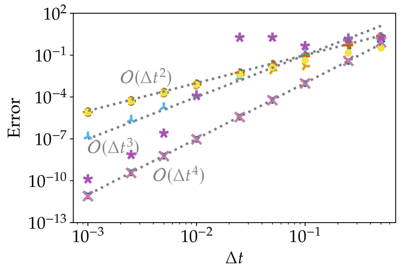
(a) Adams($k$) methods.

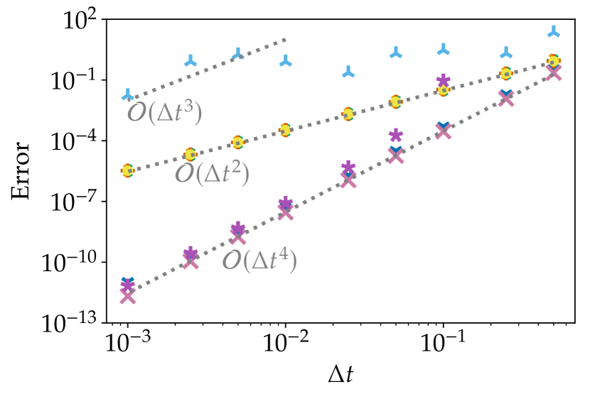
(b) Nyström($k$)AS methods.

Figure 2: Convergence study for linear multistep methods applied to the nonlinear oscillator (60) with final time $t=20$.

The fixed coefficient versions of Adams($3$) and Nyström($3$)AS result in larger errors than the corresponding versions with adapted coefficients. For smaller time steps $\Delta t$, they are even not in the asymptotic regime. This behavior is in accordance with the analysis of Section 4. The energy evolution of a representative example from this section is shown in Figure 4(a).

6.2 Kepler Problem

The Kepler problem

$$\begin{gathered}\dfrac{\operatorname{d\!}{}}{\operatorname{d\!}{t}}q(t)=\dfrac{\operatorname{d\!}{}}{\operatorname{d\!}{t}}\begin{pmatrix}q_{1}(t)\\ q_{2}(t)\end{pmatrix}=p(t),\quad\dfrac{\operatorname{d\!}{}}{\operatorname{d\!}{t}}p_{i}(t)=-\frac{q_{i}(t)}{\mathinner{\!\left\lvert q(t)\right\rvert}^{3}},\\ q(0)=\begin{pmatrix}1-e\\ 0\end{pmatrix},\quad p(0)=\begin{pmatrix}0\\ \sqrt{(1-e)/(1+e)}\end{pmatrix},\end{gathered}$$ (61)

with eccentricity $e=0.5$ is a Hamiltonian system

$$\dfrac{\operatorname{d\!}{}}{\operatorname{d\!}{t}}q(t)=\partial_{p}H\bigl{(}q(t),p(t)\bigr{)},\quad\dfrac{\operatorname{d\!}{}}{\operatorname{d\!}{t}}p(t)=-\partial_{q}H\bigl{(}q(t),p(t)\bigr{)},$$ (62)

with Hamiltonian

$$H(q,p)=\frac{1}{2}\mathinner{\!\left\lvert p\right\rvert}^{2}-\frac{1}{\mathinner{\!\left\lvert q\right\rvert}},$$ (63)

where the angular momentum

$$L(q,p)=q_{1}p_{2}-q_{2}p_{1}$$ (64)

is an additional conserved functional, cf. [58, Section 1.2.4]. We choose this test problem to demonstrate the convergence properties of relaxation methods in a more complex setting where the relaxation parameter is computed using a scalar root finding method. Since this problem is not stiff, we use explicit methods. We choose LMMs different from the ones used in Section 6.1 because we want to demonstrate the applicability of relaxation methods for a variety of schemes.

The baseline, projection, and relaxation variants of the explicit multistep methods described above converge with the expected order of accuracy for this problem if the energy or angular momentum is conserved by the projection/relaxation method. As examples, third- and fourth-order accurate eBDF methods yield the convergence results shown in Figure 3. Clearly, both the projection and the relaxation methods reduce the error compared to the baseline schemes. The results for the other explicit methods described above are similar. The energy evolution of a representative example from this section is shown in Figure 4(b).

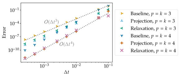
Figure 3: Convergence study for eBDF methods applied to the Kepler problem (61) with final time $t=5$ and projection/relaxation methods conserving the energy. The results for methods conserving the angular momentum are very similar.

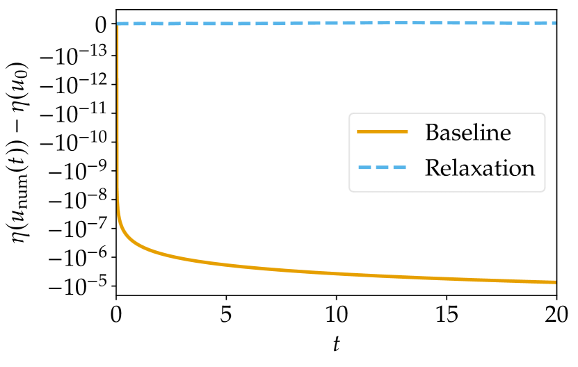
(a) Nonlinear oscillator (60), $\Delta t=0.01$.

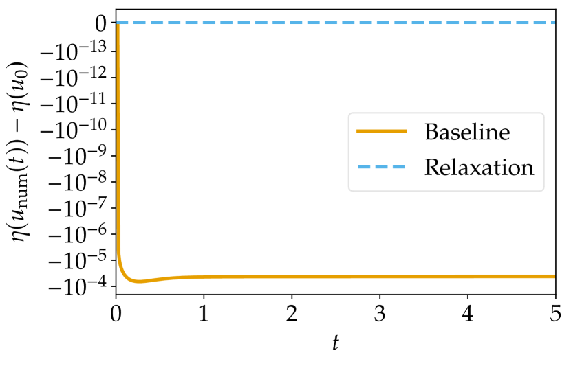
(b) Kepler problem (61), $\Delta t=0.01$.

Figure 4: Energy evolution of Adams(3) methods with and without relaxation (adapted time step and coefficients) for representative examples from Section 6.1 and 6.2.

6.3 Dissipated Exponential Entropy

Consider the ODE

$$\dfrac{\operatorname{d\!}{}}{\operatorname{d\!}{t}}u(t)=-\exp(u(t)),\quad u^{0}=0.5,$$ (65)

with exponential entropy $\eta(u)=\exp(u)$, which is dissipated for the analytical solution

$$u(t)=-\log\bigl{(}\mathrm{e}^{-1/2}+t\bigr{)}.$$ (66)

In contrast to the conservative problems described above, this problem is dissipative. We choose this test problem to demonstrate the convergence properties of relaxation methods also in this setting. Since the test problem is still not stiff, we choose a variety of explicit methods.

Again, the explicit multistep methods described above with or without projection/relaxation converge with the expected order of accuracy for this problem. As examples, third- and fourth-order accurate multistep methods yield the convergence results shown in Figure 5. There is no significant difference between the two different estimates (39) and (40) for SSP($4,3$).

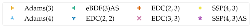
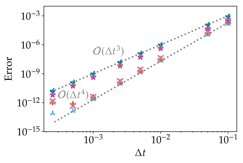
(a) Baseline methods.

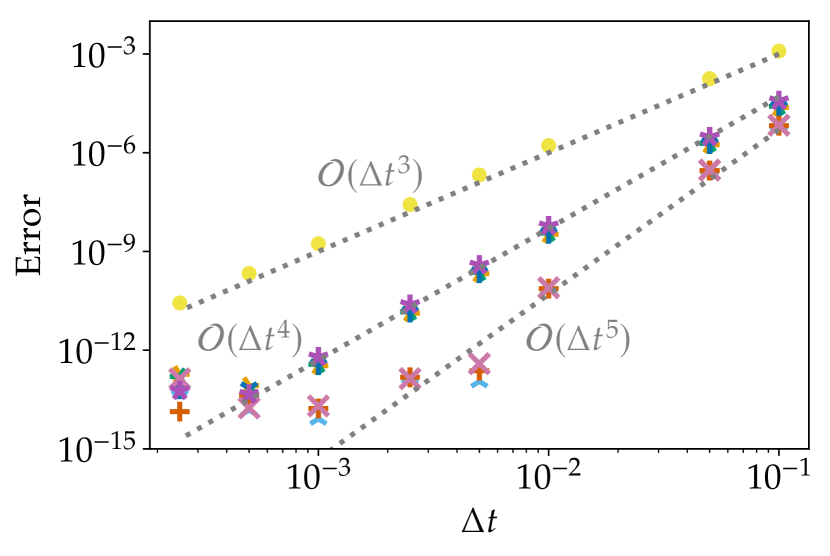
(b) Projection methods.

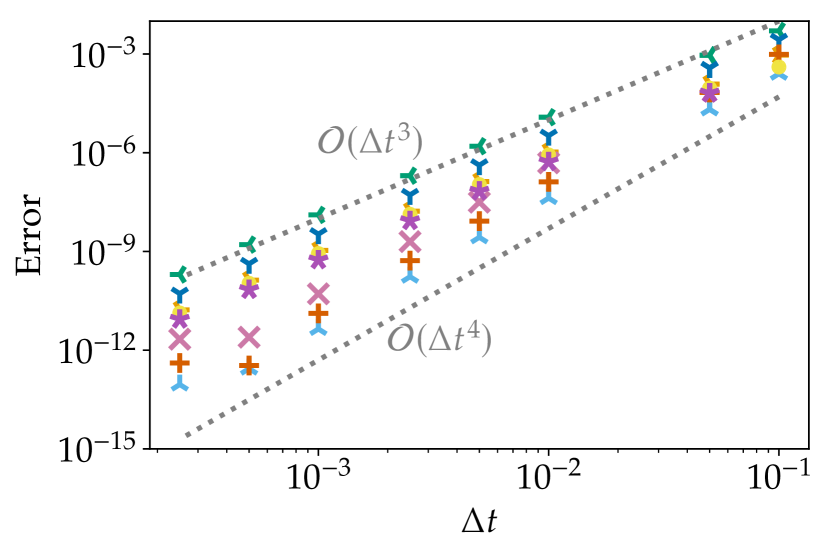
(c) Relaxation methods.

Figure 5: Convergence study for linear multistep methods applied to the ODE (65) with dissipated exponential entropy, final time $t=20$, and projection/relaxation methods based on the exponential entropy.

Results of fixed step size SSP LMMs with $\nu_{i}=\alpha_{i}$ applied to the ODE (65) with dissipated exponential entropy are shown in Figure 6. Because of the exact starting procedure, $t=\tau$ for the first $k$ steps of a $k$-step method. Thereafter, $|t-\tau|$ increases in time. As discussed in Section 4, $\max_{\tau}|t-\tau|=\mathcal{O}(\Delta\tau^{p-2})$. This can also be observed for SSP($3,2$), where the final value of $t-\tau$ is independent of the time step, and SSP($4,3$), where the final value of $t-\tau$ decreases proportionally to $\Delta\tau$. Since $\max_{\tau}|t-\tau|=\mathcal{O}(1)$ for SSP($3,2$), the maximal effective relaxation parameter $\Gamma(\tau)\gamma(\tau)$ is also $\mathcal{O}(1)$.

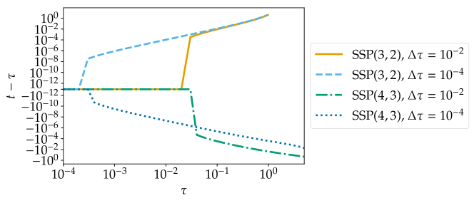
Figure 6: Difference of the physical time $t$ and the pseudotime $\tau$ for relaxation SSP LMMs with fixed step size $\Delta\tau$ applied to the ODE (65) with dissipated exponential entropy and final time $t=5$.

If $\nu_{i}\neq\alpha_{i}$, e.g. if $m=1$ and $\nu_{i}=\delta_{i,0}$ as usual for methods with adapted step sizes, no solution $\gamma>0$ can be found for this problem and the SSP LMMs with fixed step sizes. The Adams($2$) method with fixed step sizes applied to this problem works well if the final time is reduced to $t=2.5$. For larger final times, the error of the numerical solutions grows because of the growth of $\Gamma(\tau)$. Then, the time step $\Delta\tau$ has to be reduced to get acceptable solutions. The Adams methods with adapted step sizes can be applied successfully to this problem with much larger values of the time step $\Delta t$, in accordance with the analysis of Section 4.

6.4 Korteweg–de Vries Equation

The Korteweg–de Vries (KdV) equation

$$\partial_{t}u(t,x)+\partial_{x}\frac{u(t,x)^{2}}{2}+\partial_{x}^{3}u(t,x)=0$$ (67)

is well-known in the literature as a nonlinear PDE which admits soliton solutions of the form

$$u(t,x)=A\cosh\bigl{(}\sqrt{3A}(x-ct-\mu)/6\bigr{)}^{-2},\quad c=\nicefrac{{A}}{{3}},$$ (68)

where $A\geq 0$ is the amplitude, $c$ the wave speed, and $\mu$ an arbitrary constant. The KdV equation possesses an infinite hierarchy of conserved integral functionals, including the mass (with density $u$) and the energy (with density $u^{2}$).

Numerical methods that conserve both the mass and the energy result in an asymptotic error growth that is only linear in time, while other methods will in general yield an asymptotically quadratic error growth [14]. If only the energy is conserved, the error is usually reduced at first and the quadratic error growth can be seen later than for methods that do not conserve the energy.

We choose this test problem because it is a stiff nonlinear problem. Hence, we use implicit methods to deal with the stiffness. In addition, this problem demonstrates improved qualitative properties of conservative schemes and the importance of preserving linear invariants. Moreover, this stiff problem demonstrates that important stability properties are not lost by introducing relaxation, even for robust, $A$-stable methods.

Here, we use the mass- and energy-conservative Fourier collocation semidiscretization described in [52] with $N=64$ modes in an interval of length $L=80$ for the amplitude $A=2$. Integrating the resulting stiff ODE in time with the BDF($2$) method and a time step $\Delta t=0.1$ yields the results shown in Figure 7. The error for both the projection and the relaxation grows linearly in time at first. For the projection method not conserving the total mass, the error starts to grow quadratically shortly before it saturates (since there is no overlap of the numerical solution and the analytical solution anymore).

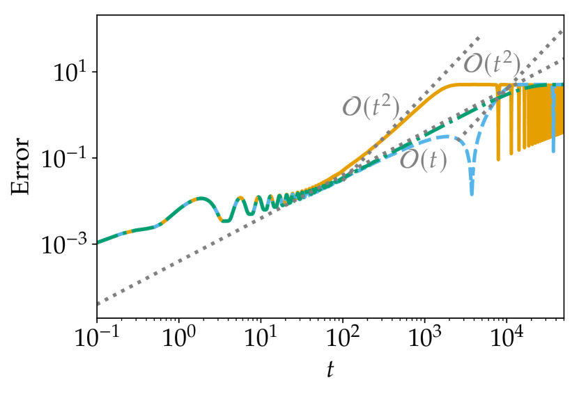
(a) Error growth in time.

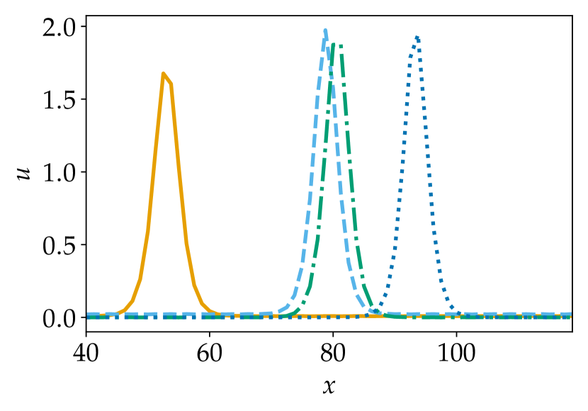
(b) Numerical solutions at the final time.

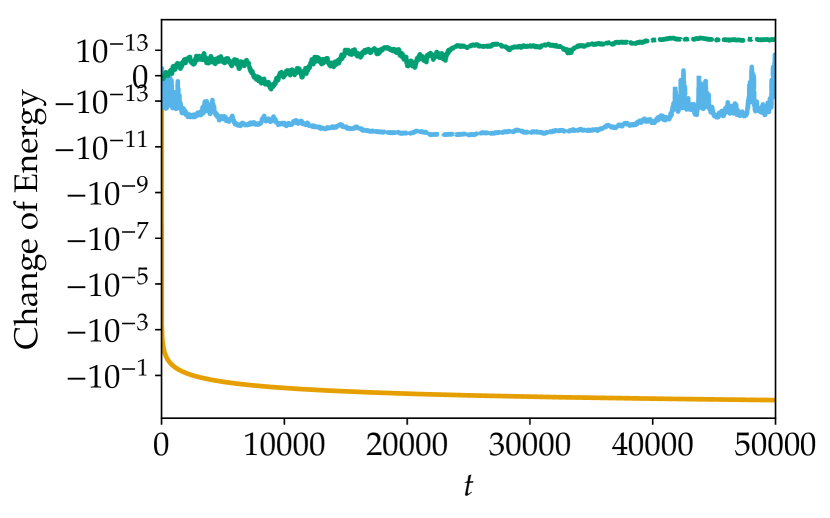
(c) Change of the total energy.

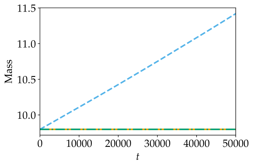
(d) Change of the total mass.

Figure 7: Numerical solutions of the KdV equation (67) with final time $t=$5.0\text{\times}{10}^{4}$$ and projection/relaxation methods conserving the energy applied to a mass- and energy-conservative Fourier collocation method. The baseline method is BDF2.

We would like to point out that we considered a long-time integration for this stiff nonlinear PDE example. The (phase) error grows in time and will reach $100\text{\,}\mathrm{\char 37\relax}$ for every time step at some time (which increases for decreasing step size $\Delta t$). In particular, having an error of $100\text{\,}\mathrm{\char 37\relax}$ after more than 400 periods of the traveling wave solution does not indicate instabilities caused choosing the time step $\Delta t$ too big. Instead, this behavior is expected and occurs also for smaller time steps (possibly after more periods).

6.5 Compressible Euler Equations

Here, we apply a second-order entropy-conservative finite difference method [68] using the entropy-conservative numerical flux of [45, Theorem 7.8] for the compressible Euler equations of an ideal gas in one space dimension. The initial condition

$$\varrho_{0}(x)=1+\frac{1}{2}\sin(\pi x),\quad v_{0}(x)=1,\quad p_{0}(x)=1,$$ (69)

where $\varrho$ is the density, $v$ the velocity, and $p$ the pressure, results in a smooth and entropy-conservative solution in the periodic domain $[0,2]$. Integrating the entropy-conservative semidiscretization with $N=100$ grid nodes in time with SSP($4,3$), where the starting values have been obtained with the relaxation version of the classical third-order, three-stage SSP Runge–Kutta method, yields the results shown in Figure 8. Clearly, the baseline scheme is not entropy-conservative while the projection method does not conserve the total mass. In contrast, the relaxation method conserves both functionals.

We choose this test problem because it is a non-stiff nonlinear PDE problem where the preservation of linear invariants is particularly interesting. We choose SSP methods since these are often applied to computational fluid dynamics; results for other time integration methods are similar since the SSP property is not crucial here.

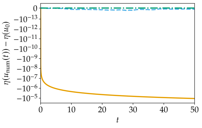
(a) Total entropy change.

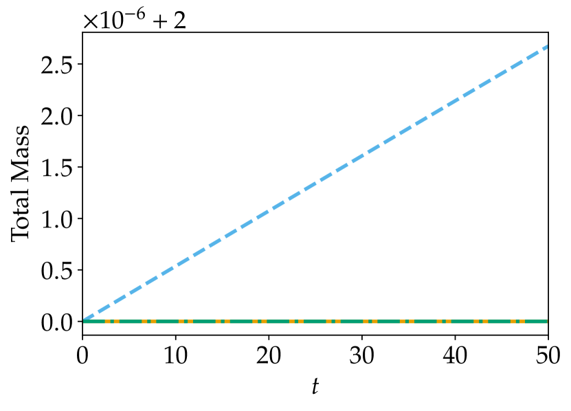
(b) Total mass.

Figure 8: Numerical solutions of the compressible Euler equations with final time $t=50$ and time step $\Delta t=0.1\Delta x$ using entropy-conservative finite differences and projection/relaxation versions of SSP($4,3$).

6.6 Burgers’ Equation

Solutions of Burgers’ equation

$$\partial_{t}u(t,x)+\partial_{x}\frac{u(t,x)^{2}}{2}=0,\quad u(0,x)=\exp(-30x^{2}),$$ (70)

in the periodic domain $[-1,1]$ develop shocks in a finite time. Hence, energy-conservative methods are not appropriate. Here, we apply the same energy-dissipative semidiscretization used in [32] in the context of relaxation Runge–Kutta methods, which can be written as

$$\dfrac{\operatorname{d\!}{}}{\operatorname{d\!}{t}}u_{i}(t)=-\frac{f^{\mathrm{num}}(u_{i},u_{i+1})-f^{\mathrm{num}}(u_{i-1},u_{i})}{\Delta x}.$$ (71)

The energy-dissipative numerical flux is obtained by adding some dissipation to the energy-conservative flux, resulting in

$$f^{\mathrm{num}}(u_{-},u_{+})=\frac{u_{-}^{2}+u_{-}u_{+}+u_{+}^{2}}{6}-\varepsilon(u_{+}-u_{-}).$$ (72)

These semidiscretizations are integrated in time with SSP($3,2$) and SSP($4,3$), where the starting values have been obtained with the relaxation version of the classical third order, three-stage SSP Runge–Kutta method.

We choose this test problem because it is a non-stiff nonlinear PDE problem with decaying energy to demonstrate improved qualitative behavior also in this context. We choose SSP methods again since these are often applied to computational fluid dynamics problems.

The changes of the total energy and mass of the numerical solutions and a semidiscrete reference solution are visualized in Figure 9. The baseline schemes are either anti-dissipative (for SSPRK($3,2$)) or too dissipative (for SSPRK($4,3$)) compared to the reference solution, similarly to results for Runge–Kutta methods shown in [32]. In contrast, the energy dissipation of both the relaxation and the projection versions agrees very well with the reference solution. However, the projection schemes change the total mass while the relaxation methods conserve this invariant of the PDE (70).

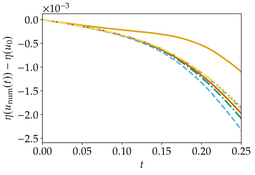
(a) Total energy change.

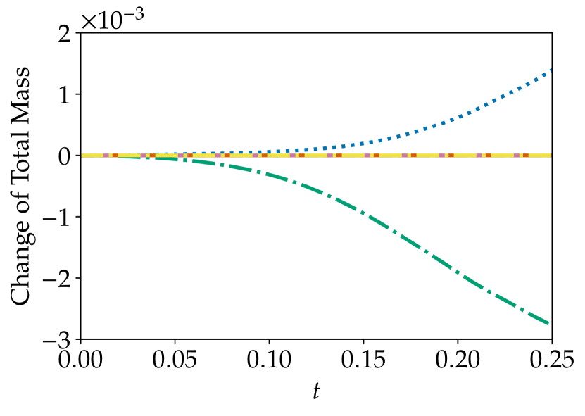
(b) Total mass change.

Figure 9: Numerical solutions of Burgers’ equation with final time $t=0.25$ and time step $\Delta t=0.2\Delta x$ using energy-dissipative finite differences and projection/relaxation versions of SSP($3,2$) and SSP($4,3$).

Adding instead some dissipation to a semidiscretization based on the central numerical flux

$$f^{\mathrm{num}}(u_{-},u_{+})=\frac{u_{-}^{2}+u_{+}^{2}}{4}-\varepsilon(u_{+}-u_{-})$$ (73)

does not yield a provably energy-dissipative semidiscretization in general. However, the relaxation methods still improve the energy evolution as visualized in Figure 10.

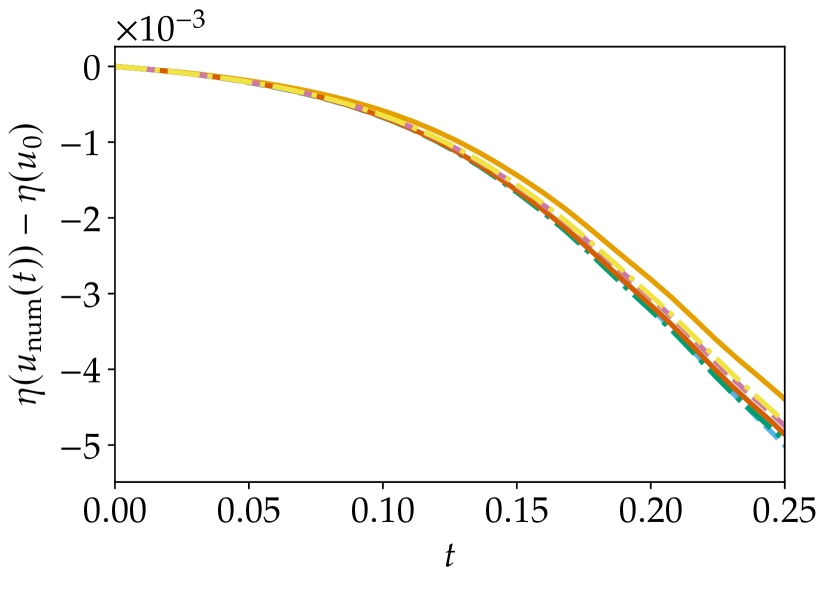
(a) Total energy change.

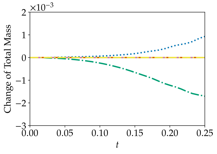
(b) Total mass change.

Figure 10: Numerical solutions of Burgers’ equation with final time $t=0.25$ and time step $\Delta t=0.2\Delta x$ using central finite differences with dissipation and projection/relaxation versions of SSP($3,2$) and SSP($4,3$).

6.7 Linear Advection with Inflow

Solutions of the linear advection equation

$$\partial_{t}u(t,x)+\partial_{x}u(t,x) =0, t\in(0,6),\,x\in(0,3),$$ (74)

$$u(0,x) =0, x\in[0,3],$$

$$u(t,0) =\sin(\pi t), t\in[0,6],$$

do neither conserve nor dissipate the energy $\frac{1}{2}\mathinner{\!\left\lVert u\right\rVert}_{L^{2}}^{2}$ because of the boundary condition. Instead, the energy of the analytical solution increases till $t=3$ to its final value $0.75$ and stays constant thereafter. We choose this test problem because it results in a non-monotone behavior of the energy. We choose SSP methods again since these are often applied to computational fluid dynamics problems.

Using the classical second-order summation-by-parts operator with simultaneous approximation terms to impose the boundary condition weakly [67] on $N=200$ uniformly spaced nodes yields an ODE with a similar behavior. As visualized in Figure 11, the baseline SSP($3,2$) method results in an increase of the energy that is slightly bigger than that of the reference solution obtained by SSP($4,3$) with much smaller time steps. Instead, the energy variation enforced by the projection and relaxation methods is visually indistinguishable from the reference value. The slight variations of the energy for $t>3$ are caused by the spatial semidiscretizations using a weak imposition of the boundary condition.

This example demonstrates that relaxation methods can also be useful for non-dissipative systems where energy or entropy estimates can still be obtained and are of interest. In [54], a similar lid-driven cavity flow with a heated wall for the Navier–Stokes equations has been solved with relaxation Runge–Kutta methods.

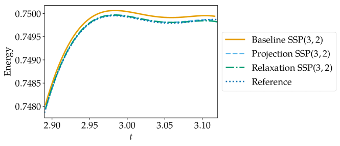
Figure 11: Energy of numerical solutions of the linear advection equation (74) computed with or without projection/relaxation methods and SSP(3, 2).

6.8 Some Remarks on the Costs of Relaxation

For a quadratic or cubic entropy functional, the relaxation parameter can be computed explicitly. For more general entropies, it must be found via numerical iteration.

We have used SciPy [70] to solve the scalar equations for the relaxation parameter $\gamma^{n}$. Our implementations are based on functions written in pure Python and are not adapted to the specific problems. A detailed assessment of the computational cost of solving for the relaxation parameter $\gamma^{n}$ requires a more refined implementation and is beyond the scope of this work. Nevertheless, we give some preliminary discussion of the costs here, emphasizing that these numbers should be viewed as very crude upper bounds on the cost associated to relaxation.

For explicit time-stepping methods and very inexpensive right-hand sides, the costs of naive implementations of the relaxation approach are significant. For the example of the compressible Euler equations in Section 6.5, relaxation methods increase the runtime by a factor between two and three. For Burgers’ equation as in Section 6.6, the total runtime increases by less than a factor of two. Although the relaxation technique increases the runtime significantly in this naive implementation, it is still cheaper than decreasing the time step to get basically the same results.

Relaxation methods were applied to large-scale PDE discretizations of the compressible Euler and Navier-Stokes equations in three space dimensions in [54, 48]. In that context, the cost associated with solving the single scalar equation for the relaxation parameter $\gamma^{n}$ is much less than the cost of evaluating the right-hand side of the ODE during one time step.

When implicit time-stepping is used, the cost of relaxation is less significant. This was already discussed in [52] for the KdV equation. There, the energy-conserving methods decreased the runtime despite the added overhead of computing the relaxation or projection step. The reason for this is the improved accuracy and hence decreased costs to solve the nonlinear stage equations. The relaxation method benefited additionally from taking larger effective time steps since the relaxation parameter $\gamma^{n}>1$.

7 Summary and Conclusions

We have extended the framework of relaxation methods for the numerical solution of initial-value problems from Runge–Kutta methods to general time integration schemes with order of accuracy $p\geq 2$. By solving a single scalar algebraic equation per time step, the evolution in time of a given functional can be preserved. This includes functionals that are conserved or dissipated, as well as others for which estimates of the time evolution are available. For convex functionals, additional insights such as the possibility to add dissipation in time have been provided.

For certain classes of relaxation linear multistep methods, high-order accuracy is still attained even if a fixed-coefficient method is used. Nevertheless, we recommend the use of methods that correctly account for the step size variation, since such methods gave overall better results in numerical tests.

In contrast to orthogonal projection methods, relaxation methods preserve all linear invariants that are preserved by the baseline time integration scheme (which are all linear invariants of the ODE for general linear methods). This property can be very important, e.g. for conservation laws.

We have also studied the impact of the relaxation approach on other stability properties of time integration methods. In particular, zero stability and strong stability preserving properties of linear multistep and Runge–Kutta methods are not changed significantly.

While relaxation methods appear to provide good results in our numerical experiments, further practical experience on a wide range of problems is still needed to determine their general effectiveness. Other areas of ongoing research include the development of other means to estimate the change of a dissipated functional $\eta$ and development of a spatially localized relaxation approach for conservation laws with convex entropies.

Appendix A Superconvergence for Euclidean Hamiltonian Problems

Here, we present a generalization of the superconvergence Theorem 4.1 of [52] to general energy-conservative B-series [27] time integration methods, see e.g. [39] and the references cited therein. This general class of time integration schemes includes among others Runge–Kutta methods, linear multistep methods, Taylor series methods, and Rosenbrock methods.

Consider a Hamiltonian $H$ that is a smooth function of the squared Euclidean norm, i.e.

$$H(q,p)=G\bigl{(}(|q|^{2}+|p|^{2})/2\bigr{)},$$ (75)

where $G$ is a smooth function. The corresponding Hamiltonian system is

$$\begin{cases}u^{\prime}(t)=f(u(t)),\\ u(0)=u^{0},\end{cases}\quad u(t)=\begin{pmatrix}q(t)\\ p(t)\end{pmatrix},\quad f(q,p)=g\bigl{(}(|q|^{2}+|p|^{2})/2\bigr{)}\begin{pmatrix}p\\ -q\end{pmatrix},$$ (76)

where $g=G^{\prime}$. We refer to (76) as a Euclidean Hamiltonian problem. For this class of problems, nominally odd-order energy-conservative B-series time integration methods are superconvergent.

The proof relies on a special geometric structure of the error. As shown in [52, Lemma A.4], for (76) the local error can be divided into two parts. The part that is along the manifold of constant $H$ includes all terms with even powers of $\Delta t$, while the part orthogonal to the manifold of constant $H$ includes all terms with odd powers of $\Delta t$. Thus a solution that preserves $H$ has no error terms with odd powers of $\Delta t$.

Theorem A.1.

Consider the general nonlinear Euclidean Hamiltonian system (76) with $g\neq 0$ and a B-series time integration method of order $p$ with or without applying orthogonal projection or relaxation.

If the method conserves the Hamiltonian, the expansion of the local error contains only odd powers of $\Delta t$. In particular, its order of accuracy for the system (76) is $p+1$ if $p$ is odd.

Proof.

It suffices to consider the local error after one step, which can be written as

$$u^{n}-u(t^{n-1}+\Delta t)=\sum_{k=p+1}^{\infty}\Delta t^{k}\sum_{\mathinner{\!\left\lvert t\right\rvert}=k}e_{t}F(t)(u^{n-1}),$$ (77)

where $e_{t}$ are some coefficients of the local error, the second sum is a sum over all rooted trees $t$ of order $k$, cf. [8, Chapter 3], and $F(t)(u^{n-1})$ is an elementary differential of $f$ evaluated at $u^{n-1}$.

Since the method is energy-conservative, it conserves the Euclidean norm. Hence, for any $k\geq p+1$,

$$0 =\frac{\mathrm{d}^{k}}{\operatorname{d\!}\Delta t^{k}}\bigg{|}_{\Delta t=0}\left(\|u^{n}\|^{2}-\|u(t^{n-1}+\Delta t)\|^{2}\right)$$ (78)

$$=\frac{\mathrm{d}^{k}}{\operatorname{d\!}\Delta t^{k}}\bigg{|}_{\Delta t=0}\left\langle{u^{n}-u(t^{n-1}+\Delta t),\,u^{n}+u(t^{n-1}+\Delta t)}\right\rangle$$

$$=\left\langle{\frac{\mathrm{d}^{k}}{\operatorname{d\!}\Delta t^{k}}\bigg{|}_{\Delta t=0}\left(u^{n}-u(t^{n-1}+\Delta t)\right),\,2u^{n-1}}\right\rangle$$

$$=2k\sum_{\mathinner{\!\left\lvert t\right\rvert}=k}e_{t}\left\langle{F(t)(u^{n-1}),\,u^{n-1}}\right\rangle.$$

For even $k$, $F(t)(u^{n-1})\parallel u^{n-1}$ for $\mathinner{\!\left\lvert t\right\rvert}=k$ because of [52, Lemma A.4]. Hence, $\sum_{\mathinner{\!\left\lvert t\right\rvert}=k}e_{t}F(t)(u^{n-1})=0$ for even $k$. ∎

Appendix B An Example for Which Relaxation LMMs are Exact

Here we consider a problem from [54]:

$$u_{1}^{\prime}(t) =-\exp(u_{2}),$$ (79a)

$$u_{2}^{\prime}(t) =\exp(u_{1}).$$ (79b)

The entropy $\eta(u)=\exp(u_{1})+\exp(u_{2})$ is conserved. The exact solution is given by

$$u_{1}(t) =\log\left(\frac{C\eta}{C+e^{\eta t}}\right), u_{2}(t) =\log\left(\frac{\eta e^{\eta t}}{C+e^{\eta t}}\right),$$ (80)

where $\eta=\exp(u_{1})+\exp(u_{2})$ and $C=e^{u_{1}(0)-u_{2}(0)}.$

Theorem B.1.

Let a relaxation LMM of order two or greater be applied to (79), with $\Delta t$ small enough such that there exists a value of $\gamma$ satisfying (8). If the starting values are exact, then the numerical solution is (in the absence of rounding errors) exact at each step.

Proof.

First observe that the equations

$$w=u_{2}-u_{1},\qquad\eta=\exp(u_{1})+\exp(u_{2}),$$ (81)

define a bijection between $(u_{1},u_{2})\in\mathbb{R}^{2}$ and $(w,\eta)\in\mathbb{R}\times\mathbb{R}^{+}$. Thus (79) is equivalent to the system

$$w^{\prime}(t) =\eta,$$ (82a)

$$\eta^{\prime}(t) =0,$$ (82b)

with the solution $w(t)=\eta(0)t+w(0)$ and $\eta(t)=\eta(0)$. We will show that any relaxation LMM integrates the system (82) exactly. We can write any LMM as

$$u^{\mathrm{new}}=\sum_{j=0}^{k-1}\alpha_{j}u^{n-k+j}+\Delta t\sum_{j=0}^{k}\beta_{j}f(u^{n-k+j}).$$ (83)

Taking the difference of the formulas for $u^{n}_{2}$ and $u^{n}_{1}$ we obtain

$$w^{n}=\sum_{j=0}^{k-1}\alpha_{j}w^{n-k+j}+\Delta t\eta\sum_{j=0}^{k}\beta_{j}.$$ (84)

Since the starting values are exact, $w^{n-k+j}=w(t^{n-k+j})$. Due to the consistency of the LMM, this means that the formula above is exact; i.e. $w^{n}=w(t^{n-1}+\Delta t)$. Next we take

$$w^{n}_{\gamma}=w^{n-m}+\gamma(w^{n}-w^{n-m})=w(t^{n}+\gamma\Delta t),$$ (85)

since $w(t)$ is linear. Thus the numerical solution given by the relaxation LMM gives the exact value for $w$. It also gives the exact value for $\eta$, since this is precisely what is enforced by relaxation. ∎

Remark B.2.

Note that without the relaxation step, the solution is not exact since the equation for $w(t)$ is solved exactly but that for $\eta(t)$ is not. Projection methods do not solve (79) exactly, because the projection step does not preserve the exact solution of the linear ODE for $w(t)$. Relaxation Runge–Kutta methods (and other multistage methods) also do not solve (79) exactly, because they involve iterated evaluation of the nonlinear RHS within a single step, so they do not effectively integrate the linear ODE for $w(t)$ exactly.

References

- [1] Carmen Arévalo, Claus Führer and Gustaf Söderlind “Regular and singular -blocking of difference corrected multistep methods for nonstiff index-2 DAEs” In Applied Numerical Mathematics 35.4 Elsevier, 2000, pp. 293–305 DOI: 10.1016/S0168-9274(99)00142-7
- [2] Carmen Arévalo and Gustaf Söderlind “Grid-independent construction of multistep methods” In Journal of Computational Mathematics 35.5, 2017, pp. 672–692 DOI: 10.4208/jcm.1611-m2015-0404
- [3] Francis Bashforth and John Couch Adams “An attempt to test the theories of capillary action by comparing the theoretical and measured forms of drops of fluid with an explanation of the method of integration employed in constructing the tables which give the theoretical forms of such drops” Cambridge: Cambridge University Press, 1883
- [4] Pieter D Boom and David W Zingg “High-order implicit time-marching methods based on generalized summation-by-parts operators” In SIAM Journal on Scientific Computing 37.6 SIAM, 2015, pp. A2682–A2709 DOI: 10.1137/15M1014917
- [5] Hans Burchard, Eric Deleersnijder and Andreas Meister “A high-order conservative Patankar-type discretisation for stiff systems of production–destruction equations” In Applied Numerical Mathematics 47.1 Elsevier, 2003, pp. 1–30 DOI: 10.1016/S0168-9274(03)00101-6
- [6] Kevin Burrage and John Charles Butcher “Non-linear stability of a general class of differential equation methods” In BIT Numerical Mathematics 20.2 Springer, 1980, pp. 185–203 DOI: 10.1007/BF01933191
- [7] Kevin Burrage and John Charles Butcher “Stability criteria for implicit Runge–Kutta methods” In SIAM Journal on Numerical Analysis 16.1 SIAM, 1979, pp. 46–57 DOI: 10.1137/0716004
- [8] John Charles Butcher “Numerical Methods for Ordinary Differential Equations” Chichester: John Wiley & Sons Ltd, 2016 DOI: 10.1002/9781119121534
- [9] Manuel Calvo, D Hernández-Abreu, Juan I Montijano and Luis Rández “On the Preservation of Invariants by Explicit Runge–Kutta Methods” In SIAM Journal on Scientific Computing 28.3 SIAM, 2006, pp. 868–885 DOI: 10.1137/04061979X
- [10] Manuel Calvo, MP Laburta, JI Montijano and L Rández “Projection methods preserving Lyapunov functions” In BIT Numerical Mathematics 50.2 Springer, 2010, pp. 223–241 DOI: 10.1007/s10543-010-0259-3
- [11] Jesse Chan “On discretely entropy conservative and entropy stable discontinuous Galerkin methods” In Journal of Computational Physics 362 Elsevier, 2018, pp. 346–374 DOI: 10.1016/j.jcp.2018.02.033
- [12] Charles Francis Curtiss and Joseph O Hirschfelder “Integration of stiff equations” In Proceedings of the National Academy of Sciences of the United States of America 38.3 National Academy of Sciences, 1952, pp. 235 DOI: 10.1073/pnas.38.3.235
- [13] Constantine M Dafermos “Hyperbolic Conservation Laws in Continuum Physics” Berlin Heidelberg: Springer-Verlag, 2010 DOI: 10.1007/978-3-642-04048-1
- [14] J De Frutos and Jesus Maria Sanz-Serna “Accuracy and conservation properties in numerical integration: the case of the Korteweg-de Vries equation” In Numerische Mathematik 75.4 Springer, 1997, pp. 421–445 DOI: 10.1007/s002110050247
- [15] Kees Dekker and Jan G Verwer “Stability of Runge–Kutta methods for stiff nonlinear differential equations” 2, CWI Monographs Amsterdam: North-Holland, 1984
- [16] Edda Eich “Convergence results for a coordinate projection method applied to mechanical systems with algebraic constraints” In SIAM Journal on Numerical Analysis 30.5 SIAM, 1993, pp. 1467–1482 DOI: 10.1137/0730076
- [17] Travis C Fisher and Mark H Carpenter “High-order entropy stable finite difference schemes for nonlinear conservation laws: Finite domains” In Journal of Computational Physics 252 Elsevier, 2013, pp. 518–557 DOI: 10.1016/j.jcp.2013.06.014
- [18] Lucas Friedrich et al. “Entropy Stable Space–Time Discontinuous Galerkin Schemes with Summation-by-Parts Property for Hyperbolic Conservation Laws” In Journal of Scientific Computing 80.1 Springer, 2019, pp. 175–222 DOI: 10.1007/s10915-019-00933-2
- [19] Lucas Friedrich et al. “An entropy stable h/p non-conforming discontinuous Galerkin method with the summation-by-parts property” In Journal of Scientific Computing 77.2 Springer, 2018, pp. 689–725 DOI: 10.1007/s10915-018-0733-7
- [20] Charles William Gear “Maintaining solution invariants in the numerical solution of ODEs” In SIAM Journal on Scientific and Statistical Computing 7.3 SIAM, 1986, pp. 734–743 DOI: 10.1137/0907050
- [21] Jan Glaubitz, Philipp Öffner, Hendrik Ranocha and Thomas Sonar “Artificial Viscosity for Correction Procedure via Reconstruction Using Summation-by-Parts Operators” In Theory, Numerics and Applications of Hyperbolic Problems II 237, Springer Proceedings in Mathematics & Statistics Cham: Springer International Publishing, 2018, pp. 363–375 DOI: 10.1007/978-3-319-91548-7_28
- [22] Sigal Gottlieb, David I Ketcheson and Chi-Wang Shu “Strong stability preserving Runge–Kutta and multistep time discretizations” Singapore: World Scientific, 2011
- [23] V Grimm and GRW Quispel “Geometric integration methods that preserve Lyapunov functions” In BIT Numerical Mathematics 45.4 Springer, 2005, pp. 709–723 DOI: 10.1007/s10543-005-0034-z
- [24] Yiannis Hadjimichael, David I Ketcheson, Lajos Lóczi and Adrián Németh “Strong stability preserving explicit linear multistep methods with variable step size” In SIAM Journal on Numerical Analysis 54.5 SIAM, 2016, pp. 2799–2832 DOI: 10.1137/15M101717X
- [25] Ernst Hairer, Christian Lubich and Gerhard Wanner “Geometric Numerical Integration: Structure-Preserving Algorithms for Ordinary Differential Equations” 31, Springer Series in Computational Mathematics Berlin Heidelberg: Springer-Verlag, 2006 DOI: 10.1007/3-540-30666-8
- [26] Ernst Hairer, Syvert Paul Nørsett and Gerhard Wanner “Solving Ordinary Differential Equations I: Nonstiff Problems” 8, Springer Series in Computational Mathematics Berlin Heidelberg: Springer-Verlag, 2008 DOI: 10.1007/978-3-540-78862-1
- [27] Ernst Hairer and Gerhard Wanner “On the Butcher group and general multi-value methods” In Computing 13.1 Springer, 1974, pp. 1–15 DOI: 10.1007/BF02268387
- [28] Ernst Hairer and Gerhard Wanner “Solving Ordinary Differential Equations II: Stiff and Differential-Algebraic Problems” 14, Springer Series in Computational Mathematics Berlin Heidelberg: Springer-Verlag, 2010 DOI: 10.1007/978-3-642-05221-7
- [29] Inmaculada Higueras “Monotonicity for Runge–Kutta Methods: Inner Product Norms” In Journal of Scientific Computing 24.1 Springer, 2005, pp. 97–117 DOI: 10.1007/s10915-004-4789-1
- [30] J. D. Hunter “Matplotlib: A 2D graphics environment” In Computing in Science & Engineering 9.3 IEEE Computer Society, 2007, pp. 90–95 DOI: 10.1109/MCSE.2007.55
- [31] Ansgar Jüngel and Stefan Schuchnigg “Entropy-dissipating semi-discrete Runge–Kutta schemes for nonlinear diffusion equations” In Communications in Mathematical Sciences 15.1 International Press of Boston, 2017, pp. 27–53 DOI: 10.4310/CMS.2017.v15.n1.a2
- [32] David I Ketcheson “Relaxation Runge–Kutta Methods: Conservation and Stability for Inner-Product Norms” In SIAM Journal on Numerical Analysis 57.6 Society for IndustrialApplied Mathematics, 2019, pp. 2850–2870 DOI: 10.1137/19M1263662
- [33] Hiroki Kojima “Invariants preserving schemes based on explicit Runge–Kutta methods” In BIT Numerical Mathematics 56.4 Springer, 2016, pp. 1317–1337 DOI: 10.1007/s10543-016-0608-y
- [34] MP Laburta, Juan I Montijano, Luis Rández and Manuel Calvo “Numerical methods for non conservative perturbations of conservative problems” In Computer Physics Communications 187 Elsevier, 2015, pp. 72–82 DOI: 10.1016/j.cpc.2014.10.012
- [35] Philippe G LeFloch, Jean-Marc Mercier and Christian Rohde “Fully Discrete, Entropy Conservative Schemes of Arbitrary Order” In SIAM Journal on Numerical Analysis 40.5 Society for IndustrialApplied Mathematics, 2002, pp. 1968–1992 DOI: 10.1137/S003614290240069X
- [36] Randall J. LeVeque “Finite Difference Methods for Ordinary and Partial Differential Equations: steady-state and time-dependent problems” SIAM, 2007
- [37] Carlos Lozano “Entropy Production by Explicit Runge–Kutta Schemes” In Journal of Scientific Computing 76.1 Springer, 2018, pp. 521–565 DOI: 10.1007/s10915-017-0627-0
- [38] Carlos Lozano “Entropy Production by Implicit Runge–Kutta Schemes” In Journal of Scientific Computing Springer, 2019 DOI: 10.1007/s10915-019-00914-5
- [39] Robert I McLachlan, Klas Modin, Hans Munthe-Kaas and Olivier Verdier “B-series methods are exactly the affine equivariant methods” In Numerische Mathematik 133.3 Springer, 2016, pp. 599–622 DOI: 10.1007/s00211-015-0753-2
- [40] Fatemeh Mohammadi, Carmen Arévalo and Claus Führer “A polynomial formulation of adaptive strong stability preserving multistep methods” In SIAM Journal on Numerical Analysis 57.1 SIAM, 2019, pp. 27–43 DOI: 10.1137/17M1158811
- [41] Jan Nordström and Cristina La Cognata “Energy stable boundary conditions for the nonlinear incompressible Navier–Stokes equations” In Mathematics of Computation 88.316 American Mathematical Society, 2019, pp. 665–690 DOI: 10.1090/mcom/3375
- [42] Evert Johannes Nyström “Über die numerische Integration von Differentialgleichungen” In Acta Societatis Scientiarum Fennicae 50.13 Societas Scientiarum Fennica, 1925, pp. 1–56
- [43] Philipp Öffner, Jan Glaubitz and Hendrik Ranocha “Analysis of Artificial Dissipation of Explicit and Implicit Time-Integration Methods” In International Journal of Numerical Analysis and Modeling 17.3 Global Science Press, 2020, pp. 332–349 arXiv:1609.02393 [math.NA]
- [44] Hendrik Ranocha “Comparison of Some Entropy Conservative Numerical Fluxes for the Euler Equations” In Journal of Scientific Computing 76.1 Springer, 2018, pp. 216–242 DOI: 10.1007/s10915-017-0618-1
- [45] Hendrik Ranocha “Generalised Summation-by-Parts Operators and Entropy Stability of Numerical Methods for Hyperbolic Balance Laws”, 2018
- [46] Hendrik Ranocha “On Strong Stability of Explicit Runge-Kutta Methods for Nonlinear Semibounded Operators” In IMA Journal of Numerical Analysis Oxford University Press, 2020 DOI: 10.1093/imanum/drz070
- [47] Hendrik Ranocha “Some Notes on Summation by Parts Time Integration Methods” In Results in Applied Mathematics 1 Elsevier, 2019, pp. 100004 DOI: 10.1016/j.rinam.2019.100004
- [48] Hendrik Ranocha, Lisandro Dalcin and Matteo Parsani “Fully-Discrete Explicit Locally Entropy-Stable Schemes for the Compressible Euler and Navier-Stokes Equations” In Computers and Mathematics with Applications 80.5 Elsevier, 2020, pp. 1343–1359 DOI: 10.1016/j.camwa.2020.06.016
- [49] Hendrik Ranocha, Jan Glaubitz, Philipp Öffner and Thomas Sonar “Stability of artificial dissipation and modal filtering for flux reconstruction schemes using summation-by-parts operators” See also arXiv: 1606.00995 [math.NA] and arXiv: 1606.01056 [math.NA] In Applied Numerical Mathematics 128 Elsevier, 2018, pp. 1–23 DOI: 10.1016/j.apnum.2018.01.019
- [50] Hendrik Ranocha and David I Ketcheson “Energy Stability of Explicit Runge-Kutta Methods for Non-autonomous or Nonlinear Problems” Accepted in SIAM Journal on Numerical Analysis, 2020 arXiv:1909.13215 [math.NA]
- [51] Hendrik Ranocha and David I Ketcheson “Relaxation-LMM-notebooks. General Relaxation Methods for Initial-Value Problems with Application to Multistep Schemes”, https://github.com/ranocha/Relaxation-LMM-notebooks, 2020 DOI: 10.5281/zenodo.3697836
- [52] Hendrik Ranocha and David I Ketcheson “Relaxation Runge-Kutta Methods for Hamiltonian Problems” In Journal of Scientific Computing 84.1 Springer Nature, 2020 DOI: 10.1007/s10915-020-01277-y
- [53] Hendrik Ranocha and Philipp Öffner “ Stability of Explicit Runge–Kutta Schemes” In Journal of Scientific Computing 75.2, 2018, pp. 1040–1056 DOI: 10.1007/s10915-017-0595-4
- [54] Hendrik Ranocha et al. “Relaxation Runge–Kutta Methods: Fully-Discrete Explicit Entropy-Stable Schemes for the Compressible Euler and Navier–Stokes Equations” In SIAM Journal on Scientific Computing 42.2 Society for IndustrialApplied Mathematics, 2020, pp. A612–A638 DOI: 10.1137/19M1263480
- [55] Maxwell Rosenlicht “Introduction to Analysis” New York: Dover Publications, Inc., 1986
- [56] Steven J Ruuth and Willem Hundsdorfer “High-order linear multistep methods with general monotonicity and boundedness properties” In Journal of Computational Physics 209.1 Elsevier, 2005, pp. 226–248 DOI: 10.1016/j.jcp.2005.02.029
- [57] Jesus Maria Sanz-Serna “An explicit finite-difference scheme with exact conservation properties” In Journal of Computational Physics 47.2 Elsevier, 1982, pp. 199–210 DOI: 10.1016/0021-9991(82)90074-2
- [58] Jesus Maria Sanz-Serna and Manuel P Calvo “Numerical Hamiltonian Problems” 7, Applied Mathematics and Mathematical Computation London: Chapman & Hall, 1994
- [59] Jesus Maria Sanz-Serna and VS Manoranjan “A method for the integration in time of certain partial differential equations” In Journal of Computational Physics 52.2 Elsevier, 1983, pp. 273–289 DOI: 10.1016/0021-9991(83)90031-1
- [60] Lawrence F Shampine “Conservation laws and the numerical solution of ODEs” In Computers & Mathematics with Applications 12.5-6 Pergamon, 1986, pp. 1287–1296 DOI: 10.1016/0898-1221(86)90253-1
- [61] Lawrence F Shampine “Conservation laws and the numerical solution of ODEs, II” In Computers & Mathematics with Applications 38.2 Elsevier, 1999, pp. 61–72 DOI: 10.1016/S0898-1221(99)00183-2
- [62] Björn Sjögreen and HC Yee “High order entropy conservative central schemes for wide ranges of compressible gas dynamics and MHD flows” In Journal of Computational Physics 364 Elsevier, 2018, pp. 153–185 DOI: 10.1016/j.jcp.2018.02.003
- [63] Gustaf Söderlind, Imre Fekete and István Faragó “On the zero-stability of multistep methods on smooth nonuniform grids” In BIT Numerical Mathematics 58.4 Springer, 2018, pp. 1125–1143 DOI: 10.1007/s10543-018-0716-y
- [64] Zheng Sun and Chi-Wang Shu “Enforcing strong stability of explicit Runge–Kutta methods with superviscosity”, 2019 arXiv:1912.11596 [math.NA]
- [65] Zheng Sun and Chi-Wang Shu “Stability of the fourth order Runge–Kutta method for time-dependent partial differential equations” In Annals of Mathematical Sciences and Applications 2.2, 2017, pp. 255–284 DOI: 10.4310/AMSA.2017.v2.n2.a3
- [66] Zheng Sun and Chi-Wang Shu “Strong Stability of Explicit Runge–Kutta Time Discretizations” In SIAM Journal on Numerical Analysis 57.3 SIAM, 2019, pp. 1158–1182 DOI: 10.1137/18M122892X
- [67] Magnus Svärd and Jan Nordström “Review of summation-by-parts schemes for initial-boundary-value problems” In Journal of Computational Physics 268 Elsevier, 2014, pp. 17–38 DOI: 10.1016/j.jcp.2014.02.031
- [68] Eitan Tadmor “Entropy stability theory for difference approximations of nonlinear conservation laws and related time-dependent problems” In Acta Numerica 12 Cambridge University Press, 2003, pp. 451–512 DOI: 10.1017/S0962492902000156
- [69] Eitan Tadmor “From Semidiscrete to Fully Discrete: Stability of Runge–Kutta Schemes by the Energy Method II” In Collected Lectures on the Preservation of Stability under Discretization 109, Proceedings in Applied Mathematics Philadelphia: Society for IndustrialApplied Mathematics, 2002, pp. 25–49
- [70] Pauli Virtanen et al. “SciPy 1.0 – Fundamental Algorithms for Scientific Computing in Python”, 2019 arXiv:1907.10121 [cs.MS]
- [71] Hamed Zakerzadeh and Ulrik Skre Fjordholm “High-order accurate, fully discrete entropy stable schemes for scalar conservation laws” In IMA Journal of Numerical Analysis 36.2 Oxford University Press, 2016, pp. 633–654 DOI: 10.1093/imanum/drv020