Bayesian Spatial Homogeneity Pursuit for Survival Data with an Application to the SEER Respiratory Cancer Data

Abstract

In this work, we propose a new Bayesian spatial homogeneity pursuit method for survival data under the proportional hazards model to detect spatially clustered patterns in baseline hazard and regression coefficients. Specially, regression coefficients and baseline hazard are assumed to have spatial homogeneity pattern over space. To capture such homogeneity, we develop a geographically weighted Chinese restaurant process prior to simultaneously estimate coefficients and baseline hazards and their uncertainty measures. An efficient Markov chain Monte Carlo (MCMC) algorithm is designed for our proposed methods. Performance is evaluated using simulated data, and further applied to a real data analysis of respiratory cancer in the state of Louisiana.

Keywords: Geographically Weighted Chinese Restaurant Process, MCMC, Piecewise Constant Baseline Hazard, Spatial Clustering

1 Introduction

Clinical data on individuals are often collected from different geographical regions and then aggregated and analyzed in public health studies. The most popular dataset is the Surveillance, Epidemiology, and End Results (SEER) program (SEER, 2016) data which routinely collects population-based cancer patient data from 20 registries across the United States. This data provides prognostic and demographic factors of cancer patients. In this paper, we focus our study on Louisiana respiratory cancer data which was analyzed in Mu et al. (2020). Analysis of such data conducted on a higher level often assume that covariate effects are constant over the entire spatial domain. This is a rather strong assumption, as all intrinsic heterogeneities in data are ignored. For example, if one was to study the hazard for patients with lung cancer, it is expected that the true hazard is not the same in areas where there is little air pollution and severe air pollution, even for patients with similar characteristics. From Tobler’s first law of geography (Tobler, 1970), it is reasonable to consider similarities between nearby locations in survival data due to environmental circumstances in geographically close regions. In this paper, we will recover the spatial homogeneity pattern of respiratory cancer survival rates among different counties in state of Louisiana.

Existing approaches that account for such patterns in survival data can be put into two major categories. The first one is to incorporate spatial random effects in survival models such as the accelerated failure time (AFT) model and the proportional hazards model (Banerjee et al., 2003; Banerjee and Dey, 2005; Zhou et al., 2008; Zhang and Lawson, 2011; Henderson et al., 2012), such that spatial variations are accounted for by different intercepts for different regions, while parameters for covariates are held constant. Another important approach, instead of assuming all covariate effects are constant, allows parameters to be spatially varying in parametric, nonparametric, and semiparametric models (Hu et al., 2020; Hu and Huffer, 2020; Xue et al., 2020).

Despite their flexibility, the aforementioned spatially varying coefficients models can be unnecessarily large. Imposing certain constraints on nearby regions so that they have the same parameter values provides an efficient way of reducing the model size without sacrificing too much of its flexibility. While similar endeavor have been made to cluster spatial survival responses (Huang et al., 2007; Bhatt and Tiwari, 2014), the clustering of covariate effects and baseline hazards have yet to be studied for survival data.

Two challenges are to be tackled for clustering of coefficients and baseline hazards for spatial survival models. First, the spatial structure needs to be appropriately incorporated into the clustering process. Contiguousness constraints should be added so that truly similar neighbors are driven to the same cluster. The constraints, however, should not be overly emphasized, as two distant regions may still share similar geographical and demographical characteristics and thus parameters. Existing methods, such as in Lee et al. (2017, 2019) and Li and Sang (2019), do not allow for globally discontiguous clusters, which is a serious limitation. Second, the true number of clusters is unknown, and needs to be estimated. With the probabilistic Bayesian framework, simultaneous estimation of the number of clusters and the clustering configuration for each region is achieved by complicated search algorithms (e.g., reversible jump MCMC, Green, 1995) in variable dimensional parameter spaces. Such algorithms assign a prior to the number of clusters that needs to be updated in every MCMC iteration, which made them difficult to implement or automate, and suffer from mixing issues as well as lack of scalability. Nonparametric Bayesian approaches, such as the Chinese restaurant process (CRP; Pitman, 1995), provide another approach to allow for uncertainties in the number of clusters. Its extension, the distance dependent CRP (ddCRP; Blei and Frazier, 2011), considers spatial information, and makes a flexible class of distributions over partitions that allows for dependencies between their elements. The CRP framework, however, has been shown to be inconsistent in its estimation of number of clusters (Miller and Harrison, 2013). Lu et al. (2018) proposed the powered CRP that suppresses the small tail clusters. Similar to the traditional CRP, however, it does not consider distance information, and therefore is not well-suited when spatial homogeneity is to be detected.

To address these challenges, in this work, we consider a spatial proportional hazards model, and propose a geographically weighted Chinese restaurant process (gwCRP) to capture the spatial homogeneity of both the regression coefficients and baseline hazards over subareas under piecewise constant hazards models framework (Friedman et al., 1982). Our main contributions in this paper are three folds. First, we develop a new nonparametric Bayesian method for spatial clustering which combines the ideas of geographical weights and Dirichlet mixture models to leverage geographical information. Compared with existing methods, our proposed approach is able to capture both locally spatially contiguous clusters and globally discontiguous clusters. Second, an efficient Markov chain Monte Carlo (MCMC) algorithm is proposed for our proposed model without reversible jumps to simultaneously estimate the number of clusters and clustering configuration. In addition, we apply our method to the analysis of the Surveillance, Epidemiology, and End Results (SEER) Program data in the state of Louisiana among different counties, which provide important information to study spatial survival rates.

The remainder of the paper is organized as follows. In Section 2, we develop a homogeneity pursuit of survival data in the piecewise constant proportional hazard framework with gwCRP prior. In Section 3, a collapsed Gibbs sampler algorithm and post MCMC inference are discussed. The extensive simulation studies are carried out in Section 4. For illustration, our proposed methodology is applied to respiratory cancer survival data in Section 5. Finally, we conclude this paper with a brief discussion in Section 6.

2 Methodology

2.1 Spatial Piecewise Constant Hazards Models

Let $T_{\ell i}$ denote the survival time for patient $\ell$ at location $s_{i}$, with $\delta_{\ell i}=1$ representing the event and $\delta_{\ell i}=0$ indicating censored, and $X_{\ell}(s_{i})$ denotes the vector of covariates corresponding to $T_{\ell i}$ for $i=1,2,...,n$, and $\ell=1,2,...,n_{i}$, where $n_{i}$ denotes the number of the patients at location $s_{i}$. In this paper, $s_{1},s_{2},\ldots,s_{n}$ are areal units which is defined in Banerjee et al. (2014). Let $\bm{D}=\{(T_{\ell i},\delta_{\ell i},X_{\ell}(s_{i})),i=1,2,...,n,\ell=1,2,...,n_{i}\}$. denote the observed data. We consider a proportional hazards model (Cox, 1972) with piecewise constant baseline hazard. We partition $[0,\infty)$ into $J$ intervals ($0=a_{0}<a_{1}<\dots<a_{J}=\infty$), then the hazard function is given by

$$\lambda(t|X_{\ell}(s_{i}))=\lambda_{0}(t)\exp(X_{\ell}(s_{i})^{\top}{\mbox{\boldmath$\beta$}}),\quad$$ (1)

with piecewise constant baseline hazard function $\lambda_{0}(t)=\lambda_{j}$ for $a_{j-1}\leq t<a_{j},~{}j=1,\ldots,J$.

For the piecewise constant hazard function mentioned in (1), the baseline hazards $\lambda_{1},\dots,\lambda_{J}$ and regression coefficients $\beta$ are constants over different regions. Due to observed environmental factors, spatially varying patterns in baseline hazards and regression coefficients of hazard function need to be considered. The piecewise constant hazard function with spatially varying pattern is therefore given by

$$\lambda(t|X_{\ell}(s_{i}))=\lambda_{0(s_{i})}(t)\exp(X_{\ell}(s_{i})^{\top}{\mbox{\boldmath$\beta$}}(s_{i})),\quad$$ (2)

where $\lambda_{0(s_{i})}(t)=\lambda_{j}(s_{i})$ for $a_{j-1}\leq t<a_{j},~{}j=1,\ldots,J$. Under this model, ${\mbox{\boldmath$\lambda$}}(s_{i})=(\lambda_{1}(s_{i}),\dots,\lambda_{J}(s_{i}))^{\top}$ and ${\mbox{\boldmath$\beta$}}(s_{i})$ represent the location-specific baseline hazards and regression coefficients.

After some algebra, the logarithm of likelihood function for observed survival data $\bm{D}$ is obtained as

$$\begin{split}&\log\mathcal{L}({\mbox{\boldmath$\beta$}}(s_{i}),{\mbox{\boldmath$\lambda$}}(s_{i}),i=1,\ldots,n\mid\bm{D})\\ &=\sum_{i=1}^{n}\left\{\sum_{j=1}^{J}d_{ji}\log\lambda_{j}(s_{i})+\sum_{\ell=1}^{n_{i}}\delta_{\ell i}X_{\ell}(s_{i})^{\top}{\mbox{\boldmath$\beta$}}(s_{i})-\sum_{j=1}^{J}\lambda_{j}(s_{i})\left[\sum_{\ell=1}^{n_{i}}\Delta_{j}(T_{\ell i})\exp(X_{\ell}(s_{i})^{\top}{\mbox{\boldmath$\beta$}}(s_{i}))\right]\right\},\end{split}$$ (3)

where $d_{ji}=\sum_{\ell=1}^{n_{i}}\delta_{\ell i}{\bf{{1}}}_{[a_{j-1},a_{j})}(T_{\ell i})$, which represents the number of people at location $s_{i}$ who experience the event during the time period from $a_{j-1}$ to $a_{j}$, and $\Delta_{j}(t)=t-a_{j-1}\text{ for }a_{j-1}\leq t<a_{j}.$

For one particular location $s_{i}$, let $\bm{\eta}(s_{i})=\log{\mbox{\boldmath$\lambda$}}(s_{i})$ and define ${\mbox{\boldmath$\theta$}}(s_{i})=({\mbox{\boldmath$\beta$}}(s_{i})^{\top},\bm{\eta}(s_{i})^{\top})^{\top}$ the collection of parameters, then the maximized likelihood estimate (MLE) $\widehat{{\mbox{\boldmath$\theta$}}}(s_{i})$ can be obtained by solving the score function, which is the derivative of the logarithm of likelihood function in (3), and the estimated variance-covariance matrix of MLE is $\widehat{\Sigma}_{i}=(-H)^{-1}$, respectively, where $(-H)$ denotes the negative Hessian matrix. Based on the MLEs and estimated variance-covariance matrices, we have the following approximation of the likelihood.

Proposition 1.

We assume the regularity conditions A-D in Friedman et al. (1982). As $n_{i}\rightarrow\infty,\,i=1\ldots,n$, the data likelihood $\mathcal{L}({\mbox{\boldmath$\beta$}}(s_{i}),{\mbox{\boldmath$\lambda$}}(s_{i}),i=1,\ldots,n\mid\bm{D})$ is approximated as

$$\mathcal{L}({\mbox{\boldmath$\beta$}}(s_{i}),{\mbox{\boldmath$\lambda$}}(s_{i}),i=1,\ldots,n\mid\bm{D})\approx\prod_{i=1}^{n}\text{MVN}(\widehat{{\mbox{\boldmath$\theta$}}}(s_{i})|{\mbox{\boldmath$\theta$}}(s_{i}),\widehat{\Sigma}_{i}),$$ (4)

where MVN stands for the multivariate normal distribution.

The derivations of $\widehat{\Sigma}_{i}$ and the proof of Proposition 1 are given in Section A and Section B of Supporting information. Instead of using the log likelihood in (3), our following model is based on normal approximation in Proposition 1 for computational convenience.

Based on the normal approximation given in Proposition 1, a natural way which follows Gelfand et al. (2003) for spatially varying pattern of baseline hazards and regression is to give a Gaussian process prior to ${{\mbox{\boldmath$\theta$}}}(s_{i}),\,i=1,\ldots,n$. The Gaussian process for ${{\mbox{\boldmath$\theta$}}}(s_{i}),\,i=1,\ldots,n$ is defined as

$${\mbox{\boldmath$\theta$}}\sim\text{MVN}(\bm{1}_{n\times 1}\otimes\bm{\mu},\bm{H}(\phi)\otimes\Sigma),$$ (5)

where ${\mbox{\boldmath$\theta$}}=({\mbox{\boldmath$\theta$}}(s_{1})^{\top},\ldots,{\mbox{\boldmath$\theta$}}(s_{n})^{\top})^{\top}$, $\bm{\mu}$ is a $p+J$ dimensional vector, $\bm{H}(\phi)$ is a $n\times n$ spatial correlation matrix depending on the distance matrix with parameter $\phi$, $\Sigma$ is a $(p+J)\times(p+J)$ covariance matrix, and $\otimes$ denotes Kronecker product. The $(i,j)$-th entry of $\bm{H}(\phi)$ is $\exp(-\phi|s_{i}-s_{j}|)$, where $|s_{i}-s_{j}|$ is the distance between $s_{i}$ and $s_{j}$, and $\phi>0$ is the range parameter for spatial correlation. For the Gaussian process prior, the parameters of closer locations have stronger correlations.

For many spatial survival data, some regions will share same covariate effects or baseline hazards with their nearby regions. In addition, some regions will share similar parameters regardless of their geographical distances, due to the similarities of regions’ demographical information such as income distribution (Ma et al., 2020; Hu et al., 2020), food environment index, air pollution (Zhao et al., 2020), and etc.. A spatially varying pattern for ${{\mbox{\boldmath$\theta$}}}(s_{i}),\,i=1,\ldots,n$ is not always valid. Based on the homogeneity pattern, we focus on the clustering of spatially-varying parameters. In our setting, we assume that the $n$ parameter vectors can be clustered into $k$ groups, i.e., ${\mbox{\boldmath$\theta$}}(s_{i})={\mbox{\boldmath$\theta$}}_{z_{i}}$ where $z_{i}\in\{1,2,\ldots,k\}$.

2.2 Geographically Weighted Chinese Restaurant Process

A latent clustering structure can be introduced to accommodate the spatial heterogeneity on parameters of sub-areas. Under the frequentist framework, the clustering problem could be solved in a two-stage approach: first obtain the estimate of number of clusters, $\widehat{k}$, then detect the optimal clustering assignment among all possible clusterings of $n$ elements into $\widehat{k}$ clusters. However, in this approach, the performance of the estimation of cluster assignments highly relies on the estimated number of clusters, it may ignore uncertainty in the first stage and cause redundant cluster assignments. Bayesian nonparametric method is a natural remedy to simultaneously estimate the number of clusters and cluster assignments. The Chinese restaurant process (CRP; Pitman, 1995; Neal, 2000) offers choices to allow uncertainty in the number of clusters by assigning a prior distribution on $(z_{1},z_{2},\ldots,z_{n})$. In CRP, $z_{i},~{}i=2,\ldots,n$ are defined through the following conditional distribution (also called a Pólya urn scheme, Blackwell et al., 1973).

$$P(z_{i}=c\mid z_{1},\ldots,z_{i-1})\propto\begin{cases}\absolutevalue{c},&\text{at an existing cluster labeled}\,c,\\ \alpha,&\text{at a new cluster}.\end{cases}$$ (6)

Here $\absolutevalue{c}$ refers to the size of cluster labeled $c$, and $\alpha$ is the concentration parameter of the underlying Dirichlet process. Based on the Pólya urn scheme shown in (6), the customers will have no preference for sitting with different customers. For the spatial survival data, nearby regions will share similar environmental effects such as P.M. 2.5, water quality, etc.. These similar effects will lead the nearby sub-regions to share similar parameters. In order to consider similar effects caused by geographical distance, we modify the traditional CRP to geographically weighted CRP (gwCRP) so that the customer will have higher probability sitting with their familiar customers which are geographically nearby. We have the conditional distribution of $\bm{\theta}(s_{i})$ given ${\mbox{\boldmath$\theta$}}(s_{1}),\ldots,{\mbox{\boldmath$\theta$}}(s_{i-1})$ based on following definition.

Definition 1.

If $G_{0}$ is a continuous distribution and $i>1$, the distribution of $\bm{\theta}(s_{i})$ given $\bm{\theta}(s_{1}),\ldots,\bm{\theta}(s_{i-1})$ is proportional to

$$f(\bm{\theta}(s_{i})\mid{\mbox{\boldmath$\theta$}}(s_{1}),\ldots,{\mbox{\boldmath$\theta$}}(s_{i-1}))\propto\sum_{r=1}^{K^{*}}\sum_{j=1}^{i-1}w_{ij}\bm{1}(\bm{\theta}(s_{j})=\bm{\theta}^{*}_{r})\delta_{\bm{\theta}^{*}_{r}}(\bm{\theta}(s_{i}))+\alpha G_{0}(\bm{\theta}(s_{i})),$$ (7)

where $f(\cdot)$ is the distribution density function, $K^{*}$ denote the number of clusters excluding the $i$-th observation, $\bm{\theta}^{*}_{1},\ldots,\bm{\theta}^{*}_{K^{*}}$ are $K^{*}$ distinguished values of $\bm{\theta}_{1},\ldots,\bm{\theta}_{i-1}$, $w_{ij}$ is geographical weight which is calculated by the distance between $s_{i}$ and $s_{j}$, and $\delta(\cdot)$ is the Dirac measure.

Based on the Definition 1, we have similar Pólya urn scheme called gwCRP for conditional distribution in (7) with CRP.

Proposition 2.

A Pólya urn scheme of gwCRP is defined as

$$P(z_{i}=c\mid z_{1},\ldots,z_{i-1})\propto\begin{cases}\absolutevalue{c^{*}},&\text{at an existing cluster labeled}\,c,\\ \alpha,&\text{at a new cluster}.\end{cases}$$ (8)

$\absolutevalue{c^{*}}=\sum_{j=1}^{i-1}w_{ij}{\bf{{1}}}(z_{j}=c)$, where $w_{ij}$ is the geographical weight.

Compared the existing geographically weighted regression literatures, our weights are obtained by graph distance between different areas. Following Xue et al. (2020), we denote a graph as $G$, with set of vertices $V(G)=\{v_{1},\ldots,v_{n}\}$, and set of edges $E(G)=\{e_{1},\ldots,e_{m}\}$. The graph distance between two vertices $v_{i}$ and $v_{j}$ is defined as:

$$d_{v_{i}v_{j}}=\begin{cases}|V(e)|,&\text{if }e\text{ is the shortest path connecting }v_{i}\text{ and }v_{j},\\ \infty,&\text{if }v_{i}\text{ and }\,v_{j}\text{ are not connected},\end{cases}$$ (9)

where $|V(e)|$ represents the cardinality of edges in $e$. For the county level data, we construct the graph $G$ based on adjacency matrix among different counties. We treat $n$ counties as $n$ vertices of this graph and $v_{i}$ and $v_{j}$ are connected when the corresponding counties share the boundary. Based on the graph distance calculated by (9), we calculate the geographical weights by:

$$w_{ij}=\begin{cases}1,&\text{ if }d_{v_{i}v_{j}}\leq 1,\\ \exp(-d_{v_{i}v_{j}}\times h),&\text{ if }1<d_{v_{i}v_{j}},\end{cases}$$ (10)

where $d_{v_{i}v_{j}}$ is the graph distance between areas $i$ and $j$. For the weighting function in (10), we give the largest weight ($w_{ij}\equiv 1$) for the areas sharing the same boundaries, which follows the first law of geography (Tobler, 1970). For simplicity, we refer to gwCRP introduced above as $\text{gwCRP}(\alpha,h)$, where $\alpha$ is the concentration parameter for Dirichlet distribution and $h$ is the spatial smoothness parameter.

Remark 1.

Based on the Pólya urn scheme defined in (8) and geographical weighting scheme defined in (10), we find that (i) when $h=0$, the gwCRP reduces to traditional CRP, which leads to over-clustering problem in estimating of the number of clusters; (ii) when $h\rightarrow\infty$, a new customer just only choose the table representing spatially contiguous regions. This will also lead to the same over-clustering problem as CRP.

2.3 gwCRP for Piecewise Constant Hazards Models

Adapting gwCRP to the piecewise constant hazards models, our model and prior can be expressed hierarchically as:

$$\begin{split}&\log\mathcal{L}({\mbox{\boldmath$\beta$}}_{z_{i}},{\mbox{\boldmath$\lambda$}}_{z_{i}},i=1,\ldots,n\mid\bm{D})\\ &=\sum_{i=1}^{n}\left\{\sum_{j=1}^{J}d_{ji}\log\lambda_{jz_{i}}+\sum_{\ell=1}^{n_{i}}\delta_{\ell i}X_{\ell}(s_{i})^{\top}{\mbox{\boldmath$\beta$}}_{z_{i}}-\sum_{j=1}^{J}\lambda_{jz_{i}}\left[\sum_{\ell=1}^{n_{i}}\Delta_{j}(T_{\ell i})\exp(X_{\ell}(s_{i})^{\top}{\mbox{\boldmath$\beta$}}_{z_{i}})\right]\right\},\\ &z_{i}\mid\bm{\pi},k\sim\text{Multinomial}(\pi_{1},\cdots,\pi_{k}),\\ &\bm{\pi}\sim\text{gwCRP}(\alpha,h),\\ &\bm{\theta}_{r}\sim\mbox{MVN}(0,\Sigma_{0}),\quad r=1,\ldots,k,\end{split}$$ (11)

where ${\mbox{\boldmath$\theta$}}_{r}=(\beta_{1r},\ldots,\beta_{pr},\log\lambda_{1r},\ldots,\log\lambda_{Jr})^{\top}$ is a $p+J$ dimensional vector. And let $k\rightarrow\infty$, and $\Sigma_{0}$ be hyperparameter for base distribution of ${\mbox{\boldmath$\theta$}}_{1},\ldots,{\mbox{\boldmath$\theta$}}_{r}$. We choose $\Sigma_{0}=100\bm{I}$ in all the simulations and real data analysis providing noninformative priors. The concentration parameter $\alpha$ controls the probability of introducing a new cluster which is similar with CRP. Different values of $h$ lead to different weighting scale for different sub-regions. In our following simulations and real data analysis, we fix $\alpha=1$ and tune $h$ with different values.

3 Bayesian Inference

In this section, we will introduce the MCMC sampling algorithm, post MCMC inference method, and Bayesian model selection criterion.

Our goal is to sample from the posterior distribution of the unknown parameters $k$, $\bm{z}=(z_{1},...,z_{n})\in\{1,...,k\}^{n}$, $\bm{\beta}=(\bm{\beta}_{1},\ldots,\bm{\beta}_{k})$, and $\bm{\lambda}=(\bm{\lambda}_{1},\ldots,\bm{\lambda}_{k})$. Based on Proposition 1 and Proposition 2, we can efficiently cycles through the full conditional distributions of $z_{i}|z_{-i}$ for $i=1,2,\ldots,n$ and $\bm{\beta}^{\top},\log\bm{\lambda}^{\top}$, where $z_{-i}=\bm{z}\setminus{\{z_{i}}\}$. The marginalization over $k$ can avoid complicated reversible jump MCMC algorithms or even allocation samplers. The full conditionals of $z_{1},\ldots,z_{n}$ are given in Proposition 3. The details of sampling algorithm is given in Section C of Supporting information.

Proposition 3.

The full conditional distributions $P(z_{i}=c\mid z_{-i},\widehat{\bm{\theta}},{\mbox{\boldmath$\theta$}})$ of $z_{1},\ldots,z_{n}$ is given as

$$\propto\left\{\begin{array}[]{ll}&\left(\sum_{j\neq i}w_{ij}{\bf{{1}}}(z_{j}=c)\right)(2\pi)^{-\frac{p}{2}}|\widehat{\Sigma}_{i}|^{-\frac{1}{2}}\exp\left\{-\frac{1}{2}\left((\widehat{\bm{\theta}}(s_{i})-{\mbox{\boldmath$\theta$}}_{c})^{\top}\widehat{\Sigma}_{i}^{-1}(\widehat{\bm{\theta}}(s_{i})-{\mbox{\boldmath$\theta$}}_{c})\right)\right\}\text{ at existing $c$}\\ &\alpha(2\pi)^{-\frac{p}{2}}|\widehat{\Sigma}_{i}|^{-\frac{1}{2}}|\Sigma_{0}|^{-\frac{1}{2}}|\widehat{\Sigma}_{i}^{-1}+\Sigma_{0}^{-1}|^{-\frac{1}{2}}\exp\left\{-\frac{1}{2}\left(\widehat{\bm{\theta}}(s_{i})^{\top}(\widehat{\Sigma}_{i}+\Sigma_{0})^{-1}\widehat{\bm{\theta}}(s_{i})\right)\right\}\text{ if $c$ is a new cluster}\\ \end{array}\right.$$

where $\widehat{\Sigma}_{i}$ is the estimated variance-covariance matrix of MLE $\widehat{\bm{\theta}}(s_{i})$ for $i=1,\ldots,n$, and $\Sigma_{0}$ is the variance hyperparameter for the base distribution of ${\mbox{\boldmath$\theta$}}_{1},\ldots,{\mbox{\boldmath$\theta$}}_{r}$.

We carry out posterior inference on the group memberships $z_{1},\ldots,z_{n}$ by using Dahl’s method (Dahl, 2006), which proceeds as follows

1. Define membership matrices $B^{(l)}=(B(i,j))_{i,j\in\left\{1,\ldots,n\right\}}=(\bm{1}(z_{i}^{(l)}=z_{j}^{(l)}))_{n\times n}$, where $l=1,\ldots,B$ indexes the number of retained MCMC draws after burn-in, and $\bm{1}(\cdot)$ is the indicator function.

2. Calculate the average membership matrix $\overline{B}=\frac{1}{B}\sum_{l=1}^{L}B^{(l)}$, where the summation is element-wise.

3. Identify the most representative posterior sample as the one that is closest to $\overline{B}$ with respect to the element-wise Euclidean distance $\sum_{i=1}^{n}\sum_{j=1}^{n}(B^{(l)}(i,j)-\overline{B}(i,j))^{2}$ among the retained $l=1,\ldots,B$ posterior samples.

Therefore, the posterior estimates of cluster memberships $z_{1},\ldots,z_{n}$ and model parameters $\bm{\theta}$ can be obtained based on the draw identified by Dahl’s method.

We recast the choice of decaying parameter $h$ as a model selection problem. We use the Logarithm of the Pseudo-Marginal Likelihood (LPML; Ibrahim et al., 2001) based on conditional predictive ordinate (CPO; Gelfand et al., 1992; Geisser, 1993; Gelfand and Dey, 1994) to select $h$. The LPML is defined as

$$\text{LPML}=\sum_{i=1}^{N}\text{log}(\text{CPO}_{i}),$$ (12)

where $\text{CPO}_{i}$ is the i-th conditional predictive ordinate. Following Chen et al. (2000), a Monte Carlo estimate of the CPO, within the Bayesian framework, can be obtained as

$$\widehat{\text{CPO}}_{i}^{-1}=\frac{1}{B}\sum_{b=1}^{B}\frac{1}{f(D_{i}|{\mbox{\boldmath$\theta$}}_{z_{i}}^{b})},$$ (13)

where $B$ is the total number of Monte Carlo iterations, ${\mbox{\boldmath$\theta$}}_{z_{i}}^{b}$ is the $b$-th posterior sample, and $f(\cdot)$ is the likelihood function define in (3). An estimate of the LPML can subsequently be calculated as:

$$\widehat{\text{LPML}}=\sum_{i=1}^{N}\text{log}(\widehat{\text{CPO}}_{i}).$$ (14)

A model with a larger LPML value is preferred.

4 Simulation

4.1 Simulation Setting and Evaluation Metrics

In this section, we present simulation studies under four different designs to illustrate the performance of our proposed gwCRP method and compare with traditional CRP, in terms of both clustering configuration and estimation of regression coefficients and piecewise constant baseline hazards under proportional hazards model. Survival datasets that resemble the SEER respiratory cancer data for Louisiana are generated. The censoring rate is around 30%. We design four different geographical clustering patterns in Louisiana state, which are shown in Figure 1. Designs I and III have three true clusters, and Designs II and IV have two true clusters. In addition, Designs II and III both have one cluster consisting of two disjoint areas since, in practice, it is still possible for two distant counties to belong to the same cluster. Design IV has two clusters both consisting of disjoint areas.

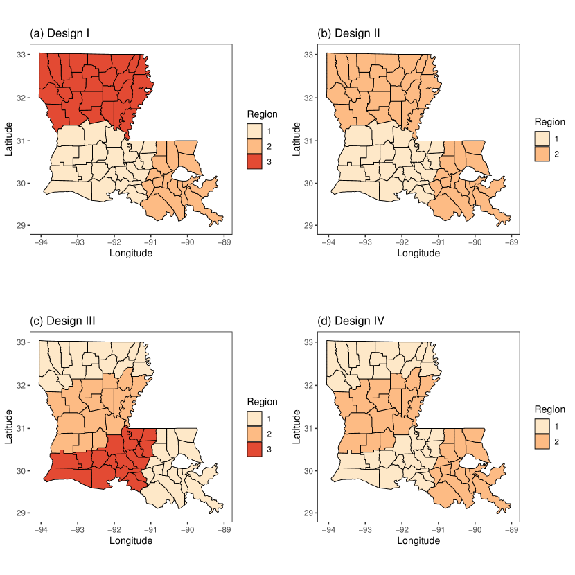
Figure 1: Geographical clustering patterns in Louisiana state of simulation designs (This figure appears in color in the electronic version of this article, and any mention of color refers to that version.)

For each design, 100 replicate datasets are generated under proportional hazards model with piecewise constant baseline hazard. In each replicate, we generate survival data of 60 subjects for each county, including three regression covariates from $N(0,1)$ i.i.d., survival time and censoring. We set three pieces for the baseline hazards with cutting points 1.5 and 6 for all designs, and over four designs, we have three true clusters at maximum, and the true regression coefficients and baseline hazards used are chosen from ${\mbox{\boldmath$\beta$}}_{1}=(1,0.5,1),{\mbox{\boldmath$\lambda$}}_{1}=(0.045,0.036,0.045)$, ${\mbox{\boldmath$\beta$}}_{2}=(1.5,1,1),{\mbox{\boldmath$\lambda$}}_{2}=(0.045,0.036,0.036)$, and ${\mbox{\boldmath$\beta$}}_{3}=(2,0.5,1.5),{\mbox{\boldmath$\lambda$}}_{3}=(0.036,0.045,0.0495)$. Censoring times are generated independently by taking the minimum of 150 and random values from Exp(0.01) with expectation 100. For each replicate, we set $\alpha=1$ and run different values of $h$, from 0 to 2 with grid 0.2, and from 3 to 10 with grid 1, and select the optimal $h$ via LPML. A total of 2000 MCMC iterations are run for each replicate, with the first 500 iterations as burn-in.

To compare the performance of clustering of gwCRP under different values of $h$, both estimation of the number of clusters and the matchability of clustering configurations are reported. In our simulation, we use mean Rand Index (Rand, 1971) which is obtained by using R-package fossil (Vavrek, 2011) to measure the clustering performance.

In addition to clustering performance, we further evaluate the estimation performance of covariates coefficients and baseline hazards, which is assessed by average of bias (AB) and average of mean squared error (AMSE) defined as follows. Let $\bm{z}=(z_{1},\ldots,z_{n})$ be the true clustering label vector, ${\mbox{\boldmath$\theta$}}_{r}(s_{i})$ be the true parameter value of cluster $r$, $\kappa_{r}=\sum_{i=1}^{64}{\bf{{1}}}(z_{i}=r)$ be the number of counties in cluster $r$, $r=1,\ldots,k$, $\sum_{r=1}^{k}\kappa_{r}=n$, and for simulated data set $t$, let $\widehat{{\mbox{\boldmath$\theta$}}}_{(t)}(s_{i})$ be Dahl’s method estimate at location $s_{i}$ for $t$-th replicates. Then AB is calculated as

$$\text{AB}=\frac{1}{k}\sum_{r=1}^{k}\frac{1}{\kappa_{r}}\sum_{i|z_{i}=r}\frac{1}{100}\sum_{t=1}^{100}(\widehat{{\mbox{\boldmath$\theta$}}}_{(t)}(s_{i})-{\mbox{\boldmath$\theta$}}_{r}(s_{i})),$$

and AMSE is calculated as

$$\text{AMSE}=\frac{1}{k}\sum_{r=1}^{k}\frac{1}{\kappa_{r}}\sum_{i|z_{i}=r}\frac{1}{100}\sum_{t=1}^{100}(\widehat{{\mbox{\boldmath$\theta$}}}_{(t)}(s_{i})-{\mbox{\boldmath$\theta$}}_{r}(s_{i}))^{2},$$

which calculates mean squared errors for each cluster first, and then average across clusters.

4.2 Simulation Results

Figure 2 shows the histogram of $k$ estimates and boxplots of Rand Index under different $h$ and the optimal selected by LPML for four simulation designs. We see that when $h=0$, the proposed gwCRP method is identical to the traditional CRP method, and in this case, CRP always tends to over-cluster and often yields smaller Rand Index than the results under $h>0$. Another important trend is that, as $h$ increases, the estimated number of clusters decreases first and then increases, and the Rand Index increases first and then decreases as $h$ becomes too large. As we discussed in Remark 1, this is because when $h$ increases from 0, the spatial patterns in the data is captured by the proposed gwCRP method. However, as $h\rightarrow\infty$, the geographical weights $w_{ij}$ for spatial-discontiguous counties become 0, which means only adjacent counties can be classified into the same cluster, therefore leading to over-clustering phenomenon again. It is also discovered that the clustering perfomance under optimal $h$ selected by LPML is very well, with the probability of selecting true number of clusters always greater than 0.75, and Rand Index larger than or similar to the highest results attained by some fixed value of $h$.

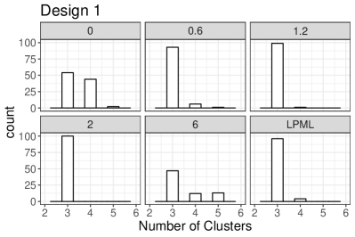
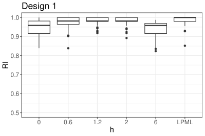
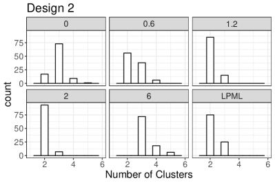
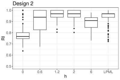
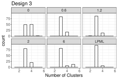
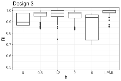
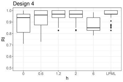
Figure 2: Histogram of estimates of $k$ and boxplot of Rand Index under different $h$ and LPML selection for simulation designs. The average h selected by LPML is 1.296 in Design 1, 1.412 in Design 2, 1.366 in Design 3, 1.602 in Design 4.

Table 1 summarizes the AB and AMSE results of estimating parameters of gwCRP under different $h$ for different designs. For simplicity of summary results, here the AMSE of $\beta$ is the average of AMSE of $\beta_{1},\beta_{2},\beta_{3}$ since they have similar scales, and the value of $\log{\mbox{\boldmath$\lambda$}}$ is the average of AMSE of $\log\lambda_{1},\log\lambda_{2},\log\lambda_{3}$, respectively.

For Designs II, III and IV, the absolute value of AB decrease as $h$ increase from 0 to moderate values, and increase again as $h$ increase to relatively large values. For all four designs, the absolute values of AB for $\lambda$’s of optimal $h$ selected by LPML always are the smallest, and the absolute values for both $\beta$’s and $\lambda$’s of optimal $h$ selected by LPML are always smaller than the values of traditional CRP. The patterns in AMSE are more clear when comparing different methods, that traditional CRP has the largest AMSE and AMSE decrease as $h$ increase from 0 to moderate values, and increase again as $h$ increase to relatively large values. The results of optimal $h$ selected by LPML also has the best performance in estimation.

Table 1: AB and AMSE for parameter estimation under different $h$ and LPML selection for different simulation designs

Method	Parameter	Design I		Design II		Design III		Design IV
		AB	AMSE	AB	AMSE	AB	AMSE	AB	AMSE
gwCRP $h=0.6$	$\beta$	-0.0063	0.0069	0.0038	0.0067	-0.0065	0.0083	-0.0027	0.0060
	$\lambda$	0.0815	0.0193	0.0732	0.0186	0.0797	0.0219	0.0827	0.0190
gwCRP $h=1.2$	$\beta$	-0.0078	0.0065	-0.0002	0.0058	-0.0061	0.0087	-0.0017	0.0049
	$\lambda$	0.0818	0.0194	0.0775	0.0171	0.0794	0.0217	0.0815	0.0172
gwCRP $h=2$	$\beta$	-0.0096	0.0068	-0.0006	0.0055	-0.0056	0.0085	-0.0051	0.0049
	$\lambda$	0.0849	0.0190	0.0814	0.0158	0.0798	0.0216	0.0873	0.0191
gwCRP $h=6$	$\beta$	-0.0061	0.0129	0.0030	0.0072	-0.0299	0.0204	-0.0064	0.0074
	$\lambda$	0.0805	0.0281	0.0770	0.0217	0.1005	0.0296	0.0852	0.0195
gwCRP Optimal	$\beta$	-0.0039	0.0059	0.0042	0.0055	0.0074	0.0067	-0.0005	0.0035
	$\lambda$	0.0661	0.0177	0.0711	0.0145	0.0732	0.0203	0.0777	0.0177
CRP	$\beta$	-0.0046	0.0086	0.0018	0.0092	-0.0056	0.0089	0.0003	0.0082
	$\lambda$	0.0760	0.0228	0.0717	0.0233	0.0787	0.0239	0.0742	0.0223

A sensitivity analysis regarding $\alpha$ and the weighting function is conducted. $\alpha=0.5,1,2,5$ and the weighting function $w_{ij}=\exp(-d_{v_{i}v_{j}}^{2}\times h^{2}){\bf{{1}}}\{d_{v_{i}v_{j}}>1\}+{\bf{{1}}}\{d_{v_{i}v_{j}}\leq 1\}$ which has a faster decay to 0 are ran, and all the results are presented in Section D of Supporting information. The results show that the results of optimal $h$ selected by LPML are insensitive to the choice of $\alpha$ and weighting function.

In a brief conclusion based on our simulation studies, gwCRP models have better performance than CRP both for clustering and parameter estimation. Our proposed model selection criterion, LPML, can nearly select the best performing $h$ value for both clustering and parameter estimation.

5 SEER Respiratory Cancer Data

5.1 Data Description

In this section, we apply our proposed model to analyze respiratory cancer data in Louisiana state, which is downloaded from the Surveillance, Epidemiology, and End Results (SEER) Program.We analyzed the survival time of respiratory cancer patients using the SEER public use data (SEER 1973-2016 Public-Use). We refer to Mu et al. (2020) for the detailed data clean description. After cleaning, there are 16213 observations left, and the censoring rate is 30.44%. We select Age, Gender, Cancer grade and Historical stage of cancer for our analysis, and give the summary of survival times and covariates in Table 2. The median survival times for patients in each county are provided in Section E of Supporting information .

Table 2: Demographics for the studied dataset. For continuous variables, the mean and standard deviation (SD) are reported. For binary variables, the frequency and percentage of each class are reported.

	Mean(SD) / Frequency (Percentage)
Survival Time	22.43 (31.90)
Event	12.63 (18.32)
Censor	44.85 (43.06)
Diagnostic Age	66.55 (11.66)
Sex
Female	6548 ($40.39\%$)
Male	9665 ($59.61\%$)
Cancer Grade
the class of lower grades	5307 ($32.73\%$)
the class of III or IV	10906 ($67.27\%$)
Historical Stage
not distant	9005 ($55.54\%$)
distant	7208 ($44.46\%$)

We first fit the Cox model of patients for each county using the covariates selected. The regression coefficients are visualized in Section E of Supporting information. From results shown in Supporting information, it is seen that some counties have similar characteristics, no limited to only adjacent counties, indicating possibilities of globally discontiguous clusters.

5.2 Data Analysis

To select the optimal number of pieces for the baseline hazard and $h$, we run $J=2$ with the cutpoints $(0,9.01)$, $J=3$ with cutpoints $(0,3.01,9.01)$, $J=4$ with cutpoints $(0,1.01,4.01,9.01)$, and $J=5$ with cutpoints $(0,1.01,3.01,5.01,9.01)$. The cutpoints are set by dividing the start point $0$ and the median survival time $9.01$ by quantiles evenly to ensure there are events at each piece for each county. For each $J$, we run $h$ from 0 to 10 with grid 0.1, and for each combination of $J$ and $h$, 5000 MCMC iterations are run and drop the first 2000 as burn-in. The optimal values selected by LPML is $J=4$ and $h=9.0$, under which the corresponding estimate of number of clusters is two, while the traditional CRP classifies the counties into five clusters. The trace plots of different chains of posterior samples of the estimates for selected counties are presented in the Section E of Supporting information to show the convergence of the MCMC. The plots of clustering patterns of CRP and gwCRP Optimal are shown in Figure 3, from which it is seen that the gwCRP captures the globally discontiguous clusters very well. The estimates and $95\%$ Credible Intervals of regression covariates coefficients and baseline hazards obtained by gwCRP Optimal are given in Table 3, from which we see that, though the baseline hazards are similar, the regression covariates coefficients are quite different across different clusters. We see that our proposed method successfully detects both spatially contiguous cluster and discontinuous cluster simultaneously. The parameter estimates for Age are positive in all counties, indicating that older patients on average are more likely to have the event than younger patients. For the counties in cluster 1, the diagnostic ages has higher hazards effects than other counties. However, for the counties in Cluster 2, male, later cancer stage will have higher hazards effects than other counties. The historical distance stage effects are very similar in two clusters which indicates that the subjects with tumor spreading will have higher hazards.

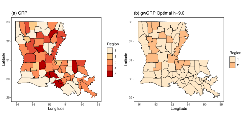
Figure 3: Clustering patterns of counties in Louisiana state under CRP (when J=4) and gwCRP Optimal (when J=4, h=9.0) methods (This figure appears in color in the electronic version of this article, and any mention of color refers to that version.)

Table 3: Estimates results of regression coefficients and baseline hazards obtained by gwCRP Optimal ($J=4,~{}h=9.0$). The $95\%$ Credible Interval for estimates of Cluster One is calculated by the $95\%$ HPD Interval of County 13, and The $95\%$ Credible Interval for estimates of Cluster Two is calculated by the $95\%$ HPD Interval of County 33, where the counties were selected by the minimum Euclidean distance from the posterior mean to the average estimate.

Parameter	Cluster 1		Cluster 2
	Estimate	$95\%$ Credible Interval	Estimate	$95\%$ Credible Interval
$\beta_{\text{Age}}$	0.1847	(0.1693, 0.2158)	0.0728	(0.0138, 0.2056)
$\beta_{\text{Sex}}$	0.1239	(0.0912, 0.1732)	0.3411	(0.1118, 0.5189)
$\beta_{\text{Grade}}$	0.5075	(0.4366, 0.5291)	0.8290	(0.4583, 0.9578)
$\beta_{\text{Hist-Stage}}$	1.3271	(1.2926, 1.3824)	1.4434	(1.3150, 1.7101)
$\lambda_{1}$	1.0690	(0.9938, 1.0912)	1.0359	(0.9060, 1.2330)
$\lambda_{2}$	1.0716	(0.9909, 1.1172)	1.0877	(0.8432, 1.3035)
$\lambda_{3}$	0.9843	(0.9787, 1.1040)	1.0912	(0.8535, 1.2899)
$\lambda_{4}$	1.0040	(0.9583, 1.0513)	1.0209	(0.8724, 1.2091)

6 Discussion

In this paper, we proposed a geographically weighted Chinese restaurant process to capture spatial homogeneity of regression coefficients and baseline hazards based on piecewise constant hazard model. An efficient MCMC algorithm is proposed for our methods without complicated reversible jump algorithm. Extensive simulation results are carried out to show that our proposed method has better clustering performance than the traditional CRP in spatial homogeneity pursuit for survival data. Simulation studies also show that our proposed methods have promising results in coefficients and baseline hazard estimation. An application to analysis of SEER data provides an interesting illustration of our proposed methods.

Furthermore, four topics beyond the scope of this paper are worth further investigation. In this paper, our proposed algorithm is based on two step estimation under piecewise constant proportional hazard model assumption. Proposing an efficient sampling algorithm without Laplace approximation is an important future work. Furthermore, we fixed the number of pieces of baseline hazards in both simulation studies and real data analysis. Imposing adaptive number of pieces model in baseline hazards is devoted for future research. In addition, variable selection approaches based on hierarchical CRP (Griffiths et al., 2004) is also worth being investigated. Allowing different covariates and baseline hazard share different clustering processes is also an important future work.

Data Availability Statement

The data that support the findings of this paper are available from the corresponding author upon reasonable request.

Supporting Information

Web Appendices, Tables, and Figures referenced in Sections 2-5 and R scripts for simulationsand real data examples are available with this paper at the Biometrics website on WileyOnline Library. The R code for the computations of this paper is available at https://github.com/lj-geng/GWCRP.

References

- Banerjee et al. (2014) Banerjee, S., Carlin, B. P., and Gelfand, A. E. (2014). Hierarchical modeling and analysis for spatial data. Crc Press.
- Banerjee and Dey (2005) Banerjee, S. and Dey, D. K. (2005). Semiparametric proportional odds models for spatially correlated survival data. Lifetime Data Analysis 11, 175–191.
- Banerjee et al. (2003) Banerjee, S., Wall, M. M., and Carlin, B. P. (2003). Frailty modeling for spatially correlated survival data, with application to infant mortality in Minnesota. Biostatistics 4, 123–142.
- Bhatt and Tiwari (2014) Bhatt, V. and Tiwari, N. (2014). A spatial scan statistic for survival data based on weibull distribution. Statistics in medicine 33, 1867–1876.
- Blackwell et al. (1973) Blackwell, D., MacQueen, J. B., et al. (1973). Ferguson distributions via pólya urn schemes. The Annals of Statistics 1, 353–355.
- Blei and Frazier (2011) Blei, D. M. and Frazier, P. I. (2011). Distance dependent Chinese restaurant processes. Journal of Machine Learning Research 12, 2461–2488.
- Chen et al. (2000) Chen, M.-H., Qi-Man, S., and G, I. J. (2000). Monte Carlo Methods in Bayesian Computation. New York: Springer-Verlag.
- Cox (1972) Cox, D. R. (1972). Regression models and life-tables. Journal of the Royal Statistical Society B 34, 187–220.
- Dahl (2006) Dahl, D. B. (2006). Model-based clustering for expression data via a Dirichlet process mixture model. Bayesian inference for gene expression and proteomics 4, 201–218.
- Friedman et al. (1982) Friedman, M. et al. (1982). Piecewise exponential models for survival data with covariates. The Annals of Statistics 10, 101–113.
- Geisser (1993) Geisser, S. (1993). Predictive Inference: An Introduction. London: Chapman & Hall.
- Gelfand and Dey (1994) Gelfand, A. E. and Dey, D. K. (1994). Bayesian model choice: asymptotics and exact calculations. Journal of the Royal Statistical Society: Series B (Methodological) 56, 501–514.
- Gelfand et al. (1992) Gelfand, A. E., Dey, D. K., and Chang, H. (1992). Model determination using predictive distributions with implementation via sampling-based-methods (with discussion). In In Bayesian Statistics 4. University Press.
- Gelfand et al. (2003) Gelfand, A. E., Kim, H.-J., Sirmans, C., and Banerjee, S. (2003). Spatial modeling with spatially varying coefficient processes. Journal of the American Statistical Association 98, 387–396.
- Green (1995) Green, P. J. (1995). Reversible jump Markov chain Monte Carlo computation and Bayesian model determination. Biometrika 82, 711–732.
- Griffiths et al. (2004) Griffiths, T. L., Jordan, M. I., Tenenbaum, J. B., and Blei, D. M. (2004). Hierarchical topic models and the nested Chinese restaurant process. In Advances in neural information processing systems, pages 17–24.
- Henderson et al. (2012) Henderson, R., Shimakura, S., and Gorst, D. (2012). Modeling spatial variation in leukemia survival data. Journal of the American Statistical Association .
- Hu et al. (2020) Hu, G., Geng, J., Xue, Y., and Sang, H. (2020). Bayesian spatial homogeneity pursuit of functional data: an application to the U.S. income distribution.
- Hu and Huffer (2020) Hu, G. and Huffer, F. (2020). Modified Kaplan–Meier estimator and Nelson–Aalen estimator with geographical weighting for survival data. Geographical Analysis 52, 28–48.
- Hu et al. (2020) Hu, G., Xue, Y., and Huffer, F. (2020). A comparison of Bayesian accelerated failure time models with spatially varying coefficients. Sankhya B pages 1–17.
- Huang et al. (2007) Huang, L., Pickle, L. W., Stinchcomb, D., and Feuer, E. J. (2007). Detection of spatial clusters: application to cancer survival as a continuous outcome. Epidemiology 18, 73–87.
- Ibrahim et al. (2001) Ibrahim, J. G., Chen, M.-H., and Sinha, D. (2001). Bayesian Survival Analysis. New York: Springer-Verlag.
- Lee et al. (2017) Lee, J., Gangnon, R. E., and Zhu, J. (2017). Cluster detection of spatial regression coefficients. Statistics in Medicine 36, 1118–1133.
- Lee et al. (2019) Lee, J., Sun, Y., and Chang, H. H. (2019). Spatial cluster detection of regression coefficients in a mixed-effects model. Environmetrics page e2578.
- Li and Sang (2019) Li, F. and Sang, H. (2019). Spatial homogeneity pursuit of regression coefficients for large datasets. Journal of the American Statistical Association pages 1–21.
- Lu et al. (2018) Lu, J., Li, M., and Dunson, D. (2018). Reducing over-clustering via the powered Chinese restaurant process. arXiv preprint arXiv:1802.05392 .
- Ma et al. (2020) Ma, Z., Xue, Y., and Hu, G. (2020). Heterogeneous regression models for clusters of spatial dependent data. Spatial Economic Analysis 15, 459–475.
- Miller and Harrison (2013) Miller, J. W. and Harrison, M. T. (2013). A simple example of Dirichlet process mixture inconsistency for the number of components. In Advances in Neural Information Processing Systems, pages 199–206.
- Mu et al. (2020) Mu, J., Liu, Q., Kuo, L., and Hu, G. (2020). Bayesian variable selection for cox regression model with spatially varying coefficients with applications to louisiana respiratory cancer data. arXiv preprint arXiv:2008.00615 .
- Neal (2000) Neal, R. M. (2000). Markov chain sampling methods for Dirichlet process mixture models. Journal of Computational and Graphical Statistics 9, 249–265.
- Pitman (1995) Pitman, J. (1995). Exchangeable and partially exchangeable random partitions. Probability Theory and Related Fields 102, 145–158.
- Rand (1971) Rand, W. M. (1971). Objective criteria for the evaluation of clustering methods. Journal of the American Statistical Association 66, 846–850.
- SEER (2016) SEER, P. (2016). Public-use data (1973-2015). national cancer institute, dccps, surveillance research program, cancer statistics branch, released april 2016, based on the november 2015 submission.
- Tobler (1970) Tobler, W. R. (1970). A computer movie simulating rrban growth in the Detroit region. Economic Geography 46, 234–240.
- Vavrek (2011) Vavrek, M. J. (2011). Fossil: palaeoecological and palaeogeographical analysis tools. Palaeontologia Electronica 14, 16.
- Xue et al. (2020) Xue, Y., Schifano, E. D., and Hu, G. (2020). Geographically weighted Cox regression for prostate cancer survival data in Louisiana. Geographical Analysis 52, 570–587.
- Zhang and Lawson (2011) Zhang, J. and Lawson, A. B. (2011). Bayesian parametric accelerated failure time spatial model and its application to prostate cancer. Journal of Applied Statistics 38, 591–603.
- Zhao et al. (2020) Zhao, P., Yang, H.-C., Dey, D. K., and Hu, G. (2020). Bayesian spatial homogeneity pursuit regression for count value data. arXiv preprint arXiv:2002.06678 .
- Zhou et al. (2008) Zhou, H., Lawson, A. B., Hebert, J. R., Slate, E. H., and Hill, E. G. (2008). Joint spatial survival modeling for the age at diagnosis and the vital outcome of prostate cancer. Statistics in Medicine 27, 3612–3628.