Dehn colorings and vertex-weight invariants for spatial graphs

Abstract.

In this paper, we study Dehn colorings for spatial graphs, and give a family of spatial graph invariants that are called vertex-weight invariants. We give some examples of spatial graphs that can be distinguished by a vertex-weight invariant, whereas distinguished by neither their constituent links nor the number of Dehn colorings.

Introduction

Fox colorings for classical links have been used by various studies in knot theory, see [2, 10, 11] for example. In [3], Fox colorings for spatial graph diagrams were studied with two kinds of vertex conditions, and in [8], vertex conditions for Fox colorings of spatial graph diagrams were completely classified with “some invariants for an equivalence relation on $\sum_{n\in 2\mathbb{Z}_{+}}\mathbb{Z}_{p}^{n}$”. We note that the classification gives the maximum generalization for Fox colorings of spatial graph diagrams unless we change the fundamental definition that a Fox $p$-coloring of a diagram $D$ is a map $C:\{\mbox{arcs of $D$}\}\to\mathbb{Z}_{p}$ satisfying the crossing condition depicted in Figure 1. Dehn colorings, namely region colorings by $\mathbb{Z}_{p}$, for classical links have been also studied in knot theory, see [1, 5, 7] for example. In particular, in [1], some relation between Fox colorings and Dehn colorings was given.

In this paper, we study Dehn colorings for spatial graph diagrams, and we discuss about “some invariants for an equivalence relation on $\sum_{n\in 2\mathbb{Z}_{+}}\mathbb{Z}_{p}^{n}$” related to Dehn colorings of spatial graph diagrams. Note that as in the case of Fox colorings of spatial graph diagrams, the invariants can be used for the classification of vertex conditions for Dehn colorings of spatial graph diagrams, which will be studied in our next paper [9]. Furthermore, we show each invariant for the equivalence relation on $\sum_{n\in 2\mathbb{Z}_{+}}\mathbb{Z}_{p}^{n}$ gives a spatial graph invariant called a vertex-weight invariant. We give some examples of spatial graphs that can be distinguished by a vertex-weight invariant, whereas distinguished by neither their constituent links nor the number of Dehn colorings. Note that the notion of a vertex-weight invariant discussed in this paper can be also applied for the case of Fox colorings of spatial graphs.

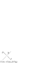
Figure 1.

This paper is organized as follows: In Section 1, we introduce an equivalence relation on $\sum_{n\in 2\mathbb{Z}_{+}}\mathbb{Z}_{p}^{n}$, and discuss some invariants under the equivalence relation. In Section 2, we review the definitions of spatial graphs and their diagrams. In Section 3, a Dehn coloring of a spatial Euler graph diagram is defined. Section 4 is devoted to the study of vertex-weight invariants of spatial Euler graphs, and presents some example of spatial Euler graphs that can be distinguished by a vertex-weight invariant, whereas distinguished by neither their constituent links nor the number of Dehn colorings. Section 5 deals with the case of spatial graphs each of which includes an odd-valent vertex, and presents some example of spatial graphs that can be distinguished by a vertex-weight invariant, whereas distinguished by neither their constituent links nor the number of Dehn colorings.

1. Invariants of an equivalence relation on $\sum_{n\in 2\mathbb{Z}_{+}}\mathbb{Z}_{p}^{n}$

Throughout this paper, $\mathbb{Z}_{+}$ means the set of positive integers, $\mathbb{Z}_{\geq q}$ means the set of integers greater than or equal to $q$, and $\mathbb{Z}_{p}=\{0,1,\ldots,p-1\}$ means the cyclic group $\mathbb{Z}/p\mathbb{Z}$.

From now on, let $p\in\mathbb{Z}_{\geq 2}$, and put $U_{p}=\bigcup_{n\in 2\mathbb{Z}_{+}}\mathbb{Z}^{n}_{p}$.

Definition 1.1.

Two elements $\displaystyle\bm{a},\bm{b}\in U_{p}$ are equivalent ($\bm{a}\sim\bm{b}$) if $\bm{a}$ and $\bm{b}$ are related by a finite sequence of the following transformations:

• $(a_{1},\ldots,a_{n})\longrightarrow(a_{2},\ldots,a_{n},a_{1})$,

• $(a_{1},\ldots,a_{n})\longrightarrow(a,a_{2}+(-1)^{2}(a_{1}-a),\ldots,a_{i}+(-1)^{i}(a_{1}-a),\ldots,a_{n}+(-1)^{n}(a_{1}-a))$ for $a\in\mathbb{Z}_{p}$,

• $(a_{1},\ldots,a_{n})\longrightarrow(a,a_{1}-a_{2}+a,\ldots,a_{1}-a_{i}+a,\ldots,a_{1}-a_{n}+a)$ for $a\in\mathbb{Z}_{p}$,

• $(a_{1},\ldots,a_{n})\longrightarrow(a_{1},-a_{1}+a_{2}+a_{3},a_{3},\ldots,a_{n})$ when $n>3$.

Remark 1.2.

The inverse of (Op1) is (Op1)^n-1. The inverse of (Op2) is (Op2) for $a=a_{1}\in\mathbb{Z}_{p}$. The inverse of (Op3) is (Op3) for $a=a_{1}\in\mathbb{Z}_{p}$. The inverse of (Op4) is (Op4)^p-1.

Put $\bm{a}=(a_{1},\ldots,a_{n})$. We define $\displaystyle\tau_{p}:U_{p}\longrightarrow\mathbb{Z}$ by

$$\tau_{p}\big{(}\bm{a}\big{)}=\max\left\{k\in\{1,\ldots,p\}~{}{\Bigg{|}}~{}\begin{array}[]{l}\ k|p,\\ a_{1}+a_{2}\equiv a_{2}+a_{3}\equiv\cdots\equiv a_{n}+a_{1}\pmod{k}\end{array}\right\}.$$

Suppose $p$ is an even integer. We define $\displaystyle\varepsilon_{p}:U_{p}\longrightarrow\mathbb{Z}\cup\{\infty\}$ by

$$\varepsilon_{p}\big{(}\bm{a}\big{)}=\begin{cases}0&\mbox{if }a_{1}+a_{2}\equiv\cdots\equiv a_{n}+a_{1}\equiv 0\pmod{2},\\ 1&\mbox{if }a_{1}+a_{2}\equiv\cdots\equiv a_{n}+a_{1}\equiv 1\pmod{2},\\ \infty&{\rm otherwise.}\end{cases}$$

We define $\displaystyle\mu_{p}:U_{p}\longrightarrow\mathbb{Z}$ by

$$\mu_{p}\big{(}\bm{a}\big{)}=E(a_{1}+a_{2},\ldots,a_{n}+a_{1})-O(a_{1}+a_{2},\ldots,a_{n}+a_{1}),$$

where

$$E\big{(}\bm{a}\big{)}=\#\{i\in\{1,\ldots,n\}\mid a_{i}\equiv 0\pmod{2}\}$$

and

$$O\big{(}\bm{a}\big{)}=\#\{i\in\{1,\ldots,n\}\mid a_{i}\equiv 1\pmod{2}\}.$$

For $\tau\in\{1,\ldots,p\}$ such that $\tau\equiv 0\pmod{2}$, $\tau|p$ and $\displaystyle\frac{p}{\tau}\equiv 0\pmod{2}$, define $\displaystyle\mu_{p,\tau}:U_{p}\longrightarrow\mathbb{Z}\cup\{\infty\}$ by

$$\mu_{p,\tau}\big{(}\bm{a}\big{)}=\begin{cases}\displaystyle~{}{\Bigg{|}}~{}\mu_{\frac{p}{\tau}}\Big{(}\frac{a_{1}-a_{1}}{\tau},\ldots,\frac{a_{2j-1}-a_{1}}{\tau},\frac{a_{2j}-a_{2}}{\tau},\ldots,\frac{a_{n}-a_{2}}{\tau}\Big{)}~{}{\Bigg{|}}&\mbox{if }\tau_{p}(\bm{a})=\tau,\\ \hskip 85.35826pt\infty&{\rm otherwise.}\end{cases}$$

Remark 1.3.

$\mu_{p,\tau}$ is well-defined since $a_{2j-1}-a_{1}\equiv 0\pmod{\tau}$ and $a_{2j}-a_{2}\equiv 0\pmod{\tau}$ for $j\in\{2,\ldots,\frac{n}{2}\}$ when $\tau_{p}\big{(}\bm{a}\big{)}=\tau$.

We have the following theorems.

Theorem 1.4.

Let ${\bm{a}}$ and ${\bm{b}}$ be two equivalent elements of $U_{p}$. Then it holds that $\tau_{p}(\bm{a})=\tau_{p}(\bm{b})$.

Proof.

It suffices to show that $\tau_{p}$ is an invariant under the transformations (Op1)-(Op4) in Definition 1.1.

(Op1) It is easy to see that

$$\tau_{p}(a_{2},\ldots,a_{n},a_{1})=\tau_{p}(a_{1},\ldots,a_{n})$$

for $(a_{1},\ldots,a_{n})\in U_{p}$.

(Op2) For $(a_{1},\ldots,a_{n})\in U_{p}$, $a\in\mathbb{Z}_{p}$ and $k\in\{1,2,\ldots,p\}$ such that $k|p$, we have

$$a_{1}+a_{2}\equiv a_{2}+a_{3}\equiv\cdots\equiv a_{n}+a_{1}\pmod{k}$$

$$\iff a+a_{2}+(-1)^{2}(a_{1}-a)\equiv\cdots\equiv a_{i}+(-1)^{i}(a_{1}-a)+a_{i+1}+(-1)^{i+1}(a_{1}-a)$$

$$\hskip 28.45274pt\equiv\cdots\equiv a_{n}+(-1)^{n}(a_{1}-a)+a\pmod{k}.$$

Hence

$$\tau_{p}\big{(}a_{1},\ldots,a_{n}\big{)}=\tau_{p}\big{(}a,a_{2}+(a_{1}-a),\ldots,a_{i}+(-1)^{i}(a_{1}-a),\ldots,a_{n}+(a_{1}-a)\big{)}$$

holds.

(Op3) For $(a_{1},\ldots,a_{n})\in U_{p}$, $a\in\mathbb{Z}_{p}$ and $k\in\{1,2,\ldots,p\}$ such that $k|p$, we have

$$a_{1}+a_{2}\equiv a_{2}+a_{3}\equiv\cdots\equiv a_{n}+a_{1}\pmod{k}$$

$$\iff 2a_{1}-(a_{1}+a_{2})+2a\equiv\cdots\equiv 2a_{1}-(a_{i}+a_{i+1})+2a$$

$$\hskip 28.45274pt\equiv\cdots\equiv 2a_{1}-(a_{n}+a_{1})+2a\pmod{k}.$$

$$\iff a+(a_{1}-a_{2}+a)\equiv\cdots\equiv(a_{1}-a_{i}+a)+(a_{1}-a_{i+1}+a)$$

$$\hskip 28.45274pt\equiv\cdots\equiv(a_{1}-a_{n}+a)+a\pmod{k}.$$

Hence

$$\tau_{p}(a_{1},\ldots,a_{n})=\tau_{p}(a,a_{1}-a_{2}+a,\ldots,a_{1}-a_{i}+a,\ldots,a_{1}-a_{n}+a)$$

holds.

(Op4) For $(a_{1},\ldots,a_{n})\in\displaystyle U_{p}$ and $k\in\{1,2,\ldots,p\}$ such that $n>3$ and $k|p$, since

$$a_{1}+a_{2}\equiv a_{2}+a_{3}\pmod{k}\iff-(a_{1}+a_{2})+(a_{2}+a_{3})\equiv 0\pmod{k},$$

we have

$$a_{1}+a_{2}\equiv a_{2}+a_{3}\equiv\cdots\equiv a_{n}+a_{1}\pmod{k}$$

$$\iff a_{1}+a_{2}+\{-(a_{1}+a_{2})+(a_{2}+a_{3})\}\equiv a_{2}+a_{3}+\{-(a_{1}+a_{2})+(a_{2}+a_{3})\}$$

$$\hskip 25.60747pt\equiv a_{3}+a_{4}\equiv\cdots\equiv a_{n}+a_{1}\pmod{k}$$

$$\iff a_{2}+a_{3}\equiv(-a_{1}+a_{2}+a_{3})+a_{3}\equiv a_{3}+a_{4}\equiv\cdots\equiv a_{n}+a_{1}\pmod{k}$$

$$\iff a_{1}+(-a_{1}+a_{2}+a_{3})\equiv(-a_{1}+a_{2}+a_{3})+a_{3}\equiv\cdots\equiv a_{n}+a_{1}\pmod{k}.$$

Hence

$$\tau_{p}(a_{1},\ldots,a_{n})=\tau_{p}(a_{1},-a_{1}+a_{2}+a_{3},a_{3},\ldots,a_{n})$$

holds. ∎

Theorem 1.5.

Suppose $p$ is an even integer. Let ${\bm{a}}$ and ${\bm{b}}$ be two equivalent elements of $U_{p}$. Then it holds that $\varepsilon_{p}(\bm{a})=\varepsilon_{p}(\bm{b})$.

Proof.

It suffices to show that $\varepsilon_{p}$ is an invariant under the transformations (Op1)-(Op4) in Definition 1.1.

(Op1) It is easy to see that

$$\varepsilon_{p}(a_{2},\ldots,a_{n},a_{1})=\varepsilon_{p}(a_{1},\ldots,a_{n})$$

for $(a_{1},\ldots,a_{n})\in\displaystyle U_{p}$.

(Op2) For $(a_{1},\ldots,a_{n})\in U_{p}$ and $a\in\mathbb{Z}_{p}$, we have

$$\varepsilon_{p}(a_{1},\ldots,a_{n})=\varepsilon$$

$$\iff{}^{\forall}i\in\{1,\ldots,n\},a_{i}+a_{i+1}\equiv\varepsilon\pmod{2}$$

$$\iff{}^{\forall}i\in\{1,\ldots,n\},\big{(}a_{i}+(-1)^{i}(a_{1}-a)\big{)}+\big{(}a_{i+1}+(-1)^{i+1}(a_{1}-a)\big{)}\equiv\varepsilon\pmod{2}$$

$$\iff\varepsilon_{p}\big{(}a,a_{2}+(-1)^{2}(a_{1}-a),\ldots,a_{i}+(-1)^{i}(a_{1}-a),\ldots,a_{n}+(-1)^{n}(a_{1}-a)\big{)}=\varepsilon$$

for $\varepsilon\in\{0,1\}$, where $a_{n+1}=a_{1}$.

(Op3) For $(a_{1},\ldots,a_{n})\in U_{p}$ and $a\in\mathbb{Z}_{p}$, we have

$$\varepsilon_{p}(a_{1},\ldots,a_{n})=\varepsilon$$

$$\iff{}^{\forall}i\in\{1,\ldots,n\},a_{i}+a_{i+1}\equiv\varepsilon\pmod{2}$$

$$\iff{}^{\forall}i\in\{1,\ldots,n\},\big{(}a_{1}-a_{i}+a\big{)}+\big{(}a_{1}-a_{i+1}+a\big{)}\equiv a_{i}+a_{i+1}\equiv\varepsilon\pmod{2}$$

$$\iff\varepsilon_{p}(a,a_{1}-a_{2}+a,\ldots,a_{1}-a_{i}+a,\ldots,a_{1}-a_{n}+a)=\varepsilon$$

for $\varepsilon\in\{0,1\}$, where $a_{n+1}=a_{1}$.

(Op4) For $(a_{1},\ldots,a_{n})\in\displaystyle U_{p}$ such that $n>3$, we have

$$\varepsilon_{p}(a_{1},\ldots,a_{n})=\varepsilon$$

$$\iff{}^{\forall}i\in\{1,\ldots,n\},a_{i}+a_{i+1}\equiv\varepsilon\pmod{2}$$

$$\iff a_{1}+(-a_{1}+a_{2}+a_{3})=a_{2}+a_{3}\equiv\varepsilon\pmod{2},$$

$$\hskip 28.45274pt(-a_{1}+a_{2}+a_{3})+a_{3}\equiv a_{1}+a_{2}\equiv\varepsilon\pmod{2},$$

$$\hskip 28.45274pt{}^{\forall}i\in\{3,\ldots,n\},a_{i}+a_{i+1}\equiv\varepsilon\pmod{2}$$

$$\iff\varepsilon_{p}(a_{1},-a_{1}+a_{2}+a_{3},a_{3},\ldots,a_{n})=\varepsilon$$

for $\varepsilon\in\{0,1\}$, where $a_{n+1}=a_{1}$.

∎

Theorem 1.6.

Suppose $p$ is an even integer. Let ${\bm{a}}$ and ${\bm{b}}$ be two equivalent elements of $U_{p}$. Then it holds that $\mu_{p}(\bm{a})=\mu_{p}(\bm{b})$.

Proof.

It suffices to show that $\mu_{p}$ is an invariant under the transformations (Op1)-(Op4) in Definition 1.1.

(Op1) It is easy to see that

$$\mu_{p}(a_{2},\ldots,a_{n},a_{1})=\mu_{p}(a_{1},\ldots,a_{n})$$

for $(a_{1},\ldots,a_{n})\in\displaystyle U_{p}$.

(Op2) For $(a_{1},\ldots,a_{n})\in\displaystyle U_{p}$ and $a\in\mathbb{Z}_{p}$, we have

$$\mu_{p}(a_{1},\ldots,a_{n})$$

$$=E(a_{1}+a_{2},\ldots,a_{n}+a_{1})-O(a_{1}+a_{2},\ldots,a_{n}+a_{1})$$

$$=E\big{(}a+a_{2}+(a_{1}-a),\ldots,(a_{i}+(-1)^{i}(a_{1}-a))+(a_{i+1}+(-1)^{i+1}(a_{1}-a)),$$

$$\hskip 256.0748pt\ldots,a_{n}+(a_{1}-a)+a\big{)}$$

$$\quad-O\big{(}a+a_{2}+(a_{1}-a),\ldots,(a_{i}+(-1)^{i}(a_{1}-a))+(a_{i+1}+(-1)^{i+1}(a_{1}-a)),$$

$$\hskip 256.0748pt\ldots,a_{n}+(a_{1}-a)+a\big{)}$$

$$=\mu_{p}(a,a_{2}+(a_{1}-a),\ldots,a_{i}+(-1)^{i}(a_{1}-a),\ldots,a_{n}+(a_{1}-a)).$$

(Op3) For $(a_{1},\ldots,a_{n})\in\displaystyle U_{p}$ and $a\in\mathbb{Z}_{p}$, we have

$$\mu_{p}(a_{1},\ldots,a_{n})$$

$$=E(a_{1}+a_{2},\ldots,a_{n}+a_{1})-O(a_{1}+a_{2},\ldots,a_{n}+a_{1})$$

$$=E\big{(}2a_{1}-(a_{1}+a_{2})+2a,\ldots,2a_{1}-(a_{i}+a_{i+1})+2a,\ldots,2a_{1}-(a_{n}+a_{1})+2a\big{)}$$

$$\quad-O\big{(}2a_{1}-(a_{1}+a_{2})+2a,\ldots,2a_{1}-(a_{i}+a_{i+1})+2a,\ldots,2a_{1}-(a_{n}+a_{1})+2a\big{)}$$

$$=E\big{(}a+(a_{1}-a_{2}+a),\ldots,(a_{1}-a_{i}+a)+(a_{1}-a_{i+1}+a),\ldots,(a_{1}-a_{n}+a)+a\big{)}$$

$$\quad-O\big{(}a+(a_{1}-a_{2}+a),\ldots,(a_{1}-a_{i}+a)+(a_{1}-a_{i+1}+a),\ldots,(a_{1}-a_{n}+a)+a\big{)}$$

$$=\mu_{p}(a,a_{1}-a_{2}+a,\ldots,a_{1}-a_{i}+a,\ldots,a_{1}-a_{n}+a).$$

(Op4) For $(a_{1},\ldots,a_{n})\in U_{p}$ such that $n>3$, we have

$$\mu_{p}(a_{1},\ldots,a_{n})$$

$$=E(a_{1}+a_{2},\ldots,a_{n}+a_{1})-O(a_{1}+a_{2},\ldots,a_{n}+a_{1})$$

$$=E\big{(}a_{2}+a_{3},-(a_{1}+a_{2})+2(a_{2}+a_{3}),a_{3}+a_{4},\ldots,a_{n}+a_{1}\big{)}$$

$$\quad-O\big{(}a_{2}+a_{3},-(a_{1}+a_{2})+2(a_{2}+a_{3}),a_{3}+a_{4},\ldots,a_{n}+a_{1}\big{)}$$

$$=E\big{(}a_{1}+(-a_{1}+a_{2}+a_{3}),(-a_{1}+a_{2}+a_{3})+a_{3},a_{3}+a_{4},\ldots,a_{n}+a_{1}\big{)}$$

$$\quad-O\big{(}a_{1}+(-a_{1}+a_{2}+a_{3}),(-a_{1}+a_{2}+a_{3})+a_{3},a_{3}+a_{4},\ldots,a_{n}+a_{1}\big{)}$$

$$=\mu_{p}(a_{1},-a_{1}+a_{2}+a_{3},a_{3},\ldots,a_{n}).$$

∎

Theorem 1.7.

Suppose $p$ is an even integer. Let $\tau\in\{1,\ldots,p\}$ such that $\tau\equiv 0\pmod{2}$, $\tau|p$ and $\displaystyle\frac{p}{\tau}\equiv 0\pmod{2}$. Let ${\bm{a}}$ and ${\bm{b}}$ be two equivalent elements of $\displaystyle U_{p}$. Then it holds that $\mu_{p,\tau}(\bm{a})=\mu_{p,\tau}(\bm{b})$.

Proof.

It suffices to show that $\mu_{p,\tau}$ is an invariant under the transformations (Op1)-(Op4) in Definition 1.1.

(Op1) It is easy to see that

$$\mu_{p,\tau}(a_{2},\ldots,a_{n},a_{1})=\mu_{p,\tau}(a_{1},\ldots,a_{n})$$

for $(a_{1},\ldots,a_{n})\in\displaystyle U_{p}$.

(Op2) For $(a_{1},\ldots,a_{n})\in\displaystyle U_{p}$ and $a\in\mathbb{Z}_{p}$, we have

$$\mu_{p,\tau}(a_{1},\ldots,a_{n})$$

$$=~{}{\Big{|}}~{}\mu_{\frac{p}{\tau}}\Big{(}\frac{a_{1}-a_{1}}{\tau},\ldots,\frac{a_{2j-1}-a_{1}}{\tau},\frac{a_{2j}-a_{2}}{\tau},\ldots,\frac{a_{n}-a_{2}}{\tau}\Big{)}~{}{\Big{|}}$$

$$=~{}{\Big{|}}~{}\mu_{\frac{p}{\tau}}\Big{(}\ldots,\frac{(a_{2j-1}-(a_{1}-a))-a}{\tau},\frac{(a_{2j}+(a_{1}-a))-(a_{2}+(a_{1}-a))}{\tau},\ldots\Big{)}~{}{\Big{|}}$$

$$=\mu_{p,\tau}\big{(}a,a_{2}+(a_{1}-a),\ldots,a_{i}+(-1)^{i}(a_{1}-a),\ldots,a_{n}+(a_{1}-a)\big{)}.$$

(Op3) For $(a_{1},\ldots,a_{n})\in\displaystyle U_{p}$ and $a\in\mathbb{Z}_{p}$, we have

$$\mu_{p,\tau}(a_{1},\ldots,a_{n})$$

$$=~{}{\Big{|}}~{}\mu_{\frac{p}{\tau}}\Big{(}\frac{a_{1}-a_{1}}{\tau},\ldots,\frac{a_{2j-1}-a_{1}}{\tau},\frac{a_{2j}-a_{2}}{\tau},\ldots,\frac{a_{n}-a_{2}}{\tau}\Big{)}~{}{\Big{|}}$$

$$=~{}{\Big{|}}~{}\mu_{\frac{p}{\tau}}\Big{(}\frac{a_{1}-a_{1}}{\tau},\ldots,\frac{a_{1}-a_{2j-1}}{\tau},\frac{a_{2}-a_{2j}}{\tau},\ldots,\frac{a_{2}-a_{n}}{\tau}\Big{)}~{}{\Big{|}}$$

$$=~{}{\Big{|}}~{}\mu_{\frac{p}{\tau}}\Big{(}\ldots,\frac{(a_{1}-a_{2j-1}+a)-a}{\tau},\frac{(a_{1}-a_{2j}+a)-(a_{1}-a_{2}+a)}{\tau},\ldots\Big{)}~{}{\Big{|}}$$

$$=\mu_{p,\tau}(a,a_{1}-a_{2}+a,\ldots,a_{1}-a_{i}+a,\ldots,a_{1}-a_{n}+a).$$

(Op4) For $(a_{1},\ldots,a_{n})\in U_{p}$ such that $n>3$, we have

$$\mu_{p,\tau}(a_{1},\ldots,a_{n})$$

$$=~{}{\Big{|}}~{}\mu_{\frac{p}{\tau}}\Big{(}\frac{a_{1}-a_{1}}{\tau},\ldots,\frac{a_{2j-1}-a_{1}}{\tau},\frac{a_{2j}-a_{2}}{\tau},\ldots,\frac{a_{n}-a_{2}}{\tau}\Big{)}~{}{\Big{|}}$$

$$=~{}{\Big{|}}~{}E\Big{(}\ldots,\frac{a_{2j-1}-a_{1}}{\tau}+\frac{a_{2j}-a_{2}}{\tau},\frac{a_{2j}-a_{2}}{\tau}+\frac{a_{2j+1}-a_{1}}{\tau},\ldots\Big{)}$$

$$\quad-O\Big{(}\ldots,\frac{a_{2j-1}-a_{1}}{\tau}+\frac{a_{2j}-a_{2}}{\tau},\frac{a_{2j}-a_{2}}{\tau}+\frac{a_{2j+1}-a_{1}}{\tau},\ldots\Big{)}~{}{\Big{|}}~{}$$

$$=~{}{\Big{|}}~{}E\Big{(}\ldots,\frac{a_{2j-1}-a_{1}}{\tau}+(\frac{a_{2j}-a_{2}}{\tau}-\frac{a_{3}-a_{1}}{\tau}),$$

$$\hskip 170.71652pt(\frac{a_{2j}-a_{2}}{\tau}-\frac{a_{3}-a_{1}}{\tau})+\frac{a_{2j+1}-a_{1}}{\tau},\ldots\Big{)}$$

$$\quad-O\Big{(}\ldots,\frac{a_{2j-1}-a_{1}}{\tau}+(\frac{a_{2j}-a_{2}}{\tau}-\frac{a_{3}-a_{1}}{\tau}),$$

$$\hskip 170.71652pt(\frac{a_{2j}-a_{2}}{\tau}-\frac{a_{3}-a_{1}}{\tau})+\frac{a_{2j+1}-a_{1}}{\tau},\ldots\Big{)}~{}{\Big{|}}~{}$$

$$=~{}{\Big{|}}~{}\mu_{\frac{p}{\tau}}\Big{(}\frac{a_{1}-a_{1}}{\tau},\ldots,\frac{a_{2j-1}-a_{1}}{\tau},\frac{a_{2j}-a_{2}}{\tau}-\frac{a_{3}-a_{1}}{\tau},\ldots,\frac{a_{n}-a_{2}}{\tau}-\frac{a_{3}-a_{1}}{\tau}\Big{)}~{}{\Big{|}}$$

$$=~{}{\Big{|}}~{}\mu_{\frac{p}{\tau}}\Big{(}\frac{a_{1}-a_{1}}{\tau},\ldots,\frac{a_{2j-1}-a_{1}}{\tau},\frac{a_{2j}-(-a_{1}+a_{2}+a_{3})}{\tau},$$

$$\hskip 227.62204pt\ldots,\frac{a_{n}-(-a_{1}+a_{2}+a_{3})}{\tau}\Big{)}~{}{\Big{|}}$$

$$=\mu_{p,\tau}(a_{1},-a_{1}+a_{2}+a_{3},a_{3},\ldots,a_{n}).$$

∎

2. Spatial graph diagrams

A spatial graph is a graph embedded in $\mathbb{R}^{3}$. We call a spatial graph each of whose vertices is of even valence a spatial Euler graph. In this paper, a spatial graph means an unoriented spatial graph. Two spatial graphs are equivalent if we can deform by an ambient isotopy of $\mathbb{R}^{3}$ one onto the other. A diagram of a spatial graph $G$ is an image of $G$ by a regular projection onto $\mathbb{R}^{2}$ with a height information at each crossing point. It is known that two spatial graph diagrams represent an equivalent spatial graph if and only if they are related by a finite sequence of the Reidemeister moves of type I-V depicted in Figure 2. We call each connected component of complementary regions of a diagram a region of the diagram.

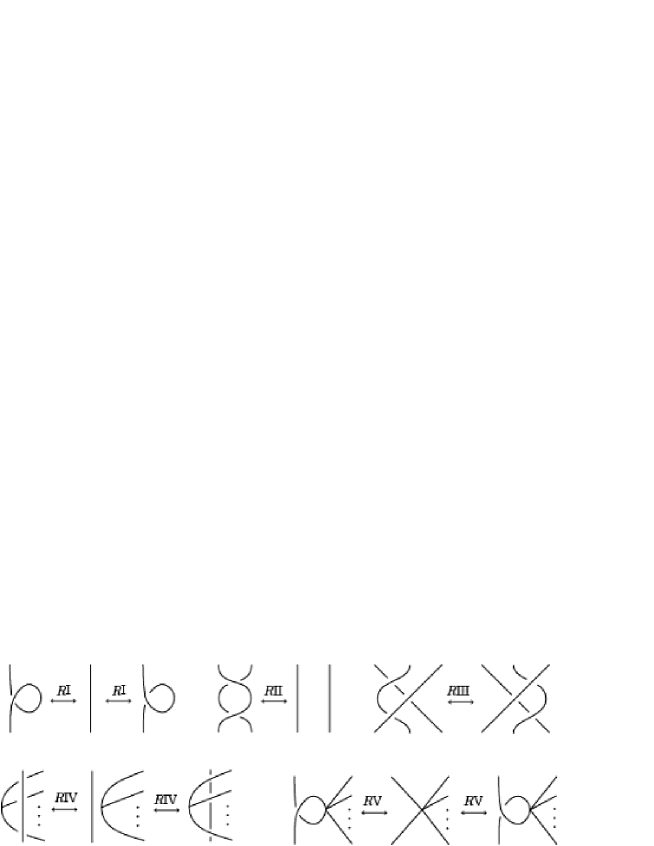
Figure 2.

3. Dehn $p$-colorings of diagrams of spatial Euler graphs

Definition 3.1.

Let $D$ be a diagram of a spatial Euler graph and $\mathcal{R}(D)$ the set of regions of $D$. A Dehn $p$-coloring of $D$ is a map $C:\mathcal{R}(D)\to\mathbb{Z}_{p}$ satisfying the following condition:

• For a crossing $c$ with regions $r_{1},r_{2},r_{3}$ and $r_{4}$ such that $r_{2}$ is adjacent to an arbitrary chosen $r_{1}$ by an under-arc and $r_{3}$ is adjacent to $r_{1}$ by the over-arc as depicted in Figure 3,

  $$C(r_{1})-C(r_{2})+C(r_{3})-C(r_{4})=0$$

  holds, which we call the crossing condition.

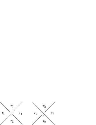
Figure 3.

We call $C(r)$ the color of a region $r$. We denote by ${\rm Col}_{p}(D)$ the set of Dehn $p$-colorings of $D$. We denote by $(D,C)$ a diagram $D$ equipped with a Dehn $p$-coloring $C$, and we often represent $(D,C)$ by assigning the color $C(r)$ to each region $r$ of $D$.

Proposition 3.2.

Let $D$ and $D^{\prime}$ be diagrams of spatial Euler graphs. If $D$ and $D^{\prime}$ represent the same spatial graph, then there exists a bijection between ${\rm Col}_{p}(D)$ and ${\rm Col}_{p}(D^{\prime})$.

Proof.

Let $D$ and $D^{\prime}$ be diagrams such that $D^{\prime}$ is obtained from $D$ by a single Reidemeister move. Let $E$ be a $2$-disk in which the move is applied. Let $C$ be a Dehn $p$-coloring of $D$. We define a Dehn $p$-coloring $C^{\prime}$ of $D^{\prime}$, corresponding to $C$, by $C^{\prime}(r)=C(r)$ for each region $r$ appearing in the outside of $E$. Then the colors of the regions appearing in $E$, by $C^{\prime}$, are uniquely determined, see Figures 4 and 5 for Reidemeister moves of type IV and V. ∎

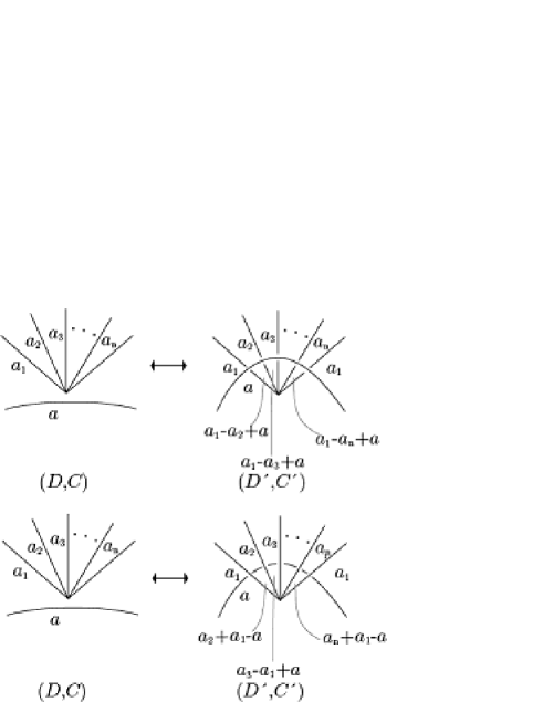
Figure 4.

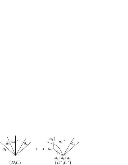
Figure 5.

Proposition 3.2 implies that the number of Dehn $p$-colorings, i.e. $\#{\rm Col}_{p}(D)$, is an invariant of spatial Euler graphs.

Remark 3.3.

For spatial graphs including an odd-valent vertex, even if we add any vertex condition, there does not exist a Dehn $p$-coloring such that $\#{\rm Col}_{p}(D)$ is an invariant of special graphs. This is because $\#{\rm Col}_{p}(D)$ might be changed under the Reidemeister move of type IV depicted in the lower picture of Figure 4.

4. Vertex-weight invariants of spatial Euler graphs

Let $f:U_{p}\to S$ be an invariant under the transformations (Op1)-(Op4) of Definition 1.1. For example, we can define $f$ under some proper situation by $f=\tau_{p}$, $f=\varepsilon_{p}$, $f=\mu_{p}$, $f=\mu_{p,\tau}$, $f=\tau_{p}\times\varepsilon_{p},\ldots,$ or $f=\tau_{p}\times\varepsilon_{p}\times\mu_{p}\times\mu_{p,\tau}$.

Let $D$ be a diagram of a spatial Euler graph $G$ and $C\in{\rm Col}_{p}(D)$. For a vertex $v$ of $D$ with regions $r_{1},r_{2},\ldots,r_{n}$ in clockwise direction as shown in Figure 6, we take a weight $W_{f}(D,C;v)$ as $W_{f}(D,C;v)=\Big{(}n,f\big{(}C(r_{1}),C(r_{2}),\ldots,C(r_{n})\big{)}\Big{)},$ where in this paper, we represent it by

$$W_{f}(D,C;v)=\Big{(}{\rm valency}=n,f=f\big{(}C(r_{1}),C(r_{2}),\ldots,C(r_{n})\big{)}\Big{)}$$

as an easy-to-understand way.

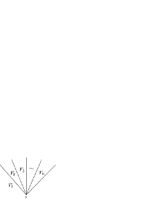
Figure 6.

We denote by $W_{f}(D,C)$ the multi-set of the weights of all vertices of $D$. As a multi-set, set

$$\Phi_{f}(D)=\Big{\{}W_{f}(D,C)~{}\Big{|}~{}C\in{\rm Col}_{p}(D)\Big{\}},$$

which we call the vertex-weight invariant of $D$ (or $G$) with respect to $f$. Then we have the following theorem:

Theorem 4.1.

Let $D$ and $D^{\prime}$ be diagrams of spatial Euler graphs. If $D$ and $D^{\prime}$ represent the same spatial graph, then we have $\Phi_{f}(D)=\Phi_{f}(D^{\prime})$. That is, $\Phi_{f}(D)$ is an invariant for spatial Euler graphs.

Proof.

First, we note that $W_{f}(D,C;v)$ does not depend on the starting region $r_{1}$ to read the regions $r_{1},\ldots,r_{n}$ in clockwise direction around $v$ since $f$ is unchanged under the transformation (Op1).

Now we show that $W_{f}(D,C;v)$ is unchanged under the Reidemeister moves of spatial graph diagrams. Let $D$ and $D^{\prime}$ be diagrams such that $D^{\prime}$ is obtained from $D$ by a single Reidemeister move shown in Figure 5. Let $C$ be a Dehn $p$-coloring of $D$, and $C^{\prime}$ the corresponding Dehn $p$-coloring of $D^{\prime}$. For an $n$-valent vertex $v$ of $(D,C)$ with $W_{f}(D,C;v)=\big{(}{\rm valency}=n,f=f(a_{1},a_{2},\ldots,a_{n})\big{)}$ as shown in the left of Figure 5, the corresponding vertex, say $v^{\prime}$, of $(D^{\prime},C^{\prime})$ has $W_{f}(D^{\prime},C^{\prime};v^{\prime})=\big{(}{\rm valency}=n,f=f(a_{1},-a_{1}+a_{2}+a_{3},a_{3},\ldots,a_{n})\big{)}$. Since $f$ is unchanged under the transformation (Op4) of Definition 1.1, we have $W_{f}(D^{\prime},C^{\prime};v^{\prime})=W_{f}(D,C;v)$. The same argument applies to the cases of the other Reidemeister moves. This implies that $W_{f}(D,C)=W_{f}(D^{\prime},C^{\prime})$, which leads to the property that $\Phi_{f}(D)=\Phi_{f}(D^{\prime})$. ∎

Remark 4.2.

We may arrange the definition of $W_{f}(D,C)$ for examples as follows: Define $W_{f}(D,C;v)$ by $W_{f}(D,C;v)=f\big{(}C(r_{1}),C(r_{2}),\ldots,C(r_{n})\big{)}$, and define $W_{f}(D,C)$ by the multiset of the weights of all vertices of $D$. In another way, define $W_{f}(D,C;v)$ by $W_{f}(D,C;v)=f\big{(}C(r_{1}),C(r_{2}),\ldots,C(r_{n})\big{)}$, and define $W_{f}(D,C)$ by the sum of the weights of all vertices of $D$ when the target set $S$ of $f$ has an Abelian group structure.

Example 4.3.

Let $G$ and $G^{\prime}$ be the spatial graphs depicted in Figure 7. The spatial graphs $G$ and $G^{\prime}$ can be distinguished with neither their constituent links nor $\#{\rm Col}_{p}$, and indeed, $\#{\rm Col}_{p}(G)=\#{\rm Col}_{p}(G^{\prime})=p^{5}$ holds for any $p\in\mathbb{Z}_{\geq 2}$. On the other hand, we can distinguish them with $\Phi_{\tau_{3}}$, which is shown as follows: We show that the multiset $\big{\{}({\rm valency}=4,\tau_{3}=1),({\rm valency}=6,\tau_{3}=3)\big{\}}$ is not included in $\Phi_{\tau_{3}}(G)$, while it is included in $\Phi_{\tau_{3}}(G^{\prime})$. For the diagram $D$, depicted in the left of Figure 8, of $G$ and a Dehn $3$-coloring $C\in{\rm Col}_{3}(D)$, assume that $W_{\tau_{3}}(D,C;v_{2})=3$ for the 6-valent vertex $v_{2}$. Then the regions $r_{1}$-$r_{6}$ around $v_{2}$ must be colored alternately as $C(r_{1})=a,C(r_{2})=b,C(r_{3})=a,C(r_{4})=b,C(r_{5})=a,C(r_{6})=b$ for some $a,b\in\mathbb{Z}_{3}$. Put $C(r_{7})=c$ for some $c\in\mathbb{Z}_{3}$. We then have $C(r_{8})=-a+b+c$, $C(r_{9})=2a-c$, $C(r_{10})=a+b-c$, $C(r_{11})=2a-c$ and $C(r_{12})=c$ from the crossing conditions at $c_{1}$, $c_{2}$, $c_{3}$, $c_{4}$ and $c_{5}$, respectively, in this order, see the right of Figure 8. Then the crossing condition at $c_{6}$ shows that

$$c=C(r_{12})=C(r_{9})-C(r_{8})+C(r_{10})=(2a-c)-(-a+b+c)+(a+b-c)=a,$$

which implies that the regions $r_{1}$, $r_{6}$, $r_{12}$, $r_{2}$ around $v_{1}$ must be colored alternately, that is, we have

$$W_{\tau_{3}}(D,C;v_{1})=\tau_{3}\big{(}C(r_{1}),C(r_{6}),C(r_{12}),C(r_{2})\big{)}=\tau_{3}(a,b,a,b)=3.$$

We note that the crossing condition at $c_{7}$ is satisfied when $a=c$. Therefore the multiset $\big{\{}({\rm valency}=4,\tau_{3}=1),({\rm valency}=6,\tau_{3}=3)\big{\}}$ is not included in $\Phi_{\tau_{3}}(G)$. On the other hand, the multiset $\big{\{}({\rm valency}=4,\tau_{3}=1),({\rm valency}=6,\tau_{3}=3)\big{\}}$ is included in $\Phi_{\tau_{3}}(G^{\prime})$ since the Dehn $3$-colored diagram of $G^{\prime}$ in Figure 9 gives this multiset.

Indeed, we have

$$\Phi_{\tau_{3}}(G)=\left.\begin{cases}\Big{\{}({\rm valency}=4,\tau_{3}=1),({\rm valency}=6,\tau_{3}=1)\Big{\}}(216{\rm times}),\\ \Big{\{}({\rm valency}=4,\tau_{3}=3),({\rm valency}=6,\tau_{3}=1)\Big{\}}(18{\rm times}),\\ \Big{\{}({\rm valency}=4,\tau_{3}=3),({\rm valency}=6,\tau_{3}=3)\Big{\}}(9{\rm times})\end{cases}\right\},$$

and

$$\Phi_{\tau_{3}}(G^{\prime})=\left.\begin{cases}\Big{\{}({\rm valency}=4,\tau_{3}=1),({\rm valency}=6,\tau_{3}=1)\Big{\}}(144{\rm times}),\\ \Big{\{}({\rm valency}=4,\tau_{3}=1),({\rm valency}=6,\tau_{3}=3)\Big{\}}(18{\rm times}),\\ \Big{\{}({\rm valency}=4,\tau_{3}=3),({\rm valency}=6,\tau_{3}=1)\Big{\}}(72{\rm times}),\\ \Big{\{}({\rm valency}=4,\tau_{3}=3),({\rm valency}=6,\tau_{3}=3)\Big{\}}(9{\rm times})\end{cases}\right\}.$$

Thus $G$ and $G^{\prime}$ can be distinguished by $\Phi_{\tau_{3}}$.

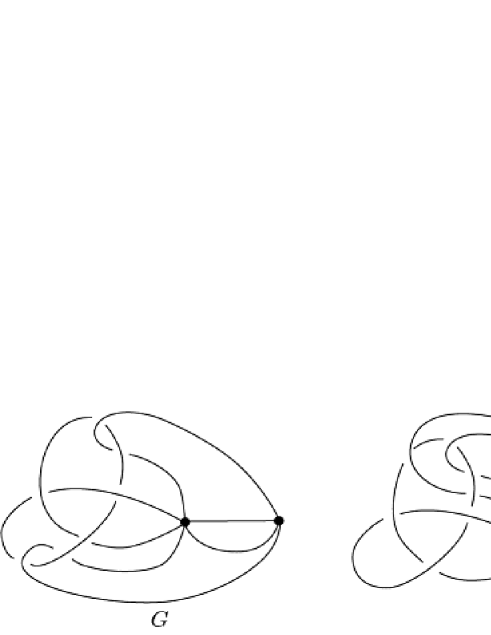
Figure 7.

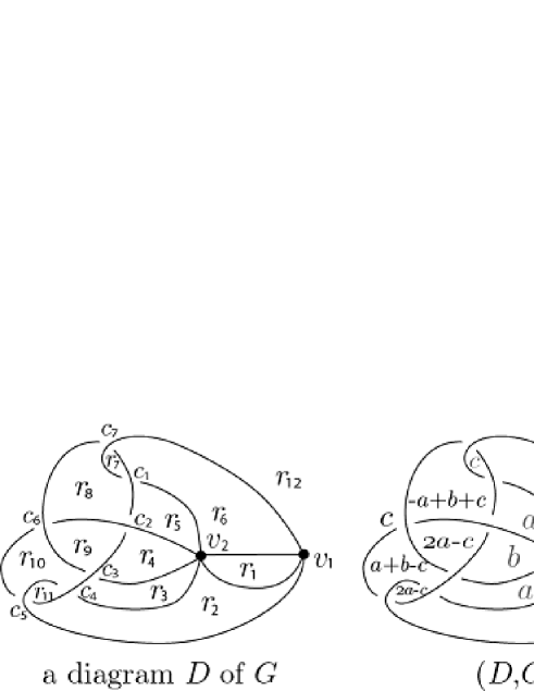
Figure 8.

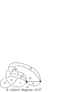
Figure 9.

Remark 4.4.

As mentioned in Remark 3.3, for spatial graphs including an odd-valent vertex, even if we add any vertex condition, there does not exist a vertex-weight invariant such that $\Phi_{f}(D)$ is an invariant of special graphs. This is because $\Phi_{f}(D)$ might be changed under the Reidemeister move of type IV depicted in the lower picture of Figure 4.

5. An application for spatial graphs with odd-valent vertices

In Section 3, we introduced the coloring invariants $\#{\rm Col}_{p}(G)$ of spatial Euler graphs, and in Section 4, we introduced the invariants $\Phi_{f}(G)$ of spatial Euler graphs. As mentioned in Remarks 3.3 and 4.4, for spatial graphs including odd-valent vertices, these invariants are meaningless. However, for spatial graphs with odd-valent vertices, we can apply our invariants to the spatial Euler graphs obtained by taking the parallel of some edges, and thus, our invariants can be also useful for spatial graphs with odd-valent vertices, where this method was introduced in [3]. In this section, we show how to apply our invariants to spatial graphs with odd-valent vertices in detail, and give some calculation example.

Let $G$ be a spatial graph and $E_{G}=\{e_{1},\ldots e_{s}\}$ the set of edges of $G$. We replace $r$ edges $e_{i_{1}},\ldots,e_{i_{r}}\in E_{G}$ without duplicates with the doubles of the edges, respectively, where the double of an edge $e$ is obtained by replacing the edge $e$ with the $2$-parallel $e_{+}\cup e_{-}$ of $e$ such that $e_{+}$ and $e_{-}$ are connected at the end points of $e$ as in Figure 10. Here one might think that there is an ambiguity for twists of the parallel edges $e_{+}$ and $e_{-}$, and however, the ambiguity can be solved by equivalence transformations of spatial graphs corresponding to the Reidemeister moves of type V.

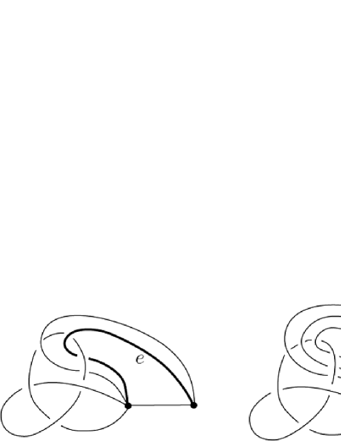
Figure 10.

We call the resultant spatial graph the double of $G$ with respect to $\{e_{i_{1}},\ldots,e_{i_{r}}\}$, and we denote it by $d(G;\{e_{i_{1}},\ldots,e_{i_{r}}\})$. We say that $\{e_{i_{1}},\ldots,e_{i_{r}}\}$ is doublable if $d(G;\{e_{i_{1}},\ldots,e_{i_{r}}\})$ is a spatial Euler graph. For $r\in\mathbb{Z}_{+}$, we set

$$d{\rm Edges}(G;r)=\left\{\{e_{i_{1}},\ldots,e_{i_{r}}\}\subset E_{G}~{}\Big{|}~{}\begin{array}[]{l}\{e_{i_{1}},\ldots,e_{i_{r}}\}\mbox{ is doublable, and}\\ \#\{e_{i_{1}},\ldots,e_{i_{r}}\}=r\end{array}\right\}.$$

Let $\Phi$ be an invariant of spatial Euler graphs. For a spatial graph $G$ that might have an odd-valent vertex and $r\in\mathbb{Z}_{+}$, set

$$\Phi(G;r)=\big{\{}\Phi\big{(}d(G;\{e_{i_{1}},\ldots,e_{i_{r}}\})\big{)}~{}\big{|}~{}\{e_{i_{1}},\ldots,e_{i_{r}}\}\in d{\rm Edges}(G;r)\big{\}}$$

as a multiset. We have the following proposition:

Proposition 5.1.

$\Phi(G;r)$ is an invariant of spatial graphs.

Proof.

Put

$$d(G;r)=\big{\{}d(G;\{e_{i_{1}},\ldots,e_{i_{r}}\})~{}\big{|}~{}\{e_{i_{1}},\ldots,e_{i_{r}}\}\in d{\rm Edges}(G;r)\big{\}}.$$

We then have that if two spatial graphs $G_{1}$ and $G_{2}$ are equivalent, then there exists a bijection $\psi:d(G_{1};r)\to d(G_{2};r)$ such that for $G_{1}^{\prime}\in d(G_{1};r)$ and $G_{2}^{\prime}=\psi(G_{1}^{\prime})$, $G_{1}^{\prime}$ and $G_{2}^{\prime}$ are equivalent, see [3]. Besides, by Theorem 4.1, we have $\Phi(G_{1}^{\prime})=\Phi(G_{2}^{\prime})$. This completes the proof. ∎

Example 5.2.

Let $G_{1}$ and $G_{2}$ be the spatial graphs depicted in Figure 11. We note that they have odd-valent vertices. Let us consider the case that $\Phi=\Phi_{\tau_{3}}$ and $r=1$ for $\Phi(G_{1};r)$ and $\Phi(G_{2};r)$. Since $d{\rm Edges}(G_{1};1)=\big{\{}\{e_{11}\},\{e_{12}\},\{e_{13}\}\big{\}}$ and $d{\rm Edges}(G_{2};1)=\big{\{}\{e_{21}\},\{e_{22}\},\{e_{23}\}\big{\}}$ as depicted in Figure 11,

$$\Phi_{\tau_{3}}(G_{1};1)=\big{\{}\Phi_{\tau_{3}}\big{(}d(G_{1};\{e_{11}\})\big{)},\Phi_{\tau_{3}}\big{(}d(G_{1};\{e_{12}\})\big{)},\Phi_{\tau_{3}}\big{(}d(G_{1};\{e_{13}\})\big{)}\big{\}},\mbox{ and }$$

$$\Phi_{\tau_{3}}(G_{2};1)=\big{\{}\Phi_{\tau_{3}}\big{(}d(G_{2};\{e_{21}\})\big{)},\Phi_{\tau_{3}}\big{(}d(G_{2};\{e_{22}\})\big{)},\Phi_{\tau_{3}}\big{(}d(G_{2};\{e_{23}\})\big{)}\big{\}},$$

see Figures 12 and 13. Since we have

$$\big{\{}\Phi_{\tau_{3}}\big{(}d(G_{1};\{e_{11}\})\big{)},\Phi_{\tau_{3}}\big{(}d(G_{1};\{e_{12}\})\big{)},\Phi_{\tau_{3}}\big{(}d(G_{1};\{e_{13}\})\big{)}\big{\}}=\big{\{}\mathbb{A},\mathbb{A},\mathbb{A}\big{\}}$$

and

$$\big{\{}\Phi_{\tau_{3}}\big{(}d(G_{2};\{e_{21}\})\big{)},\Phi_{\tau_{3}}\big{(}d(G_{2};\{e_{22}\})\big{)},\Phi_{\tau_{3}}\big{(}d(G_{2};\{e_{23}\})\big{)}\big{\}}=\big{\{}\mathbb{A},\mathbb{A},\mathbb{B}\big{\}},$$

it holds that $\Phi_{\tau_{3}}(G_{1};1)\not=\Phi_{\tau_{3}}(G_{2};1)$, where

$$\mathbb{A}=\left.\begin{cases}\Big{\{}({\rm valency}=4,\tau_{3}=1),({\rm valency}=6,\tau_{3}=1)\Big{\}}(216{\rm times}),\\ \Big{\{}({\rm valency}=4,\tau_{3}=3),({\rm valency}=6,\tau_{3}=1)\Big{\}}(18{\rm times}),\\ \Big{\{}({\rm valency}=4,\tau_{3}=3),({\rm valency}=6,\tau_{3}=3)\Big{\}}(9{\rm times})\end{cases}\right\}$$

and

$$\mathbb{B}=\left.\begin{cases}\Big{\{}({\rm valency}=4,\tau_{3}=1),({\rm valency}=6,\tau_{3}=1)\Big{\}}(144{\rm times}),\\ \Big{\{}({\rm valency}=4,\tau_{3}=1),({\rm valency}=6,\tau_{3}=3)\Big{\}}(18{\rm times}),\\ \Big{\{}({\rm valency}=4,\tau_{3}=3),({\rm valency}=6,\tau_{3}=1)\Big{\}}(72{\rm times}),\\ \Big{\{}({\rm valency}=4,\tau_{3}=3),({\rm valency}=6,\tau_{3}=3)\Big{\}}(9{\rm times})\end{cases}\right\}.$$

Thus $G_{1}$ and $G_{2}$ can be distinguished by $\Phi_{\tau_{3}}(\,\bullet\,;1)$. We note that $G_{1}$ and $G_{2}$ can be distinguished by neither their constituent links nor the coloring numbers $\#{\rm Col}_{p}(\,\bullet\,;1)$ for any $p\in\mathbb{Z}_{\geq 2}$, where $\#{\rm Col}_{p}(G_{1};1)=\#{\rm Col}_{p}(G_{2};1)=\{p^{5},p^{5},p^{5}\}$.

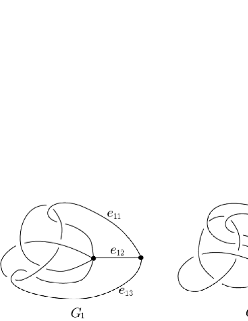
Figure 11.

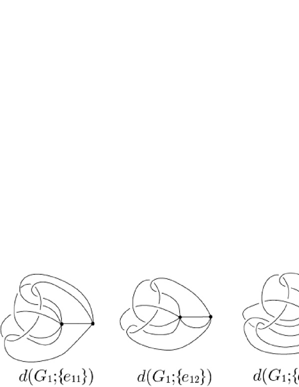
Figure 12.

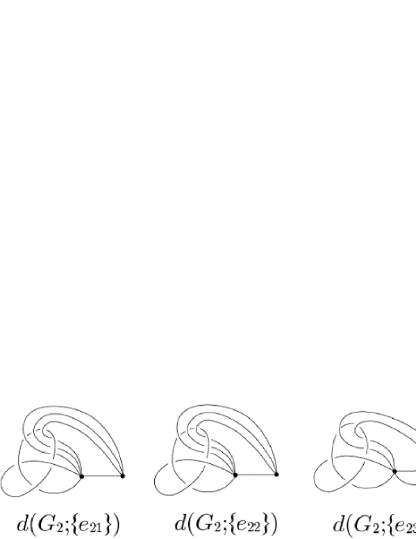
Figure 13.

References

- [1] J. S. Carter, D. S. Silver, and S. G. Williams, Three dimensions of knot coloring, Amer. Math. Monthly 121 (2014), no. 6, 506–514.
- [2] F. Harary and L. H. Kauffman, Knots and graphs I. Arc graphs and colorings, Adv. in Appl. Math. 22 (3) (1999) 312–337.
- [3] Y. Ishii and A. Yasuhara, Color invariant for spatial graphs, J. Knot Theory Ramifications 6 (1997), no. 3, 319–325.
- [4] D. Joyce, A classifying invariant of knots, the knot quandle, J. Pure Appl. Algebra 23 (1982), no. 1, 37–65.
- [5] A. Madaus, M. Newman, and H. M. Russell, Dehn coloring and the dimer model for knots, J. Knot Theory Ramifications 26 (2017), no. 3, 1741008, 18 pp.
- [6] S. V. Matveev, Distributive groupoids in knot theory, Mat. Sb. (N.S.) 119( 161) (1982), no. 1, 78–88, 160.
- [7] M. Niebrzydowski, On some ternary operations in knot theory, Fund. Math. 225 (2014), no. 1, 259–276.
- [8] K. Oshiro, On pallets for Fox colorings of spatial graphs, Topology Appl. 159 (2012), no. 4, 1092–1105.
- [9] K. Oshiro and N. Oyamaguchi, Palettes of Dehn colorings for spatial graphs and the classification of vertex conditions, preprint.
- [10] J. Przytycki, -coloring and other elementary invariants of knots, Knot theory (Warsaw, 1995), 275–295, Banach Center Publ. 42, Polish Acad. Sci. Inst. Math., Warsaw, 1998.
- [11] S. Satoh, A note on the shadow cocycle invariant of a knot with a base point, J. Knot Theory Ramifications 16 (2007), no. 7, 959–967.