Steered quantum coherence as a signature of quantum phase transitions in spin chains

Abstract

We propose to use the steered quantum coherence (SQC) as a signature of quantum phase transitions (QPTs). By considering various spin chain models, including the transverse-field Ising model, XY model, and XX model with three-spin interaction, we showed that the SQC and its first-order derivative succeed in signaling different critical points of QPTs. In particular, the SQC method is effective for any spin pair chosen from the chain, and the strength of SQC, in contrast to entanglement and quantum discord, is insensitive to the distance (provided it is not very short) of the tested spins, which makes it convenient for practical use as there is no need for careful choice of two spins in the chain.

I Introduction

Quantum coherence plays a fundamental role in the fields of quantum optics Ficek and thermodynamics ther5 . The resource theoretic framework for quantifying coherence formulated in 2014 stimulates further study of it from a quantitative perspective coher ; Plenio ; Hu . In particular, it has been used to explain the quantum advantage of many emerging quantum computation tasks, including quantum state merging qsm , deterministic quantum computation with one qubit DQC1 , Deutsch-Jozsa algorithm DJ , and Grover search algorithm Grover . The resource theory of coherence also provides a basis for interpreting the wave nature of a quantum system path1 ; path2 and the essence of quantum correlations such as quantum entanglement coher-ent ; convex3 ; SQC ; naqc2 ; naqc3 ; Tan and various discordlike quantum correlations DQC1 ; Tan ; Yao ; Hufan ; Hux1 ; Yuc ; Hux2 .

Besides the fundamental position in physics, quantum coherence is also useful in studying critical behaviors of various spin chain systems. For instance, the relative entropy of coherence for one spin or two adjacent spins can detect quantum phase transitions (QPTs) in the spin-1/2 transverse-field Ising, XX, and Kitaev honeycomb models chenj , while critical behaviors of the XY model have been studied by virtue of the $l_{1}$ norm of coherence Qin . Moreover, the relative entropy and $l_{1}$ norm of coherence for two neighboring spins detect successfully the Ising-type first-order QPT in the spin-1 XXZ model spin1 . The skew-information-based coherence measure skif , though it is not well defined Dubai , can also detect QPTs in certain spin chain models, including the spin-1/2 XY model either without Karpat or with three-spin interaction Leisg ; Liyc and the spin-1/2 XYZ model with Dzyaloshinsky-Moriya interaction Ywl .

In fact, other characterizations of quantumness in quantum information science have also been used to study QPTs. One of them is entanglement EoF . Its role in exploring QPTs can be found in Refs. nature ; Osborne ; Gusj1 ; Gusj2 and the review work Amico . Another quantumness measure is entropic quantum discord QD ; QD2 , which can detect QPTs in the XXZ model XXZ ; Sarandy , the transverse-field Ising model Ising ; Sarandy , the transverse-field XY model XY , and the XY model with three-spin XYthree or Dzyaloshinsky-Moriya interaction XYDM . Moreover, one can also use geometric quantum discord to explore QPTs in certain spin chain models Hu . Nevertheless, although entanglement and quantum discord were widely used to explore QPTs with great success, entanglement is short ranged Amico , so a careful choice of two very short distance spins or the bipartition of the system is required. Quantum discord, though can exist for two relatively long-distance spins, its computation is NP complete qd-np (there is no closed formula even for a general two-qubit state qdtwo ). These limit the scope of their applications in exploring QPTs.

In this paper, we propose to use the steered quantum coherence (SQC) SQC as a signature of QPTs. We consider a general XY model with a transverse magnetic field and three-spin interaction, and show that the SQC precisely signals all critical points of the QPTs. In particular, compared with entanglement and quantum discord, the SQC exists for any two spins in the chain, and its strength is insensitive to the distance of two spins provided it is not very short. This remarkable property of SQC releases the restriction on the distance of the spin pair selected for probing QPTs and may have important implications for experimental observation of QPTs as, in general, it is hard to measure a weak quantity in experiments. Moreover, different from quantum coherence of a state which is basis dependent and one may extract useless information if the basis is inappropriate, the SQC is analytically solvable for any two-spin state and its value is definite. On the experimental side, the SQC can be estimated by local projective measurements and one-qubit tomography, which is also feasible with current techniques qcexp1 ; qcexp2 ; qcexp3 . All the aspects above show that the SQC may be a powerful tool to study QPTs in spin chain models.

The structure of this paper is as follows. In Sec. II, we recall definition of the SQC and solution of the physical model. Then in Sec. III, we discuss critical behaviors of SQC for the considered model and show that it signals the QPTs precisely. Finally, we summarize our main finding in Sec. IV.

II Preliminaries

We first present definition of the SQC. For a state $\rho_{AB}$ with the two qubits held, respectively, by Alice and Bob, the SQC was defined by Alice’s local measurements and classical communication between Alice and Bob. To be explicit, Alice carries out one of the pre-agreed measurements $\{\sigma^{\mu}\}_{\mu=x,y,z}$ ($\sigma^{\mu}$ is the Pauli operator) on qubit $A$ and communicates to Bob her choice $\sigma^{\mu}$. Then Bob’s system collapses to the ensemble states $\{p_{\mu,a},\rho_{B|\Pi_{\mu}^{a}}\}$, with $p_{\mu,a}=\mathrm{tr}(\Pi_{\mu}^{a}\rho_{AB})$ being the probability of Alice’s outcome $a\in\{0,1\}$, and $\rho_{B|\Pi_{\mu}^{a}}=\mathrm{tr}_{A}(\Pi_{\mu}^{a}\rho_{AB})/p_{\mu,a}$ being Bob’s conditional state. Moreover, $\Pi_{\mu}^{a}=[\openone_{2}+(-1)^{a}\sigma^{\mu}]/2$ is the measurement operator and $\openone_{2}$ is the identity operator.

For Alice’s chosen observable $\sigma^{\mu}$, Bob can measure the coherence of the ensemble $\{p_{\mu,a},\rho_{B|\Pi_{\mu}^{a}}\}$ with respect to the eigenbasis of either one of the remaining two Pauli operators. After Alice’s all possible measurements $\{\Pi_{\mu}^{a}\}_{\mu=x,y,z}$ with equal probability, the SQC at Bob’s hand can be defined as the following averaged quantum coherence SQC

$$C^{na}(\rho_{AB})=\frac{1}{2}\sum_{\mu,\nu,a\atop\mu\neq\nu}p_{\mu,a}C^{\sigma^{\nu}}(\rho_{B|\Pi_{\mu}^{a}}),$$ (1)

where $C^{\sigma^{\nu}}(\rho_{B|\Pi_{\mu}^{a}})$ is the coherence of $\rho_{B|\Pi_{\mu}^{a}}$ defined in the reference basis spanned by the eigenbases of $\sigma^{\nu}$ coher .

In this paper, we use the $l_{1}$ norm of coherence and the relative entropy of coherence which are favored for their ease of calculation. By denoting $\{|\psi_{i}\rangle\}$ the eigenbases of $\sigma^{\nu}$, their analytical solutions are given, respectively, by coher

$$\begin{split}&C_{l_{1}}^{\sigma^{\nu}}(\rho)=\sum_{i\neq j}|\langle\psi_{i}|\rho|\psi_{j}\rangle|,\\ &C_{re}^{\sigma^{\nu}}(\rho)=-\sum_{i}\langle\psi_{i}|\rho|\psi_{i}\rangle\log_{2}\langle\psi_{i}|\rho|\psi_{i}\rangle-S(\rho),\end{split}$$ (2)

with $S(\rho)=-\mathrm{tr}(\rho\log_{2}\rho)$ denoting the von Neumann entropy. Based on these formulas, one can then obtain the corresponding SQC $C_{l_{1}}^{na}(\rho_{AB})$ and $C_{re}^{na}(\rho_{AB})$.

Next, we introduce the XY model with a transverse magnetic field and three-spin interaction. The Hamiltonian for such a model can be written as

$$\begin{split}\hat{H}=&-\sum\limits_{n=1}^{N}\left(\frac{1+\gamma}{2}{\sigma_{n}^{x}\sigma_{n+1}^{x}}+\frac{1-\gamma}{2}{\sigma_{n}^{y}\sigma_{n+1}^{y}}+\lambda\sigma_{n}^{z}\right)\\ &-\sum\limits_{n=1}^{N}\alpha({\sigma_{n-1}^{x}\sigma_{n}^{z}\sigma_{n+1}^{x}}+{\sigma_{n-1}^{y}\sigma_{n}^{z}\sigma_{n+1}^{y}}),\end{split}$$ (3)

where $\sigma_{n}^{\mu}$ ($\mu=x,y,z$) are the Pauli operators at site $n$, $\lambda$ is the transverse magnetic field, $\gamma$ denotes the anisotropy of the system arising from the nearest-neighbor interaction, and $\alpha$ denotes the strength of the three-spin interaction arising from the next-to-nearest-neighbor interaction three . Moreover, $N$ is the number of spins in the chain, and we assume the periodic boundary conditions.

The Hamiltonian $\hat{H}$ can be diagonalized by first using the Jordan-Wigner transformation QPTs2

$$\begin{split}&\sigma_{n}^{x}=\prod_{m<n}\left(1-2{c_{m}^{\dagger}}c_{m}\right)\left(c_{n}+c_{n}^{\dagger}\right),\\ &\sigma_{n}^{y}=-i\prod_{m<n}\left(1-2{c_{m}^{\dagger}}c_{m}\right)\left(c_{n}-c_{n}^{\dagger}\right),~{}\sigma_{n}^{z}=1-2c_{n}^{\dagger}c_{n},\end{split}$$ (4)

which maps the spins to spinless fermions with the creation (annihilation) operators $c_{n}^{\dagger}$ ($c_{n}$). Then by virtue of the Fourier transformation $\tilde{c}_{k}=\sum_{l}c_{l}e^{-ilx_{k}}/\sqrt{N}$ ($x_{k}=2\pi k/N$) and the Bogoliubov transformation $d_{k}=\cos(\theta_{k}/2)\tilde{c}_{k}-i\sin(\theta_{k}/2)\tilde{c}_{-k}^{\dagger}$, one can obtain epjb

$$\hat{H}=\sum_{k=-M}^{M}2\varepsilon_{k}\left(d_{k}^{\dagger}d_{k}-\frac{1}{2}\right),$$ (5)

where $M=(N-1)/2$, $\theta_{k}=\arcsin[-\gamma\sin(x_{k})/\varepsilon_{k}]$, and the energy spectrum is given by

$$\varepsilon_{k}=\sqrt{\epsilon_{k}^{2}+\gamma^{2}\sin^{2}(x_{k})},$$ (6)

with $\epsilon_{k}=\lambda-\cos(x_{k})-2\alpha\cos(2x_{k})$.

To calculate the SQC, one needs to obtain the density operator $\rho_{i,i+r}$ for the spin pair $(i,i+r)$, with $r$ denoting the distance of two spins in units of the lattice constant. In the Bloch representation, $\rho_{i,i+r}$ can always be decomposed as

$$\rho_{i,i+r}=\frac{1}{4}\sum_{\mu,\nu}t_{\mu\nu}\sigma_{i}^{\mu}\otimes\sigma_{i+r}^{\nu},$$ (7)

where $\mu,\nu\in\{0,x,y,z\}$, $t_{\mu\nu}=\mathrm{tr}(\rho_{i,i+r}\sigma_{i}^{\mu}\otimes\sigma_{i+r}^{\nu})$, and $\sigma_{i}^{0}=\openone_{2}$. Due to the translation invariance, $\rho_{i,i+r}$ will be independent of the position $i$ and depends only on the distance $r$ of two spins. Then one can obtain the nonzero $t_{\mu\nu}$ of $\rho_{i,i+r}$ as Wang ; Gusj

$$t_{z0}=t_{0z}=\langle\sigma^{z}\rangle,~{}t_{\mu\mu}=\langle\sigma_{i}^{\mu}\sigma_{i+r}^{\mu}\rangle~{}(\mu\in\{x,y,z\}),$$ (8)

where $\langle\sigma^{z}\rangle$ is the magnetization intensity given by magnet

$$\langle\sigma^{z}\rangle=\frac{1}{N}\sum_{k}\frac{\epsilon_{k}\tanh(\beta\varepsilon_{k})}{\varepsilon_{k}},$$ (9)

and $\beta=1/k_{B}T$, with $k_{B}$ being the Boltzmann constant. Moreover, the spin-spin correlation functions are given by xyt1

$$\begin{split}\langle\sigma_{i}^{x}\sigma_{i+r}^{x}\rangle&=\begin{vmatrix}G_{-1}&G_{-2}&\cdots&G_{-r}\\ G_{0}&G_{-1}&\cdots&G_{-r+1}\\ \vdots&\vdots&\ddots&\vdots\\ G_{r-2}&G_{r-3}&\cdots&G_{-1}\end{vmatrix},\\ \langle\sigma_{i}^{y}\sigma_{i+r}^{y}\rangle&=\begin{vmatrix}G_{1}&G_{0}&\cdots&G_{-r+2}\\ G_{2}&G_{1}&\cdots&G_{-r+3}\\ \vdots&\vdots&\ddots&\vdots\\ G_{r}&G_{r-1}&\cdots&G_{1}\end{vmatrix},\end{split}$$ (10)

and $\langle\sigma_{i}^{z}\sigma_{i+r}^{z}\rangle={\langle\sigma_{i}^{z}\rangle}^{2}-G_{r}G_{-r}$, where $G_{n}$ ($-r\leqslant n\leqslant r$) is given by

$$G_{n}=-\sum_{k}\frac{[\cos(nx_{k})\epsilon_{k}+\gamma\sin(nx_{k})\sin(x_{k})]\tanh\left(\beta\varepsilon_{k}\right)}{N\varepsilon_{k}}.$$ (11)

For the two-spin density operator $\rho_{i,i+r}$ with its nonzero elements constrained by Eq. (8), the SQC can be obtained analytically as

$$\begin{aligned} C_{l_{1}}^{na}(\rho_{i,i+r})=&t_{0z}+\frac{1}{2}\left(t_{xx}+t_{yy}+\sqrt{t_{0z}^{2}+t_{xx}^{2}}+\sqrt{t_{0z}^{2}+t_{yy}^{2}}\right),\\ C_{re}^{na}(\rho_{i,i+r})=&2-H_{2}(\tau_{1})-H_{2}(\tau_{2})-\frac{(1+t_{z0})H_{2}(\tau_{3})}{2}\\ &-\frac{(1-t_{z0})H_{2}(\tau_{4})}{2}+H_{2}\left(\frac{1+t_{0z}}{2}\right),\end{aligned}$$ (12)

where $H_{2}(\cdot)$ denotes the binary Shannon entropy function, and the parameters $\tau_{i}$ ($i=1,2,3,4$) are given by

$$\tau_{1}=\frac{1}{2}\left(1+\sqrt{t_{0z}^{2}+t_{xx}^{2}}\right),~{}\tau_{2}=\frac{1}{2}\left(1+\sqrt{t_{0z}^{2}+t_{yy}^{2}}\right),$$ (13)

$$\tau_{3}=\frac{1}{2}+\frac{|t_{0z}+t_{zz}|}{2(1+t_{z0})},~{}\tau_{4}=\frac{1}{2}+\frac{|t_{0z}-t_{zz}|}{2(1-t_{z0})}.$$

III SQC and QPTs in spin chain models

Based on the above preliminaries, we discuss in this section critical behaviors of the spin chain described by Eq. (3) by using the SQC. We show that the extreme points of the SQC for any two spins as well as the discontinuity of its first derivative are able to indicate QPTs in the considered model.

III.1 Transverse-field Ising model

To begin with, we consider the transverse-field Ising model which corresponds to $\gamma=1$ and $\alpha=0$ in Eq. (3). For such a model, it is known that there is a second-order QPT at $\lambda_{c}=1$. At this point, the global phase flip symmetry breaks and the correlation length diverges Amico .

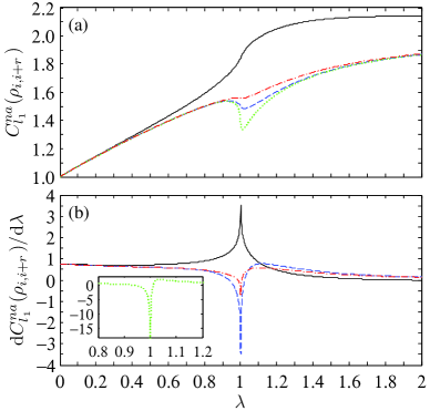
Figure 1: $C_{l_{1}}^{na}(\rho_{i,i+r})$ (a) and its first derivative $\mathrm{d}C_{l_{1}}^{na}(\rho_{i,i+r})/\mathrm{d}\lambda$ (b) versus $\lambda$ for the Ising model with $N=2001$. The solid black, dash-dotted red, dashed blue, and dotted green lines correspond to $r=1$, 5, 10, and 100, respectively. The dotted green line in panel (b) is shown in the inset to better visual the QPT.

To reveal that the SQC can indicate QPTs in the Ising model, we show in Fig. 1 the dependence of $C_{l_{1}}^{na}(\rho_{i,i+r})$ and its first derivative on $\lambda$ with different distances $r$ of the spin pair. For $r\leqslant 3$, $C_{l_{1}}^{na}(\rho_{i,i+r})$ increases monotonically with the increase of $\lambda$, and its first-order derivative with respect to $\lambda$ shows a discontinuity at $\lambda_{c}=1$. For the tested spins with long distances ($r\geqslant 4$), as depicted in Fig. 1(a), $C_{l_{1}}^{na}(\rho_{i,i+r})$ does not behave as a monotonic increasing function of $\lambda$. Instead, there exists a pronounced cusp close to $\lambda_{c}=1$. A further numerical calculation shows that the critical point $\lambda_{t}$ for the minimum of this cusp approaches monotonically to $\lambda_{c}$ with the increase of $r$, e.g., $\lambda_{t}-\lambda_{c}\sim 10^{-6}$ when $r=1000$ and $N=2001$. Then it is reasonable to conclude that for an infinite chain, the minimum of this cusp can precisely signal the QPT at $\lambda_{c}=1$ when $r$ is very large. Moreover, one can observe from Fig. 1(b) that the discontinuity of $\mathrm{d}C_{l_{1}}^{na}(\rho_{i,i+r})/\mathrm{d}\lambda$ indicates the QPT at $\lambda_{c}=1$ for the chosen tested spins with any distance.

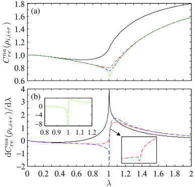
Figure 2: $C_{re}^{na}(\rho_{i,i+r})$ (a) and its first derivative $\mathrm{d}C_{re}^{na}(\rho_{i,i+r})/\mathrm{d}\lambda$ (b) versus $\lambda$ for the Ising model with $N=2001$. The solid black, dash-dotted red, dashed blue, and dotted green lines correspond to $r=1$, 5, 10, and 100, respectively. The inset in the bottom right corner is an amplified plot of the dash-dotted red line in the neighborhood of $\lambda_{c}$, and the dotted green line in panel (b) is shown in the top left corner to better visual the QPT.

With the same system parameters as in Fig. 1, we displayed in Fig. 2 dependence of $C_{re}^{na}(\rho_{i,i+r})$ and its first derivative on $\lambda$. One can see that with the increasing strength of the transverse magnetic field $\lambda$, $C_{re}^{na}(\rho_{i,i+r})$ first decreases to a minimum, and then turns to be increased gradually. As for $\rho_{i,i+r}$ with large $r$, $C_{re}^{na}(\rho_{i,i+r})$ also shows a pronounced cusp in the neighborhood of $\lambda_{c}$, and with the increase of $r$, the critical point of $\lambda_{t}$ for the minimum of this cusp approaches to $\lambda_{c}$ more rapidly than that for $C_{l_{1}}^{na}(\rho_{i,i+r})$, e.g., $\lambda_{t}-\lambda_{c}\sim 10^{-8}$ for $r=1000$ and $N=2001$. This suggests that the cusp of SQC can signal the QPT taking place at $\lambda_{c}$ for two long-distance tested spins. Moreover, the first-order derivative of $C_{re}^{na}(\rho_{i,i+r})$, as expected, also presents a discontinuity at the phase transition point $\lambda_{c}=1$ for two spins with different distances.

All the above observations show evidently that the SQC and its first-order derivative for any two spins can clearly indicate QPT in the Ising model. In particular, one can see from Figs. 1 and 2 that beyond the adjacent region of $\lambda_{c}$, the curves of SQC for two spins with different large $r$ are nearly overlapped; i.e., there is almost no decrease of the SQC for $\rho_{i,i+r}$ with different large $r$. Such a property can be immediately applied to reduce the experimental demands to detect QPTs, as one can choose two spins at any distance to achieve the same feat.

We have also checked efficiency of other signatures of QPT. For entanglement and quantum discord, the discontinuities of their first derivatives can detect QPTs in the Ising chain Ising . But the entanglement exists only for $r\leqslant 2$, and hence imposes a strict restriction on the distance of the tested spins, while the calculation of quantum discord is a hard task even when $\rho_{i,i+r}$ is available qdtwo . Moreover, it can be seen from Eqs. (7) and (8) that the one-spin coherence is always zero. As for the two-spin coherence, its derivative shows a discontinuity at $\lambda_{c}$, but its estimation needs a two-qubit state tomography.

III.2 Transverse-field XY model

Next, we consider the transverse-field XY model, which corresponds to $\alpha=0$ in Eq. (3). There are two QPTs phase ; QPTxy . The first one occurs at $\lambda_{c}=1$. For $\lambda<\lambda_{c}$, the system is in the ferromagnetic ordered phase, while for $\lambda>\lambda_{c}$ it is in the paramagnetic quantum disordered phase. The second one occurs at $\gamma_{c}=0$ and $\lambda\in(0,1)$. It further separates the ferromagnetic ordered phase into two regions, i.e., the ferromagnet ordered along either the $x$ ($\gamma<0$) or the $y$ ($\gamma>0$) axis.

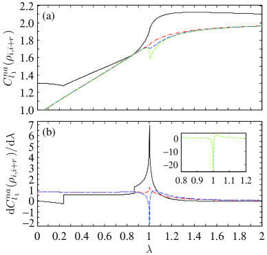
Figure 3: $C_{l_{1}}^{na}(\rho_{i,i+r})$ (a) and its first derivative $\mathrm{d}C_{l_{1}}^{na}(\rho_{i,i+r})/\mathrm{d}\lambda$ (b) versus $\lambda$ for the XY model with $\gamma=0.5$ and $N=2001$. The solid black, dash-dotted red, dashed blue, and dotted green lines correspond to $r=1$, 5, 10, and 100, respectively. The dotted green line in panel (b) is shown in the inset to better visual the QPT.

In Fig. 3, we show the dependence of $C_{l_{1}}^{na}(\rho_{i,i+r})$ and its first derivative on $\lambda$ for the XY model with $\gamma=0.5$. For two neighboring spins, the discontinuity of $\mathrm{d}C_{l_{1}}^{na}(\rho_{i,i+r})/\mathrm{d}\lambda$ precisely signals the QPT at $\lambda_{c}$, and there exist two inflexions for it, which are not critical points of QPTs xyt1 ; xyt2 . When $r$ is large, the curves of $C_{l_{1}}^{na}(\rho_{i,i+r})$ with different $r$ are nearly overlapped beyond the adjacent region of $\lambda_{c}$, and there exists an abrupt cusp in the neighborhood of $\lambda_{c}$. The critical point of $\lambda_{t}$ corresponds to the minimum of this cusp approaches asymptotically to $\lambda_{c}$ with the increase of $r$, e.g., $\lambda_{t}-\lambda_{c}\sim 10^{-7}$ when $r=1000$ and $N=2001$. Similar to the Ising model, the insensitivity of the SQC to the distance (provided it is not very short) of the tested spins in the XY chain also has important practical consequences for experimental characterization of QPTs. With regard to the first-order derivative of $C_{l_{1}}^{na}(\rho_{i,i+r})$, it shows a discontinuity at $\lambda_{c}$, irrespective of $r$. Hence, it is able to precisely detect the QPT for two spins at any distance.

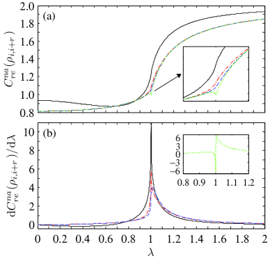
Figure 4: $C_{re}^{na}(\rho_{i,i+r})$ (a) and its first derivative $\mathrm{d}C_{re}^{na}(\rho_{i,i+r})/\mathrm{d}\lambda$ (b) versus $\lambda$ for the XY model with $\gamma=0.5$ and $N=2001$. The solid black, dash-dotted red, dashed blue, and dotted green lines correspond to $r=1$, 5, 10, and 100, respectively. The inset in panel (a) is an amplified plot of the lines in the neighborhood of $\lambda_{c}$, and the dotted green line in panel (b) is shown in the inset to better visual the QPT.

Similarly, we show in Fig. 4 the capability of $C_{re}^{na}(\rho_{i,i+r})$ and its derivative in detecting QPT at $\lambda_{c}=1$. First, for two spins with long distances, the curves of $C_{re}^{na}(\rho_{i,i+r})$ are nearly overlapped for $\lambda$ deviating from the adjacent region of $\lambda_{c}$. On the contrary, there is a cusp close to $\lambda_{c}$, and the critical $\lambda_{t}$ related to the bottom of this cusp approaches rapidly to $\lambda_{c}$ with the increase of $r$, e.g., $\lambda_{t}-\lambda_{c}\sim 10^{-10}$ when $r=1000$ and $N=2001$. Second, the first derivative of $C_{re}^{na}(\rho_{i,i+r})$ shows a discontinuity at $\lambda_{c}$, irrespective of the distance of the spin pair in the chain. This indicates that the phase transition point in the XY model can also be signaled precisely by $\mathrm{d}C_{re}^{na}(\rho_{i,i+r})/\mathrm{d}\lambda$.

We have also examined QPTs of the XY model at $\gamma_{c}=0$ and $\lambda\in(0,1)$. For conciseness of this paper, we do not present the plots here. The numerical calculation shows that this QPT can be signaled precisely by the extremal behaviors of the SQC. To be explicit, $C_{l_{1}}^{na}(\rho_{i,i+r})$ is maximal for $r=1$ and minimal for $r\geqslant 2$ at $\gamma_{c}$, while $C_{re}^{na}(\rho_{i,i+r})$ always reaches to its minimum at $\gamma_{c}$. However, there is no extremal, discontinuous, or singular behavior being observed for the first-order derivative of the SQC with respect to the anisotropic parameter $\gamma$.

As for concurrence of $\rho_{i,i+r}$, it is non-null for two spins with very short distance; e.g., for $\gamma=0.5$, its first derivative detects the QPT at $\lambda_{c}$ only when $r\leqslant 3$. The critical point $\lambda_{c}$ can also be detected by the first derivative of quantum discord for two spins more distant than second neighbors XY , and similarly for the two-spin coherence. However, the strength of quantum discord and two-spin coherence decrease as we increase $r$, especially in the region of $\lambda>\lambda_{c}$, hence it is hard to detect them experimentally when $r$ is large.

III.3 Transverse-field XX model with three-spin interaction

Now, we consider a more general case where only $\gamma=0$ is assumed in Eq. (3). The ground-state phase diagram consists of four sectors epjb : the spin-saturated phase in the regions of $\lambda>\lambda_{c_{1}}$ and $\lambda<\lambda_{c_{i}}$ ($i=2$ when $\alpha<1/8$ and $i=3$ otherwise), the spin liquid I phase in the region of $\lambda\in(\lambda_{c_{2}},\lambda_{c_{1}})$, and the spin liquid II phase in the region of $\lambda\in(\lambda_{c_{3}},\lambda_{c_{2}})$ and $\alpha>1/8$. Here, $\lambda_{c_{1},c_{2}}=2\alpha\pm 1$ and $\lambda_{c_{3}}=-(1+32\alpha^{2})/16\alpha$.

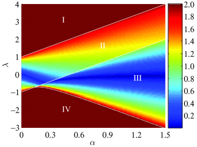
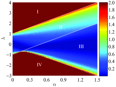
Figure 5: $C_{l_{1}}^{na}(\rho_{i,i+r})$ (top) and $C_{re}^{na}(\rho_{i,i+r})$ (bottom) versus $\alpha$ and $\lambda$ for the three-spin interaction XX model with $N=2001$ and $r=100$. Here, regions I and IV correspond to spin-saturated phase, while regions II and III correspond to two kinds of spin liquid phases.

In Fig. 5, we plot the SQC as functions of $\alpha$ and $\lambda$ for the three-spin interaction XX model with $N=2001$ and $r=100$. As can be seen from this figure, both $C_{l_{1}}^{na}(\rho_{i,i+r})$ and $C_{re}^{na}(\rho_{i,i+r})$ can signal the regions of different phases. To be explicit, when the system is in the spin-saturated phase, the two SQC measures take their values of about 2, while in the two spin liquid phases, one can observe a pronounced decrease of their values. The critical lines (i.e., $\lambda=\lambda_{c_{1}}$ and $\lambda=\lambda_{c_{3}}$) separating the spin-saturated phase from the spin liquid phase correspond to two inflexions of the SQC. For $\alpha>1/8$, the boundary (i.e., $\lambda=\lambda_{c_{2}}$) between the spin liquid I and spin liquid II phases corresponds to another inflexion of the SQC. Besides the three critical lines, there is a critical line indicated by the minimum of the SQC, but as was shown in Ref. epjb , it is not a boundary of QPT.

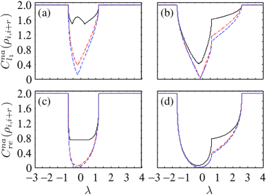
Figure 6: $C_{l_{1}}^{na}(\rho_{i,i+r})$ [panels (a) and (b)] and $C_{re}^{na}(\rho_{i,i+r})$ [panels (c) and (d)] versus $\lambda$ for the three-spin interaction XX model with $N=2001$. Here, $\alpha=0.1$ for panels (a) and (c), $\alpha=0.8$ for panels (b) and (d). The solid black, dash-dotted red, and dashed blue lines (from top to bottom) correspond to $r=1$, 10, and 100, respectively.

To gain more insight into the critical behaviors of SQC for the present model, we further plot in Fig. 6 the dependence of $C_{l_{1}}^{na}(\rho_{i,i+r})$ and $C_{re}^{na}(\rho_{i,i+r})$ on $\lambda$ with different $\alpha$ and $r$. Besides those behaviors observed in Fig. 5, one can observe that when $r=1$ and $\alpha<1/8$, there are two cusplike minima which are pronounced for $C_{l_{1}}^{na}(\rho_{i,i+r})$ and are not obvious for $C_{re}^{na}(\rho_{i,i+r})$, but they are not critical points of QPTs epjb . In this sense, the SQCs of long-distance spin pairs are more reliable than that of the neighboring spin pair in detecting QPTs of the three-spin interaction XX model. Looking at Fig. 6, one can note that the curves of SQC for the spin pairs with different long distances are nearly overlapped; that is, the SQC in this model is also insensitive to the variation of the distance (provided it is not very short) of two spins. Such a property will be useful in the experimental detection of QPTs where other characterizations of quantumness are very weak and hence cannot be detected efficiently.

As for concurrence of $\rho_{i,i+r}$, it is able to detect partial QPTs in the three-spin interaction model for the spin pair with small $r$ XYthree . But when $r$ is large, its value becomes very small, and the regions of non-null concurrence shrink to the vicinity of $\lambda_{c_{2}}$ (if $\alpha<1/8$) or $\lambda_{c_{3}}$ (if $\alpha>1/8$). The quantum discord is a reliable indicator of QPTs when choosing two neighboring spins XYthree , and the two-spin coherence can detect the QPTs as well for small $r$. However, they also decrease with an increase in $r$, especially when $\alpha>1/8$ and $r$ is large, they both oscillate rapidly with respect to $\lambda$ in the region of $\lambda\in(\lambda_{c_{3}},\lambda_{c_{2}})$, with a large number of extreme points being observed. It is therefore hard to distinguish these points from the critical points of QPTs.

Finally, we present an explanation for the underpinning of the observed phenomena in the above subsections, that is, the insensitivity of the SQC to the distance $r$ of two spins in the chain and the divergence in the derivative of the SQC with respect to the magnetic field $\lambda$. For brevity, we consider the Hamiltonian $\hat{H}$ without the three-spin interaction, and the general $\hat{H}$ of Eq. (3) can be analyzed in a similar manner.

First, we explain the insensitivity of the SQC to $r$. As $t_{0z}$ is independent of $r$, one only needs to consider the $r$ dependence of $t_{\mu\mu}$ which are determined by $\{G_{n}\}_{n=-r}^{r}$. From Eq. (11), one can obtain that for $\gamma=0$, $|G_{\pm 1}|$ is maximal among all $\{|G_{n}|\}$ if $\lambda\lesssim 0.6736$ and $|G_{0}|$ is maximal if $\lambda\gtrsim 0.6736$, while for $\gamma\in(0,1]$, $|G_{-1}|$ is maximal if $\lambda<\lambda_{0}$ and $|G_{0}|$ is maximal if $\lambda>\lambda_{0}$, with $\lambda_{0}$ increasing from 0.6736 to 1 when $\gamma$ increases from 0 to 1. Moreover, $|G_{\pm n}|$ with large $n$ are negligible compared with those with small $n$. For example, for the Ising model, we have $G_{n}=-2/[(2n+1)\pi]$ at $\lambda=\lambda_{c}$, $G_{-1}=1$ and $G_{n}=0$ ($n\neq-1$) at $\lambda=0$ in the thermodynamic limit ($N\rightarrow\infty$), while for the XX model, we have $G_{0}=2\theta_{0}/\pi-1$ and $G_{n}=2\sin(n\theta_{0})/(n\pi)$ ($n\neq 0$), where $\theta_{0}=\arccos(\min\{\lambda,1\})$. Therefore, for the Ising model, $|G_{n}/G_{-1}|=1/(2n+1)$ at $\lambda=\lambda_{c}$, and such a ratio will be further decreased when $\lambda$ deviates from $\lambda_{c}$. Similarly, for the XX model, $|G_{n}/G_{\pm 1}|=|\sin(n\theta_{0})|/(n\sin\theta_{0})$ and $|G_{n}/G_{0}|=|\sin(n\theta_{0})|/[n(\pi-2\theta_{0})]$. As a consequence, even when $r$ is very large, only those terms $G_{\pm n}$ with small $n$ dominate in $t_{xx}$ and $t_{yy}$, and this results in the insensitivity of $C_{l_{1}}^{na}(\rho_{i,i+r})$ to large $r$. Moreover, it is easy to see that $t_{zz}$ depends weakly on large $r$, thus $C_{re}^{na}(\rho_{i,i+r})$ is also insensitive to large $r$.

Physically, the insensitivity of the SQC indicator to the distance between the tested spins can also be comprehended from the fact that the SQC is null only for $\rho_{AB}=\rho_{A}\otimes\openone_{2}/2$ as it takes into account the three mutually unbiased bases SQC . That is, it characterizes a more general form of correlation and could exist in a parameter region in which there are no entanglement and quantum discord. In fact, the insensitivity of the SQC indicator to large $r$ also has its roots in the insensitivity of the elements of the reduced density matrices $\rho_{i,i+r}$ with large $r$. But for these $\rho_{i,i+r}$, the entanglement has already disappeared and the quantum discord is very weak. Moreover, some sudden change points of quantum discord may not correspond to QPTs as they are caused by the optimization procedure in its definition Karpat .

Second, we explain the divergence in the derivative of the SQC with respect to $\lambda$. Given that $T=0$, then from Eqs. (9) and (11) one can obtain

$$\frac{\partial{t_{0z}}}{\partial{\lambda}}=\frac{\gamma^{2}}{N}\sum_{k}\frac{\sin^{2}(x_{k})}{\varepsilon_{k}^{3}},$$ (14)

$$\frac{\partial{G_{n}}}{\partial{\lambda}}=\frac{\gamma}{N}\sum_{k}\frac{\epsilon_{k}\sin(nx_{k})\sin(x_{k})-\gamma\cos(nx_{k})\sin^{2}(x_{k})}{\varepsilon_{k}^{3}},$$

from which one can see that both $\partial{t_{0z}}/\partial{\lambda}$ and $\partial{G_{n}}/\partial{\lambda}$ are divergent at $\lambda=\lambda_{c}$ as the two fractions in the above equation approach infinity. For the XX model, one can see more specifically the divergence of $\partial{t_{0z}}/\partial{\lambda}$ and $\partial{G_{n}}/\partial{\lambda}$. This is because in the thermodynamic limit, we have $\partial{t_{0z}}/\partial{\lambda}=-\partial{G_{0}}/\partial{\lambda}=2/(\pi\sqrt{1-\lambda^{2}})$ and $\partial{G_{n}}/\partial{\lambda}=-2\cos(n\theta_{0})/(\pi\sqrt{1-\lambda^{2}})$ ($n\neq 0$). Consequently, there is always a divergence in the derivatives of the SQC due to Eq. (12).

IV Summary and discussion

To summarize, we have proposed to use the SQC as a signature of QPTs in the transverse-field XY model with three-spin interaction. The motivation for considering such a quantumness measure is that it is long ranged and exists in the parameter regions for which there are no quantum correlations. Compared with other signatures of QPTs such as entanglement and quantum discord, our method is powerful due to the following advantages: (i) The SQC and its derivative succeed in detecting precisely all the QPTs in the considered models. (ii) The effectiveness of SQC in detecting QPTs is independent of the distance of two spins, which makes it convenient for practical use as one can choose any two spins other than the restricted short-distance spins. This also differentiates it from concurrence and quantum discord, which decrease rapidly with the increasing distance of two spins and disappear or become infinitesimal when the distance is long. (iii) The SQC is analytically solvable and could be estimated experimentally by local projective measurements and one-qubit tomography. Moreover, the advantage of the SQC method over the simple coherence method may originate from the fact that while quantum coherence reveals only the quantum nature of the whole system under a fixed basis, the SQC takes into account the three mutually unbiased bases and the local operation and classical communication between A and B. As a consequence, it captures a kind of correlation which contains more comprehensive information than that of coherence SQC ; naqc2 ; naqc3 , hence it is capable of distinguishing the subtle nature of a system and is more reliable in reflecting the quantum critical behaviors even when the coherence measures fail to do so.

As the three-spin interaction Hamiltonian may be generated in optical lattices three , we expect our observation can be confirmed in future experiments with state-of-the-art techniques. One step further would be to use the SQC method to investigate QPTs of high-dimensional spin systems and exotic quantum phases in many-body systems such as topological phase transitions topo1 ; topo2 ; topo3 ; topo4 ; topo5 . Moreover, it is also appealing to study the dynamics of the SQC, which may provide an interesting scenario for understanding quantum criticality of many-body systems dyqc1 ; dyqc2 ; dyqc3 .

References

- (1) Z. Ficek and S. Swain, Quantum Interference and Coherence: Theory and Experiments, Springer Series in Optical Sciences (Springer, New York, 2005).
- (2) G. Gour, M. P. Müller, V. Narasimhachar, R. W. Spekkens, and N. Y. Halpern, Phys. Rep. 583, 1 (2015).
- (3) T. Baumgratz, M. Cramer, and M. B. Plenio, Phys. Rev. Lett. 113, 140401 (2014).
- (4) A. Streltsov, G. Adesso, and M. B. Plenio, Rev. Mod. Phys. 89, 041003 (2017).
- (5) M. L. Hu, X. Hu, J. C. Wang, Y. Peng, Y. R. Zhang, and H. Fan, Phys. Rep. 762-764, 1 (2018).
- (6) A. Streltsov, E. Chitambar, S. Rana, M. N. Bera, A. Winter, and M. Lewenstein, Phys. Rev. Lett. 116, 240405 (2016).
- (7) J. Ma, B. Yadin, D. Girolami, V. Vedral, and M. Gu, Phys. Rev. Lett. 116, 160407 (2016).
- (8) M. Hillery, Phys. Rev. A 93, 012111 (2016).
- (9) H. L. Shi, S. Y. Liu, X. H. Wang, W. L. Yang, Z. Y. Yang, and H. Fan, Phys. Rev. A 95, 032307 (2017).
- (10) M. N. Bera, T. Qureshi, M. A. Siddiqui, and A. K. Pati, Phys. Rev. A 92, 012118 (2015).
- (11) E. Bagan, J. A. Bergou, S. S. Cottrell, and M. Hillery, Phys. Rev. Lett. 116, 160406 (2016).
- (12) A. Streltsov, U. Singh, H. S. Dhar, M. N. Bera, and G. Adesso, Phys. Rev. Lett. 115, 020403 (2015).
- (13) X. Qi, T. Gao, and F. Yan, J. Phys. A 50, 285301 (2017).
- (14) D. Mondal, T. Pramanik, and A. K. Pati, Phys. Rev. A 95, 010301(R) (2017).
- (15) M. L. Hu and H. Fan, Phys. Rev. A 98, 022312 (2018).
- (16) M. L. Hu, X. M. Wang, and H. Fan, Phys. Rev. A 98, 032317 (2018).
- (17) K. C. Tan, H. Kwon, C. Y. Park, and H. Jeong, Phys. Rev. A 94, 022329 (2016).
- (18) Y. Yao, X. Xiao, L. Ge, and C. P. Sun, Phys. Rev. A 92, 022112 (2015).
- (19) M. L. Hu and H. Fan, Phys. Rev. A 95, 052106 (2017).
- (20) X. Hu, A. Milne, B. Zhang, and H. Fan, Sci. Rep. 6, 19365 (2015).
- (21) J. Zhang, S. R. Yang, Y. Zhang, and C. S. Yu, Sci. Rep. 7, 45598 (2017)
- (22) X. Hu and H. Fan, Sci. Rep. 6, 34380 (2016).
- (23) J. J. Chen, J. Cui, Y. R. Zhang, and H. Fan, Phys. Rev. A 94, 022112 (2016).
- (24) M. Qin, Z. Ren, and X. Zhang, Phys. Rev. A 98, 012303 (2018).
- (25) A. L. Malvezzi, G. Karpat, B. C. Çakmak, F. F. Fanchini, T. Debarba, and R. O. Vianna, Phys. Rev. B 93, 184428 (2016).
- (26) D. Girolami, Phys. Rev. Lett. 113, 170401 (2014).
- (27) S. Du and Z. Bai, Ann. Phys. (N.Y.) 359, 136 (2015).
- (28) G. Karpat, B. Çakmak, and F. F. Fanchini, Phys. Rev. B 90, 104431 (2014).
- (29) S. G. Lei and P. Q. Tong, Quantum Inf. Process. 15, 1811 (2016).
- (30) Y. C. Li and H. Q. Lin, Sci. Rep. 6, 26365 (2016).
- (31) T. C. Yi, W. L. You, N. Wu, and A. M. Oleś, Phys. Rev. B 100, 024423 (2019).
- (32) W. K. Wootters, Phys. Rev. Lett. 80, 2245 (1998).
- (33) A. Osterloh, L. Amico, G. Falci, and R. Fazio, Nature (Londan) 416, 608 (2002).
- (34) T. J. Osborne and M. A. Nielsen, Phys. Rev. A 66, 032110 (2002).
- (35) S. J. Gu, H. Q. Lin, and Y. Q. Li, Phys. Rev. A 68, 042330 (2003).
- (36) S. J. Gu, G. S. Tian, and H. Q. Lin, Phys. Rev. A 71, 052322 (2005).
- (37) L. Amico, R. Fazio, A. Osterloh, and V. Vedral, Rev. Mod. Phys. 80, 517 (2008).
- (38) H. Ollivier and W. H. Zurek, Phys. Rev. Lett. 88, 017901 (2001).
- (39) L. Henderson and V. Vedral, J. Phys. A 34, 6899 (2001).
- (40) T. Werlang, C. Trippe, G. A. P. Ribeiro, and G. Rigolin, Phys. Rev. Lett. 105, 095702 (2010).
- (41) M. S. Sarandy, Phys. Rev. A 80, 022108 (2009).
- (42) R. Dillenschneider, Phys. Rev. B 78, 224413 (2008).
- (43) J. Maziero, H. C. Guzman, L. C. Céleri, M. S. Sarandy, and R. M. Serra, Phys. Rev. A 82, 012106 (2010).
- (44) Y. C. Li and H. Q. Lin, Phys. Rev. A 83, 052323 (2011).
- (45) B. Q. Liu, B. Shao, J. G. Li, J. Zou, and L. A. Wu, Phys. Rev. A 83, 052112 (2011).
- (46) Y. Huang, New J. Phys. 16, 033027 (2014).
- (47) D. Girolami and G. Adesso, Phys. Rev. A 83, 052108 (2011).
- (48) Y. T. Wang, J. S. Tang, Z. Y. Wei, S. Yu, Z. J. Ke, X. Y. Xu, C. F. Li, and G. C. Guo, Phys. Rev. Lett. 118, 020403 (2017).
- (49) D. J. Zhang, C. L. Liu, X. D. Yu, and D. M. Tong, Phys. Rev. Lett. 120, 170501 (2018).
- (50) X. D. Yu and O. Gühne, Phys. Rev. A 99, 062310 (2019).
- (51) J. K. Pachos and M. B. Plenio, Phys. Rev. Lett. 93, 056402 (2004).
- (52) S. Sachdev, Quantum Phase Transitions (Cambridge University Press, Cambridge, England, 2000).
- (53) I. Titvinidze and G. I. Japaridze, Eur. Phys. J. B 32, 383 (2003).
- (54) X. G. Wang, Phys. Lett. A 331, 164 (2004).
- (55) S. J. Gu, C. P. Sun, and H. Q. Lin, J. Phys. A 41, 025002 (2008).
- (56) E. Barouch, B. M. McCoy, and M. Dresden, Phys. Rev. A 2, 1075 (1970).
- (57) E. Barouch and B. McCoy, Phys. Rev. A 3, 786 (1971).
- (58) P. Pfeuty, Ann. Phys. (N.Y.) 57, 79 (1970).
- (59) M. Zhong and P. Tong, J. Phys. A 43, 505302 (2010).
- (60) B. McCoy, E. Barouch, and D. Abraham, Phys. Rev. A 4, 2331 (1971).
- (61) A. Kitaev and J. Preskill, Phys. Rev. Lett. 96, 110404 (2006).
- (62) A. Hamma, W. Zhang, S. Haas, and D. A. Lidar, Phys. Rev. B 77, 155111 (2008).
- (63) F. Pollmann, A. M. Turner, E. Berg, and M. Oshikawa, Phys. Rev. B 81, 064439 (2010).
- (64) Y. X. Chen and S. W. Li, Phys. Rev. A 81, 032120 (2010).
- (65) J. Cui, J. P. Cao, and H. Fan, Phys. Rev. A 82, 022319 (2010).
- (66) H. T. Quan, Z. Song, X. F. Liu, P. Zanardi, and C. P. Sun, Phys. Rev. Lett. 96, 140604 (2006).
- (67) D. Rossini, T. Calarco, V. Giovannetti, S. Montangero, and R. Fazio, Phys. Rev. A 75, 032333 (2007).
- (68) Z. Sun, X. G. Wang, and C. P. Sun, Phys. Rev. A 75, 062312 (2007).