Exact asymptotics of component-wise extrema of two-dimensional Brownian motion

Abstract: We derive the exact asymptotics of

$$\mathbb{P}\left\{\sup_{t\geq 0}\Bigl{(}X_{1}(t)-\mu_{1}t\Bigr{)}>u,\ \sup_{s\geq 0}\Bigl{(}X_{2}(s)-\mu_{2}s\Bigr{)}>u\right\},\ \ u\to\infty,$$

where $(X_{1}(t),X_{2}(s))_{t,s\geq 0}$ is a correlated two-dimensional Brownian motion with correlation $\rho\in[-1,1]$ and $\mu_{1},\mu_{2}>0$. It appears that the play between $\rho$ and $\mu_{1},\mu_{2}$ leads to several types of asymptotics. Although the exponent in the asymptotics as a function of $\rho$ is continuous, one can observe different types of prefactor functions depending on the range of $\rho$, which constitute a phase-type transition phenomena.

Key Words: Two-dimensional Brownian motion; exact asymptotics; component-wise extrema; quadratic programming problem; generalised Pickands-Piterbarg constants.

AMS Classification: Primary 60G15; secondary 60G70

1. Introduction

Distributional properties of component-wise extrema of stochastic processes attract growing interest in recent literature. On one side, it is a natural object of interest in the extreme value theory of random fields. On the other side, strong motivation to investigate component-wise extrema stems for example from multivariate stochastic models applied to modern multidimensional risk theory, financial mathematics or advanced communication networks, to name some of the applied-probability areas.

We consider a standard correlated Brownian motion $(X_{1}(t),X_{2}(t))_{t\geq 0}$ with constant correlation $\rho\in[-1,1]$, and let $(X_{1}(t),X_{2}(s))_{t,s\geq 0}$ be its two parameter extension, where

$$\mathbb{E}\left\{X_{1}(t)X_{2}(s)\right\}=\rho\min(t,s).$$

The aim of this paper is to find exact asymptotics of

(1) $$P(u):=\mathbb{P}\left\{Q_{1}>u,Q_{2}>u\right\},\qquad u\to\infty,$$

where $Q_{j}=\sup_{t\geq 0}(X_{j}(t)-\mu_{j}t)$ with $\mu_{j}>0$, $j=1,2$.

Due to its importance in, e.g., quantitative finance or ruin theory, the component-wise maxima

$$(Q_{1}(T),Q_{2}(T))=\left(\sup_{t\in[0,T]}(X_{1}(t)-\mu_{1}t),\sup_{s\in[0,T]}(X_{2}(s)-\mu_{2}s)\right)$$

have been studied extensively; see, e.g., [13, 10, 17, 23, 22]. In particular, some formulas for the joint distribution of $(Q_{1}(T),\ Q_{2}(T))$ are known. Unfortunately, they are in the form of infinite-sums of integrals of some special functions, which makes them of limited use in drawing out asymptotic properties of $P(u)$ as $u\to\infty$.

Interestingly, in [13] it was worked out a formula for joint survival function of $(Q_{1}(\mathcal{E}_{p}),Q_{2}(\mathcal{E}_{p}))$, where $\mathcal{E}_{p}$ is an independent exponential random variable with parameter $p>0$. Vector $(Q_{1}(\mathcal{E}_{p}),Q_{2}(\mathcal{E}_{p}))$ as well as $(Q_{1},Q_{2})$ have bivariate exponential distribution (BVE) in the sense of the terminology of Kou and Zhong [13], that is: (i) it has exponential marginals and (ii) it is absolute continuous with respect to two-dimensional Lebesgue measure. The later property for $(Q_{1},Q_{2})$ follows from Theorem 7.1 in [2] combined with the fact that $\mathbb{P}\left\{Q_{j}=0\right\}=0$, see also related Lemma 4.4 in [6]. We remark that requirement (ii) implies that $(Q_{1},Q_{2})$ does not belong to the classical examples of Marshall-Olkin-type BVE; see [16]. Since there are no results in the literature on qualitative properties of our BVE distribution, as a by-product of the results of this contribution, we analyze the dependence structure of $Q_{1}$ and $Q_{2}$ in an asymptotical sense of Resnick [21]; see Remarks 2.2 (b) and Remarks 2.4 (b) for more details. We refer also to a related work of Rogers and Shepp [22] who considered correlation structure of $(Q_{1}(T),Q_{2}(T))$ for two Brownian motions without drift.

A need to consider the joint survival function for $(Q_{1},Q_{2})$ appeared also in Lieshout and Mandjes [14] who considered two parallel queues sharing the same Brownian input (which is the case of $\rho=1$) and also a Brownian tandem queue. We refer to [15] for further discussions on Gaussian-related queueing models and to [3, 5] for the analysis of a related simultaneous ruin problem for the correlated Brownian motion model.

It is worth noting that in recent papers [25, 11], the component-wise maxima in discrete models defined by

$$(\max_{1\leq i\leq n}X_{i}^{1},\ldots,\max_{1\leq i\leq n}X_{i}^{d}),$$

with $(X_{i}^{1},\ldots,X^{d}_{i})$ $(i=1,2,\ldots)$ independent and identically distributed Gaussian random vectors, were discussed.

The first step in understanding the asymptotics of (1) is to find its logarithmic asymptotics. This was done recently in [7], in an insurance context, where $P(u)$ was interpreted as the probability of component-wise ruin. More precisely, by an application of Theorem 1 in [8]

(2) $$\frac{\ln P(u)}{u}\sim-\frac{g(\boldsymbol{t}_{0})}{2},\ \ \ u\to\infty,$$

where

(3) $$g(\boldsymbol{t}_{0})=\inf_{\boldsymbol{t}>\boldsymbol{0}}\inf_{\boldsymbol{v}\geq\boldsymbol{1}+\boldsymbol{\mu}\boldsymbol{t}}\boldsymbol{v}^{\top}\Sigma_{ts}^{-1}\boldsymbol{v}$$

and $\Sigma_{ts}^{-1}$ is the inverse matrix of $\ \Sigma_{ts}=\left(\begin{array}[]{cc}t&\rho\ t\wedge s\\ \rho\ t\wedge s&s\\ \end{array}\right),$ with $\boldsymbol{t}=(t,s)^{\top}$ and $t\wedge s=\min(t,s)$. The main contribution of [7] includes the detailed analysis of the two-layer minimisation problem involved in $g(\boldsymbol{t}_{0})$, which results in an explicit logarithmic asymptotics of $P(u)$; see also Proposition 3.1 below.

In order to get the exact asymptotics of $P(u)$ as $u\to\infty$, we employ a modification of the double-sum technique, accommodated to the analysis of multivariate extremes investigated in this contribution; see Theorems 2.1 and 2.3, which constitute the main results of this paper. It appears that the play between $\rho$ and $\mu_{1},\mu_{2}$ leads to several types of asymptotics. Although in [7] it was noticed, that the exponent in the asymptotics as a function of $\rho$, called therein an adjustment coefficient, is continuous, one can observe different types of prefactor functions depending on the range of $\rho$. This phase-type phenomena has no intuitive explanations.

In the rest of the paper we assume that $\rho\in(-1,1)$ and without loss of generality suppose that $\mu_{1}\leq\mu_{2}$. Note that for $\rho=1$,

$$P(u)=\mathbb{P}\left\{\sup_{s\geq 0}(X_{2}(s)-\mu_{2}s)>u\right\}=e^{-2\mu_{2}u},\ \ \ \forall u>0$$

and, for $\rho=0$,

(4) $$P(u)=\mathbb{P}\left\{\sup_{t\geq 0}(X_{1}(t)-\mu_{1}t)>u\right\}\mathbb{P}\left\{\sup_{s\geq 0}(X_{2}(s)-\mu_{2}s)>u\right\}=e^{-2(\mu_{1}+\mu_{2})u},\ \ \ \forall u>0.$$

To work out the case $\rho=-1$, one can use a result from [24], to show that

(5) $$P(u)\sim e^{-(2\mu_{2}+6\mu_{1})u}(2I_{(\mu_{1}=\mu_{2})}+I_{(\mu_{1}<\mu_{2})}),\ \ \ u\to\infty,$$

where $I_{(\cdot)}$ is the indicator function.

The rest of this paper is organised as follows. In Section 2, we present the exact asymptotics of $P(u)$, given in Theorems 2.1, 2.3. Section 3 recalls the explicit expressions for $g(\boldsymbol{t}_{0})$ and $\boldsymbol{t}_{0}$ derived in [7]. The main lines of proofs are displayed in Section 4 and Section 5, respectively, followed by the Appendix consisting of technical calculations.

We conclude this section by showing some notation and conventions used in this work. All vectors here are $2$-dimensional column vectors written in bold letters. For instance $\boldsymbol{\alpha}=(\alpha_{1},\alpha_{2})^{\top}$, with ^⊤ the transpose sign. Operations with vectors are meant component-wise, so $\lambda\boldsymbol{x}=\boldsymbol{x}\lambda=(\lambda x_{1},\lambda x_{2})^{\top}$ for any $\lambda\in\mathbb{R},\boldsymbol{x}\in\mathbb{R}^{2}$. For any set $D\subseteq[0,\infty)^{2}$, any $\lambda>0$ and any $(a_{1},a_{2})\in[0,\infty)^{2}$ denote

$$\lambda D=\{(\lambda t,\lambda s):(t,s)\in D\},\ \ \ {(a_{1},a_{2})}+D=\{(a_{1}+t,a_{2}+s):(t,s)\in D\}.$$

Next, let us briefly mention the following standard notation for two given positive functions $f(\cdot)$ and $h(\cdot)$. We write $f(x)=h(x)(1+o(1))$ or simply $f(x)\sim h(x)$, if $\lim_{x\to a}{f(x)}/{h(x)}=1$ ($a\in\mathbb{R}\cup\{\infty\}$). Further, write $f(x)=o(h(x))$ if $\lim_{x\to a}{f(x)}/{h(x)}=0$, and write $f(x)\lesssim h(x)$ if $\lim_{x\to a}{f(x)}/{h(x)}\leq 1.$

2. Main results

In this section we present the exact asymptotics of $P(u)$, for which we need some additional notation. First, define

(6) $$\hat{\rho}_{1}=\frac{\mu_{1}+\mu_{2}-\sqrt{(\mu_{1}+\mu_{2})^{2}-4\mu_{1}(\mu_{2}-\mu_{1})}}{4\mu_{1}}\in[0,\frac{1}{2}),\ \ \ \ \ \hat{\rho}_{2}=\frac{\mu_{1}+\mu_{2}}{2\mu_{2}}.$$

These are key points, based on which we consider different scenarios of $\rho$. Next, let

(9) $$\ \Sigma_{*}=\left(\begin{array}[]{cc}t^{*}&\rho s^{*}\\ \rho s^{*}&s^{*}\\ \end{array}\right),\ \ \ \ \ \boldsymbol{b}_{*}=(1+\mu_{1}t^{*},1+\mu_{2}s^{*})^{\top},$$

with

(10) $$t^{*}=t^{*}(\rho)=s^{*}=s^{*}(\rho):=\sqrt{\frac{2(1-\rho)}{\mu_{1}^{2}+\mu_{2}^{2}-2\rho\mu_{1}\mu_{2}}}.$$

Moreover, denote, for any fixed $T,S>0$,

(11) $$\triangle_{T,S}=\{(t,s):t\in[0,T],s\in[t,t+S]\}\cup\{(t,s):s\in[0,T],t\in[s,s+S]\},$$

and define

$$\mathcal{H}(T,S):=\int_{\mathbb{R}^{2}}e^{\boldsymbol{x}^{\top}\Sigma_{*}^{-1}\boldsymbol{b}_{*}}\mathbb{P}\left\{{\underset{(t,s)\in\triangle_{T,S}}{\exists}}\begin{array}[]{ccc}X_{1}(t)-\mu_{1}t>x_{1}\\ X_{2}(s)-\mu_{2}s>x_{2}\end{array}\right\}dx_{1}dx_{2}\in(0,\infty),$$

where the finiteness can be proved by following a standard argument in proving the finiteness of Pickands and Piterbarg type constants; see, e.g., [18] (or Lemma 4.2 in [3]). Interestingly, a new Pickands-Piterbarg constant

$$\widetilde{\mathcal{H}}:=\lim_{S\to\infty}\lim_{T\to\infty}\frac{1}{T}\mathcal{H}(T,S)\in(0,\infty)$$

appears in the scenario $\hat{\rho}_{1}<\rho<\hat{\rho}_{2}$; the existence, finiteness and positiveness of this constant are proved in Theorem 2.1 below.

We split the statement of the main results on the exact asymptotics into two scenarios: $\mu_{1}<\mu_{2}$ and $\mu_{1}=\mu_{2}$ respectively.

Theorem 2.1.

Suppose that $\mu_{1}<\mu_{2}$. We have, as $u\to\infty,$

$$P(u)\sim\left\{\begin{array}[]{ll}e^{-2(\mu_{2}+(1-2\rho)\mu_{1})u},&\hbox{if \ $-1<\rho<\hat{\rho}_{1}$;}\\ \frac{1}{2}\ e^{-2(\mu_{2}+(1-2\hat{\rho}_{1})\mu_{1})u},&\hbox{if \ $\rho=\hat{\rho}_{1}$;}\\ \frac{\widetilde{\mathcal{H}}\sqrt{t^{*}}}{2\sqrt{\pi(1-\rho)}}\ u^{-1/2}e^{-\frac{\mu_{1}+\mu_{2}+2/t^{*}}{1+\rho}u},&\hbox{if \ $\hat{\rho}_{1}<\rho<\hat{\rho}_{2}$;}\\ e^{-2\mu_{2}u},&\hbox{if \ $\hat{\rho}_{2}<\rho<1$,}\end{array}\right.$$

where

$$0<\frac{t^{*}\boldsymbol{\mu}^{\top}\Sigma_{*}^{-1}\boldsymbol{b}_{*}}{16\prod_{i=1}^{2}(\Sigma_{*}^{-1}\boldsymbol{b}_{*})_{i}}<\widetilde{\mathcal{H}}<\infty.$$

Remarks 2.2.

(a). It turns out that the special scenario $\rho=\hat{\rho}_{2}$ is of different nature than the scenarios analyzed in Theorem 2.1. Note that in this case we have $b_{1}=b_{2}=0$ in Lemma A.1, which implies that around its optimizing point $(t^{*},s^{*})=(1/\mu_{2},1/\mu_{2})$ function $g(t,s)$ defined in Section 3 takes different form than for other scenarios. This makes its analysis go out of the approach that works for the other scenarios. In Section 4.4, following the same lines of reasoning as given in the proof of case $\hat{\rho}_{2}<\rho<1$ in Theorem 2.1, we find the following bounds for the case of $\rho=\hat{\rho}_{2}$

(14) $$\frac{1}{2}\ e^{-2\mu_{2}u}\ \lesssim\ P(u)\ \lesssim\ e^{-2\mu_{2}u},\ {\rm as}\ u\to\infty.$$

(b). It follows from Theorem 2.1 and (5) that for any $-1\leq\rho<\hat{\rho}_{2}$

$$\mathbb{P}\left\{Q_{1}(\infty)>u|Q_{2}(\infty)>u\right\}=\frac{\mathbb{P}\left\{Q_{1}(\infty)>u,Q_{2}(\infty)>u\right\}}{\mathbb{P}\left\{Q_{2}(\infty)>u\right\}}\to 0,\ \ u\to\infty.$$

According to the terminology from [21], this means that $Q_{1}(\infty)$ is asymptotically independent of $Q_{2}(\infty)$. Similarly, one can see that $Q_{2}(\infty)$ is also asymptotically independent of $Q_{1}(\infty)$ (note that the notion of asymptotically independence is not symmetric). Furthermore, for $\hat{\rho}_{2}\leq\rho\leq 1$, we have that $Q_{2}(\infty)$ is asymptotically independent of $Q_{1}(\infty)$, but $Q_{1}(\infty)$ is asymptotically dependent of (equivalent to) $Q_{2}(\infty)$.

Next we give the result for the case where $\mu:=\mu_{1}=\mu_{2}$. In this case, we have $t^{*}=s^{*}=1/\mu$ and

$$\widetilde{\mathcal{H}}:=\lim_{S\to\infty}\lim_{T\to\infty}\frac{1}{T}\int_{\mathbb{R}^{2}}e^{\frac{2\mu}{1+\rho}(x_{1}+x_{2})}\mathbb{P}\left\{{\underset{(t,s)\in\triangle_{T,S}}{\exists}}\begin{array}[]{ccc}X_{1}(t)-\mu t>x_{1}\\ X_{2}(s)-\mu s>x_{2}\end{array}\right\}dx_{1}dx_{2}.$$

Theorem 2.3.

Suppose that $\mu_{1}=\mu_{2}$. We have, as $u\to\infty,$

$$P(u)\sim\left\{\begin{array}[]{ll}2\ e^{-4(1-\rho)\mu u},&\hbox{if \ $-1<\rho<0$;}\\ \ e^{-4\mu u},&\hbox{if \ $\rho=0$;}\\ \frac{\widetilde{\mathcal{H}}}{2\sqrt{\pi\mu(1-\rho)}}\ u^{-1/2}e^{-\frac{4\mu}{1+\rho}u},&\hbox{if \ $0<\rho<1$, }\end{array}\right.$$

where $(1+\rho)/{16}<\widetilde{\mathcal{H}}<\infty.$

Remarks 2.4.

(a). Note that comparing scenario $-1<\rho<0$ of Theorem 2.3 with $-1<\rho<\hat{\rho}_{1}$ of Theorem 2.1, there is an additional 2 appearing in the asymptotics. The reason for this is that there are two equally important minimizers of $g(t,s),(t,s)\in(0,\infty)^{2}$ in the case of $\mu_{1}=\mu_{2}$.

(b). For any $-1<\rho<1$, we have that $Q_{1}(\infty)$ and $Q_{2}(\infty)$ are mutually asymptotically independent.

3. Analysis of the two-layer minimization problem

In this section, for completeness and for reference we recall some notation and the result on the two-layer minimization problem (3) derived in [7]. Recall that $g(\boldsymbol{t}_{0})=\inf_{(t,s)\in(0,\infty)^{2}}g(t,s)$ with

$$g(t,s):=\underset{y\geq 1+\mu_{2}s}{\inf_{x\geq 1+\mu_{1}t}}\ (x,y)\ \Sigma_{ts}^{-1}\ (x,y)^{\top},\ \ \ \ \ t,s>0.$$

We define for $t,s>0$ the following functions:

$$g_{1}(t)=\frac{(1+\mu_{1}t)^{2}}{t},\ \ \ \ g_{2}(s)=\frac{(1+\mu_{2}s)^{2}}{s},$$

$$g_{3}(t,s)=(1+\mu_{1}t,1+\mu_{2}s)\ \Sigma_{ts}^{-1}\ (1+\mu_{1}t,1+\mu_{2}s)^{\top}.$$

Since $t\wedge s$ appears in the above formula, we shall consider a partition of the quadrant $(0,\infty)^{2}$, namely

(17) $$(0,\infty)^{2}=A\cup L\cup B,\ \ \ A=\{s<t\},\ L=\{s=t\},\ B=\{s>t\}.$$

For convenience we denote $\overline{A}=\{s\leq t\}=A\cup L$ and $\overline{B}=\{s\geq t\}=B\cup L$. Hereafter, all sets are defined on $(0,\infty)^{2}$, so $(t,s)\in(0,\infty)^{2}$ will be omitted.

Note that $g_{3}(t,s)$ can be represented in the following two different forms:

(20) $$g_{3}(t,s) = \left\{\begin{array}[]{cc}g_{A}(t,s):=\frac{(1+\mu_{1}t)^{2}s-2\rho s(1+\mu_{1}t)(1+\mu_{2}s)+(1+\mu_{2}s)^{2}t}{ts-\rho^{2}s^{2}},&\hbox{if }(t,s)\in\overline{A}\\ g_{B}(t,s):=\frac{(1+\mu_{1}t)^{2}s-2\rho t(1+\mu_{1}t)(1+\mu_{2}s)+(1+\mu_{2}s)^{2}t}{ts-\rho^{2}t^{2}},&\hbox{if }(t,s)\in\overline{B}\end{array}\right.$$

(23) $$= \left\{\begin{array}[]{cc}\frac{(1+\mu_{2}s)^{2}}{s}+\frac{((1+\mu_{1}t)-\rho(1+\mu_{2}s))^{2}}{t-\rho^{2}s},&\hbox{if }(t,s)\in\overline{A}\\ \frac{(1+\mu_{1}t)^{2}}{t}+\frac{((1+\mu_{2}s)-\rho(1+\mu_{1}t))^{2}}{s-\rho^{2}t},&\hbox{if }(t,s)\in\overline{B}.\end{array}\right.$$

Denote further

(24) $$g_{L}(s):=g_{A}(s,s)=g_{B}(s,s)=\frac{(1+\mu_{1}s)^{2}+(1+\mu_{2}s)^{2}-2\rho(1+\mu_{1}s)(1+\mu_{2}s)}{(1-\rho^{2})s},\ \ \ s>0.$$

The following result gives a full analysis of the two-layer minimization problem (3), which is crucial for our derivation of the exact asymptotics of $P(u)$. We refer to [7] for its detailed proof.

Proposition 3.1.

• Suppose that $-1<\rho<0$.
  For $\mu_{1}<\mu_{2}$ we have

  $$g(\boldsymbol{t}_{0})=g_{A}(t_{A},s_{A})=4(\mu_{2}+(1-2\rho)\mu_{1}),$$

  where, $(t_{A},s_{A})=(t_{A}(\rho),s_{A}(\rho)):=\left(\frac{1-2\rho}{\mu_{1}},\frac{1}{\mu_{2}-2\mu_{1}\rho}\right)\in A$ is the unique minimizer of $g(t,s),(t,s)\in(0,\infty)^{2}$.
  For $\mu_{1}=\mu_{2}=:\mu$ we have

  $$g(\boldsymbol{t}_{0})=g_{A}(t_{A},s_{A})=g_{B}(t_{B},s_{B})=8(1-\rho)\mu,$$

  where $(t_{A},s_{A})=\left(\frac{1-2\rho}{\mu},\frac{1}{(1-2\rho)\mu}\right),(t_{B},s_{B}):=\left(\frac{1}{(1-2\rho)\mu},\frac{1-2\rho}{\mu}\right)\in B$ are the only two minimizers of $g(t,s),(t,s)\in(0,\infty)^{2}$.

• Suppose that $0\leq\rho<\hat{\rho}_{1}$. We have

  $$g(\boldsymbol{t}_{0})=g_{A}(t_{A},s_{A})=4(\mu_{2}+(1-2\rho)\mu_{1}),$$

  where $(t_{A},s_{A})$ is the unique minimizer of $g(t,s),(t,s)\in(0,\infty)^{2}$.

• Suppose that $\rho=\hat{\rho}_{1}$. We have

  $$g(\boldsymbol{t}_{0})=g_{A}(t_{A},s_{A})=4(\mu_{2}+(1-2\rho)\mu_{1}),$$

  where $(t_{A},s_{A})=(t_{A}(\hat{\rho}_{1}),s_{A}(\hat{\rho}_{1}))=(t^{*}(\hat{\rho}_{1}),s^{*}(\hat{\rho}_{1}))\in L$, is the unique minimizer of $g(t,s),(t,s)\in(0,\infty)^{2}$, with $(t^{*},s^{*})$ defined in (10).

• Suppose that $\hat{\rho}_{1}<\rho<\hat{\rho}_{2}$. We have

  $$g(\boldsymbol{t}_{0})=g_{A}(t^{*},s^{*})=g_{L}(t^{*})=\frac{2}{1+\rho}(\mu_{1}+\mu_{2}+2/t^{*}),$$

  where $(t^{*},s^{*})\in L$ is the unique minimizer of $g(t,s),(t,s)\in(0,\infty)^{2}$.

• Suppose that $\rho=\hat{\rho}_{2}$. We have $t^{*}(\hat{\rho}_{2})=s^{*}(\hat{\rho}_{2})=1/\mu_{2}$, and

  $$g(\boldsymbol{t}_{0})=g_{A}(1/\mu_{2},1/\mu_{2})=g_{L}(1/\mu_{2})=g_{2}(1/\mu_{2})=4\mu_{2},$$

  where the minimum of $g(t,s),(t,s)\in(0,\infty)^{2}$ is attained at $(1/\mu_{2},1/\mu_{2})$, with $g_{3}(1/\mu_{2},1/\mu_{2})=g_{2}(1/\mu_{2})$, and $1/\mu_{2}$ is the unique minimizer of $g_{2}(s),s\in(0,\infty)$.

• Suppose that $\hat{\rho}_{2}<\rho<1$. We have

  $$g(\boldsymbol{t}_{0})=\inf_{(t,s)\in D_{2}}g_{2}(s)=g_{2}({1}/{\mu_{2}})=4\mu_{2},$$

  where the minimum of $g(t,s),(t,s)\in(0,\infty)^{2}$ is attained when $g(t,s)=g_{2}(s)$.

4. Proof of Theorem 2.1

The proof of Theorem 2.1 will be presented in the order of cases (i) $-1<\rho<\hat{\rho}_{1}$, (ii) $\hat{\rho}_{1}<\rho<\hat{\rho}_{2}$, (iii) $\rho=\hat{\rho}_{1}$, (iv) $\hat{\rho}_{2}\leq\rho<1$ in the following subsections.

Note that by self-similarity

(25) $$P(u)=\mathbb{P}\left\{\exists_{t,s>0}\ (X_{1}(t)>(1+\mu_{1}t)\sqrt{u},\ X_{2}(s)>(1+\mu_{2}s)\sqrt{u})\right\},$$

and recall the notation for the optimizer points $(t_{A},s_{A})$ as introduced in Proposition 3.1.

4.1. (i) Scenario $-1<\rho<\hat{\rho}_{1}$.

4.1.1. Splitting on subregions

We first split the region $(0,\infty)^{2}$ into the following two parts:

$$U_{1}:=[t_{A}-\theta_{0},t_{A}+\theta_{0}]\times[s_{A}-\theta_{0},s_{A}+\theta_{0}]\subset A.\ \ \ U_{2}:=(0,\infty)^{2}\setminus U_{1},$$

where $\theta_{0}>0$ is some small constant which can be identified later on. It follows from (25) that

$$P_{0}(u):=\mathbb{P}\left\{\exists_{(t,s)\in U_{1}}\ X_{1}(t)>\sqrt{u}(1+\mu_{1}t),X_{2}(s)>\sqrt{u}(1+\mu_{2}s)\right\}$$

(26) $$\leq P(u)\leq\mathbb{P}\left\{\exists_{(t,s)\in U_{1}}\ X_{1}(t)>\sqrt{u}(1+\mu_{1}t),X_{2}(s)>\sqrt{u}(1+\mu_{2}s)\right\}$$

$$\ \ \ \ \ \ \ \ \ \ \ \ +\mathbb{P}\left\{\exists_{(t,s)\in U_{2}}\ X_{1}(t)>\sqrt{u}(1+\mu_{1}t),X_{2}(s)>\sqrt{u}(1+\mu_{2}s)\right\}$$

$$=:P_{0}(u)+r_{0}(u)$$

Furthermore, we have, for all large $u$,

(27) $$p(u)\leq P_{0}(u)\leq p(u)+r_{1}(u),$$

where

$$p(u):=\mathbb{P}\left\{\exists_{(t,s)\in\triangle^{(1)}_{u}\times\triangle^{(2)}_{u}}\ X_{1}(t)>\sqrt{u}(1+\mu_{1}t),X_{2}(s)>\sqrt{u}(1+\mu_{2}s)\right\},$$

$$r_{1}(u):=\mathbb{P}\left\{\exists_{(t,s)\in U_{1}\setminus\triangle^{(1)}_{u}\times\triangle_{u}^{(2)}}\ X_{1}(t)>\sqrt{u}(1+\mu_{1}t),X_{2}(s)>\sqrt{u}(1+\mu_{2}s)\right\},$$

with

$$\triangle^{(1)}_{u}=\left[t_{A}-\frac{\ln(u)}{\sqrt{u}},t_{A}+\frac{\ln(u)}{\sqrt{u}}\right],\ \triangle^{(2)}_{u}=\left[s_{A}-\frac{\ln(u)}{\sqrt{u}},s_{A}+\frac{\ln(u)}{\sqrt{u}}\right].$$

Next, we further split the rectangle $\triangle^{(1)}_{u}\times\triangle^{(2)}_{u}$ into smaller rectangles. To this end, we denote, for any fixed $T,S>0$

$$\triangle^{(1)}_{j;u}=\triangle^{(1)}_{j;u}(T)=[t_{A}+jTu^{-1},t_{A}+(j+1)Tu^{-1}],\ \ -N^{(1)}_{u}\leq j\leq N^{(1)}_{u},$$

$$\triangle^{(2)}_{l;u}=\triangle^{(2)}_{l;u}(S)=[s_{A}+lSu^{-1},s_{A}+(l+1)Su^{-1}],\ \ -N^{(2)}_{u}\leq l\leq N^{(2)}_{u},$$

where $N^{(1)}_{u}=\lfloor T^{-1}\ln(u)\sqrt{u}\rfloor$, $N^{(2)}_{u}=\lfloor S^{-1}\ln(u)\sqrt{u}\rfloor$ (we denote by $\lfloor a\rfloor$ the smallest integer that is larger than $a$). Define

$$p_{j,l;u}=\mathbb{P}\left\{\exists_{(t,s)\in\triangle^{(1)}_{j;u}\times\triangle_{l;u}^{(2)}}\ X_{1}(t)>\sqrt{u}(1+\mu_{1}t),X_{2}(s)>\sqrt{u}(1+\mu_{2}s)\right\}$$

and

$$p_{j,l_{1},l_{2};u}=\mathbb{P}\left\{\exists_{t\in\triangle^{(1)}_{j;u}}{X}_{1}(t)>\sqrt{u}(1+\mu_{1}t),\exists_{s\in\triangle^{(2)}_{l_{1};u}}{X}_{2}(s)>\sqrt{u}(1+\mu_{2}s),\exists_{s\in\triangle^{(2)}_{l_{2};u}}{X}_{2}(s)>\sqrt{u}(1+\mu_{2}s)\right\}$$

$$\overline{p}_{j_{1},j_{2},l;u}=\mathbb{P}\left\{\exists_{t\in\triangle^{(1)}_{j_{1};u}}{X}_{1}(t)>\sqrt{u}(1+\mu_{1}t),\exists_{t\in\triangle^{(1)}_{j_{2};u}}{X}_{1}(t)>\sqrt{u}(1+\mu_{1}t),\exists_{s\in\triangle^{(2)}_{l;u}}{X}_{2}(s)>\sqrt{u}(1+\mu_{2}s)\right\}.$$

We have from the generalized Bonferroni’s inequality (see Lemma A.2 in Appendix Proof of Lemma A.1)

(28) $$p_{1}(u)\geq p(u)\geq p_{2}(u)-\Pi_{1}(u)-\Pi_{2}(u),$$

where

$$p_{1}(u)=\sum_{j=-N^{(1)}_{u}}^{N^{(1)}_{u}}\sum_{l=-N^{(2)}_{u}}^{N^{(2)}_{u}}p_{j,l;u},\ \ p_{2}(u)=\sum_{j=-N^{(1)}_{u}+1}^{N^{(1)}_{u}-1}\sum_{l=-N^{(2)}_{u}+1}^{N^{(2)}_{u}-1}p_{j,l;u},$$

$$\Pi_{1}(u)=\sum_{j=-N^{(1)}_{u}}^{N^{(1)}_{u}}\sum_{-N^{(2)}_{u}\leq l_{1}<l_{2}\leq N^{(2)}_{u}}p_{j,l_{1},l_{2};u},\ \ \Pi_{2}(u)=\sum_{l=-N^{(2)}_{u}}^{N^{(2)}_{u}}\sum_{-N^{(1)}_{u}\leq j_{1}<j_{2}\leq N^{(1)}_{u}}\overline{p}_{j_{1},j_{2},l;u}.$$

4.1.2. Upper bounds and estimates

In what follows, we shall derive upper bounds for $r_{0}(u),r_{1}(u)$ in Lemma 4.1, the exact asymptotics of $p_{1}(u),p_{2}(u)$ in Lemma 4.2 and asymptotic behaviour for $\Pi_{1}(u),\Pi_{2}(u)$ in Lemma 4.3. The proofs of the lemmas are displayed in Appendix Proof of Lemma A.1. Recall that we assume $-1<\rho<\hat{\rho}_{1}$.

Lemma 4.1.

For any chosen small $\theta_{0}>0,$ we have, for all large $u$,

$$r_{0}(u)\leq e^{-\frac{(\sqrt{u}-C_{0})^{2}}{2}\widehat{g}},\ \ \text{with}\ \ \widehat{g}=\inf_{(t,s)\in U_{2}}g(t,s)>g_{A}(t_{A},s_{A}),$$

$$r_{1}(u)\leq C_{1}u^{3/2}e^{-\frac{u}{2}g_{A}(t_{A},s_{A})-K_{1}(\ln(u))^{2}}$$

hold for some constants $C_{0},C_{1},K_{1}>0$ not depending on $u$.

Below we discuss the asymptotics of $p_{1}(u),p_{2}(u)$. Define

$$\mathcal{H}(\mu;T):=\int_{\mathbb{R}}e^{2\mu x_{1}}\mathbb{P}\left\{\exists_{t\in[0,T]}\ B_{1}(t)-\mu t>x_{1}\right\}dx_{1}.$$

Lemma 4.2.

We have, as $u\to\infty$,

$$p_{1}(u)\sim p_{2}(u)\sim\frac{\mathcal{H}(\mu_{1};T)\mathcal{H}(\mu_{2}-2\mu_{1}\rho;S)}{TS}\frac{1}{\mu_{1}(\mu_{2}-2\mu_{1}\rho)}e^{-\frac{g_{A}(t_{A},s_{A})}{2}u}.$$

The last lemma is concerned with the asymptotic behaviour of $\Pi_{1}(u),\Pi_{2}(u)$.

Lemma 4.3.

It holds that

$$\limsup_{S\to\infty}\limsup_{T\to\infty}\lim_{u\to\infty}\frac{\Pi_{1}(u)}{\exp(-g_{A}(t_{A},s_{A})u/2)}=\limsup_{S\to\infty}\limsup_{T\to\infty}\lim_{u\to\infty}\frac{\Pi_{2}(u)}{\exp(-g_{A}(t_{A},s_{A})u/2)}=0.$$

4.1.3. Asymptotics of $P(u)$

By Lemmas 4.1, 4.2, 4.3 applied to (4.1.1) - (28) we obtain that

$$P(u)\sim\lim_{S\to\infty}\lim_{T\to\infty}\frac{\mathcal{H}(\mu_{1};T)\mathcal{H}(\mu_{2}-2\mu_{1}\rho;S)}{TS}\frac{1}{\mu_{1}(\mu_{2}-2\mu_{1}\rho)}e^{-\frac{g_{A}(t_{A},s_{A})}{2}u}=e^{-\frac{g_{A}(t_{A},s_{A})}{2}u},$$

where we used that, for any $\mu>0$

(29) $$\mathcal{H}(\mu):=\lim_{T\to\infty}\frac{1}{T}\mathcal{H}(\mu;T)=\mu,$$

see, e.g., [3]. Hence, using that $g_{A}(t_{A},s_{A})=4(\mu_{2}+(1-2\rho)\mu_{1})$ (see (i)-(ii) of Proposition 3.1) we conclude the proof for scenario $-1<\rho<\hat{\rho}_{1}$ in Theorem 2.1. $\Box$

4.2. (ii) Scenario $\hat{\rho}_{1}<\rho<\hat{\rho}_{2}$

4.2.1. Splitting on subregions

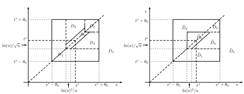
Figure 1. Partition of $(0,\infty)^{2}$: Left for $\hat{\rho}_{1}<\rho<\hat{\rho}_{2}$; right for $\rho=\hat{\rho}_{1}$

We split the region $(0,\infty)^{2}$ into five pieces as shown in Figure 1 (left). Namely, with some small $\theta_{0}>0$ and $u$ large, let

$$D_{0}=\{(t,s):t^{*}-{\ln(u)}/{\sqrt{u}}\leq t\leq t^{*}+{\ln(u)}/{\sqrt{u}},\ 0\leq s-t\leq\ln(u)^{2}/u\}\cup$$

$$\ \ \ \ \ \ \ \ \ \ \ \ \{(t,s):s^{*}-{\ln(u)}/{\sqrt{u}}\leq s\leq s^{*}+{\ln(u)}/{\sqrt{u}},\ 0\leq t-s\leq\ln(u)^{2}/u\},$$

$$D_{2}=\{(t,s):t^{*}+{\ln(u)}/{\sqrt{u}}\leq t\leq t^{*}+\theta_{0},\ s^{*}+{\ln(u)}/{\sqrt{u}}\leq s\leq s^{*}+\theta_{0},\},$$

$$D_{3}=\{(t,s):s^{*}-{\ln(u)}/{\sqrt{u}}\leq s\leq s^{*}+{\ln(u)}/{\sqrt{u}},\ s+{\ln(u)^{2}}/{u}\leq t\leq t^{*}+\theta_{0},\},$$

$$D_{4}=\{(t,s):t^{*}-{\ln(u)}/{\sqrt{u}}\leq t\leq t^{*}+{\ln(u)}/{\sqrt{u}},\ t+{\ln(u)^{2}}/{u}\leq s\leq s^{*}+\theta_{0},\},$$

$$D_{1}=[t^{*}-\theta_{0},t^{*}+\theta_{0}]\times[s^{*}-\theta_{0},s^{*}+\theta_{0}]\setminus(D_{0}\cup D_{2}\cup D_{3}\cup D_{4}),$$

$$D_{5}=(0,\infty)^{2}\setminus[t^{*}-\theta_{0},t^{*}+\theta_{0}]\times[s^{*}-\theta_{0},s^{*}+\theta_{0}].$$

Clearly, we have the following bounds

(30) $$p(u)\leq P(u)\leq p(u)+r_{1}(u)+r_{2}(u)+r_{3}(u),$$

where

$$p(u):=\mathbb{P}\left\{\exists_{(t,s)\in D_{0}}\ X_{1}(t)>\sqrt{u}(1+\mu_{1}t),X_{2}(s)>\sqrt{u}(1+\mu_{2}s)\right\},$$

$$r_{1}(u):=\mathbb{P}\left\{\exists_{(t,s)\in D_{5}}\ X_{1}(t)>\sqrt{u}(1+\mu_{1}t),X_{2}(s)>\sqrt{u}(1+\mu_{2}s)\right\},$$

$$r_{2}(u):=\mathbb{P}\left\{\exists_{(t,s)\in D_{1}\cup D_{2}}\ X_{1}(t)>\sqrt{u}(1+\mu_{1}t),X_{2}(s)>\sqrt{u}(1+\mu_{2}s)\right\},$$

$$r_{3}(u):=\mathbb{P}\left\{\exists_{(t,s)\in D_{3}\cup D_{4}}\ X_{1}(t)>\sqrt{u}(1+\mu_{1}t),X_{2}(s)>\sqrt{u}(1+\mu_{2}s)\right\}.$$

Next, we consider a further partition of $D_{0}$. Recall $\triangle_{T,S}$ given in (11). Denote, for any $T,S>0$ and $u>0,$

$$\triangle^{(1)}_{j;u}=\triangle^{(1)}_{j;u}(T)=[t^{*}+jTu^{-1},t^{*}+(j+1)Tu^{-1}],\ \ -N^{(1)}_{u}\leq j\leq N^{(1)}_{u},$$

$$\triangle^{(2)}_{l;u}=\triangle^{(2)}_{l;u}(S)=[lSu^{-1},(l+1)Su^{-1}],\ \ 1\leq l\leq N_{u}^{(2)},$$

where $N_{u}^{(1)}=\lfloor T^{-1}\ln(u)\sqrt{u}\rfloor$, $N_{u}^{(2)}=\lfloor S^{-1}\ln(u)^{2}\rfloor$. Define further

$$p_{j;u} := \mathbb{P}\left\{\exists_{(t,s)\in(t^{*}+\frac{jT}{u},s^{*}+\frac{jT}{u})+u^{-1}\triangle_{T,S}}\ X_{1}(t)>\sqrt{u}(1+\mu_{1}t),X_{2}(s)>\sqrt{u}(1+\mu_{2}s)\right\},$$

$$p_{j,l;u} := \mathbb{P}\left\{\exists_{t\in\triangle^{(1)}_{j;u},s-t\in\triangle_{l;u}^{(2)}}\ X_{1}(t)>\sqrt{u}(1+\mu_{1}t),X_{2}(s)>\sqrt{u}(1+\mu_{2}s)\right\},$$

$$\overline{p}_{j,l;u} := \mathbb{P}\left\{\exists_{s\in\triangle^{(1)}_{j;u},t-s\in\triangle_{l;u}^{(2)}}\ X_{1}(t)>\sqrt{u}(1+\mu_{1}t),X_{2}(s)>\sqrt{u}(1+\mu_{2}s)\right\},$$

and

$$q_{j_{1},j_{2};u}=\mathbb{P}\left\{\begin{array}[]{cc}\exists_{(t,s)\in(t^{*}+\frac{j_{1}T}{u},s^{*}+\frac{j_{1}T}{u})+u^{-1}\triangle_{T,S}}\ X_{1}(t)>\sqrt{u}(1+\mu_{1}t),X_{2}(s)>\sqrt{u}(1+\mu_{2}s)\\ \exists_{(t,s)\in(t^{*}+\frac{j_{2}T}{u},s^{*}+\frac{j_{2}T}{u})+u^{-1}\triangle_{T,S}}\ X_{1}(t)>\sqrt{u}(1+\mu_{1}t),X_{2}(s)>\sqrt{u}(1+\mu_{2}s)\end{array}\right\}.$$

Thus, it follows from the Bonferroni’s inequality that

(32) $$\overline{\Pi}_{1}(u)+\Pi_{1}(u)+p_{1}(u)\geq p(u)\geq p_{2}(u)-\Pi_{21}(u)-\Pi_{22}(u),$$

where

$$p_{1}(u)=\sum_{j=-N_{u}^{(1)}}^{N_{u}^{(1)}}p_{j;u},\ \ \ \ p_{2}(u)=\sum_{j=-N_{u}^{(1)}+1}^{N_{u}^{(1)}-1}p_{j;u},\ \ \ \ \overline{\Pi}_{1}(u)=\sum_{j=-N_{u}^{(1)}}^{N_{u}^{(1)}}\sum_{1\leq l\leq N_{u}^{(2)}}\overline{p}_{j,l;u},$$

$$\Pi_{1}(u)=\sum_{j=-N_{u}^{(1)}}^{N_{u}^{(1)}}\sum_{1\leq l\leq N_{u}^{(2)}}p_{j,l;u},\ \ \ \ \Pi_{21}(u):=\sum^{N_{u}^{(1)}}_{j_{1}=-N_{u}^{(1)}}\sum_{j_{2}>j_{1}+1}q_{j_{1},j_{2};u},\ \ \ \ \Pi_{22}(u):=\sum^{N_{u}^{(1)}}_{j_{1}=-N_{u}^{(1)}}q_{j_{1},j_{1}+1;u}.$$

4.2.2. Upper bounds and estimates

In what follows, we shall derive upper bounds for $r_{i}(u),i=1,2,3$ in Lemma 4.4, the exact asymptotics of $p_{1}(u),p_{2}(u)$ in Lemma 4.5 and asymptotic behaviour for $\overline{\Pi}_{1}(u),\Pi_{1}(u),\Pi_{21}(u),\Pi_{22}(u)$ in Lemma 4.7. The proofs of the lemmas are displayed in Appendix Proof of Lemma A.1.

Lemma 4.4.

For any chosen small $\theta_{0}>0,$ we have, for all large $u$,

$$r_{1}(u)\leq e^{-\frac{(\sqrt{u}-C_{1})^{2}}{2}\widehat{g}},\ \ \ \widehat{g}=\inf_{(t,s)\in D_{5}}g(t,s)>g_{L}(t^{*}),$$

$$r_{2}(u)\leq C_{2}u^{3/2}e^{-\frac{u}{2}g_{L}(t^{*})-K_{2}(\ln(u))^{2}},$$

$$r_{3}(u)\leq C_{3}u^{3/2}e^{-\frac{u}{2}g_{L}(t^{*})-K_{3}(\ln(u))^{2}}$$

hold for some constants $C_{1},C_{2},C_{3},K_{2},K_{3}>0$ not depending on $u$.

Lemma 4.5.

For any $T,S>0,$ we have, as $u\to\infty$,

$$p_{1}(u)\sim p_{2}(u)\sim\frac{\mathcal{H}(T,S)}{T}\frac{\sqrt{t^{*}}}{2\sqrt{\pi(1-\rho)}}\ u^{-1/2}\ e^{-\frac{ug_{L}(t^{*})}{2}}.$$

Below, we show, for any fixed $S>0$, the sub-additivity property of $\mathcal{H}(T,S)$ as a function of $T>0$.

Lemma 4.6.

Let $S>0$ be fixed, we have for any $T_{1},T_{2}>0$

$$\mathcal{H}(T_{1}+T_{2},S)\leq\mathcal{H}(T_{1},S)+\mathcal{H}(T_{2},S)$$

and further,

$$0<\frac{t^{*}\boldsymbol{\mu}^{\top}\Sigma_{*}^{-1}\boldsymbol{b}_{*}}{16\prod_{i=1}^{2}(\Sigma_{*}^{-1}\boldsymbol{b}_{*})_{i}}<\lim_{T\to\infty}\frac{1}{T}\mathcal{H}(T,S)=\inf_{T>0}\frac{1}{T}\mathcal{H}(T,S)<\infty.$$

The last lemma gives some asymptotic results for $\overline{\Pi}_{1}(u),\Pi_{1}(u),\Pi_{21}(u),\Pi_{22}(u)$.

Lemma 4.7.

For any $T>S>1$,

$$\lim_{u\to\infty}\frac{\max(\Pi_{1}(u),\overline{\Pi}_{1}(u))}{u^{-1/2}\exp(-g_{L}(t^{*})u/2)}\leq C_{0}\lfloor S\rfloor\sum_{l\geq 1}e^{-K_{0}lS},$$

$$\lim_{u\to\infty}\frac{\Pi_{21}(u)}{u^{-1/2}\exp(-g_{L}(t^{*})u/2)}\leq C_{1}(S)\lfloor T\rfloor\sum_{l\geq 1}e^{-K_{1}lT},$$

and

$$\lim_{u\to\infty}\frac{\Pi_{22}(u)}{u^{-1/2}\exp(-g_{L}(t^{*})u/2)}=\frac{\sqrt{t^{*}}}{2\sqrt{\pi(1-\rho)}}\ \left(\frac{2\mathcal{H}(T,S)}{T}-\frac{\mathcal{H}(2T,S)}{T}\right),$$

where $C_{0},K_{0},K_{1}>0$ are three constants which do not dependent on $T,S,u$, and $C_{1}(S)$ does not dependent on $T,u$.

4.2.3. Asymptotics of $P(u)$

Combining (30)-(32) and the results in Lemmas 4.4, 4.5 and 4.7, yields that, for any large $T_{1},T_{2},S_{1},S_{2}$ such that $S_{i}<T_{i},i=1,2$,

$$\frac{\sqrt{t^{*}}}{2\sqrt{\pi(1-\rho)}}\frac{\mathcal{H}(T_{1},S_{1})}{T_{1}}+2C_{0}\lfloor S_{1}\rfloor\sum_{l\geq 1}e^{-K_{0}lS_{1}}$$

$$\geq\limsup_{u\to\infty}\frac{P(u)}{u^{-1/2}\exp(-g_{L}(t^{*})u/2)}\geq\liminf_{u\to\infty}\frac{P(u)}{u^{-1/2}\exp(-g_{L}(t^{*})u/2)}$$

$$\geq\frac{\sqrt{t^{*}}}{2\sqrt{\pi(1-\rho)}}\frac{\mathcal{H}(T_{2},S_{2})}{T_{2}}-C_{1}(S_{2})\lfloor T_{2}\rfloor\ \sum_{k\geq 1}e^{-K_{1}kT_{2}}-\frac{\sqrt{t^{*}}}{2\sqrt{\pi(1-\rho)}}\left(\frac{2\mathcal{H}(T_{2},S_{2})}{T_{2}}-\frac{\mathcal{H}(2T_{2},S_{2})}{T_{2}}\right).$$

Letting first $T_{2}\to\infty$ and then $S_{2}\to\infty$, we have from the above formula, (29) and Lemma 4.6 that

$$\lim_{S\to\infty}\lim_{T\to\infty}\frac{\mathcal{H}(T,S)}{T}\in(0,\infty).$$

The proof for scenario $\hat{\rho}_{1}<\rho<\hat{\rho}_{2}$ in Theorem 2.1 follows then by letting $T_{1}\to\infty$ and then $S_{1}\to\infty$, and (iv) of Proposition 3.1. $\Box$

4.3. (iii) Scenario $\rho=\hat{\rho}_{1}$

Since the idea of the proof of this case is similar to that of scenarios (i) and (ii), we present only main steps. We split the region $(0,\infty)^{2}$ into five pieces as shown in Figure 1 (right). Namely, with some small $\theta_{0}>0$ and $u$ large, let

$$\widetilde{D}_{0}=\{(t,s):t^{*}-{\ln(u)}/{\sqrt{u}}\leq t\leq t^{*}+{\ln(u)}/{\sqrt{u}},\ 0\leq s-t\leq\ln(u)^{2}/u\}\cup$$

$$\ \ \ \ \ \ \ \ \ \ \ \ \{(t,s):s^{*}-{\ln(u)}/{\sqrt{u}}\leq s\leq s^{*}+{\ln(u)}/{\sqrt{u}},\ s<t\leq t^{*}+{\ln(u)}/{\sqrt{u}}\}=:\widetilde{D}_{0B}\cup\widetilde{D}_{0A},$$

$$\widetilde{D}_{3}=\{(t,s):s^{*}-\theta_{0}\leq s\leq s^{*}+\theta_{0},\ s<t\leq t^{*}+\theta_{0}\}\setminus\widetilde{D}_{0A},$$

$$\widetilde{D}_{1}=D_{1}\cap\overline{B},\ \ \ \widetilde{D}_{2}=D_{2}\cap\overline{B},\ \ \ \widetilde{D}_{4}=D_{4},\ \ \ \widetilde{D}_{5}=D_{5}.$$

Clearly, we have the following bounds

(33) $$p(u)\leq P(u)\leq p(u)+\tilde{r}_{0}(u)+\tilde{r}_{1}(u)+\tilde{r}_{2}(u),$$

where

$$p(u):=\mathbb{P}\left\{\exists_{(t,s)\in\widetilde{D}_{0A}}\ X_{1}(t)>\sqrt{u}(1+\mu_{1}t),X_{2}(s)>\sqrt{u}(1+\mu_{2}s)\right\},$$

$$\tilde{r}_{0}(u):=\mathbb{P}\left\{\exists_{(t,s)\in\widetilde{D}_{0B}}\ X_{1}(t)>\sqrt{u}(1+\mu_{1}t),X_{2}(s)>\sqrt{u}(1+\mu_{2}s)\right\},$$

$$\tilde{r}_{1}(u):=\mathbb{P}\left\{\exists_{(t,s)\in\widetilde{D}_{1}\cup\widetilde{D}_{2}\cup\widetilde{D}_{4}\cup\widetilde{D}_{5}}\ X_{1}(t)>\sqrt{u}(1+\mu_{1}t),X_{2}(s)>\sqrt{u}(1+\mu_{2}s)\right\},$$

$$\tilde{r}_{2}(u):=\mathbb{P}\left\{\exists_{(t,s)\in\widetilde{D}_{3}}\ X_{1}(t)>\sqrt{u}(1+\mu_{1}t),X_{2}(s)>\sqrt{u}(1+\mu_{2}s)\right\}.$$

Similar arguments as used in scenarios (i), (ii) give that

(34) $$\lim_{u\to\infty}\frac{p(u)}{\exp\left(-g_{A}(t_{A},s_{A})u/2\right)}=\frac{\mu_{1}^{3/2}(\mu_{2}-2\mu_{1}\rho)^{2}}{2\pi\sqrt{\mu_{2}-2(\mu_{1}+\mu_{2})\rho+3\mu_{1}\rho^{2}}}\int_{\mathbb{R}}\int_{x_{2}}^{\infty}e^{\frac{-(a_{1}x_{1}^{2}-2a_{2}x_{1}x_{2}+a_{3}x_{2}^{2})}{4}}\,dx_{1}dx_{2},$$

and

(35) $$\lim_{u\to\infty}\frac{\tilde{r}_{0}(u)}{u^{-1/2}\exp\left(-g_{A}(t_{A},s_{A})u/2\right)}\leq\frac{\widetilde{\mathcal{H}}\sqrt{t^{*}}}{2\sqrt{\pi(1-\rho)}},$$

and the asymptotically negligibility of $\tilde{r}_{1}(u),\tilde{r}_{2}(u)$. Note that in proving the bound for $\tilde{r}_{2}(u)$, in addition to (45) as in the proof of Lemma 4.1, we also need the fact that (for $t>s$)

$$g_{A}(t_{A}+t,s_{A}+s) \geq g_{A}(t_{A},s_{A})+\frac{a_{1}}{2}(1-\varepsilon)\Bigg{(}\left(t+\frac{\mu_{2}-2\mu_{1}\rho}{\mu_{1}}\rho s\right)^{2}$$

$$\ \ \ \ \ \ \ \ \ \ \ \ \ \ \ \ \ \ \ \ \ \ \ \ \ \ \ \ \ \ \ \ \ +\left(\frac{(\mu_{2}-2\mu_{1}\rho)^{3}(\mu_{2}-2(\mu_{1}+\mu_{2})\rho+3\mu_{1}\rho^{2})}{\mu_{1}^{3}}\right)s^{2}\Bigg{)}.$$

Consequently, the claim follows by formulas (33)-(35) and the asymptotically negligibility of $\tilde{r}_{1}(u),\tilde{r}_{2}(u)$. This completes the proof of scenario $\rho=\hat{\rho}_{1}$ in Theorem 2.1. $\Box$

4.4. (iv) Scenario $\hat{\rho}_{2}\leq\rho<1$

First note that

$$e^{-2\mu_{2}u}=\mathbb{P}\left\{\sup_{s\geq 0}(X_{2}(s)-\mu_{2}s)>u\right\}\geq P(u)\\ \geq\mathbb{P}\left\{\exists_{t\geq 0}\ X_{1}(t)-\mu_{1}t>u,\ X_{2}(t)-\mu_{2}t>u\right\}=:\pi(u).$$

Furthermore, the exact asymptotics for $\pi(u)$ has been discussed in Corollary 4.3 in [12] (where we take $r=0$). Thus, we have, for $\rho=\hat{\rho}_{2}$,

$$\pi(u)\sim\frac{1}{2}e^{-2\mu_{2}u},\ \ \ u\to\infty,$$

and for $\hat{\rho}_{2}<\rho<1$,

$$\pi(u)\sim e^{-2\mu_{2}u},\ \ \ u\to\infty.$$

Therefore, the claims in scenario $\hat{\rho}_{2}<\rho<1$ of Theorem 2.1 and $\hat{\rho}_{2}=\rho$ in (a) of Remark 2.2 follow. $\Box$

5. Proof of Theorem 2.3

For $\mu_{1}=\mu_{2}=\mu$, we have that $\hat{\rho}_{1}=0,\hat{\rho}_{2}=1$. The case $\rho=0$ follows from (4). Thus the interesting scenarios include (i) $-1<\rho<0$ and (ii) $0<\rho<1$. The claim for (ii) $0<\rho<1$ follows directly from (iii) in Theorem 2.1, with $t^{*}=1/\mu$. Next, we shall focus on the proof for (i) $-1<\rho<0$. The proof goes with the same arguments as in the proof of scenario (i) in Theorem 2.1, but now there are two minimizers of the function $g(t,s),(t,s)\in(0,\infty)^{2},$ namely, $(t_{A},s_{A})=(t_{0},s_{0})\in A,(t_{B},s_{B})=(s_{0},t_{0})\in B$, with $t_{0}=\frac{1-2\rho}{\mu},s_{0}=\frac{1}{(1-2\rho)\mu}.$

We first split the region $(0,\infty)^{2}$ into three parts. Namely, with some small $\theta_{0}>0$, let

$$U_{11}=[t_{0}-\theta_{0},t_{0}+\theta_{0}]\times[s_{0}-\theta_{0},s_{0}+\theta_{0}]\subset A,$$

$$U_{12}=[s_{0}-\theta_{0},s_{0}+\theta_{0}]\times[t_{0}-\theta_{0},t_{0}+\theta_{0}]\subset B,$$

$$U_{2}=(0,\infty)^{2}\setminus(U_{11}\cup U_{12}).$$

As in the proof of scenario (i) of Theorem 2.1, the main contribution of the asymptotics comes from $U_{11}\cup U_{12}$. Note further that

$$\mathbb{P}\left\{\exists_{(t,s)\in(U_{11}\cup U_{12})}\ X_{1}(t)>\sqrt{u}(1+\mu_{1}t),X_{2}(s)>\sqrt{u}(1+\mu_{2}s)\right\}$$

$$= \mathbb{P}\left\{\exists_{(t,s)\in U_{11}}\ X_{1}(t)>\sqrt{u}(1+\mu_{1}t),X_{2}(s)>\sqrt{u}(1+\mu_{2}s)\right\}$$

$$+\mathbb{P}\left\{\exists_{(t,s)\in U_{12}}\ X_{1}(t)>\sqrt{u}(1+\mu_{1}t),X_{2}(s)>\sqrt{u}(1+\mu_{2}s)\right\}$$

$$-\mathbb{P}\left\{\begin{array}[]{cc}\exists_{(t_{1},s_{1})\in U_{11}}\ X_{1}(t_{1})>\sqrt{u}(1+\mu_{1}t_{1}),X_{2}(s_{1})>\sqrt{u}(1+\mu_{2}s_{1})\\ \exists_{(t_{2},s_{2})\in U_{12}}\ X_{1}(t_{2})>\sqrt{u}(1+\mu_{1}t_{2}),X_{2}(s_{2})>\sqrt{u}(1+\mu_{2}s_{2})\end{array}\right\}$$

$$=: P_{\theta_{0},1}(u)+P_{\theta_{0},2}(u)-P_{\theta_{0},0}(u).$$

By symmetric property of the model we know that $P_{\theta_{0},1}(u)=P_{\theta_{0},2}(u)$. Next, we show in Lemma 5.1 that $P_{\theta_{0},0}(u)$ is asymptotically negligible compared with $P_{\theta_{0},1}(u)$. The proof of it is displayed in Appendix Proof of Lemma A.1.

Lemma 5.1.

For any chosen small $\theta_{0}>0,$ we have for all large $u$

$$P_{\theta_{0},0}(u)\leq e^{-\frac{(\sqrt{u}-C_{0})^{2}g_{A}(t_{A},s_{A})}{2\sigma_{0}^{2}}}$$

holds for some constant $C_{0}>0,\sigma_{0}^{2}\in(0,1)$ which do not depend on $u$.

The rest of the proof is the same as those in the proof of scenario (i) in Theorem 2.1, and thus omitted. This completes the proof. $\Box$

Appendix A Proofs of Lemmas 4.1-5.1

In this section we give proofs of Lemmas 4.1-5.1 that are the building blocks of the proofs of Theorems 2.1 and 2.3.

We begin with the analysis of the local behaviour of function $g(t,s),(t,s)\in(0,\infty)$ at its minimizer in scenarios (i)–(iv) of Proposition 3.1, respectivelly.

Lemma A.1.

Assume that $\mu_{1}<\mu_{2}$. We have

• If $-1<\rho<\hat{\rho}_{1}$, then as $(t,s)\to(0,0)$,

  $$g(t_{A}+t,s_{A}+s)=g_{A}(t_{A},s_{A})+\frac{a_{1}}{2}t^{2}(1+o(1))-a_{2}ts(1+o(1))+\frac{a_{3}}{2}s^{2}(1+o(1)),$$

  where, with $h(\rho):=\mu_{2}-2(\mu_{1}+\mu_{2})\rho+3\mu_{1}\rho^{2}>0,$

  $$a_{1}:=\frac{2\mu_{1}^{3}(\mu_{2}-2\mu_{1}\rho)}{h(\rho)}>0,\ \ a_{2}:=\frac{-2\rho\mu_{1}^{2}(\mu_{2}-2\mu_{1}\rho)^{2}}{h(\rho)},\ \ a_{3}:=\frac{2(\mu_{2}-2\mu_{1}\rho)^{4}(1-2\rho)}{h(\rho)}>0.$$

• If $\hat{\rho}_{1}<\rho<\hat{\rho}_{2}$, then

  • (ii.1), as $(t,s)\to(0,0)$, with $s<t$ (i.e., $(t^{*}+t,s^{*}+s)\in A$),

    $$g(t^{*}+t,s^{*}+s)=g_{L}(t^{*})+b_{1}(t-s)(1+o(1))+\frac{c_{1}}{2}s^{2}(1+o(1)),$$

    where

    $$b_{1} := \frac{(\rho-1-2\rho^{2})+2\rho(\mu_{2}-\mu_{1}\rho)s^{*}+(1+\rho)\mu_{1}^{2}{s^{*}}^{2}}{(1-\rho)(1+\rho)^{2}{s^{*}}^{2}}>0,$$

    $$c_{1} := \frac{2}{{s^{*}}^{3}}\left(1+\frac{\rho^{2}(\rho(1-\rho)-(\mu_{2}-\mu_{1}\rho)s^{*})^{2}}{(1-\rho^{2})^{3}}\right)>0.$$

  • (ii.2), as $(t,s)\to(0,0)$, with $s>t$ (i.e., $(t^{*}+t,s^{*}+s)\in B$),

    $$g(t^{*}+t,s^{*}+s)=g_{L}(t^{*})+b_{2}(s-t)(1+o(1))+\frac{c_{2}}{2}t^{2}(1+o(1)),$$

    where

    $$b_{2} := \frac{(\rho-1-2\rho^{2})+2\rho(\mu_{1}-\mu_{2}\rho)t^{*}+(1+\rho)\mu_{2}^{2}{t^{*}}^{2}}{(1-\rho)(1+\rho)^{2}{t^{*}}^{2}}>0,$$

    $$c_{2} := \frac{2}{{t^{*}}^{3}}\left(1+\frac{\rho^{2}(\rho(1-\rho)-(\mu_{1}-\mu_{2}\rho)t^{*})^{2}}{(1-\rho^{2})^{3}}\right)>0.$$

  • (ii.3), as $(t,s)\to(0,0)$, with $s=t$ (i.e., $(t^{*}+t,s^{*}+s)\in L$),

    $$g(t^{*}+t,s^{*}+t)=g_{L}(t^{*})+\frac{b_{0}}{2}t^{2}(1+o(1)),$$

    where $b_{0}:=\frac{4}{(1+\rho){t^{*}}^{3}}.$

• If $\rho=\hat{\rho}_{1}$ (in this case $t_{A}=s_{A}=t^{*}=s^{*}$), then

  • (iii.1), as $(t,s)\to(0,0)$, with $s<t$,

    $$g(t_{A}+t,s_{A}+s)=g_{A}(t_{A},s_{A})+\frac{a_{1}}{2}t^{2}(1+o(1))-a_{2}ts(1+o(1))+\frac{a_{3}}{2}s^{2}(1+o(1)),$$

  • (iii.2), as $(t,s)\to(0,0)$, with $s>t$,

    $$g(t^{*}+t,s^{*}+s)=g_{L}(t^{*})+b_{2}(s-t)(1+o(1))+\frac{c_{2}}{2}t^{2}(1+o(1)).$$

  • (iii.3), as $(t,s)\to(0,0)$, with $s=t$,

    $$g(t^{*}+t,s^{*}+t)=g_{L}(t^{*})+\frac{b_{0}}{2}t^{2}(1+o(1)).$$

The proof of Lemma A.1 is tedious but only involves basic calculations using Taylor expansion, and thus it is omitted.

Next we present below a generalized version of the Bonferroni’s inequality. The proof can be found in, e.g., [9].

Lemma A.2.

Let $(\Omega,\mathcal{F},\mathbb{P})$ be a probability space and $A_{1},\cdots,A_{n}$ and $B_{1},\cdots,B_{m}$ be $n+m$ events in $\mathcal{F}$ with $n,m\geq 2$. Then

$$\sum_{k=1}^{n}\sum_{l=1}^{m}\mathbb{P}\left\{A_{k}\cap B_{l}\right\}\geq\mathbb{P}\left\{\underset{l=1,\ldots,m}{\underset{k=1,\ldots,n}{\bigcup}}(A_{k}\cap B_{l})\right\}\geq\sum_{k=1}^{n}\sum_{l=1}^{m}\mathbb{P}\left\{A_{k}\cap B_{l}\right\}$$

$$\ \ \ \qquad-\sum_{k=1}^{n}\sum_{1\leq l_{1}<l_{2}\leq m}\mathbb{P}\left\{A_{k}\cap B_{l_{1}}\cap B_{l_{2}}\right\}-\sum_{l=1}^{m}\sum_{1\leq k_{1}<k_{2}\leq n}\mathbb{P}\left\{A_{k_{1}}\cap A_{k_{2}}\cap B_{l}\right\}.$$

A.1. Proof of Lemma 4.1

Let $T_{0}>0$ be a fixed large constant (will be determined later). It is easily seen that

$$r_{0}(u) \leq \mathbb{P}\left\{\exists_{(t,s)\in[0,T_{0}]^{2}\setminus U_{1}}\ X_{1}(t)>\sqrt{u}(1+\mu_{1}t),X_{2}(s)>\sqrt{u}(1+\mu_{2}s)\right\}$$

$$+\mathbb{P}\left\{\exists_{t\geq T_{0}}\ X_{1}(t)>\sqrt{u}(1+\mu_{1}t)\right\}+\mathbb{P}\left\{\exists_{s\geq T_{0}}\ X_{2}(s)>\sqrt{u}(1+\mu_{2}s)\right\}.$$

Next we consider upper bounds for each term on the right-hand side. According to Lemma 5 of [7], for any fixed $t,s$, there exists a unique index set

$$I(t,s)\subseteq\{1,2\}$$

such that

(37) $$g(t,s)=(1+\mu_{1}t,1+\mu_{2}s)_{I(t,s)}\ (\Sigma_{ts})_{{I(t,s)},{I(t,s)}}^{-1}\ (1+\mu_{1}t,1+\mu_{2}s)_{I(t,s)}^{\top},$$

and

(38) $$(\Sigma_{ts})_{{I(t,s)},{I(t,s)}}^{-1}\ (1+\mu_{1}t,1+\mu_{2}s)_{I(t,s)}^{\top}>\boldsymbol{0}_{I(t,s)}.$$

Thus,

$$\mathbb{P}\left\{\exists_{(t,s)\in[0,T_{0}]^{2}\setminus U_{1}}\ X_{1}(t)>\sqrt{u}(1+\mu_{1}t),X_{2}(s)>\sqrt{u}(1+\mu_{2}s)\right\}$$

(39) $$\leq\mathbb{P}\left\{\exists_{(t,s)\in[0,T_{0}]^{2}\setminus U_{1}}\ (1+\mu_{1}t,1+\mu_{2}s)_{I(t,s)}\ (\Sigma_{ts})_{{I(t,s)},{I(t,s)}}^{-1}\ (X_{1}(t),X_{2}(s))_{I(t,s)}^{\top}>\sqrt{u}g(t,s)\right\}$$

$$=\mathbb{P}\left\{\exists_{(t,s)\in[0,T_{0}]^{2}\setminus U_{1}}\ \frac{Z(t,s)}{g(t,s)}>\sqrt{u}\right\},$$

where

(40) $$Z(t,s):=(1+\mu_{1}t,1+\mu_{2}s)_{I(t,s)}\ (\Sigma_{ts})_{{I(t,s)},{I(t,s)}}^{-1}\ (X_{1}(t),X_{2}(s))_{I(t,s)}^{\top}.$$

Note that

(41) $$\mathrm{Var}\left(\frac{Z(t,s)}{g(t,s)}\right)=\frac{1}{g(t,s)}.$$

In order to apply the Borell-TIS inequality, we first show that

$$\limsup_{(t,s)\to(t^{(b)},s^{(b)})}\frac{\left\lvert Z(t,s)\right\rvert}{g(t,s)}<\infty,\ \ \ \ \text{almost\ surely}$$

holds for any $(t^{(b)},s^{(b)})$ on the boundary $\{(t,s):t\geq 0,s=0\}\cup\{(t,s):t=0,s\geq 0\}$.
In fact, if the above does not hold for some boundary point $(t^{(b)},s^{(b)})$, then for any $M>0$ there exist a sequence $\{(t_{k},s_{k})\}_{k=1}^{\infty}$ and some measurable set $E$ such that $(t_{k},s_{k})\to(t^{(b)},s^{(b)})$, $\mathbb{P}\left\{E\right\}>0$ and

$$\frac{\left\lvert Z(t_{k},s_{k})\right\rvert}{g(t_{k},s_{k})}\geq M\ \ \ \text{on}\ E$$

for all large enough $k$. Then we have

(42) $$\mathrm{Var}\left(\frac{Z(t_{k},s_{k})}{g(t_{k},s_{k})}\right)\geq M^{2}\mathbb{P}\left\{E\right\}>0.$$

On the other hand, by Lemma 6 of [7] we have $g(t,s)=g_{3}(t,s)$ for all $(t,s)\in\{(t,s):t\geq 0,s=0\}\cup\{(t,s):t=0,s\geq 0\}$, and thus by (41) and (23) we have $\lim_{k\to\infty}\mathrm{Var}\left(\frac{Z(t_{k},s_{k})}{g(t_{k},s_{k})}\right)=0$. This is a contradiction with (42). Therefore, $\frac{Z(t,s)}{g(t,s)},(t,s)\in[0,T_{0}]^{2}\setminus U_{1}$ is almost surely bounded. Consequently, by the Borell-TIS inequality (see, e.g., [1]) we have, for any fixed small constant $\theta_{0}>0$

$$\mathbb{P}\left\{\exists_{(t,s)\in[0,T_{0}]^{2}\setminus U_{1}}\ \frac{Z(t,s)}{g(t,s)}>\sqrt{u}\right\}\leq e^{-\frac{(\sqrt{u}-C_{0})^{2}}{2}\widehat{g}}$$

holds for all $u$ such that

$$\sqrt{u}>C_{0}:=\mathbb{E}\left\{\sup_{(t,s)\in[0,T_{0}]^{2}\setminus U_{1}}\frac{Z(t,s)}{g(t,s)}\right\}.$$

Moreover, since $X_{i}$ is the standard Brownian motion,

$$\lim_{t\to\infty}\frac{X_{i}(t)}{1+\mu_{i}t}=0\ \ \ \ \mathrm{almost\ surely},$$

showing that the random process $\frac{X_{i}(t)}{1+\mu_{i}t},t\geq T_{0}$ has almost surely bounded sample paths on $[T_{0},\infty)$. Again by the Borell-TIS inequality

$$\mathbb{P}\left\{\exists_{t\geq T_{0}}\ X_{i}(t)>\sqrt{u}(1+\mu_{i}t)\right\}\leq e^{-\frac{(\sqrt{u}-C_{i})^{2}}{2}\frac{(1+\mu_{i}T_{0})^{2}}{T_{0}}}$$

holds for all $\sqrt{u}>C_{i}:=\mathbb{E}\left\{\sup_{t\in[T_{0},\infty)}\frac{X_{1}(t)}{1+\mu_{i}t}\right\}$. Since for all large enough $T_{0}$ it holds that $\frac{(1+\mu_{i}T_{0})^{2}}{T_{0}}>\widehat{g},$ the claim for $r_{0}(u)$ is established.

Below we consider $r_{1}(u)$. Since $(t_{A},s_{A})\in A$, we have from Proposition 3.1 that for any chosen small $\theta_{0}$

$$g(t,s)=g_{A}(t,s),\ \ (t,s)\in U_{1}\subset A,$$

and further (cf. (40))

$$Z(t,s)=(1+\mu_{1}t,1+\mu_{2}s)\ \Sigma_{ts}^{-1}\ (X_{1}(t),X_{2}(s))^{\top}=:h_{1}(t,s)X_{1}(t)+h_{2}(t,s)X_{2}(s),\ \ (t,s)\in U_{1},$$

with

$$h_{1}(t,s)=\frac{(1+\mu_{1}t)s-\rho s(1+\mu_{2}s))}{ts-\rho^{2}s^{2}},\ \ \ h_{2}(t,s)=\frac{(1+\mu_{2}s)t-\rho s(1+\mu_{1}t))}{ts-\rho^{2}s^{2}}.$$

Thus, similarly to (A.1) we conclude that

(43) $$r_{1}(u)\leq\mathbb{P}\left\{\exists_{(t,s)\in U_{1}\setminus\triangle^{(1)}_{u}\times\triangle_{u}^{(2)}}\ \frac{Z(t,s)}{g_{A}(t,s)}>\sqrt{u}\right\}.$$

Since $h_{1}(t,s),h_{2}(t,s),g_{A}(t,s),(t,s)\in U_{1}$ are all smooth functions and

$$\mathbb{E}\left\{(X_{i}(t_{1})-X_{i}(t_{2}))^{2}\right\}=\left\lvert t_{1}-t_{2}\right\rvert,\ \ i=1,2$$

one can check that, for all $(t_{1},s_{1}),(t_{2},s_{2})\in U_{1},$

$$\mathbb{E}\left\{\left(\frac{Z(t_{1},s_{1})}{g_{A}(t_{1},s_{1})}-\frac{Z(t_{2},s_{2})}{g_{A}(t_{2},s_{2})}\right)^{2}\right\}\leq\mathrm{Const}\cdot(\left\lvert t_{1}-t_{2}\right\rvert+\left\lvert s_{1}-s_{2}\right\rvert).$$

Therefore, an application of the Piterbarg’s inequality in [4][Lemma 5.1] (see also [18][Theorem 8.1] or [20][Theorem 3]) yields that

(44) $$r_{1}(u)\leq\mathbb{P}\left\{\exists_{(t,s)\in U_{1}\setminus\triangle^{(1)}_{u}\times\triangle_{u}^{(2)}}\ \frac{Z(t,s)}{g_{A}(t,s)}>\sqrt{u}\right\}\leq C_{3}u^{3/2}e^{-\frac{u}{2}\widetilde{g}_{u}},$$

where $C_{3}>0$ is some constant which does not depend on $u$ and

$$\widetilde{g}_{u}:=\inf_{(t,s)\in U_{1}\setminus\triangle^{(1)}_{u}\times\triangle_{u}^{(2)}}g_{A}(t,s).$$

Moreover, we have from (i) of Lemma A.1 that for all $(t_{A}+t,s_{A}+s)\in U_{1}$

(45) $$g_{A}(t_{A}+t,s_{A}+s) \geq g_{A}(t_{A},s_{A})+\frac{a_{1}}{2}(1-\varepsilon)\Bigg{(}(1-\rho^{2})t^{2}+\left(\rho t+\frac{\mu_{2}-2\mu_{1}\rho}{\mu_{1}}s\right)^{2}$$

$$\ \ \ \ \ \ \ \ \ \ \ \ \ \ \ \ \ \ \ \ \ \ \ \ \ \ \ \ \ \ \ \ \ +\left(\frac{\mu_{2}-2\mu_{1}\rho}{\mu_{1}}\right)^{2}\left(\frac{\mu_{2}-2\mu_{1}\rho}{\mu_{1}}(1-2\rho)-1\right)s^{2}\Bigg{)}$$

holds with some small $\varepsilon>0$, where for all $-1<\rho<\hat{\rho}_{1}$ (see also the proof of (b).(i) in Lemma 9 of [7] for $\rho>0$)

$$\frac{\mu_{2}-2\mu_{1}\rho}{\mu_{1}}(1-2\rho)-1>0.$$

Thus

$$\widetilde{g}_{u}\geq g_{A}(t_{A},s_{A})+\frac{a_{1}}{2}(1-\varepsilon)\min\left((1-\rho^{2}),\left(\frac{\mu_{2}-2\mu_{1}\rho}{\mu_{1}}\right)^{2}\left(\frac{\mu_{2}-2\mu_{1}\rho}{\mu_{1}}(1-2\rho)-1\right)\right)\frac{(\ln(u))^{2}}{u}.$$

Inserting the above to (44) completes the proof. $\Box$

A.2. Proof of Lemma 4.2

We first analyze the summand $p_{j,l;u}$. We set

(46) $$\boldsymbol{b}_{j,l;u}=(a_{j;u},b_{l;u})^{\top},\ \ \ \ a_{j;u}=1+\mu_{1}(t_{A}+\frac{jT}{u}),\ \ b_{l;u}=1+\mu_{2}(s_{A}+\frac{lS}{u}).$$

It follows that

(49) $$p_{j,l;u} = \mathbb{P}\left\{\underset{s\in[0,S]}{\exists_{t\in[0,T]}}\begin{array}[]{ccc}X_{1}(t_{A}+\frac{jT}{u}+\frac{t}{u})>a_{j;u}\sqrt{u}+\frac{\mu_{1}}{\sqrt{u}}t\\ X_{2}(s_{A}+\frac{lS}{u}+\frac{s}{u})>b_{l;u}\sqrt{u}+\frac{\mu_{2}}{\sqrt{u}}s\end{array}\right\}$$

(52) $$= \mathbb{P}\left\{\underset{s\in[0,S]}{\exists_{t\in[0,T]}}\begin{array}[]{ccc}X_{1}(t_{A}+\frac{jT}{u})+X_{1}(t_{A}+\frac{jT}{u}+\frac{t}{u})-X_{1}(t_{A}+\frac{jT}{u})>a_{j;u}\sqrt{u}+\frac{\mu_{1}}{\sqrt{u}}t\\ X_{2}(s_{A}+\frac{lS}{u})+X_{2}(s_{A}+\frac{lS}{u}+\frac{s}{u})-X_{2}(s_{A}+\frac{lS}{u})>b_{l;u}\sqrt{u}+\frac{\mu_{2}}{\sqrt{u}}s\end{array}\right\}.$$

Since $(t_{A}+\frac{jT}{u},s_{A}+\frac{lS}{u})\in A$ for all large $u,$ the covariance matrix of $\boldsymbol{Z}_{j,l;u}:=(X_{1}(t_{A}+\frac{jT}{u}),X_{2}(s_{A}+\frac{lS}{u}))^{\top}$ is given by

$$\ \Sigma_{j,l;u}=\left(\begin{array}[]{cc}t_{A}+\frac{jT}{u}&\rho\ (s_{A}+\frac{lS}{u})\\ \rho\ (s_{A}+\frac{lS}{u})&s_{A}+\frac{lS}{u}\\ \end{array}\right).$$

Thus, the density function of $\boldsymbol{Z}_{j,l;u}$ is given by

$$\phi_{\Sigma_{j,l;u}}(\boldsymbol{w})=\frac{1}{\sqrt{(2\pi)^{2}\left\lvert\Sigma_{j,l;u}\right\rvert}}\exp\left(-\frac{1}{2}\boldsymbol{w}^{\top}(\Sigma_{j,l;u})^{-1}\boldsymbol{w}\right),\ \ \ \boldsymbol{w}=(w_{1},w_{2})^{\top}.$$

By conditioning on the value of $\boldsymbol{Z}_{j,l;u}$ we rewrite (49) as

$$p_{j,l;u}=\int_{\mathbb{R}^{2}}\phi_{\Sigma_{j,l;u}}(\boldsymbol{w})\mathbb{P}\left\{\underset{s\in[0,S]}{\exists_{t\in[0,T]}}\begin{array}[]{ccc}X_{1}(t_{A}+\frac{jT}{u}+\frac{t}{u})-X_{1}(t_{A}+\frac{jT}{u})>a_{j;u}\sqrt{u}+\frac{\mu_{1}}{\sqrt{u}}t-w_{1}\\ X_{2}(s_{A}+\frac{lS}{u}+\frac{s}{u})-X_{2}(s_{A}+\frac{lS}{u})>b_{l;u}\sqrt{u}+\frac{\mu_{2}}{\sqrt{u}}s-w_{2}\end{array}\Bigg{|}\boldsymbol{Z}_{j,l;u}=\boldsymbol{w}\right\}\,d\boldsymbol{w},$$

Using change of variables $\boldsymbol{w}=\sqrt{u}\boldsymbol{b}_{j,l;u}-\boldsymbol{x}/\sqrt{u}$ we further obtain

$$p_{j,l;u}=u^{-1}\int_{\mathbb{R}^{2}}\phi_{\Sigma_{j,l;u}}(\sqrt{u}\boldsymbol{b}_{j,l;u}-\boldsymbol{x}/\sqrt{u})P_{j,l;u}(\boldsymbol{x})\,d\boldsymbol{x},$$

where

$$P_{j,l;u}(\boldsymbol{x}):=\mathbb{P}\left\{\underset{s\in[0,S]}{\exists_{t\in[0,T]}}\begin{array}[]{ccc}X_{1}(t_{A}+\frac{jT}{u}+\frac{t}{u})-X_{1}(t_{A}+\frac{jT}{u})>\frac{\mu_{1}}{\sqrt{u}}t+\frac{x_{1}}{\sqrt{u}}\\ X_{2}(s_{A}+\frac{lS}{u}+\frac{s}{u})-X_{2}(s_{A}+\frac{lS}{u})>\frac{\mu_{2}}{\sqrt{u}}s+\frac{x_{2}}{\sqrt{u}}\end{array}\Bigg{|}\boldsymbol{Z}_{j,l;u}=\sqrt{u}\boldsymbol{b}_{j,l;u}-\frac{\boldsymbol{x}}{\sqrt{u}}\right\}.$$

Now, we analyse $P_{j,l;u}(\boldsymbol{x})$. Due to the fact that $(t_{A},s_{A})\in A$, we have for all $t\in[0,T],s\in[0,S]$, and large enough $u$

$$t_{A}+\frac{jT}{u}+\frac{t}{u}\geq t_{A}+\frac{jT}{u}>s_{A}+\frac{lS}{u}+\frac{s}{u}\geq s_{A}+\frac{lS}{u}.$$

Thus, by the properties of Brownian motion

$$P_{j,l;u}(\boldsymbol{x}) = \mathbb{P}\left\{\exists_{t\in[0,T]}\ X_{1}(t)-\mu_{1}t>x_{1}\right\}$$

$$\times\mathbb{P}\left\{\exists_{s\in[0,S]}\ X_{2}(s_{A}+\frac{lS}{u}+\frac{s}{u})-X_{2}(s_{A}+\frac{lS}{u})>\frac{\mu_{2}}{\sqrt{u}}s+\frac{x_{2}}{\sqrt{u}}\Big{|}\boldsymbol{Z}_{j,l;u}=\sqrt{u}\boldsymbol{b}_{j,l;u}-\frac{\boldsymbol{x}}{\sqrt{u}}\right\},$$

Next we have

$$\phi_{\Sigma_{j,l;u}}(\sqrt{u}\boldsymbol{b}_{j,l;u}-\boldsymbol{x}/\sqrt{u})=\frac{1}{\sqrt{(2\pi)^{2}\left\lvert\Sigma_{j,l;u}\right\rvert}}\exp\left(-\frac{1}{2}(\sqrt{u}\boldsymbol{b}_{j,l;u}-\boldsymbol{x}/\sqrt{u})^{\top}(\Sigma_{j,l;u})^{-1}(\sqrt{u}\boldsymbol{b}_{j,l;u}-\boldsymbol{x}/\sqrt{u})\right),$$

where the exponent can be rewritten as

$$(\sqrt{u}\boldsymbol{b}_{j,l;u}-\boldsymbol{x}/\sqrt{u})^{\top}(\Sigma_{j,l;u})^{-1}(\sqrt{u}\boldsymbol{b}_{j,l;u}-\boldsymbol{x}/\sqrt{u})$$

$$=u(\boldsymbol{b}_{j,l;u})^{\top}\Sigma_{j,l;u}^{-1}\boldsymbol{b}_{j,l;u}-2\boldsymbol{x}^{\top}\Sigma_{j,l;u}^{-1}\boldsymbol{b}_{j,l;u}+\frac{1}{u}\boldsymbol{x}^{\top}\Sigma_{j,l;u}^{-1}\boldsymbol{x}$$

$$=ug_{A}(t_{A}+\frac{jT}{u},s_{A}+\frac{lS}{u})-2\boldsymbol{x}^{\top}\Sigma_{j,l;u}^{-1}\boldsymbol{b}_{j,l;u}+\frac{1}{u}\boldsymbol{x}^{\top}\Sigma_{j,l;u}^{-1}\boldsymbol{x}.$$

Define

$$f_{j,l;u}(\boldsymbol{x}):=\exp\left(\boldsymbol{x}^{\top}\Sigma_{j,l;u}^{-1}\boldsymbol{b}_{j,l;u}-\frac{1}{2u}\boldsymbol{x}^{\top}\Sigma_{j,l;u}^{-1}\boldsymbol{x}\right),\ \ \ \ \boldsymbol{x}\in\mathbb{R}^{2}.$$

Thus, it follows that

$$p_{1}(u)=\frac{u^{-1}}{2\pi}\sum_{j=-N^{(1)}_{u}}^{N^{(1)}_{u}}\sum_{l=-N^{(2)}_{u}}^{N^{(2)}_{u}}\frac{1}{\sqrt{\left\lvert\Sigma_{j,l;u}\right\rvert}}\exp\left(-\frac{1}{2}ug_{A}(t_{A}+\frac{jT}{u},s_{A}+\frac{lS}{u})\right)\int_{\mathbb{R}^{2}}f_{j,l;u}(\boldsymbol{x})P_{j,l;u}(\boldsymbol{x})\,d\boldsymbol{x}.$$

Further, we obtain from (i) of Lemma A.1 that, for all large enough $u$,

$$g_{A}(t_{A}+\frac{jT}{u},s_{A}+\frac{lS}{u})\sim g_{A}(t_{A},s_{A})+\frac{1}{2}\left(a_{1}\left(\frac{jT}{u}\right)^{2}-2a_{2}\left(\frac{jT}{u}\right)\left(\frac{lS}{u}\right)+a_{3}\left(\frac{lS}{u}\right)^{2}\right)$$

holds uniformly for $-N_{u}^{(1)}\leq j\leq N_{u}^{(1)},-N_{u}^{(2)}\leq l\leq N_{u}^{(2)}.$

Consequently, by Lemma A.3 below we obtain

$$\lim_{u\to\infty}\frac{p_{1}(u)}{\exp\left(-g_{A}(t_{A},s_{A})u/{2}\right)}=\frac{1}{2\pi\sqrt{\left\lvert\Sigma_{0}\right\rvert}}\frac{\mathcal{H}(\mu_{1};T)\mathcal{H}(\mu_{2}-2\mu_{1}\rho;S)}{TS}\int_{\mathbb{R}^{2}}e^{\frac{-(a_{1}x_{1}^{2}-2a_{2}x_{1}x_{2}+a_{3}x_{2}^{2})}{4}}\,d\boldsymbol{x},$$

which gives the result for $p_{1}(u)$. The claim for $p_{2}(u)$ follows with the same arguments. $\Box$

Lemma A.3.

For any $T,S>0$

$$\lim_{u\to\infty}\int_{\mathbb{R}^{2}}f_{j,l;u}(\boldsymbol{x})P_{j,l;u}(\boldsymbol{x})\,d\boldsymbol{x}=\mathcal{H}(\mu_{1};T)\mathcal{H}(\mu_{2}-2\mu_{1}\rho;S)$$

holds uniformly for $-N_{u}^{(1)}\leq j\leq N_{u}^{(1)},-N_{u}^{(2)}\leq l\leq N_{u}^{(2)}.$

We omit the tedious proof of Lemma A.3 since its idea is standard, i.e., it is based on finding a uniform integrable bound for the integrand and then using the dominated convergence theorem.

A.3. Proof of Lemma 4.3

Let us begin with $\Pi_{1}(u)$. It follows that

$$\Pi_{1}(u) = \sum_{j=-N^{(1)}_{u}}^{N^{(1)}_{u}}\sum_{-N^{(2)}_{u}\leq l_{1}<l_{2}\leq N^{(2)}_{u}}p_{j,l_{1},l_{2};u}$$

$$= \sum_{j=-N^{(1)}_{u}}^{N^{(1)}_{u}}\sum_{l=-N^{(2)}_{u}}^{N^{(2)}_{u}}p_{j,l,l+1;u}+\sum_{j=-N^{(1)}_{u}}^{N^{(1)}_{u}}\sum_{l_{1}=-N^{(2)}_{u}}^{N^{(2)}_{u}}\sum_{l_{2}=l_{1}+2}^{N^{(2)}_{u}}p_{j,l_{1},l_{2};u}=:\Pi_{11}(u)+\Pi_{12}(u).$$

In order to deal with $\Pi_{11}(u)$ we note that

$$p_{j,l,l+1;u}=p_{j,l;u}+p_{j,l+1;u}-\widetilde{p}_{j,l;u},$$

where

$$\widetilde{p}_{j,l;u}=\mathbb{P}\left\{\exists_{(t,s)\in\triangle^{(1)}_{j;u}\times(\triangle_{l;u}^{(2)}\cup\triangle_{l+1;u}^{(2)})}\ X_{1}(t)>\sqrt{u}(1+\mu_{1}t),X_{2}(s)>\sqrt{u}(1+\mu_{2}s)\right\}.$$

Then we have

$$\Pi_{11}(u)=\sum_{j=-N^{(1)}_{u}}^{N^{(1)}_{u}}\sum_{l=-N^{(2)}_{u}}^{N^{(2)}_{u}}(p_{j,l;u}+p_{j,l+1;u}-\widetilde{p}_{j,l;u}).$$

Using the same arguments as in the proof of Lemma 4.2 we obtain

$$\lim_{u\to\infty}\frac{\Pi_{11}(u)}{e^{-g_{A}(t_{A},s_{A})u/2}}=\frac{1}{\mu_{1}(\mu_{2}-2\mu_{1}\rho)}\left(\frac{2\mathcal{H}(\mu_{1};T)\mathcal{H}(\mu_{2}-2\mu_{1}\rho;S)}{TS}-\frac{\mathcal{H}(\mu_{1};T)\mathcal{H}(\mu_{2}-2\mu_{1}\rho;2S)}{TS}\right),$$

which gives that

$$\limsup_{S\to\infty}\limsup_{T\to\infty}\lim_{u\to\infty}\frac{\Pi_{11}(u)}{e^{-g_{A}(t_{A},s_{A})u/2}}=0.$$

Next we consider $\Pi_{12}(u)$ which is more involved. We have (recall (46) for $a_{j;u},b_{l;u}$)

(58) $$p_{j,l_{1},l_{2};u} = \mathbb{P}\left\{\underset{s_{2}\in[0,S]}{\underset{s_{1}\in[0,S]}{\underset{t\in[0,T]}{\exists}}}\begin{array}[]{ccc}X_{1}(t_{A}+\frac{jT}{u}+\frac{t}{u})>a_{j;u}\sqrt{u}+\frac{\mu_{1}}{\sqrt{u}}t\\ X_{2}(s_{A}+\frac{l_{1}S}{u}+\frac{s_{1}}{u})>{\color[rgb]{0,0,0}b_{l_{1};u}}\sqrt{u}+\frac{\mu_{2}}{\sqrt{u}}s_{1}\\ X_{2}(s_{A}+\frac{l_{2}S}{u}+\frac{s_{2}}{u})>b_{l_{2};u}\sqrt{u}+\frac{\mu_{2}}{\sqrt{u}}s_{2}\end{array}\right\}$$

(61) $$\leq \mathbb{P}\left\{\underset{s_{2}\in[0,S]}{\underset{s_{1}\in[0,S]}{\underset{t\in[0,T]}{\exists}}}\begin{array}[]{cc}X_{1}(t_{A}+\frac{jT}{u}+\frac{t}{u})>a_{j;u}\sqrt{u}+\frac{\mu_{1}}{\sqrt{u}}t\\ \frac{1}{2}\left(X_{2}(s_{A}+\frac{l_{1}S}{u}+\frac{s_{1}}{u})+X_{2}(s_{A}+\frac{l_{2}S}{u}+\frac{s_{2}}{u})\right)>b_{l_{1},l_{2};u}\sqrt{u}+\frac{\mu_{2}}{2\sqrt{u}}(s_{1}+s_{2})\end{array}\right\}=:P_{j,l_{1},l_{2};u},$$

with

$$b_{l_{1},l_{2};u}=1+\mu_{2}\left(s_{A}+\frac{l_{1}S}{u}+\frac{(l_{2}-l_{1})S}{2u}\right).$$

For notational simplicity, we shall denote

$$\widetilde{t_{A}}=t_{A}+\frac{jT}{u},\ \ \widetilde{s_{A}}=s_{A}+\frac{l_{1}S}{u},\ \ \overline{s_{A}}=\widetilde{s_{A}}+\frac{(l_{2}-l_{1})S}{2u},\ \ \widehat{s_{A}}=\widetilde{s_{A}}+\frac{(l_{2}-l_{1})S}{4u}.$$

Again by conditioning on the event

$$E_{j,l_{1},l_{2};u}(x_{1},x_{2}):=\left\{X_{1}(\widetilde{t_{A}})=a_{j;u}\sqrt{u}-\frac{x_{1}}{\sqrt{u}},\ \ \ \frac{1}{2}\left(X_{2}(\widetilde{s_{A}})+X_{2}(s_{A}+\frac{l_{2}S}{u})\right)=b_{l_{1},l_{2};u}\sqrt{u}-\frac{x_{2}}{\sqrt{u}}\right\},$$

we have

$$P_{j,l_{1},l_{2};u}=u^{-1}\int_{\mathbb{R}^{2}}\phi_{\Sigma_{j,l_{1},l_{2};u}}(\sqrt{u}\boldsymbol{b}_{j,l_{1},l_{2};u}-\boldsymbol{x}/\sqrt{u})F(j,l_{1},l_{2};u,\boldsymbol{x})\,d\boldsymbol{x},$$

where

$$\Sigma_{j,l_{1},l_{2};u}=\left(\begin{array}[]{cc}\widetilde{t_{A}}&\rho\ \overline{s_{A}}\\ \rho\ \overline{s_{A}}&\widehat{s_{A}}\\ \end{array}\right),\ \ \ \boldsymbol{b}_{j,l_{1},l_{2};u}=(a_{j;u},b_{l_{1},l_{2};u})^{\top}$$

and

$$F(j,l_{1},l_{2};u,\boldsymbol{x}):=\mathbb{P}\left\{\exists_{t\in[0,T]}\ X_{1}(t)-\mu_{1}t>x_{1}\right\}\ \mathbb{P}\left\{\underset{s_{2}\in[0,S]}{\underset{s_{1}\in[0,S]}{\exists}}Y_{j,l_{1},l_{2};u}(s_{1},s_{2})>x_{2}\ \Bigg{|}E_{j,l_{1},l_{2};u}(x_{1},x_{2})\right\},$$

where

$$Y_{j,l_{1},l_{2};u}(s_{1},s_{2})=\frac{\sqrt{u}}{2}\left(X_{2}(\widetilde{s_{A}}+\frac{s_{1}}{u})-X_{2}(\widetilde{s_{A}})+X_{2}(s_{A}+\frac{l_{2}S}{u}+\frac{s_{2}}{u})-X_{2}(s_{A}+\frac{l_{2}S}{u})\right)-\frac{\mu_{2}}{2}(s_{1}+s_{2}).$$

Similarly as in the proof of Lemma 4.2, we obtain

$$\phi_{\Sigma_{j,l_{1},l_{2};u}}(\sqrt{u}\boldsymbol{b}_{j,l_{1},l_{2};u}-\boldsymbol{x}/\sqrt{u})=\frac{1}{\sqrt{(2\pi)^{2}\left\lvert\Sigma_{j,l_{1},l_{2};u}\right\rvert}}\exp\left(-\frac{1}{2}u\ (\boldsymbol{b}_{j,l_{1},l_{2};u})^{\top}\Sigma_{j,l_{1},l_{2};u}^{-1}\boldsymbol{b}_{j,l_{1},l_{2};u}\right)\ f_{j,l_{1},l_{2};u}(\boldsymbol{x}),$$

where

$$f_{j,l_{1},l_{2};u}(\boldsymbol{x}):=\exp\left(\boldsymbol{x}^{\top}\Sigma_{j,l_{1},l_{2};u}^{-1}\boldsymbol{b}_{j,l_{1},l_{2};u}-\frac{1}{2u}\boldsymbol{x}^{\top}\Sigma_{j,l_{1},l_{2};u}^{-1}\boldsymbol{x}\right).$$

Next, some elementary calculations give that

$$(\boldsymbol{b}_{j,l_{1},l_{2};u})^{\top}\Sigma_{j,l_{1},l_{2};u}^{-1}\boldsymbol{b}_{j,l_{1},l_{2};u}=g_{A}(t_{A}+\frac{jT}{u},s_{A}+\frac{l_{1}S}{u}+\frac{(l_{2}-l_{1})S}{2u})+\frac{\widetilde{t_{A}}g_{A}(\widetilde{t_{A}},\overline{s_{A}})-a_{j;u}^{2}}{4(\widetilde{t_{A}}\widehat{s_{A}}-\rho^{2}{\overline{s_{A}}}^{2})}\ \frac{(l_{2}-l_{1})S}{u}.$$

Further, note that

$$g_{A}(t_{A}+\frac{jT}{u},s_{A}+\frac{l_{1}S}{u}+\frac{(l_{2}-l_{1})S}{2u})=g_{A}(t_{A}+\frac{jT}{u},s_{A}+\frac{l_{1}S}{u})+\frac{\partial g_{A}(t,s)}{\partial s}\mid_{(\widetilde{t_{A}},\widetilde{s_{A}}+\theta_{l_{1},l_{2};u}\frac{(l_{2}-l_{1})S}{2u})}\frac{(l_{2}-l_{1})S}{2u}$$

holds for some $\theta_{l_{1},l_{2};u}\in(0,1)$ and

$$\frac{\partial g_{A}(t,s)}{\partial t}\mid_{(\widetilde{t_{A}},\widetilde{s_{A}}+\theta_{l_{1},l_{2};u}\frac{(l_{2}-l_{1})S}{2u})}\ \ \to\ 0,\ \ \ \ u\to\infty$$

holds uniformly for $j,l_{1},l_{2}$ (hereafter when we write $j,l_{1},l_{2}$ we mean $-N^{(1)}_{u}\leq j\leq N^{(1)}_{u},-N^{(2)}_{u}\leq l_{1},l_{2}\leq N^{(2)}_{u}$)).

Consequently

(63) $$\exp\left(-\frac{1}{2}u\ (\boldsymbol{b}_{j,l_{1},l_{2};u})^{\top}\Sigma_{j,l_{1},l_{2};u}^{-1}\boldsymbol{b}_{j,l_{1},l_{2};u}\right)\sim\exp\left(-\frac{1}{2}u\ g_{A}(t_{A}+\frac{jT}{u},s_{A}+\frac{l_{1}S}{u})\right)e^{-Q_{0}(l_{2}-l_{1})S}$$

holds uniformly for $j,l_{1},l_{2}$ as $u\to\infty$, where (by (b).(i) of Lemma 9 of [7] or Lemma A.1.(i) with $a_{1}>0$)

$$Q_{0}=\frac{t_{A}g_{A}(t_{A},s_{A})-(1+\mu_{1}t_{A})^{2}}{8(t_{A}s_{A}-\rho^{2}s_{A}^{2})}>0.$$

Next, we consider the uniform, in $j,l_{1},l_{2}$, limit of the following:

$$\mathbb{P}\left\{\underset{s_{2}\in[0,S]}{\underset{s_{1}\in[0,S]}{\exists}}Y_{j,l_{1},l_{2};u}(s_{1},s_{2})>x_{2}\ \Bigg{|}E_{j,l_{1},l_{2};u}(x_{1},x_{2})\right\},\ \ \ u\to\infty$$

For the conditional mean we can derive that

$$\mathbb{E}\left\{Y_{j,l_{1},l_{2};u}(s_{1},s_{2}){\mid}E_{j,l_{1},l_{2};u}(x_{1},x_{2})\right\} = -\frac{\mu_{2}}{2}(s_{1}+s_{2})$$

$$+\left(\frac{\rho(s_{1}+s_{2})}{2\sqrt{u}},\frac{s_{1}}{4\sqrt{u}}\right)\ \Sigma_{j,l_{1},l_{2};u}^{-1}(\boldsymbol{b}_{j,l_{1},l_{2};u}-\boldsymbol{x}/\sqrt{u}),$$

which further gives that

$$\mathbb{E}\left\{Y_{j,l_{1},l_{2};u}(s_{1},s_{2}){\mid}E_{j,l_{1},l_{2};u}(x_{1},x_{2})\right\}=-\frac{\mu_{2}}{2}(s_{1}+s_{2})+\frac{2\rho a_{j;u}\widehat{s_{A}}-\rho a_{j;u}\overline{s_{A}}-2\rho^{2}b_{j,l_{1},l_{2};u}\overline{s_{A}}+b_{j,l_{1},l_{2};u}\widetilde{t_{A}}}{4(\widetilde{t_{A}}\widehat{s_{A}}-\rho^{2}{\overline{s_{A}}}^{2})}s_{1}$$

$$\ \ \ \ \ \ \ \ \ \ \ +\frac{\rho a_{j;u}\widehat{s_{A}}-\rho^{2}b_{j,l_{1},l_{2};u}\overline{s_{A}}}{2(\widetilde{t_{A}}\widehat{s_{A}}-\rho^{2}{\overline{s_{A}}}^{2})}s_{2}+\frac{\rho\overline{s_{A}}s_{1}-2\rho\widehat{s_{A}}(s_{1}+s_{2})}{4(\widetilde{t_{A}}\widehat{s_{A}}-\rho^{2}{\overline{s_{A}}}^{2})}\ \frac{x_{1}}{u}+\frac{2\rho^{2}\overline{s_{A}}(s_{1}+s_{2})-\widetilde{t_{A}}s_{1}}{4(\widetilde{t_{A}}\widehat{s_{A}}-\rho^{2}{\overline{s_{A}}}^{2})}\ \frac{x_{2}}{u}$$

$$\ \ \ \ \ \ \ \ \ \ \ \to-\frac{1}{2}\left(\mu_{2}-2\mu_{1}\rho\right)s_{2},\ \ \ \ u\to\infty.$$

For the conditional variance of the increments we have

$$\mathrm{Var}\left\{Y_{j,l_{1},l_{2};u}(s_{1},s_{2})-Y_{j,l_{1},l_{2};u}(s^{\prime}_{1},s^{\prime}_{2}){\mid}E_{j,l_{1},l_{2};u}(x_{1},x_{2})\right\}=\frac{\left\lvert s_{1}-s^{\prime}_{1}\right\rvert+\left\lvert s_{2}-s^{\prime}_{2}\right\rvert}{4}$$

$$\ \ \ \ \ \ \ \ \ \ \ \ \ \ \ \ \ \ \ \ +\left(\frac{\rho(s_{1}-s^{\prime}_{1}+s_{2}-s^{\prime}_{2})}{2\sqrt{u}},\frac{s_{1}-s^{\prime}_{1}}{4\sqrt{u}}\right)\Sigma_{j,l_{1},l_{2};u}^{-1}\left(\frac{\rho(s_{1}-s^{\prime}_{1}+s_{2}-s^{\prime}_{2})}{2\sqrt{u}},\frac{s_{1}-s^{\prime}_{1}}{4\sqrt{u}}\right)^{\top}$$

$$\ \ \ \ \ \ \ \ \ \ \ \ \ \ \ \ \ \ \ \ \to\frac{\left\lvert s_{1}-s^{\prime}_{1}\right\rvert+\left\lvert s_{2}-s^{\prime}_{2}\right\rvert}{4},\ \ \ u\to\infty.$$

Therefore, similarly as in Lemma A.3 we can show that as $u\to\infty$

$$\mathbb{P}\left\{\underset{s_{2}\in[0,S]}{\underset{s_{1}\in[0,S]}{\exists}}Y_{j,l_{1},l_{2};u}(s_{1},s_{2})>x_{2}\ \Bigg{|}E_{j,l_{1},l_{2};u}(x_{1},x_{2})\right\}\ \to\ \mathbb{P}\left\{\underset{s_{2}\in[0,S]}{\underset{s_{1}\in[0,S]}{\exists}}\frac{1}{2}(B_{1}(s_{1})+B_{2}(s_{2}))-\frac{1}{2}\left(\mu_{2}-2\mu_{1}\rho\right)s_{2}>x_{2}\right\}.$$

Consequently, the dominated convergence theorem gives

$$\int_{\mathbb{R}^{2}}f_{j,l_{1},l_{2};u}(\boldsymbol{x})F(j,l_{1},l_{2};u,\boldsymbol{x})\,d\boldsymbol{x}$$

$$\to\int_{\mathbb{R}}e^{2\mu_{1}x_{1}}\mathbb{P}\left\{\exists_{t\in[0,T]}\ X_{1}(t)-\mu_{1}t>x_{1}\right\}dx_{1}$$

(64) $$\ \ \ \ \ \times\int_{\mathbb{R}}e^{2(\mu_{2}-2\mu_{1}\rho)x_{2}}\mathbb{P}\left\{\underset{s_{2}\in[0,S]}{\underset{s_{1}\in[0,S]}{\exists}}\frac{1}{2}(B_{1}(s_{1})+B_{2}(s_{2}))-\frac{1}{2}\left(\mu_{2}-2\mu_{1}\rho\right)s_{2}>x_{2}\right\}dx_{2}$$

$$=:\mathcal{H}(\mu_{1};T)\ \mathcal{H}(\mu_{1},\mu_{2};S)$$

holds uniformly for $j,l_{1},l_{2}$, as $u\to\infty$.

Next we derive a useful upper bound for $\mathcal{H}(\mu_{1},\mu_{2};S)$, $S>0$:

(65) $$\mathcal{H}(\mu_{1},\mu_{2};S)\leq(\lfloor S\rfloor)^{2}e^{Q_{0}S}\mathcal{H}(\mu_{1},\mu_{2};1)<\infty.$$

In order to prove (65), by taking $j=l_{1}=0,l_{2}=1$ we arrive at

(68) $$P_{0,0,1;u} = \mathbb{P}\left\{\underset{s_{2}\in[0,S]}{\underset{s_{1}\in[0,S]}{\underset{t\in[0,T]}{\exists}}}\begin{array}[]{cc}X_{1}(t_{A}+\frac{t}{u})>a_{0;u}\sqrt{u}+\frac{\mu_{1}}{\sqrt{u}}t\\ \frac{1}{2}(X_{2}(s_{A}+\frac{s_{1}}{u})+X_{2}(s_{A}+\frac{S}{u}+\frac{s_{2}}{u}))>b_{0,1;u}\sqrt{u}+\frac{\mu_{2}}{2\sqrt{u}}(s_{1}+s_{2})\end{array}\right\}$$

(69) $$\sim \frac{u^{-1}}{\sqrt{(2\pi)^{2}\left\lvert\Sigma_{0,0,0;u}\right\rvert}}\exp\left(-\frac{1}{2}u\ g_{A}(t_{A},s_{A})\right)e^{-Q_{0}S}\mathcal{H}(\mu_{1};T)\mathcal{H}(\mu_{1},\mu_{2};S).$$

Define, for any integers $0\leq m,n\leq\lfloor S\rfloor$,

$$q_{m,n;u}:=\mathbb{P}\left\{\underset{s_{2}\in[0,1]}{\underset{s_{1}\in[0,1]}{\underset{t\in[0,T]}{\exists}}}\begin{array}[]{cc}X_{1}(t_{A}+\frac{t}{u})>a_{0;u}\sqrt{u}+\frac{\mu_{1}}{\sqrt{u}}t\\ \frac{1}{2}(X_{2}(s_{A}+\frac{m}{u}+\frac{s_{1}}{u})+X_{2}(s_{A}+\frac{S+n}{u}+\frac{s_{2}}{u}))>\widetilde{b}_{m,n;u}\sqrt{u}+\frac{\mu_{2}}{2\sqrt{u}}(s_{1}+s_{2})\end{array}\right\}$$

with

$$\widetilde{b}_{m,n;u}=1+\mu_{2}\left(s_{0}+\frac{m}{u}+\frac{S+n-m}{2u}\right).$$

Using the same arguments as in the derivation of (68) one can show that

(71) $$q_{m,n;u}\sim\frac{u^{-1}}{\sqrt{(2\pi)^{2}\left\lvert\Sigma_{0,0,0;u}\right\rvert}}\exp\left(-\frac{1}{2}u\ g_{A}(t_{A},s_{A})\right)e^{-Q_{0}(S+n-m)}\mathcal{H}(\mu_{1};T)\mathcal{H}(\mu_{1},\mu_{2};1).$$

Comparing (68) and (71) we derive

$$\mathcal{H}(\mu_{1},\mu_{2};S) \leq \sum_{m=0}^{\lfloor S\rfloor-1}\sum_{n=0}^{\lfloor S\rfloor-1}e^{-Q_{0}(n-m)}\mathcal{H}(\mu_{1},\mu_{2};1)$$

$$\leq (\lfloor S\rfloor)^{2}e^{Q_{0}S}\mathcal{H}(\mu_{1},\mu_{2};1).$$

The finiteness of $\mathcal{H}(\mu_{1},\mu_{2};1)$ can be proved by using the Borell-TIS inequality. This justifies bound (65).

Now, we are ready to analyse the triple sum $\Pi_{12}(u)$. We have

$$\Pi_{12}(u) = \sum_{j=-N^{(1)}_{u}}^{N^{(1)}_{u}}\sum_{l_{1}=-N^{(2)}_{u}}^{N^{(2)}_{u}}\sum_{l_{2}=l_{1}+2}^{N^{(2)}_{u}}\frac{u^{-1}}{\sqrt{(2\pi)^{2}\left\lvert\Sigma_{j,l_{1},l_{2};u}\right\rvert}}$$

$$\ \ \ \ \ \ \ \times\exp\left(-\frac{1}{2}u\ (\boldsymbol{b}_{j,l_{1},l_{2};u})^{\top}\Sigma_{j,l_{1},l_{2};u}^{-1}\boldsymbol{b}_{j,l_{1},l_{2};u}\right)\int_{\mathbb{R}^{2}}f_{j,l_{1};u}(\boldsymbol{x})F(j,l_{1},l_{2};u,\boldsymbol{x})\,d\boldsymbol{x}.$$

Therefore, we can derive from (63)-(A.3) and (65) that

$$\lim_{u\to\infty}\frac{\Pi_{12}(u)}{\exp(-ug_{A}(t_{A},s_{A})/2)}\leq\mathrm{Const}\ \sum_{k=1}^{\infty}e^{-kQ_{0}S}\frac{{\mathcal{H}(\mu_{1};T)\mathcal{H}(\mu_{1},\mu_{2};1)(\lfloor S\rfloor)^{2}}}{TS}.$$

Consequently, the above implies that

$$\limsup_{S\to\infty}\limsup_{T\to\infty}\lim_{u\to\infty}\frac{\Pi_{12}(u)}{\exp(-ug_{A}(t_{A},s_{A})/2)}=0.$$

Thus, the claim for $\Pi_{1}(u)$ is established. Using similar arguments, one can further show that the claim for $\Pi_{2}(u)$ holds. $\Box$

A.4. Proof of Lemma 4.4

The claim for $r_{1}(u)$ follows from the same arguments as that for $r_{0}(u)$ of Lemma 4.1. Next, as in the proof of Lemma 4.1, using the Piterbarg’s inequality we can show that

$$r_{2}(u)\leq C_{2}u^{3/2}e^{-\frac{u}{2}\widetilde{g}_{u}},$$

where $C_{2}>0$ is some constant which does not depend on $u,$ and thus the claim for $r_{2}(u)$ follows since

$$\widetilde{g}_{u} = \inf_{(t,s)\in D_{1}\cup D_{2}}g(t,s)=\inf_{s\in[s_{0}-\theta_{0},s_{0}-\ln(u)/\sqrt{u}]\cup[s_{0}+\ln(u)/\sqrt{u},s_{0}+\theta_{0}]}g_{L}(s)$$

$$\geq g_{L}(s^{*})+\frac{b_{0}}{2}(1-\varepsilon)\frac{(\ln(u))^{2}}{u},$$

where the last inequality follows by (ii.3) of Lemma A.1. Finally, the claim for $r_{3}(u)$ can be proved similarly, by using Piterbarg’s inequality and (ii.1)-(ii.2) of Lemma A.1. $\Box$

A.5. Proof of Lemma 4.5

We first analyse the summand $p_{j;u}$. Let

$$\boldsymbol{b}_{j;u}=(a_{j;u},b_{j,u})^{\top},\ \ \ a_{j;u}=1+\mu_{1}(t^{*}+\frac{jT}{u}),\ \ \ b_{j;u}=1+\mu_{2}(s^{*}+\frac{jT}{u}).$$

Then

$$p_{j;u}=\mathbb{P}\left\{\underset{(t,s)\in\triangle_{T,S}}{\exists}\begin{array}[]{ccc}X_{1}(t^{*}+\frac{jT}{u}+\frac{t}{u})>a_{j;u}\sqrt{u}+\frac{\mu_{1}}{\sqrt{u}}t\\ X_{2}(s^{*}+\frac{jT}{u}+\frac{s}{u})>b_{j;u}\sqrt{u}+\frac{\mu_{2}}{\sqrt{u}}s\end{array}\right\}.$$

Define $\boldsymbol{Z}_{j;u}:=(X_{1}(t^{*}+\frac{jT}{u}),X_{2}(s^{*}+\frac{jT}{u}))^{\top}$, whose density function is given by

$$\phi_{\Sigma_{j;u}}(\boldsymbol{w})=\frac{1}{\sqrt{(2\pi)^{2}\left\lvert\Sigma_{j;u}\right\rvert}}\exp\left(-\frac{1}{2}\boldsymbol{w}^{\top}(\Sigma_{j;u})^{-1}\boldsymbol{w}\right),\ \ \ \boldsymbol{w}=(w_{1},w_{2})^{\top},$$

with the covariance matrix given by

$$\ \Sigma_{j;u}=\left(\begin{array}[]{cc}t^{*}+\frac{jT}{u}&\rho\ (t^{*}+\frac{jT}{u})\\ \rho\ (t^{*}+\frac{jT}{u})&s^{*}+\frac{jT}{u}\\ \end{array}\right).$$

By conditioning on the value of $\boldsymbol{Z}_{j;u}$ and using change of variables $\boldsymbol{w}=\sqrt{u}\boldsymbol{b}_{j;u}-\boldsymbol{x}/\sqrt{u}$, we further obtain

$$p_{j;u}=u^{-1}\int_{\mathbb{R}^{2}}\phi_{\Sigma_{j;u}}(\sqrt{u}\boldsymbol{b}_{j;u}-\boldsymbol{x}/\sqrt{u})\mathbb{P}\left\{\underset{(t,s)\in\triangle_{T,S}}{\exists}\begin{array}[]{ccc}X_{1}(t)-\mu_{1}t>x_{1}\\ X_{2}(s)-\mu_{2}s>x_{2}\end{array}\right\}\,d\boldsymbol{x}.$$

Consequently, similar arguments as in the proof of Lemma 4.2 yield

$$p_{1}(u) \sim p_{2}(u)\ \sim\ \sum_{j=-N_{u}^{(1)}}^{N_{u}^{(1)}}p_{j;u}\sim\frac{\mathcal{H}(T,S)u^{-1}}{\sqrt{(2\pi t^{*})^{2}(1-\rho^{2})}}\sum_{j=-N_{u}^{(1)}}^{N_{u}^{(1)}}e^{-\frac{u}{2}g_{L}(t^{*}+\frac{jT}{u})}$$

$$\sim \frac{\mathcal{H}(T,S)u^{-1/2}}{T\sqrt{(2\pi t^{*})^{2}(1-\rho^{2})}}e^{-\frac{u}{2}g_{L}(t^{*})}\int_{\mathbb{R}}e^{-\frac{b_{0}}{4}x^{2}}dx.$$

This completes the proof. $\Box$

A.6. Proof of Lemma 4.6

First note that

$$\mathbb{P}\left\{\exists_{(t,s)\in(t^{*},s^{*})+u^{-1}\triangle_{T_{1}+T_{2},S}}\ X_{1}(t)>\sqrt{u}(1+\mu_{1}t),X_{2}(s)>\sqrt{u}(1+\mu_{2}s)\right\}$$

$$\ \ \leq\mathbb{P}\left\{\exists_{(t,s)\in(t^{*},s^{*})+u^{-1}\triangle_{T_{1},S}}\ X_{1}(t)>\sqrt{u}(1+\mu_{1}t),X_{2}(s)>\sqrt{u}(1+\mu_{2}s)\right\}$$

$$\ \ \ \ +\mathbb{P}\left\{\exists_{(t,s)\in(t^{*}+\frac{T_{1}}{u},s^{*}+\frac{T_{1}}{u})+u^{-1}\triangle_{T_{2},S}}\ X_{1}(t)>\sqrt{u}(1+\mu_{1}t),X_{2}(s)>\sqrt{u}(1+\mu_{2}s)\right\}.$$

Using the same arguments as the proof of Lemma 4.5, we conclude the sub-additivity of $\mathcal{H}(T,S),T>0.$ Thus

$$\lim_{T\to\infty}\frac{1}{T}\mathcal{H}(T,S)=\inf_{T>0}\frac{1}{T}\mathcal{H}(T,S)<\infty$$

follows directly from Fekete’s lemma. Moreover, since by definition

$$\mathcal{H}(T,S)\geq\int_{\mathbb{R}^{2}}e^{\boldsymbol{x}^{\top}\Sigma_{*}^{-1}\boldsymbol{b}_{*}}\mathbb{P}\left\{{\underset{t\in[0,T]}{\exists}}\begin{array}[]{ccc}X_{1}(t)-\mu_{1}t>x_{1}\\ X_{2}(t)-\mu_{2}t>x_{2}\end{array}\right\}dx_{1}dx_{2},$$

the positive lower bound follows from Lemma 4.7 in [3]. This completes the proof. $\Box$

A.7. Proof of Lemma 4.7

We begin with the analysis of $\Pi_{1}(u)$. We first look at $p_{j,l;u}$. Denote

$$\boldsymbol{b}_{u}=\boldsymbol{b}_{j,l,m,n;u}:=(a_{j,m;u},b_{j,l,m,n;u})^{\top},$$

$$a_{j,m;u}=1+\mu_{1}(t^{*}+\frac{jT+m}{u}),\ \ b_{j,l,m,n;u}=1+\mu_{2}(t^{*}+\frac{jT+m}{u}+\frac{lS+n}{u}).$$

It is derived that

$$p_{j,l;u} \leq \sum_{m=0}^{\lfloor T\rfloor-1}\sum_{n=0}^{\lfloor S\rfloor-1}\mathbb{P}\left\{\underset{s-t\in[\frac{lS}{u}+\frac{n}{u},\frac{lS}{u}+\frac{n+1}{u}]}{\underset{t\in[t^{*}+\frac{jT}{u}+\frac{m}{u},t^{*}+\frac{jT}{u}+\frac{m+1}{u}]}{\exists}}\ X_{1}(t)>\sqrt{u}(1+\mu_{1}t),X_{2}(s)>\sqrt{u}(1+\mu_{2}s)\right\}$$

$$= \sum_{m=0}^{\lfloor T\rfloor-1}\sum_{n=0}^{\lfloor S\rfloor-1}\mathbb{P}\left\{\underset{s\in[0,1]}{\underset{t\in[0,1]}{\exists}}\begin{array}[]{ccc}X_{1}(t^{*}+\frac{jT+m}{u}+\frac{t}{u})>a_{j,m;u}\sqrt{u}+\frac{\mu_{1}}{\sqrt{u}}t\\ X_{2}(t^{*}+\frac{jT+m}{u}+\frac{lS+n}{u}+\frac{t+s}{u})>b_{j,l,m,n;u}\sqrt{u}+\frac{\mu_{2}}{\sqrt{u}}(t+s)\end{array}\right\}$$

$$=: \sum_{m=0}^{\lfloor T\rfloor-1}\sum_{n=0}^{\lfloor S\rfloor-1}p_{j,l,m,n;u}.$$

Next, we look at $p_{j,l,m,n;u}$. We define

$$\boldsymbol{Z}_{u} := \left(X_{1}(t^{*}+\frac{jT+m}{u}),\ X_{2}(s^{*}+\frac{jT+m}{u}+\frac{lS+n}{u})\right)^{\top},$$

$$Y_{1;u}(t) := \left(X_{1}(t^{*}+\frac{jT+m}{u}+\frac{t}{u})-X_{1}(t^{*}+\frac{jT+m}{u})\right){\sqrt{u}}-\mu_{1}t,$$

$$Y_{2;u}(t,s) := \left(X_{2}(t^{*}+\frac{jT+m}{u}+\frac{lS+n}{u}+\frac{t+s}{u})-X_{2}(t^{*}+\frac{jT+m}{u}+\frac{lS+n}{u})\right){\sqrt{u}}-\mu_{2}(t+s).$$

Consider the conditional process

$$\boldsymbol{W}_{u}(t,s):=(Y_{1;u}(t),Y_{2;u}(t,s))^{\top}\mid\boldsymbol{Z}_{u}=\sqrt{u}\boldsymbol{b}_{u}-\frac{\boldsymbol{x}}{\sqrt{u}}.$$

We have that $(Y_{1;u}(t),Y_{2;u}(t,s),\boldsymbol{Z}_{u}^{\top})$ is a normally distributed random vector, with mean

$$\boldsymbol{\widehat{\mu}}(t,s):=(-\mu_{1}t,-\mu_{2}(t+s),0,0)^{\top}$$

and covariance matrix given by (suppose $S>1$)

$$\widehat{\Sigma}_{u}(t,s):=\left(\begin{array}[]{cccr}t&0&0&\rho\frac{t}{\sqrt{u}}\\ 0&t+s&0&0\\ 0&0&t^{*}+\frac{jT+m}{u}&\rho\ (t^{*}+\frac{jT+m}{u})\\ \rho\frac{t}{\sqrt{u}}&0&\rho\ (t^{*}+\frac{jT+m}{u})&t^{*}+\frac{jT+m}{u}+\frac{lS+n}{u}\\ \end{array}\right).$$

Thus, for the mean

$$\mathbb{E}\left\{\boldsymbol{W}_{u}(t,s)\right\} = (-\mu_{1}t,-\mu_{2}(t+s))+\left(\begin{array}[]{cc}0&\rho\frac{t}{\sqrt{u}}\\ 0&0\\ \end{array}\right)\left(\begin{array}[]{cc}t^{*}+\frac{jT+m}{u}&\rho\ (t^{*}+\frac{jT+m}{u})\\ \rho\ (t^{*}+\frac{jT+m}{u})&t^{*}+\frac{jT+m}{u}+\frac{lS+n}{u}\\ \end{array}\right)^{-1}\left(\sqrt{u}\boldsymbol{b}_{u}-\frac{\boldsymbol{x}}{\sqrt{u}}\right)$$

$$= (-\mu_{1}t,-\mu_{2}(t+s))+\left(\frac{\rho(b_{j,l,m,n;u}-\rho a_{j,m;u})t-\rho t\frac{x_{2}-\rho x_{1}}{u}}{(t^{*}+\frac{jT+m}{u}+\frac{lS+n}{u})-\rho^{2}(t^{*}+\frac{jT+m}{u})},0\right)$$

$$\to \left(-\nu(\rho)\ t,-\mu_{2}(t+s)\right)^{\top},\ \ \nu(\rho):=\frac{\rho^{2}-\rho+(\mu_{1}-\mu_{2}\rho)t^{*}}{t^{*}(1-\rho^{2})},$$

as $u\to\infty$, where the convergence is uniform for $-N_{u}^{(1)}\leq j\leq N_{u}^{(1)},1\leq l\leq N_{u}^{(2)}$. Similarly, we can derive that, for any $t_{1},t_{2}\in[0,T],s_{1},s_{2}\in[-S,S],$

$$\mathrm{Cov}(\boldsymbol{W}_{u}(t_{1},s_{1})-\boldsymbol{W}_{u}(t_{2},s_{2})) \to \mathrm{Cov}((B_{1}(t_{1})-B_{1}(t_{2}),B_{2}(t_{1}+s_{1})-B_{2}(t_{2}+s_{2}))^{\top})$$

as $u\to\infty$, uniformly for $-N_{u}^{(1)}\leq j\leq N_{u}^{(1)},1\leq l\leq N_{u}^{(2)}$. Consequently, we have, as $u\to\infty,$

$$\mathbb{P}\left\{\underset{s\in[0,1]}{\underset{t\in[0,1]}{\exists}}\begin{array}[]{ccc}Y_{1;u}(t)>x_{1}\\ Y_{2;u}(t,s)>x_{2}\end{array}\Bigg{|}\boldsymbol{Z}_{u}=\sqrt{u}\boldsymbol{b}_{u}-\frac{\boldsymbol{x}}{\sqrt{u}}\right\}$$

$$\to\ \mathbb{P}\left\{\underset{s\in[0,1]}{\underset{t\in[0,1]}{\exists}}\begin{array}[]{ccc}B_{1}(t)-\nu(\rho)t>x_{1}\\ B_{2}(t+s)-\mu_{2}(t+s)>x_{2}\end{array}\right\}.$$

Similar arguments as those in the proof of Lemma 4.2 gives that

$$p_{j,l,m,n;u}\sim\frac{\widehat{\mathcal{H}}(1,1)u^{-1}}{\sqrt{(2\pi)^{2}\left\lvert\Sigma_{*}\right\rvert}}e^{-\frac{u}{2}g_{B}(t^{*}+\frac{jT+m}{u},s^{*}+\frac{jT+m}{u}+\frac{lS+n}{u})},$$

where (recall notation in (9))

$$\widehat{\mathcal{H}}(1,1)=\int_{\mathbb{R}^{2}}e^{\boldsymbol{x}^{\top}\Sigma_{*}^{-1}\boldsymbol{b}_{*}}\mathbb{P}\left\{\underset{s\in[0,1]}{\underset{t\in[0,1]}{\exists}}\begin{array}[]{ccc}B_{1}(t)-\nu(\rho)t>x_{1}\\ B_{2}(t+s)-\mu(t+s)>x_{2}\end{array}\right\}dx_{1}dx_{2}\in(0,\infty).$$

It follows further from (ii.2) of Lemma A.1 that there exists some $\varepsilon>0$ such that, for all $t<s$ small,

$$g_{B}(t^{*}+t,t^{*}+s)\geq g_{L}(t^{*})+b_{2}(1-\varepsilon)(s-t)+\frac{c_{2}(1-\varepsilon)}{2}t^{2},$$

thus, for $u$ sufficiently large

$$g_{B}(t^{*}+\frac{jT+m}{u},t^{*}+\frac{jT+m}{u}+\frac{lS+n}{u})\geq g_{L}(t^{*})+b_{2}(1-\varepsilon)\frac{lS}{u}+\frac{c_{2}(1-\varepsilon)}{2}\left(\frac{\widehat{j}T}{u}\right)^{2}$$

holds for all $-N_{u}^{(1)}\leq j\leq N_{u}^{(1)},1\leq l\leq N_{u}^{(2)},0\leq m\leq\lfloor T\rfloor-1,0\leq n\leq\lfloor S\rfloor-1$, where $\widehat{j}=jI_{(j\geq 0)}+(j+1)I_{(j<0)}$. This implies that, for $u$ large

$$e^{-\frac{u}{2}g_{A}(t^{*}+\frac{jT+m}{u},s^{*}+\frac{jT+m}{u}+\frac{lS+n}{u})}\leq e^{-\frac{u}{2}g_{L}(t^{*})}\frac{\sqrt{u}}{T}\left(e^{-\frac{c_{2}(1-\varepsilon)}{4}\left(\frac{\widehat{j}T}{\sqrt{u}}\right)^{2}}\frac{T}{\sqrt{u}}\right)e^{-\frac{b_{2}(1-\varepsilon)}{2}lS}.$$

Based on the above discussions we obtain

$$\lim_{u\to\infty}\frac{\Pi_{1}(u)}{u^{-1/2}\exp(-g_{L}(t^{*}){u}/{2})}\leq\frac{\widehat{\mathcal{H}}(1,1)}{\sqrt{(2\pi)^{2}\left\lvert\Sigma_{*}\right\rvert}}\ \frac{\lfloor T\rfloor\lfloor S\rfloor}{T}\sum_{l\geq 1}e^{-\frac{b_{2}(1-\varepsilon)}{2}lS}\int_{\mathbb{R}}e^{-\frac{c_{2}(1-\varepsilon)}{4}x^{2}}dx.$$

Similar bounds can be found for $\overline{\Pi}_{1}(u)$, and thus the first claim follows.

Next we consider $\Pi_{21}(u)$. For any $j_{2}>j_{1}+1$ we have

$$q_{j_{1},j_{2};u} = \mathbb{P}\left\{\begin{array}[]{cc}\exists_{(t,s)\in(t^{*}+\frac{j_{1}T}{u},s^{*}+\frac{j_{1}T}{u})+u^{-1}\triangle_{T,S}}\ X_{1}(t)>\sqrt{u}(1+\mu_{1}t),X_{2}(s)>\sqrt{u}(1+\mu_{2}s)\\ \exists_{(t,s)\in(t^{*}+\frac{j_{2}T}{u},s^{*}+\frac{j_{2}T}{u})+u^{-1}\triangle_{T,S}}\ X_{1}(t)>\sqrt{u}(1+\mu_{1}t),X_{2}(s)>\sqrt{u}(1+\mu_{2}s)\end{array}\right\}$$

$$\leq u^{-1}\int_{\mathbb{R}^{2}}\phi_{\Sigma_{j_{1},j_{2};u}}(\sqrt{u}\boldsymbol{b}_{j_{1},j_{2};u}-\boldsymbol{x}/\sqrt{u})\overline{F}(j_{1},j_{2};u,\boldsymbol{x})\,d\boldsymbol{x}=:Q_{j_{1},j_{2};u},$$

where, with $a_{j;u}=1+\mu_{1}(t^{*}+\frac{j_{1}T}{u}),b_{j;u}=1+\mu_{2}(s^{*}+\frac{j_{1}T}{u})$,

$$\Sigma_{j_{1},j_{2};u}=\left(t^{*}+\frac{j_{1}T}{u}+\frac{(j_{2}-j_{1})S}{4u}\right)\left(\begin{array}[]{cc}1&\rho\\ \rho&1\\ \end{array}\right),\ \ \boldsymbol{b}_{j_{1},j_{2};u}=\left(\frac{a_{j_{1};u}+a_{j_{2};u}}{2},\frac{b_{j_{1};u}+b_{j_{2};u}}{2}\right),$$

$$\overline{F}(j_{1},j_{2};u,\boldsymbol{x}):=\mathbb{P}\left\{\underset{(t^{\prime},s^{\prime})\in\triangle_{T,S}}{\underset{(t,s)\in\triangle_{T,S}}{\exists}}\begin{array}[]{ccc}Y_{1;u}(t,t^{\prime})>x_{1}\\ Y_{2;u}(s,s^{\prime})>x_{2}\end{array}\Bigg{|}\begin{array}[]{ccc}Y_{3;u}=\frac{a_{j_{1};u}+a_{j_{2};u}}{2}\sqrt{u}-\frac{x_{1}}{\sqrt{u}}\\ Y_{4;u}=\frac{a_{j_{1};u}+a_{j_{2};u}}{2}\sqrt{u}-\frac{x_{2}}{\sqrt{u}}\end{array}\right\},$$

with

$$Y_{1;u}(t,t^{\prime})=\frac{\sqrt{u}}{2}\left(X_{1}(t^{*}+\frac{j_{1}T}{u}+\frac{t}{u})-X_{1}(t^{*}+\frac{j_{1}T}{u})+X_{1}(t^{*}+\frac{j_{2}T}{u}+\frac{t^{\prime}}{u})-X_{1}(t^{*}+\frac{j_{2}T}{u})\right)-\frac{\mu_{1}}{2}(t+t^{\prime}),$$

$$Y_{2;u}(s,s^{\prime})=\frac{\sqrt{u}}{2}\left(X_{2}(s^{*}+\frac{j_{1}T}{u}+\frac{s}{u})-X_{2}(s^{*}+\frac{j_{1}T}{u})+X_{2}(s^{*}+\frac{j_{2}T}{u}+\frac{s^{\prime}}{u})-X_{2}(s^{*}+\frac{j_{2}T}{u})\right)-\frac{\mu_{2}}{2}(s+s^{\prime}),$$

$$Y_{3;u}=\frac{1}{2}\left(X_{1}(t^{*}+\frac{j_{1}T}{u})+X_{1}(t^{*}+\frac{j_{2}T}{u})\right),\ \ \ \ Y_{4;u}=\frac{1}{2}\left(X_{2}(s^{*}+\frac{j_{1}T}{u})+X_{2}(s^{*}+\frac{j_{2}T}{u})\right).$$

Next we have that $(Y_{1;u}(t,t^{\prime}),Y_{2;u}(s,s^{\prime}),Y_{3;u},Y_{4;u})$ is a normally distributed random vector, with mean

$$\boldsymbol{\widehat{\mu}}(t,t^{\prime},s,s^{\prime})=\left(-\frac{\mu_{1}}{2}(t+t^{\prime}),-\frac{\mu_{2}}{2}(s+s^{\prime}),0,0\right)^{\top}$$

and covariance matrix given by (suppose $T>S$)

$$\widehat{\Sigma}_{u}(t,s)=\left(\begin{array}[]{cccr}\frac{t+t^{\prime}}{4}&\frac{\rho(t\wedge s+t^{\prime}\wedge s^{\prime})}{4}&\frac{t}{4\sqrt{u}}&\frac{\rho t}{4\sqrt{u}}\\ \frac{\rho(t\wedge s+t^{\prime}\wedge s^{\prime})}{4}&\frac{s+s^{\prime}}{4}&\frac{\rho s}{4\sqrt{u}}&\frac{s}{4\sqrt{u}}\\ \frac{t}{4\sqrt{u}}&\frac{\rho s}{4\sqrt{u}}&t^{*}+\frac{j_{1}T}{u}+\frac{(j_{2}-j_{1})T}{4u}&\rho\ \left(t^{*}+\frac{j_{1}T}{u}+\frac{(j_{2}-j_{1})T}{4u}\right)\\ \frac{\rho t}{4\sqrt{u}}&\frac{s}{4\sqrt{u}}&\rho\ \left(t^{*}+\frac{j_{1}T}{u}+\frac{(j_{2}-j_{1})T}{4u}\right)&s^{*}+\frac{j_{1}T}{u}+\frac{(j_{2}-j_{1})T}{4u}\\ \end{array}\right).$$

Similarly as before, one can get

$$Q_{j_{1},j_{2};u}\sim\frac{\widetilde{\mathcal{H}}(T,S)u^{-1}}{\sqrt{(2\pi)^{2}\left\lvert\Sigma_{*}\right\rvert}}e^{-\frac{u}{2}\left(1+\frac{\frac{(j_{2}-j_{1})T}{4u}}{t^{*}+\frac{j_{1}T}{u}+\frac{(j_{2}-j_{1})T}{4u}}\right)g_{L}(t^{*}+\frac{j_{1}T}{u}+\frac{(j_{2}-j_{1})T}{2u})},$$

as $u\to\infty,$ where

$$\widetilde{\mathcal{H}}(T,S):=\int_{\mathbb{R}^{2}}e^{\boldsymbol{x}^{\top}\Sigma_{*}^{-1}\boldsymbol{b}_{*}}\mathbb{P}\left\{\underset{(t^{\prime},s^{\prime})\in\triangle_{T,S}}{\underset{(t,s)\in\triangle_{T,S}}{\exists}}\begin{array}[]{ccc}\frac{1}{2}(X_{1}(t)+\widetilde{X}_{1}(t^{\prime}))-\frac{\mu_{1}t^{*}-1}{4t^{*}}t-\frac{\mu_{1}}{2}t^{\prime}>x_{1}\\ \frac{1}{2}(X_{2}(s)+\widetilde{X}_{2}(s^{\prime}))-\frac{\mu_{2}s^{*}-1}{4s^{*}}s-\frac{\mu_{2}}{2}s^{\prime}>x_{2}\end{array}\right\}dx_{1}dx_{2}\in(0,\infty),$$

with $(\widetilde{X}_{1},\widetilde{X}_{2})$ an independent copy of $(X_{1},X_{2})$. Particularly, letting $j_{1}=0,j_{2}=2$ we can show, similarly as in (65), that

$$\widetilde{\mathcal{H}}(T,S)\leq\widetilde{\mathcal{H}}(1,S)(\lfloor T\rfloor)^{2}e^{\frac{g_{L}(t^{*})}{8t^{*}}T}.$$

Therefore, as $u\to\infty,$

$$\Pi_{21}(u) \lesssim \frac{\widetilde{\mathcal{H}}(T,S)u^{-1/2}}{T\sqrt{(2\pi)^{2}\left\lvert\Sigma_{*}\right\rvert}}e^{-\frac{u}{2}g_{L}(t^{*})}\left(\sum^{N_{u}^{(1)}}_{j_{1}=-N_{u}^{(1)}}e^{-\frac{b_{0}}{4}\left(\frac{j_{1}T}{\sqrt{u}}\right)^{2}}\frac{T}{\sqrt{u}}\right)\left(\sum_{j_{2}=j_{1}+2}^{N_{u}^{(1)}}e^{-\frac{g_{L}(t^{*})}{8t^{*}}(j_{2}-j_{1})T}\right)$$

$$\lesssim \frac{\widetilde{\mathcal{H}}(1,S)\lfloor T\rfloor^{2}u^{-1/2}}{T\sqrt{(2\pi)^{2}\left\lvert\Sigma_{*}\right\rvert}}e^{-\frac{u}{2}g_{L}(t^{*})}\ \int_{\mathbb{R}}e^{-\frac{b_{0}}{4}x^{2}}dx\ \sum_{k=1}^{\infty}e^{-\frac{g_{L}(t^{*})}{8t^{*}}kT}.$$

Finally, we consider $\Pi_{22}(u)$. Note that

$$\Pi_{22}(u)=\sum^{N_{u}^{(1)}}_{j=-N_{u}^{(1)}}p_{j;u}+p_{j+1;u}-\widetilde{p}_{j;u},$$

where

$$\widetilde{p}_{j;u}=\mathbb{P}\left\{\exists_{(t,s)\in(t^{*}+\frac{jT}{u},t^{*}+\frac{jT}{u})+u^{-1}\triangle_{2T,S}}\ X_{1}(t)>\sqrt{u}(1+\mu_{1}t),X_{2}(s)>\sqrt{u}(1+\mu_{2}s)\right\}.$$

Consequently, the claim for $\Pi_{22}(u)$ follows directly by using Lemma 4.5. $\Box$

A.8. Proof of Lemma 5.1

Similarly as in (A.1) we obtain

$$P_{\theta_{0},0}(u) \leq \mathbb{P}\left\{\exists_{(t_{1},s_{1})\in U_{11}}\ Z(t_{1},s_{1})>\sqrt{u}g(t_{1},s_{1}),\ \ \exists_{(t_{2},s_{2})\in U_{12}}\ Z(t_{2},s_{2})>\sqrt{u}g(t_{2},s_{2})\right\}$$

$$\leq \mathbb{P}\left\{\exists_{(t_{1},s_{1})\in U_{11}}\ \overline{Z}(t_{1},s_{1})>\sqrt{u}\sqrt{g(t_{0},s_{0})},\ \ \exists_{(t_{2},s_{2})\in U_{12}}\ \overline{Z}(t_{2},s_{2})>\sqrt{u}\sqrt{g(s_{0},t_{0})}\right\}$$

$$\leq \mathbb{P}\left\{\exists_{(t_{1},s_{1})\in U_{11},(t_{2},s_{2})\in U_{12}}\ \overline{Z}(t_{1},s_{1})+\overline{Z}(t_{2},s_{2})>2\sqrt{u}\sqrt{g(t_{0},s_{0})}\right\},$$

where, we used the fact that $g(t_{0},s_{0})=g(s_{0},t_{0})\leq\inf_{(t,s)\in(U_{11}\cup U_{12})}g(t,s)$, and

$$\overline{Z}(t_{i},s_{i}):=\frac{Z(t_{i},s_{i})}{\sqrt{\mathrm{Var}(Z(t_{i},s_{i}))}}=\frac{Z(t_{i},s_{i})}{\sqrt{g(t_{i},s_{i})}},\ \ \ i=1,2.$$

Further note that

$$\mathbb{E}\left\{Z(t_{0},s_{0})Z(s_{0},t_{0})\right\} = \mathbb{E}\left\{(2\mu X_{1}(t_{0})+2(1-2\rho)\mu X_{2}(s_{0}))(2(1-2\rho)\mu X_{1}(s_{0})+2\mu X_{2}(t_{0}))\right\}$$

$$= 8(1+2\rho)(1-\rho)\mu.$$

We obtain

$$\mathbb{E}\left\{(\overline{Z}(t_{0},s_{0})+\overline{Z}(s_{0},t_{0}))^{2}\right\} = 2+2\mathbb{E}\left\{\overline{Z}(t_{0},s_{0})\overline{Z}(s_{0},t_{0})\right\}$$

$$= 2+2\frac{\mathbb{E}\left\{Z(t_{0},s_{0})Z(s_{0},t_{0})\right\}}{g(t_{0},s_{0})}$$

$$= 2+2(1+2\rho)<4.$$

Thus, for sufficiently small $\theta_{0}>0$,

$$\sigma^{2}:=\underset{(t_{2},s_{2})\in U_{12}}{\underset{(t_{1},s_{1})\in U_{11}}{\sup}}\mathbb{E}\left\{(\overline{Z}(t_{1},s_{1})+\overline{Z}(t_{2},s_{2}))^{2}\right\}<4,$$

where we use continuity of the functions involved. Again, using the Borell-TIS inequality we obtain

$$\mathbb{P}\left\{\exists_{(t_{1},s_{1})\in U_{11},(t_{2},s_{2})\in U_{12}}\ \overline{Z}(t_{1},s_{1})+\overline{Z}(t_{2},s_{2})>2\sqrt{u}\sqrt{g(t_{0},s_{0})}\right\}\leq e^{-\frac{(2\sqrt{u}\sqrt{g(t_{0},s_{0})}-C_{0})^{2}}{2\sigma^{2}}}$$

holds for all large $u$ such that

$$2\sqrt{u}\sqrt{g(t_{0},s_{0})}>C_{0}:=\mathbb{E}\left\{\underset{(t_{2},s_{2})\in U_{12}}{\underset{(t_{1},s_{1})\in U_{11}}{\sup}}(\overline{Z}(t_{1},s_{1})+\overline{Z}(t_{2},s_{2}))\right\}.$$

Thus, the claim follows. $\Box$

Supplemental materials

This section includes technical proofs of Lemma A.1 and Lemma A.3.

Proof of Lemma A.1

(i). Recall that for any $-1<\rho<\hat{\rho}_{1},$ the global minimizer is given by

$$(t_{A},s_{A})=\left(\frac{1-2\rho}{\mu_{1}},\frac{1}{\mu_{2}-2\mu_{1}\rho}\right)\in A.$$

In a small neighbourhood of this point, we have

$$g(t,s)=g_{A}(t,s)=\frac{(1+\mu_{2}s)^{2}}{s}+\frac{((1+\mu_{1}t)-\rho(1+\mu_{2}s))^{2}}{t-\rho^{2}s}.$$

Next we calculate the first few partial derivatives. We have

$$\frac{\partial g(t,s)}{\partial t}=\frac{(\mu_{1}t+1-\rho-\rho\mu_{2}s)(\mu_{1}t-(2\mu_{1}\rho^{2}-\rho\mu_{2})s+\rho-1)}{(t-\rho^{2}s)^{2}}$$

$$\frac{\partial g(t,s)}{\partial s}=-\frac{1}{s^{2}}+\mu_{2}^{2}-2\mu_{2}\rho\frac{\mu_{1}t+1-\rho-\rho\mu_{2}s}{t-\rho^{2}s}+\rho^{2}\left(\frac{\mu_{1}t+1-\rho-\rho\mu_{2}s}{t-\rho^{2}s}\right)^{2}.$$

Since

$$\mu_{1}t_{A}-(2\mu_{1}\rho^{2}-\rho\mu_{2})s_{A}+\rho-1=0,\ \ \ \frac{\mu_{1}t_{A}+1-\rho-\rho\mu_{2}s_{A}}{t_{A}-\rho^{2}s_{A}}=2\mu_{1},$$

one can obtain that

$$\frac{\partial g(t,s)}{\partial t}\mid_{(t_{A},s_{A})}=\frac{\partial g(t,s)}{\partial s}\mid_{(t_{A},s_{A})}=0.$$

Further calculations show that

(86) $$\frac{\partial^{2}g(t,s)}{\partial t^{2}}\mid_{(t_{A},s_{A})}=\frac{2\mu_{1}^{2}}{t-\rho^{2}s}\mid_{(t_{A},s_{A})}=\frac{2\mu_{1}^{3}(\mu_{2}-2\mu_{1}\rho)}{\mu_{2}-2(\mu_{1}+\mu_{2})\rho+3\mu_{1}\rho^{2}}=a_{1}>0,$$

$$\frac{\partial^{2}g(t,s)}{\partial t\partial s}\mid_{(t_{A},s_{A})}=\frac{2\mu_{1}\rho(\mu_{2}-2\mu_{1}\rho)}{t-\rho^{2}s}\mid_{(t_{A},s_{A})}=\frac{2\rho\mu_{1}^{2}(\mu_{2}-2\mu_{1}\rho)^{2}}{\mu_{2}-2(\mu_{1}+\mu_{2})\rho+3\mu_{1}\rho^{2}}=-a_{2},$$

$$\frac{\partial^{2}g(t,s)}{\partial s^{2}}\mid_{(t_{A},s_{A})}=\frac{2(\mu_{2}-2\mu_{1}\rho)^{4}(1-2\rho)}{\mu_{2}-2(\mu_{1}+\mu_{2})\rho+3\mu_{1}\rho^{2}}=a_{3}>0.$$

Consequently, the claim in (i) is established.

(ii). For $\hat{\rho}_{1}<\rho<\hat{\rho}_{2}$, the global minimizer is given by

$$(t^{*},s^{*})\in L.$$

Three different types of expansion are available for $g(t^{*}+t,s^{*}+s)$, according to

$$(ii.1).(t^{*}+t,s^{*}+s)\in A,\ \ \ (ii.2).(t^{*}+t,s^{*}+s)\in B,\ \ \ (ii.3).(t^{*}+t,s^{*}+s)\in L.$$

(ii.1) $(t^{*}+t,s^{*}+s)\in A$. Consider the two representations of $g_{3}(t,s)$ given in (12) and (13). Using the representation (12) we can show that

$$\frac{\partial g_{A}(t,s)}{\partial t}\mid_{(t^{*},s^{*})}=-\frac{\partial g_{A}(t,s)}{\partial s}\mid_{(t^{*},s^{*})}=\frac{(\rho-1-2\rho^{2})+2\rho(\mu_{2}-\mu_{1}\rho)s^{*}+(1+\rho)\mu_{1}^{2}{s^{*}}^{2}}{(1-\rho)(1+\rho)^{2}{s^{*}}^{2}}=b_{1}.$$

On the other hand, using representation in (13) we can show that $b_{1}>0,$ i.e.,

$$b_{1}=\frac{\partial g_{A}(t,s)}{\partial t}\mid_{(t^{*},s^{*})}=\frac{((\mu_{1}-\rho\mu_{2})s^{*}+1-\rho)((\mu_{1}-2\mu_{1}\rho^{2}+\rho\mu_{2})s^{*}+\rho-1)}{{s^{*}}^{2}(1-\rho^{2})^{2}}>0.$$

In fact, for $\rho\in(0,\mu_{1}/\mu_{2}]$ we have that

$$(\mu_{1}-\rho\mu_{2})s^{*}+1-\rho>0,$$

and for $\rho\in(\mu_{1}/\mu_{2},\hat{\rho}_{2})$ we have by (d).(i) of Lemma 7 in [7] (note $s^{*}=t^{*}$) that the above still holds. Furthermore, we have by (b).(ii) of Lemma 9 in [7] that, for all $\rho\in(\hat{\rho}_{1},1)$

$$(\mu_{1}-2\mu_{1}\rho^{2}+\rho\mu_{2})s^{*}+\rho-1>0.$$

Moreover, by using representation (13) one can show that

$$\frac{\partial^{2}g_{A}(t,s)}{\partial s^{2}}\mid_{(t^{*},s^{*})}=\frac{2}{{s^{*}}^{3}}\left(1+\frac{\rho^{2}(\rho(1-\rho)-(\mu_{2}-\mu_{1}\rho)s^{*})^{2}}{(1-\rho^{2})^{3}}\right)=c_{1}>0.$$

Then, for $(t^{*}+t,s^{*}+s)\in A$ (where $t>s$), we have by Taylor expansion

$$g(t^{*}+t,s^{*}+s) = g_{A}(t^{*},s^{*})+b_{1}(t-s)(1+o(1))+\frac{1}{2}\frac{\partial^{2}g_{A}(t,s)}{\partial t^{2}}\mid_{(t^{*},s^{*})}t^{2}(1+o(1))$$

$$\ \ \ +\frac{\partial^{2}g_{A}(t,s)}{\partial t\partial s}\mid_{(t^{*},s^{*})}ts(1+o(1))+\frac{c_{1}}{2}s^{2}(1+o(1))$$

$$= g_{L}(t^{*})+b_{1}(t-s)(1+o(1))+\frac{c_{1}}{2}s^{2}(1+o(1)),\ \ (t,s)\to(0,0)$$

as required.

(ii.2) $(t^{*}+t,s^{*}+s)\in B$. Similarly as in (ii.1), we have

$$\frac{\partial g_{B}(t,s)}{\partial s}\mid_{(t^{*},s^{*})}=-\frac{\partial g_{B}(t,s)}{\partial t}\mid_{(t^{*},s^{*})}=\frac{(\rho-1-2\rho^{2})+2\rho(\mu_{1}-\mu_{2}\rho)t^{*}+(1+\rho)\mu_{2}^{2}{t^{*}}^{2}}{(1-\rho)(1+\rho)^{2}{t^{*}}^{2}}=b_{2}>0,$$

where $b_{2}>0$ follows similarly as the positiveness of $b_{1}$, by using Lemma 7 in [7]. Moreover, one can show that

$$\frac{\partial^{2}g_{B}(t,s)}{\partial t^{2}}\mid_{(t^{*},s^{*})}=\frac{2}{{t^{*}}^{3}}\left(1+\frac{\rho^{2}(\rho(1-\rho)-(\mu_{1}-\mu_{2}\rho)t^{*})^{2}}{(1-\rho^{2})^{3}}\right)=c_{2}>0.$$

Consequently, by Taylor expansion the claim of (ii.2) is established.

(ii.3) $(t^{*}+t,s^{*}+s)\in L$. The claim follows by considering the univariate function $g_{L}(s)$ defined in (14).

(iii). Note that in this case $b_{1}=0$ and $b_{2}>0$. The claims follows by combining the above discussions in (i)-(ii). This completes the proof.

Proof of Lemma A.3

The proof consists of two steps. In Step I, we derive the limit, as $u\to\infty,$ of the integrand $f_{j,l;u}(\boldsymbol{x})P_{j,l;u}(\boldsymbol{x})$ for any fixed $\boldsymbol{x}$. In Step II, we look for uniform integrable upper bound of $f_{j,l;u}(\boldsymbol{x})P_{j,l;u}(\boldsymbol{x})$, by which we show that the limit can pass into the integral. For simplicity, in the following when we write $j,l$, we mean $-N_{u}^{(1)}\leq j\leq N_{u}^{(1)},-N_{u}^{(2)}\leq l\leq N_{u}^{(2)}.$

Step I. Recall

$$P_{j,l;u}(\boldsymbol{x})=\mathbb{P}\left\{\sup_{t\in[0,T]}\ X_{1}(t)-\mu_{1}t>x_{1}\right\}\ \mathbb{P}\left\{\sup_{s\in[0,S]}\ Y_{l;u}(s)>x_{2}\Big{|}\boldsymbol{Z}_{j,l;u}=\sqrt{u}\boldsymbol{b}_{j,l;u}-\frac{\boldsymbol{x}}{\sqrt{u}}\right\},$$

where

$$Y_{l;u}(s)=\sqrt{u}\left(X_{2}(s_{A}+\frac{lS}{u}+\frac{s}{u})-X_{2}(s_{A}+\frac{lS}{u})\right)-\mu_{2}s.$$

It follows that $(Y_{l;u}(s),\boldsymbol{Z}_{j,l;u}^{\top})$ is normally distributed with mean value and covariance matrix given, respectively, by

$$\boldsymbol{m}_{j,l;u}(s)=(-\mu_{2}s,0,0),\ \ \ \widehat{\Sigma}_{j,l;u}(s)=\left(\begin{array}[]{ccr}s&\frac{\rho s}{\sqrt{u}}&0\\ \frac{\rho s}{\sqrt{u}}&t_{A}+\frac{jT}{u}&\rho\ (s_{A}+\frac{lS}{u})\\ 0&\rho\ (s_{A}+\frac{lS}{u})&s_{A}+\frac{lS}{u}\\ \end{array}\right).$$

Therefore, denoting for any $\boldsymbol{x}\in\mathbb{R}^{2}$

(88) $$W_{j,l;u}(s)=Y_{l;u}(s)\mid\boldsymbol{Z}_{j,l;u}=\sqrt{u}\boldsymbol{b}_{j,l;u}-\frac{\boldsymbol{x}}{\sqrt{u}},$$

we can show that its mean is given by

(89) $$\mathbb{E}\left\{W_{j,l;u}(s)\right\} = -\mu_{2}s+(\frac{\rho s}{\sqrt{u}},0)\ (\Sigma_{i,j;u})^{-1}\ \left(\sqrt{u}\boldsymbol{b}_{j,l;u}-\frac{\boldsymbol{x}}{\sqrt{u}}\right)$$

$$= -\mu_{2}s+\frac{(a_{j;u}-\rho b_{l;u})-\frac{x_{1}-\rho x_{2}}{u}}{(t_{0}+\frac{jT}{u})-\rho^{2}(s_{0}+\frac{lS}{u})}\ \rho s,$$

and its variance is given by

(90) $$\mathrm{Var}(W_{j,l;u}(s)) = s-(\frac{\rho s}{\sqrt{u}},0)\ \left(\Sigma_{i,j;u}^{-1}\right)^{-1}\ (\frac{\rho s}{\sqrt{u}},0)^{\top}$$

$$= s\left(1-\frac{\rho^{2}}{(t_{0}+\frac{jT}{u})-\rho^{2}(s_{0}+\frac{lS}{u})}\ \frac{s}{u}\right).$$

Similarly, we can derive that, for any $s_{1},s_{2}\in[0,S],$

(91) $$\mathrm{Var}(W_{j,l;u}(s_{1})-W_{j,l;u}(s_{2}))=\left\lvert s_{1}-s_{2}\right\rvert\left(1-\frac{\rho^{2}}{(t_{0}+\frac{jT}{u})-\rho^{2}(s_{0}+\frac{lS}{u})}\ \frac{\left\lvert s_{1}-s_{2}\right\rvert}{u}\right).$$

By (89) and (91) we have, for any $s,s_{1},s_{2}\in[0,S]$,

(92) $$\mathbb{E}\left\{W_{j,l;u}(s)\right\}\to-(\mu_{2}-2\mu_{1}\rho)s<0,$$

$$\mathrm{Var}(W_{j,l;u}(s_{1})-W_{j,l;u}(s_{2}))\to\left\lvert s_{1}-s_{2}\right\rvert=\mathrm{Var}(B_{1}(s_{1})-B_{2}(s_{2}))$$

as $u\to\infty$, where the convergence is uniform with respect to $j,l$. Thus, by Lemma 4.2 in [26] we conclude that the finite dimensional distributions of $W_{j,l;u}(s),s\in[0,S]$ converge to the finite dimensional distributions of $B_{1}(s)-(\mu_{2}-2\mu_{1}\rho)s,s\in[0,T]$ as $u\to\infty$ uniformly with respect to $j,l$. Further, note that from (91) we have

$$\mathrm{Var}(W_{j,l;u}(s_{1})-W_{j,l;u}(s_{2}))\leq\left\lvert s_{1}-s_{2}\right\rvert$$

holds, for all $j,l$, when $u$ is large. This guarantees the uniform tightness of $W_{j,l;u}(s),s\in[0,S]$ (see, e.g., Proposition 9.7 in [19]), and thus we conclude that the stochastic processes $W_{j,l;u}(s),s\in[0,S]$ converge weakly to $B_{1}(s)-(\mu_{2}-2\mu_{1}\rho)s,s\in[0,S]$ as $u\to\infty$ uniformly with respect to $j,l$. Therefore, we have from the continuous mapping theorem that for any $\boldsymbol{x}\in\mathbb{R}^{2}$

$$\mathbb{P}\left\{\sup_{s\in[0,S]}\ Y_{l;u}(s)>x_{2}\Big{|}\boldsymbol{Z}_{j,l;u}=\sqrt{u}\boldsymbol{b}_{j,l;u}-\frac{\boldsymbol{x}}{\sqrt{u}}\right\}\to\mathbb{P}\left\{\sup_{s\in[0,S]}B_{1}(s)-(\mu_{2}-2\mu_{1}\rho)s>x_{2}\right\}$$

as $u\to\infty$, uniformly with respect to $j,l$. Further, it follows that

$$\Sigma_{j,l;u}^{-1}\boldsymbol{b}_{j,l;u}\to(2\mu_{1},2(\mu_{2}-2\mu_{1}\rho))^{\top},\ \ u\to\infty$$

holds uniformly with respect to $j,l$. Thus,

$$f_{j,l;u}(\boldsymbol{x})\to\exp\left(2\mu_{1}x_{1}+2(\mu_{2}-2\mu_{1}\rho)x_{2}\right),\ \ \ \ u\to\infty$$

holds uniformly with respect to $j,l$.

Step II. In order to pass the limit into the integral, it is sufficient to find an integrable upper bound $h(\boldsymbol{x})$ such that

$$f_{j,l;u}(\boldsymbol{x})P_{j,l;u}(\boldsymbol{x})\leq h(\boldsymbol{x})$$

holds for all large $u$, uniformly with respect to $j,l$. The four quadrants will be considered separately.

(i). $x_{1}<0,x_{2}<0$. In this case, an upper bound for $P_{j,l;u}(\boldsymbol{x})$ is chosen to be 1, and for some small $\varepsilon>0$

$$f_{j,l;u}(\boldsymbol{x})\leq\exp\left(2\mu_{1}(1-\varepsilon)x_{1}+2(\mu_{2}-2\mu_{1}\rho)(1-\varepsilon)x_{2}\right).$$

Thus, we choose

$$h(\boldsymbol{x})=\exp\left(2\mu_{1}(1-\varepsilon)x_{1}+2(\mu_{2}-2\mu_{1}\rho)(1-\varepsilon)x_{2}\right).$$

(ii). $x_{1}>0,x_{2}<0$. In this case,

$$P_{j,l;u}(\boldsymbol{x})\leq\mathbb{P}\left\{\sup_{t\in[0,T]}\ X_{1}(t)>x_{1}\right\}=\mathbb{P}\left\{\left\lvert X_{1}(T)\right\rvert>x_{1}\right\}\leq\frac{2}{\sqrt{2\pi T}x_{1}}e^{-\frac{x_{1}^{2}}{2T}}$$

and for some small $\varepsilon>0$

$$f_{j,l;u}(\boldsymbol{x})\leq\exp\left(2\mu_{1}(1+\varepsilon)x_{1}+2(\mu_{2}-2\mu_{1}\rho)(1-\varepsilon)x_{2}\right).$$

Thus, for any $M>0$ we choose (with $I_{(\cdot)}$ denoting the indicator function)

$$h(\boldsymbol{x})=\exp\left(2\mu_{1}(1+\varepsilon)x_{1}+2(\mu_{2}-2\mu_{1}\rho)(1-\varepsilon)x_{2}\right)\left(I_{(x_{1}<M)}+I_{(x_{1}\geq M)}\frac{2}{\sqrt{2\pi T}x_{1}}e^{-\frac{x_{1}^{2}}{2T}}\right).$$

(iii). $x_{1}<0,x_{2}>0$. In this case, for some small $\varepsilon>0$

$$f_{j,l;u}(\boldsymbol{x})\leq\exp\left(2\mu_{1}(1-\varepsilon)x_{1}+2(\mu_{2}-2\mu_{1}\rho)(1+\varepsilon)x_{2}\right),$$

and

$$P_{j,l;u}(\boldsymbol{x})\leq\mathbb{P}\left\{\sup_{s\in[0,S]}\ W_{j,l;u}(s)>x_{2}\right\}$$

Next we derive an upper bound for $\mathbb{P}\left\{\sup_{s\in[0,S]}\ W_{j,l;u}(s)>x_{2}\right\}$. It follows from (89) and (92) that

$$\sup_{s\in{[0,S]}}\mathbb{E}\left\{W_{j,l;u}(s)\right\}\leq\frac{(\rho^{2}x_{2}-\left\lvert\rho\right\rvert x_{1})/{u}}{(t_{A}+\frac{jT}{u})-\rho^{2}(s_{A}+\frac{lS}{u})}\ S\leq\varepsilon_{0}x_{2}+c_{0}\left\lvert x_{1}\right\rvert/u$$

holds for all $u$ large and uniformly in $j,l$, with some small constant $\varepsilon_{0}>0$ and $c_{0}>0$. Then

$$\mathbb{P}\left\{\sup_{s\in[0,S]}\ W_{j,l;u}(s)>x_{2}\right\}\leq\mathbb{P}\left\{\sup_{s\in[0,S]}\ W_{j,l;u}(s)-\mathbb{E}\left\{W_{j,l;u}(s)\right\}>(1-\varepsilon_{0})x_{2}-c_{0}\left\lvert x_{1}\right\rvert/u\right\}.$$

We consider the following two subsets of $E:=\{(x_{1},x_{2}):x_{1}<0,x_{2}>0\}$:

$$E_{1}:=\{(x_{1},x_{2}):(1-\varepsilon_{0})x_{2}-c_{0}\left\lvert x_{1}\right\rvert/u>\varepsilon_{1}x_{2}\}\cap E,\ \ E_{2}:=\{(x_{1},x_{2}):(1-\varepsilon_{0})x_{2}-c_{0}\left\lvert x_{1}\right\rvert/u\leq\varepsilon_{1}x_{2}\}\cap E,$$

with $\varepsilon_{1}>0$ some small constant.

Below, we derive upper bounds $h(\boldsymbol{x})$ on $E_{1},E_{2}$, respectively. Note, from (91), for all large $u$ and all $j,l$,

$$\mathrm{Var}(W_{j,l;u}(s_{1})-W_{j,l;u}(s_{2}))\leq\mathrm{Var}(B_{1}(s_{1})-B_{2}(s_{2}))$$

for any $s_{1},s_{2}\in[0,S]$. Hence, by the Sudakov-Fernique inequality (see, e.g., [1])

$$\mathbb{E}\left\{\sup_{s\in[0,S]}(W_{j,l;u}(s)-\mathbb{E}\left\{W_{j,l;u}(s)\right\})\right\}\leq\mathbb{E}\left\{\sup_{s\in[0,S]}B_{1}(s)\right\}:=U_{0}.$$

Moreover, it follows from (90) that, for sufficiently large $u$ and all $j,l$,

$$\sup_{s\in[0,S]}\mathrm{Var}(W_{j,l;u}(s))\leq S.$$

Thus, we have from the Borell-TIS inequality (Theorem 2.1.1 in [1]) that, on $E_{1},$ for all $u$ large and $x_{2}>{U_{0}}/{\varepsilon_{1}}$

$$\mathbb{P}\left\{\sup_{s\in[0,S]}\ W_{j,l;u}(s)>x_{2}\right\} \leq \mathbb{P}\left\{\sup_{s\in[0,S]}\ W_{j,l;u}(s)-\mathbb{E}\left\{W_{j,l;u}(s)\right\}>\varepsilon_{1}x_{2}\right\}$$

$$\leq \exp\left(-\frac{(\varepsilon_{1}x_{2}-U_{0})^{2}}{2S}\right).$$

Therefore, on $E_{1},$ we can choose

$$h(\boldsymbol{x}) = \exp\left(2\mu(1-\varepsilon)x_{1}+2(1-2\rho)\mu(1+\varepsilon)x_{2}\right)$$

$$\times\left(I_{(x_{2}\leq{U_{0}}/\varepsilon_{1})}+I_{(x_{2}>{U_{0}}/\varepsilon_{1})}\exp\left(-\frac{(\varepsilon_{1}x_{2}-U_{0})^{2}}{2S}\right)\right).$$

On the other hand, we have, for some $M>\frac{2(\mu_{2}-2\mu_{1}\rho)(1+\varepsilon)}{(1-\varepsilon_{0}-\varepsilon_{1})\mu_{1}(1-\varepsilon)}$,

$$E_{2}\subseteq E_{3}:=\{(x_{1},x_{2}):(1-\varepsilon_{0}-\varepsilon_{1})x_{2}\leq c_{0}\left\lvert x_{1}\right\rvert/u\leq\left\lvert x_{1}\right\rvert/M\}\cap E,$$

holds for all large $u$. Thus, on $E_{2}$ we can choose

$$h(\boldsymbol{x})=\exp\left(\mu_{1}(1-\varepsilon)x_{1}-(M(1-\varepsilon_{0}-\varepsilon_{1})\mu_{1}(1-\varepsilon)-2(\mu_{2}-2\mu_{1}\rho)(1+\varepsilon))x_{2}\right).$$

(iv). $x_{1}>0,x_{2}>0$. In this case, for some small $\varepsilon>0$

$$f_{j,l;u}(\boldsymbol{x})\leq\exp\left(2\mu(1+\varepsilon)x_{1}+2(1-2\rho)\mu(1+\varepsilon)x_{2}\right),$$

and

$$P_{j,l;u}(\boldsymbol{x})\leq\mathbb{P}\left\{\sup_{s\in[0,S]}\ W_{j,l;u}(s)>x_{2}\right\}\mathbb{P}\left\{\left\lvert X_{1}(T)\right\rvert>x_{1}\right\}.$$

By similar arguments as (iii), we can choose

$$h(\boldsymbol{x}) = \exp\left(2\mu(1+\varepsilon)x_{1}+2(1-2\rho)\mu(1+\varepsilon)x_{2}\right)\frac{2}{\sqrt{2\pi T}x_{1}}$$

$$\times\left(\exp\left(-\frac{x_{1}^{2}}{2T}-\frac{(\varepsilon_{1}x_{2}-U_{0})^{2}}{2S}I_{(x_{2}>U_{0}/\varepsilon_{1})}\right)+\exp\left(-\frac{x_{1}^{2}}{4T}-\frac{(1-\varepsilon_{0}-\varepsilon_{1})^{2}x_{2}^{2}}{4T}\right)\right).$$

This competes the proof.

Acknowledgement: TR & KD were partially supported by NCN Grant No 2018/31/B/ST1/00370 (2019-2022).

References

- [1] R.J. Adler and J.E. Taylor. Random fields and geometry. Springer Monographs in Mathematics. Springer, New York, 2007.
- [2] J. Azaïs and M. Wschebor. Level sets and extrema of random processes and fields. John Wiley & Sons, 2009.
- [3] K. Dȩbicki, E. Hashorva, L. Ji, and T. Rolski. Extremal behavior of hitting a cone by correlated Brownian motion with drift. Stochastic Processes and their Applications, 128(12):4171–4206, 2018.
- [4] K. Dȩbicki, E. Hashorva, and P. Liu. Ruin probabilities and passage times of -reflected Gaussian process with stationary increments. ESAIM: Probability and Statistics, 21:495–535, 2017.
- [5] K. Dȩbicki, E. Hashorva, and Z. Michna. Simultaneous Ruin Probability for Two-Dimensional Brownian Risk Model. Accepted for publication in J. Appl. Probab., 2019.
- [6] K. Dȩbicki, E. Hashorva, and L. Wang. Extremes of vector-valued Gaussian processes. arXiv e-prints: arXiv:1911.06350, 2019.
- [7] K. Dȩbicki, L. Ji, and T. Rolski. Logarithmic asymptotics for probability of component-wise ruin in two-dimensional Brownian model. Risks, 7(83), 2019.
-
[8]
K. D
bicki, K. M. Kosiński, M. Mandjes, and T. Rolski. Extremes of multidimensional Gaussian processes. Stochastic Process. Appl., 120(12):2289–2301, 2010.‘ e - [9] E. Hashorva and L. Ji. Extremes and first passage times of correlated fractional Brownian motions. Stochastic Models, 30(3):272–299, 2014.
- [10] H. He, W. P. Keirstead, and J. Rebholz. Double lookbacks. Mathematical Finance, 8(3):201–228, 1998.
- [11] H. Honnappa, P. Jaiswal, and R. Pasupathy. Large deviations of gaussian extremes on convex sets. Manuscript. https://web.ics.purdue.edu/ pasupath/PAPERS/ldextremes.pdf, 2020.
- [12] L. Ji. On the cumulative Parisian ruin of multi-dimensional Brownian motion models. Preprint, https://arxiv.org/pdf/1811.10110.pdf, 2019.
- [13] S. Kou and H. Zhong. First-passage times of two-dimensional Brownian motion. Adv. Appl. Prob., 48:1045–1060, 2016.
- [14] P. Lieshout and M. Mandjes. Tandem Brownian queues. Math. Methods Oper. Res., 66:275–298, 2007.
- [15] M. Mandjes. Large Deviations for Gaussian Queues: Modelling Communication Networks. Wiley, Chichester, 2007.
- [16] A. W. Marshall and I. Olkin. A multivariate exponential distribution. J.Amer. Statist. Assoc., 62:30–44, 1967.
- [17] A. Metzler. On the first passage problem for correlated Brownian motion. Statistics and Probability Letters, 80:277–284, 2010.
- [18] V. I. Piterbarg. Asymptotic methods in the theory of Gaussian processes and fields, volume 148 of Translations of Mathematical Monographs. American Mathematical Society, Providence, RI, 1996.
- [19] V. I. Piterbarg. Twenty lectures about Gaussian processes. Atlantic Financial Press, London, New York, 2015.
- [20] Vladimir I. Piterbarg. High extrema of Gaussian chaos processes. Extremes, 19(2):253–272, 2016.
- [21] S. Resnick. Extreme Values, Regular Variation and Point Processes. Springer-Verlag, 1987.
- [22] L. C. G. Rogers and L. Shepp. The correlation of the maxima of correlated Brownian motions. J. Appl. Prob., 43(2):880–883, 2006.
- [23] J. Shao and X. Wang. Estimates of the exit probability for two correlated Brownian motions. Adv. Appl. Prob., 2013(45):37–50.
- [24] M. Teunen and M. Goovaerts. Double boundary crossing result for the Browian motion. Scandinavian Actuarial Journal, 1994(2):139–150.
- [25] R. van der Hofstad and H. Honnappa. Large deviations of bivariate Gaussian extrema. Queueing Systems, 93:333–349, 2019.
- [26] Y. Zhou and Y. Xiao. Tail asymptotics for the extremes of bivariate Gaussian random fields. Bernoulli, 2017(23):1566–1598.