Rounded Layering Transitions on the Surface of Ice

Abstract

Understanding the wetting properties of premelting films requires knowledge of the film’s equation of state, which is not usually available. Here we calculate the disjoining pressure curve of premelting films, and perform a detailed thermodynamic characterization of premelting behavior on ice. Analysis of the density profiles reveals the signature of weak layering phenomena, from one to two and from two to three water molecular layers. However, disjoining pressure curves, which closely follow expectations from a renormalized mean field liquid state theory, show that there are no layering phase transitions in the thermodynamic sense along the sublimation line. Instead, we find that transitions at mean field level are rounded due to capillary wave fluctuations. We see signatures that true first order layering transitions could arise at low temperatures, for pressures between the metastable line of water/vapor coexistence and the sublimation line. The extrapolation of the disjoining pressure curve above water vapor saturation displays a true first order phase transition from a thin to a thick film consistent with experimental observations.

Understanding the properties of the surface of ice is of crucial importance in many important phenomena, such as the growth of snowflakes Libbrecht (2017), the freezing and melting rates of ice at the poles Dash et al. (2006), or the scavenging of trace gases on ice particles Abbatt (2003). Interestingly, close to the triple point the ice surface is known to exhibit surface premelting, i.e., the appearance of a loosely defined quasi-liquid layer Furukawa et al. (1987), which is expected to have an important effect on crystal growth rates Kuroda and Lacmann (1982), adsorption Abbatt (2003), friction Weber et al. (2018), and many other properties Slater and Michaelides (2019); Nagata et al. (2019).

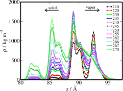
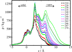
Figure 1: Density profiles of liquid-like molecules for the basal interface as measured relative to (a) the laboratory reference frame (b) the f-v surface and (c) the i-f surface. Since the liquid-like layer has finite thickness, the profiles vanish at the solid phase to the left and the vapor phase to the right of the z axis in these figures.

But despite its significance, and great experimental progress Furukawa et al. (1987); Dosch et al. (1996); Wei et al. (2001); Bluhm et al. (2002); Sadtchenko and Ewing (2002); Murata et al. (2016); Smit and Bakker (2017); Sánchez et al. (2017), the characterization of ice premelting has remained a longstanding matter of debate Li and Somorjai (2007); Michaelides and Slater (2017); Slater and Michaelides (2019). As the controversy regarding the film thickness could start to clarify with agreement between widely different experimental techniques Bluhm et al. (2002); Sadtchenko and Ewing (2002); Conde et al. (2008); Gelman Constantin et al. (2018); Mitsui and Aoki (2019), new and exciting observations have been made regarding the properties of the premelting film, both at Sánchez et al. (2017); Pickering et al. (2018); Qiu and Molinero (2018), and off ice/vapor coexistence Murata et al. (2016). Sanchez et al. performed a Sum Frequency Generation experiment (SFG) of the ice surface along the sublimation line and found evidence of a discrete bilayer melting transition Sánchez et al. (2017); Michaelides and Slater (2017). Off coexistence, experiments Murata et al. (2016) have found a discontinuous transition from a thin to a thick premelting film occurring at water-vapor supersaturation that is often known as frustrated complete wetting Shahidzadeh et al. (1998); Indekeu et al. (1999); Müller and MacDowell (2001); MacDowell and Müller (2005). An appealing interpretation is to view both phenomena as manifestations of layering effects and renormalization similar to those studied in past decades for simple model systems Weeks (1982); Huse (1984); Patrykiejew et al. (1990); Chernov and Mikheev (1988); Ball and Evans (1988); Evans (1992); Henderson (1994); Brader et al. (2001); Dijkstra and van Roij (2002). However, the evidence for layering is not without some controversy too as other studies also based on SFG suggest that bilayer melting occurs instead in a continuous fashion Smit and Bakker (2017). Interestingly, computer simulations show that the ice surface exhibits patches of premelted ice, whose size increases continuously as the temperature is increased, also consistent with a continuous build up of the premelting film Hudait et al. (2017); Pickering et al. (2018); Qiu and Molinero (2018).

Here we show that in the range between 230 to 270 K, the order parameter distributions of the main facets of ice exhibit the signature of two consecutive rounded layering transitions. This reconciles conflicting experimental and computer simulation studies of the equilibrium surface structure Sánchez et al. (2017); Smit and Bakker (2017); Hudait et al. (2017); Pickering et al. (2018); Qiu and Molinero (2018). Extrapolation of our results for the TIP4P/Ice model according to predictions of liquid state and renormalization theory indicate that a genuine first order phase transition occurs at supersaturation, consistent with experimental observations off-coexistence Murata et al. (2016). Our results provide a unified vision of the wetting behavior of premelting films on ice.

We use the TIP4P/Ice model, which exhibits a melting temperature of 272 K Abascal et al. (2005). To prepare the system in the solid/vapor coexistence region, we place an ice slab of either 1280 or 5120 molecules in vaccuum. Performing canonical Molecular Dynamics simulations Bussi et al. (2007) with GROMACS, the system attains two phase coexistence in a few nanoseconds and an equilibrated premelting film is formed spontaneously Conde et al. (2008); Benet et al. (2016); Kling et al. (2018); Llombart et al. (2019) (Supplementary Material). Previously, computer simulation evidence for a layering transition of the TIP4P/Ice model has been discussed in terms of the density profile $\rho(z)$ of the H₂O molecules as a function of the perpendicular distance, $z$ to the interface Sánchez et al. (2017). A more detailed description of layering phenomena in terms of density profiles is afforded by identifying liquid-like and solid-like environments Lechner and Dellago (2008); Nguyen and Molinero (2015). Using the $\bar{q}_{6}$ order parameter Lechner and Dellago (2008) allows us to plot the density of liquid-like and solid-like molecules, and identify features that are specific to the premelting layer Benet et al. (2016, 2019); Llombart et al. (2019).

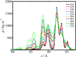
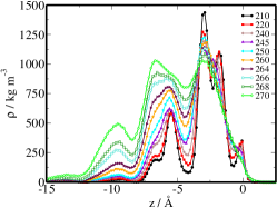
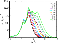
Figure 1: Density profiles of liquid-like molecules for the primary prism interface as measured relative to (a) the laboratory reference frame (b) the f-v surface and (c) the i-f surface.

The density profile of liquid-like molecules at the $\{0001\}$ face (or basal face) can be seen in Fig. 1(a). At low temperatures, the profile is highly structured, with the main peaks separated by about 3.5 Å, a value very close to the preferred lattice spacing of the underlying solid. This, together with the bilayer structure apparent as a double peak is suggestive of a rather ordered liquid-like environment. As temperature rises, the profiles transform in a continuous manner up to about 267 K. At this temperature a qualitative change is observed, as the outermost maxima and minima of the density profile disappear via an inflection point, leaving the profile with a monotonic decay into the vapor phase.

In fact, the strong stratification of the liquid-like profile is caused to a great extent by the structure of the underlying ice lattice. To show this, we describe the premelting liquid layer in terms of two bounding surfaces separating the quasi-liquid (fluid) film from bulk ice and bulk vapor Benet et al. (2016, 2019); Llombart et al. (2019). For points ${\bf x}$ along a flat reference plane, we calculate an ice-fluid (i-f) surface as the loci, $z_{\rm i-f}({\bf x})$ of the outermost solid-like molecules. Likewise, we calculate a fluid-vapor (f-v) surface, as the loci, $z_{\rm f-v}({\bf x})$ of the outermost liquid-like molecules (see Supplementary Material). An intrinsic density profile relative to the local f-v interface can then be determined as the density of atoms at a distance $z-z_{\rm f-v}({\bf x})$. The picture that emerges [Fig. 1(b)] shows a much less layered structure, confirming that the strong stratification of $\rho(z)$ shown in Fig. 1(a) is largely the result of structural correlations conveyed by the solid phase. The profile evolves continuously up to 264 K, with the outermost minimum and maximum again disappearing across an inflection point at about $z-z_{\rm f-v}({\bf x})=-2.2$ Å, as the decay of the density profile towards the vapor phase takes the monotonic form characteristic of a liquid-vapor interface.

The same insight can be found by plotting the intrinsic density profile of liquid-like molecules as measured relative to the fluctuating i-f surface [Fig. 1(c)], which is again less stratified than the absolute density profile. This profile also evolves in a rather continuous fashion, but, surprisingly, it does not show any particular signature of layering between 265 and 270 K as observed previously. Rather, in this case one notices the appearance of a maximum at about 6.7 Å which occurs via an inflection point between 230 and 235 K.

Whilst the details of the liquid-like density profiles at the prism facet $\{10\overline{1}0\}$ are very different, the main features observed at the basal facet are also found here, with intrinsic density profiles that are again very much rounded relative to the strongly stratified absolute density profile. A close inspection shows inflection points appear between 265 and 270 K and between 240 and 250 K (Supplementary Material).

In order to clarify the process of bilayer melting further, we need to resort to a more illuminating order parameter than the density profiles of liquid-like molecules. Based on the intrinsic i-f and f-v surfaces, we can define an instantaneous local film thickness as $\hat{h}({\bf x})=z_{\rm f-v}({\bf x})-z_{\rm i-f}({\bf x})$. We exploit this local parameter to calculate the mean film thickness $h$ after lateral and canonical averaging over the simulation run.

Fig. 2 depicts the results obtained for the basal plane. The film thickness grows from about one molecular layer at $T$=210 K, to about three molecular layers at $T$=270 K in a continuous fashion, with no clear evidence of a first order layering transition. Results obtained recently for the monoatomic water model (mW) show a similar trend but appear smoother as they are sampled in the grand canonical ensemble, which allows for larger film thickness fluctuations Pickering et al. (2018); Qiu and Molinero (2018). We provide a full thermodynamic characterization of wetting properties by calculating the disjoining pressure of the film, $\Pi(h)=-dg(h)/dh$, where $g(h)$ is the binding potential, which accounts for the pressure difference between the adsorbed liquid film and the bulk vapor of equal chemical potential, i.e. Derjaguin (1987); Henderson (2005); Benet et al. (2014):

$$\Pi(h)=p_{v}(\mu,T)-p_{l}(\mu,T).$$ (1)

In practice, $\Pi(h)$ is to an adsorbed liquid film as the Laplace pressure is to a liquid droplet. In particular, the vapor pressure of an ideal gas in equilibrium with a film of thickness $h$ is given in a manner analogous to the Kelvin-Laplace equation as $p_{v}=p_{v,w}e^{-\beta\Pi(h)/\rho_{w}}$, where $p_{v,w}$ is the saturated vapor pressure over water, $\rho_{w}$ is the bulk liquid density at coexistence and $\beta=(k_{B}T)^{-1}$. An equilibrium film thickness for water adsorbed at the ice/vapor interface can be meaningfully defined only along the sublimation line, where the vapor pressure equals the saturated vapor pressure over ice, $p_{v,i}$. Accordingly, the above equation becomes $p_{v,i}=p_{v,w}e^{-\beta\Pi(h)/\rho_{w}}$. It follows that using accurate coexistence vapor pressures, and the corresponding equilibrium film thickness $h(T)$ along the sublimation line, we can readily determine $\Pi(h)$ (Supplementary Material). The significance of this result can be hardly overemphasized. By exploiting the data $h(T)$ at solid/vapor coexistence, we can now determine the film height of the premelting film at arbitrary temperature and pressure, by merely solving Eq. (1) for $h$ Sibley et al. . This is a required input in theories of premelting Kuroda and Lacmann (1982); Nenow and Trayanov (1986); Wettlaufer (2019).

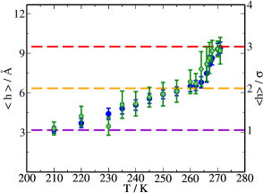
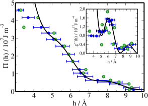
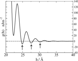
Figure 2: Film thickness (a), disjoining pressure (b), and interface potential (c) for the basal facet. Results are shown for two system sizes with $n_{x}\times n_{y}=5120$ (blue filled circles) and $n_{x}\times n_{y}=1280$ (green hollow circles) molecules. (a) The dashed lines indicate discrete film heights in units of the molecular diameter. (b) The lines are a fit of Eq. (2) to the blue symbols for $h>4.0$ Å. The insets show inverse surface susceptibilities as obtained from numerical deriviatives (symbols) and from analytical derivatives of the fits (lines). Error bars are shown here only for the system fitted to Eq. (2). Panel (c) shows the decay of the interface potential at intermediate distances as extrapolated from the fit to Eq. (2). Arrows indicate states that can transition at supersaturation, i.e. to frustrated complete wetting states.

Results for the basal surface are shown in Fig. 2. The disjoining pressure curve measured up to $h=10$ Å  exhibits a monotonic behavior, but with a clear damped oscillatory decay at positive disjoining pressure. In contrast, a system exhibiting first order layering transitions exhibits sinusoidal oscillations in mean field, or alternatively, an equal areas Maxwell construction with a segment of zero slope beyond mean field. We confirm the presence of the oscillatory behavior from plots of the derivative (obtained numerically) – see inset. Maxima of the inverse susceptibility, $\chi_{\parallel}^{-1}=d^{2}g/dh^{2}$, which characterizes parallel correlations, indicate enhanced stability at preferred film thicknesses of $h=6$ Å for the basal plane and at $h=5.4$ Å for the prism plane (Supplementary Material), but this is not a sufficient criteria for a thermodynamic phase transition. Thus, it appears that at a mean field level there could be layering which is washed away upon renormalization to larger length scales, as suggested from the study of capillary wave fluctuations Chernov and Mikheev (1988); Henderson (1994).

Liquid state theory provides an expansion for the renormalized interface potential $g(h)$ of a premelting film dominated by short range structural forces. To leading order in $h$, this gives:

$$g_{R}(h)=A_{2}e^{-\kappa h}-A_{1}e^{-\kappa_{R}h}\cos(k_{z,R}h),$$ (2)

where the amplitudes $A_{1}$ and $A_{2}$ depend on $T$, while $\kappa$ and $\kappa_{R}$ are inverse length scales that characterize the decay of the pair correlations in the liquid. Their values are renormalized from those one would expect on the basis of mean field theory, so that e.g. $k_{z,R}<k_{z}$, where $k_{z}$ is the wavenumber corresponding to the maximum of the bulk liquid structure factor Chernov and Mikheev (1988); Evans (1992); Henderson (1994); Evans et al. (1994); Hughes et al. (2017).

This result is an asymptotic form, and is not expected to hold for small thicknesses of barely one molecular diameter. However, a fit of $\Pi(h)=-dg_{R}(h)/dh$ as predicted by Eq. (2) for all $h>4.0$ Å  exhibits an excellent agreement with simulation data. Moreover, from the fitting parameters we can determine the wetting behavior at short and intermediate $h$. For the basal facet ($\kappa=0.61$ Å^-1, $\kappa_{R}=0.43$ Å^-1 and $k_{z,R}=2.36$ Å^-1) we find $\kappa_{R}<\kappa$, so that $g(h)$ exhibits an absolute minima at intermediate distances. This implies incomplete wetting of the premelting film, as expected for facets below the roughening temperature of the solid/melt interface Chernov and Mikheev (1988); Evans (1992); Henderson (1994). For the prism plane ($\kappa=0.62$ Å^-1, $\kappa_{R}=0.90$ Å^-1 and $k_{z,R}=3.14$ Å^-1) we find in contrast that $\kappa_{R}>\kappa$, so that $g(h)$ exhibits a monotonous decay. This leads to complete wetting of the premelting film as a result of a fluctuation dominated wetting transition Chernov and Mikheev (1988). Of course, for very large $h$ the decay rate of $\kappa_{R}$ is not expected to depend on the crystal facet. However, for intermediate values of $h$ of interest here the decay need not be exactly the same, since the renormalized quantities depend on details of the interface potential at short range. In practice, at sufficiently large distance van der Waals forces with algebraic decay will favor incomplete wetting irrespective of the surface plane involved Elbaum and Schick (1991).

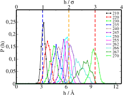
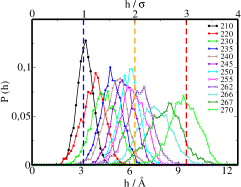
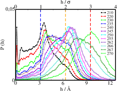
Figure 3: System size analysis of thickness distributions at the basal plane. (a) probability distribution of the global film thickness, $h$. (b) probability distribution of the partial film thickness $h_{1/4}$. (c) probability distribution of the local order parameter $h({\bf x})$. Dashed vertical lines show the film thickness in units of the molecular diameter. Results are shown for temperatures in the range from $T$=210 K to $T$=271 K, with color code as indicated on the figure.

To clarify whether the layering is consistent with either a continuous or a first order phase transition, we perform a block analysis of the film thickness distributions Binder (1981); Landau and Binder (2000), and plot the probability distribution of film thicknesses averaged over lateral areas of increasing size. We consider $h({\bf x})$, which accounts for a lateral size of two unit cells; $h_{1/4}$, which accounts for an average over a quarter of the full system, and $h$, an average over the full system size. The results are presented in Fig. 3.

For the local order parameter $h({\bf x})$, we find rather broad distributions, which span as much as $9$ Å, i.e., $\approx 3$ molecular diameters. In the event of a first order phase transition, broad distributions found in small systems become bimodal, with two sharp peaks separated by a gap of increasingly smaller probability as the system size grows. Contrary to this scenario, the block analysis performed over distributions of $h_{1/4}$ and $h$, shows that no signs of bimodality persist in any of these distributions, the peaks appear to sharpen significantly, and the gap between two and three layers is filled with unimodal distributions. However, the distributions corresponding to fully formed layers are clearly much sharper, while those corresponding to distances in between remain broader, i.e. exhibit enhanced fluctuations. This scenario resembles that of a continuous phase transition in a finite system Binder (1981); Landau and Binder (2000), but our block analysis does not show evidence of singular behavior. Accordingly, it appears that the system is traversing the prolongation of a first order phase transition beyond the critical point, across a continuous and non-singular transition. This explains why SFG experiments, which probe a local order parameter, can detect distinct spectral changes of the local environment as temperature is raised.

Indeed, an analysis of average mean square fluctuations and higher moments (Supplementary Material) reveals the signature of two rounded layering transitions on the basal plane, first, from one to two bilayers, at about $T$=235 K, then from two to three bilayers at $T$=267 K. These transitions very much correlate with the inflection points observed previously in the density profiles. The latter is consistent with results by Sanchez et al. for the TIP4P/Ice model, which bracketed the bilayer melting between 260 and 270 K Sánchez et al. (2017). Hints of an inflection in the premelting film thickness that could be consistent with the same phenomena are also observable in the mW model at about 260 K Pickering et al. (2018); Qiu and Molinero (2018). For the primary prism plane (Supplementary Material) the results are similar and reveal the presence of two rounded transitions at about 250 K and 267 K, as suggested from the study of inflection points in the density profile. The transitions at 235 K and 250 K observed for basal and prism planes correlate with the onset of surface mobility reported recently for the same model Kling et al. (2018).

Interestingly, the distance between maxima of the global order parameter distribution increases with film height. For the basal plane the three maxima are separated by 2.9 and 3.4 Å, respectively. For the prism plane, the separation is 2.3, 2.7 and 3.6 Å, respectively. This is again consistent with the renormalization scenario, since we expect the renormalization of $k_{z}$ to be more significant as the distance from the substrate increases. Thus, it might be possible that true first order transitions occur for large $h$ between adjacent minima that are several molecular diameters apart as a result of renormalization. This view provides an explanation for the experimental observation of frustrated complete wetting in confocal microscopy experiments Murata et al. (2016).

In summary, we document the existence of rounded layering transitions with enhanced fluctuations at 235 and 267 K for the basal interface and at 250 and 267 K for the prism interface. We conjecture that the continuation of a line of true first order layering transitions beyond the layering critical point could intersect the sublimation line and explain the enhanced fluctuations observed here. This reconciles conflicting interpretations of layering on the ice surface Sánchez et al. (2017); Smit and Bakker (2017); Qiu and Molinero (2018), and opens exciting new avenues for experimental verification.

Supporting Information for

Rounded layering transitions on the surface of ice
by
Pablo Llombart^†,‡, Eva G. Noya^‡, David N. Sibley^§, Andrew J. Archer^§ and Luis G. MacDowell^†

^†Departamento de Química-Física (Unidad de I+D+i Asociada al CSIC), Facultad de Ciencias Químicas, Universidad Complutense de Madrid, 28040 Madrid, Spain,
^‡Instituto de Química Física Rocasolano, CSIC, Calle Serrano 119, 28006 Madrid, Spain and
^§Department of Mathematical Sciences, Loughborough University, Loughborough LE11 3TU, United Kingdom.

Results for the Primary Prism facet

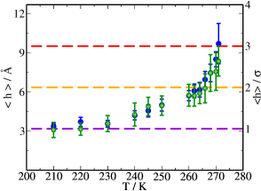
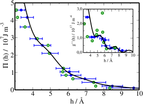
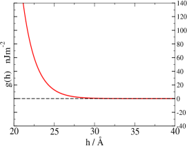
Figure 2: Film thickness (a), disjoining pressure (b), and interface potential (c) for the primary prism facet. Results are shown for two system sizes with $n_{x}\times n_{y}=5120$ (blue filled circles) and $n_{x}\times n_{y}=1280$ (green hollow circles) molecules. (a) The dashed lines indicate discrete film heights in units of the molecular diameter. (b) The lines are a fit to Eq. (2). The insets show inverse surface susceptibilities as obtained from numerical derivatives (symbols) and from analytical derivatives of the fits (lines). Error bars here are shown only for the data fitted to Eq. (2). Panel (c) shows the decay of the interface potential at intermediate distances as extrapolated from the fit to Eq. (2). The decay of the interface potential here is monotonic.

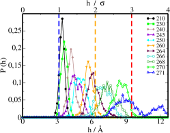
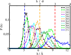
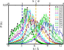
Figure 3: System size analysis of thickness distributions at the primary prism plane. Panels (a) probability distribution of the global film thickness, $h$. (b) probability distribution of the partial film thickness $h_{1/4}$. (c) probability distribution of the local order parameter $h({\bf x})$. Dashed vertical lines show the film thickness in units of the molecular diameter. Results are shown for temperatures in the range from $T$=210 K to $T$=271 K, with color code as indicated on the figure.

Disjoining pressure

The three phases involved are the ice substrate (i), the water film (f) and the vapor (v). The discussion below is rather general, so here we refer to the three phases as solid (s), liquid (l) and vapor (v). Consider an inert substrate in contact with a stable vapor phase at fixed temperature, $T$. It is convenient to study the system in the grand canonical ensemble, where the chemical potential $\mu$ is fixed at the outset, and one assumes the adsorbed layer can grow to its equilibrium value while the vapor pressure remains constant. By this device, one fixes the vapor pressure of the system to the corresponding bulk vapor pressure $p_{v}(T,\mu)$ at the selected chemical potential. The corresponding bulk liquid phase of equal temperature and chemical potential has a bulk pressure, $p_{l}(T,\mu)$.

Consider that $(T,\mu)$ are such that the bulk vapor phase is more stable than the bulk liquid phase. For a column of height $h$ filled by bulk vapor, the free energy per unit surface is given by $\omega_{v}(T,\mu)=-p_{v}(T,\mu)h$. Similarly, for an equivalent column filled with bulk liquid, the corresponding free energy is given as $\omega_{v}(T,\mu)=-p_{l}(T,\mu)h$. Below the bulk liquid-vapor coexistence, it always holds $p_{v}(T,\mu)>p_{l}(T,\mu)$, such that the vapor phase has the lowest free energy and is the preferred phase. The free energy difference per unit surface area between a liquid filled and vapor filled column is given as $\Delta\omega(T,\mu)=\Delta p_{lv}(T,\mu)h$, where $\Delta p_{lv}(\mu,T)=-[p_{l}(T,\mu)-p_{v}(T,\mu)]$ is the familiar Laplace pressure difference used in classical nucleation theory.

If the column of bulk phase is moved next to the substrate, however, a finite amount of liquid phase is usually stabilized, even if the thermodynamic fields have been selected such that the bulk vapor phase is most stable. The interface potential, $g(h)$ accounts for the free energy gained by the liquid phase in contact with the substrate.

The excess free energy of the liquid film of thickness $h$ adsorbed on a substrate is given as:

$$\omega(h;T,\mu)=\gamma_{sl}+\gamma_{lv}+g(h;T)-\Delta p_{lv}(T,\mu)h,$$ (3)

Here, $-\Delta p(T,\mu)h$, is the bulk free energy cost to replace the bulk vapor by a liquid film, $g(h)$ accounts for the free energy gained by the bulk liquid phase due to the influence of the substrate at liquid-vapor coexistence, while $\gamma_{sl}$ and $\gamma_{lv}$ are the solid-liquid and liquid-vapor interfacial tensions, respectively.

The condition of equilibrium for the adsorbed film at constant $T,\mu$ is:

$$\frac{d\omega(h;T,\mu)}{dh}=0.$$ (4)

This provides the celebrated Derjaguin equation Derjaguin (1987); Henderson (2005); Benet et al. (2014):

$$\Pi(h;T)=-\Delta p_{lv}(T,\mu),$$ (5)

where $\Pi(h;T)$ is the disjoining pressure, defined as $\Pi(h;T)=-dg(h;T)/dh$.

In standard applications for adsorbed liquids on an inert substrate, one usually measures an adsorption isotherm, i.e., $h=h(T,\mu)$, at fixed temperature, while changing the chemical potential (or vapor pressure). The disjoining pressure is calculated by matching the measured equilibrium film thickness at increasing vapor pressure with the corresponding pressure difference, $\Delta p_{lv}(T,\mu)$ Benet et al. (2014).

For a premelting film, the situation is far more complicated, because adsorption from the vapor phase takes place on a solid substrate that is found at phase coexistence with the vapor. i.e., the vapor-substrate equilibrium states only exist along the sublimation or solid-vapor coexistence line, corresponding to a fixed chemical potential $\mu_{sv}=\mu_{sv}(T)$. Therefore, at fixed temperature one cannot meaningfully collect equilibrium film thicknesses $h$ as a function of vapor pressure, since equilibrium is achieved only at exactly the solid-vapor coexistence pressure, $p_{sv}(T,\mu_{sv}(T))$.

The way out is to relax the constraint of fixed temperature. Instead, we collect the equilibrium film thicknesses $h(T)|_{sv}=h(T,\mu_{sv})$ along the sublimation line, where the notation $X(T)|_{sv}$ denotes a property $X(T)$ measured at the chemical potential $\mu_{sv}=\mu_{sv}(T)$ of solid/vapor coexistence. These film thicknesses are then mapped onto $\Delta p_{lv}(T)|_{sv}$, i.e., the pressure difference between bulk liquid and vapor phases measured at the solid-vapor coexistence chemical potential.

Taking into account that the temperature dependence of $g(h;T)$ and $\Pi(h;T)$ is small, one can get a single disjoining pressure master curve $\Pi(h)$ from these data. Accordingly, the function $\Pi(h)$ is obtained in three steps:

• Measure the equilibrium film thickness $h(T)|_{sv}$ along the sublimation line. In practice, this is readily done by direct coexistence $NVT$ simulations. Placing a slab of ice in contact with vacuum at a temperature $T$, the system gradually equilibrates and attains solid-vapor coexistence. Accordingly, once the system is well equilibrated, the vapor phase is automatically selected to exhibit the sublimation vapor pressure without a priori knowledge of the corresponding chemical potential. In between the almost empty vapor phase and the bulk ice phase, a premelting liquid film is formed in a few nanoseconds. The equilibrium film thickness that is obtained corresponds to the desired curve, $h(T)|_{sv}$.

• Calculate the Laplace pressure difference between bulk liquid and vapor phases at the solid-vapor coexistence chemical potential, $\Delta p_{lv}(T)|_{sv}$. Below we show that this pressure difference can be related to the liquid-vapor and solid-vapor coexistence pressures. Using the Clapeyron equation the coexistence pressures may be obtained from triple point data only. In practice, we assume an ideal gas for the vapor phase, and obtain accurate approximations for the solid and liquid properties at the triple point from $NpT$ simulations at zero pressure (see below).

• Map the results of $h(T)|_{sv}$ onto $\Delta p_{lv}(T)|_{sv}$ to obtain the disjoining pressure curve from Eq. (5) as:

  $$\Pi(h(T)|_{sv})=-\Delta p_{lv}(T)|_{sv}$$ (6)

Laplace pressure difference along the sublimation line

In order to evaluate the disjoining pressure, we need to know the Laplace pressure difference $\Delta p_{lv}(T)|_{sv}$ between the bulk liquid and vapor phases at equal temperature and chemical potential, for selected chemical potentials along the sublimation line.

It turns out that this calculation can be performed following thermodynamic calculations that are familiar in classical nucleation theory.

Here, we are interested in calculating the pressure difference $\Delta p_{lv}(T)=p_{l}(T,\mu)-p_{v}(T,\mu)$ between an adsorbed liquid phase and a reservoir vapor phase with chemical potential $\mu$. Using the Gibbs-Duhem equation, $dp=\rho\,d\mu$, with $\rho$, the bulk density, we write:

$$d(p_{l}-p_{v})=(\rho_{l}-\rho_{v})d\mu.$$ (7)

Since the vapor density is much smaller than the liquid density, we assume $\rho_{l}-\rho_{v}\approx\rho_{l}$. Furthermore, since the liquid is effectively incompressible for the small chemical potential changes that concern us here, we assume constant liquid density and integrate the above equation from the liquid-vapor coexistence chemical potential to arbitrary chemical potential at fixed temperature, yielding:

$$p_{l}(T,\mu)-p_{v}(T,\mu)=\rho_{l}(\mu-\mu_{lv}),$$ (8)

where $\mu_{lv}$ is the chemical potential at liquid-vapor coexistence and we have taken into account that $p_{l}(T,\mu_{lv})-p_{v}(T,\mu_{lv})=0$.

Now, assuming the vapor phase is an ideal gas, we obtain:

$$p_{l}(T,\mu)-p_{v}(T,\mu)=\rho_{l}RT\ln p/p_{lv}(T),$$ (9)

where $p(T)_{lv}$ is the liquid-vapor coexistence pressure and $p$ is the pressure of the vapor phase with arbitrary chemical potential $\mu$. This is the result used in classical nucleation theory for the pressure difference of a liquid nucleus in equilibrium with the vapor reservoir phase. Here we use the same equation for the adsorbed liquid layer in equilibrium with a vapor reservoir phase.

It follows immediately that the sought Laplace pressure difference along the sublimation line, where $p=p_{sv}$ by definition, is given as:

$$\Delta p_{lv}|_{sv}=\rho_{l}RT\ln\frac{p_{sv}(T)}{p_{lv}(T)}.$$ (10)

Therefore, $\Delta p_{lv}(T)|_{sv}$ may be calculated from knowledge of the vapor pressures along the condensation and sublimation lines.

In order to obtain $p_{sv}(T)$ and $p_{lv}(T)$, we invoke the Clausius equation for the coexistence pressure, $p_{\alpha v}$ of an arbitrary phase, $\alpha$, with the bulk vapor:

$$\frac{dp_{\alpha v}}{dT}=\frac{\Delta H_{\alpha v}}{T\Delta V_{\alpha v}},$$ (11)

where $\Delta H_{\alpha v}$ and $\Delta V_{\alpha v}$ are the enthalpy and volume change of transition. For water below the triple point, the volume of the vapor phase is more than 1000 times larger than that of either liquid or solid phases, so we can approximate $\Delta V_{\alpha v}$ to the volume of the vapor phase $V_{v}$, and further replace this with the ideal gas equation, leading to the Clausius-Clapeyron result:

$$\frac{dp_{\alpha v}}{p}=\frac{\Delta H_{\alpha v}}{RT^{2}}dT.$$ (12)

In many applications, this equation is integrated under the assumption of constant $\Delta H_{\alpha v}$. We improve this approximation by expanding the enthalpy of phase change to first order about the triple point:

$$\Delta H=\Delta H_{t}+\Delta C_{p,t}(T-T_{t}),$$ (13)

where $\Delta C_{p,t}$ is the difference of heat capacities between the corresponding condensed phase and the coexisting vapor phase at the triple point. This then finally yields:

$$\ln(p_{\alpha v}(T)/p_{t})=\frac{\Delta H_{t}-\Delta C_{p,t}T_{t}}{R}\left[1/T_{t}-1/T\right]+\frac{\Delta C_{p,t}}{R}\ln(T/T_{t}),$$ (14)

where here $\Delta H_{t}$ is the enthalpy of phase change, and the subindex $\alpha$ corresponds to either liquid or solid phases.

In order to evaluate this equation, we calculated enthalpies and heat capacities for the TIP4P/Ice model at the triple point temperature $T_{t}=272$ K and zero pressure. Results for the required properties may be found in Table 1.

$H^{iv}_{t}$ / KJ mol-1	$H^{wv}_{t}$ / KJ mol-1	$C_{p,t}^{i}$/ J mol-1K-1	$C_{p,t}^{w}$ / J mol-1K-1
-61.03	-55.64	65.60	107.26

Table 1: Thermophysical properties of the TIP4P$/$Ice model at the triple point $T_{t}=272$ K, required for the determination of the sublimation and condensation pressures.

I Moments of the distributions and rounded transitions

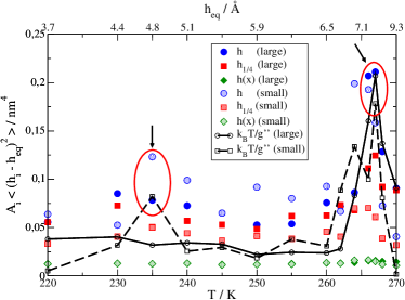
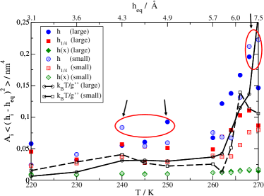
Figure 4: Scaled mean squared fluctuations of the film thickness. Results are shown for the large (filled symbols) and small (hollow symbols) systems. The latter is $2\times 2$ smaller than the former. The figure shows moments for fluctuations of the global film thickness, $h$ (circles), for subsystems with size 1/4, $h_{1/4}$ (squares) and for the local thickness $h(x)$ (diamonds). Black lines show the scaled mean squared fluctuations as given by the right hand side of Eq. (17), with $\chi_{\parallel}^{-1}$ estimated from the second derivatives of the interface potential, $g^{\prime\prime}(h)$. Results are shown for large (full lines) and small (dashed lines) systems. Arrows point roughly to the location of the maxima of mean squared fluctuations.

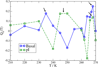
Figure 5: Binder cumulants of the global order parameter for the large (blue circles) and small (green squares) systems. The arrows point to maxima of the cumulants, which serves to roughly locate the transitions.

Since the probability distributions of the order parameter in Fig. 3 of the main manuscript and Fig. 3 of the supplementary material are normalized to unity, a rough estimate of the mean squared amplitude of the fluctuations can be made from the height of the maxima of the distributions. From these plots, one finds that the maxima corresponding to partially filled layers are less pronounced than those corresponding to filled layers. Accordingly, the fluctuations are larger for the former and we can estimate the loci of the rounded transitions from the distribution with largest fluctuations. By visual inspection, this suggests rounded transitions at about 235 K and 266 K for the basal face, and at about 250 K and 266 K for the prism face. Of course, because of the limited statistics, the finite size transitions are given with an error of $\pm 2$ K at least.

A quantitative analysis requires consideration of the probability distribution in more detail. In our simulations, the system is found at solid vapor coexistence by construction. The chemical potential is therefore fixed exactly at coexistence. Furthermore, the system features a large bulk phase, which roughly serves as a particle and heat reservoir for the premelting film. Therefore, we may consider the premelting film as effective being treated grand canonically. For a system away from the line of layering transitions, the surface free energy in Eq. (3) at the imposed constant temperature and chemical potential can be expanded to quadratic order as:

$$\omega(h;T,\mu)=\omega(h_{eq},T,\mu)+\frac{1}{2}\chi_{\parallel}^{-1}(h-h_{eq})^{2},$$ (15)

where $h_{eq}$ is the equilibrium film thickness, and the susceptibility has been defined as $\chi_{\parallel}^{-1}=g^{\prime\prime}(h_{eq})$. The surface free energy is related to the probability distribution as $A\omega(h;T,\mu)=-k_{B}T\ln P(h;T,\mu)$, where $A$ is the lateral area. Accordingly, the probability distribution of the order parameter is (c.f. Ref.Binder (1981); Landau and Binder (2000)):

$$P(h)=Ce^{-\frac{1}{2}\beta A\chi_{\parallel}^{-1}(h-h_{eq})^{2}},$$ (16)

with $C$ a normalization constant. This has a Gaussian form, so the mean squared fluctuations of $h$ in a system with lateral size $A$ will obey:

$$A\langle(h-h_{eq})^{2}\rangle=k_{B}T/\chi_{\parallel}^{-1}.$$ (17)

Fig. 4 shows the scaled mean squared fluctuations, which, from Eq. (17), should become constant, independent of the system size in the thermodynamic limit for non-singular transitions. From the figure we find this holds indeed already for the limited system sizes studied here. Despite a considerable scatter of the simulation data, maxima of the fluctuations for a fixed system size are observed roughly as estimated from visual inspection of the distributions. As an additional consistency check, we also show as a black line the expectation for the scaled mean squared fluctuations as obtained from the inverse susceptibilities of the interface potential depicted in the inset of Fig. 2(b) of the main manuscript and this document. The agreement seems fairly good, considering the limited statistics and finite size effects.

In order to further analyse the rounded transitions, it is convenient to consider the Binder cumulant of the distributions, which is given as Landau and Binder (2000):

$$Q_{h}=1-\frac{1}{3}\frac{\langle(h-h_{eq})^{4}\rangle}{\langle(h-h_{eq})^{2}\rangle^{2}}.$$ (18)

For a system away from a critical point, the distributions are Gaussian, and $Q_{h}$ is approximately zero. Close to a phase transition, however, $Q_{h}$ is expected to approach $2/3$ in the thermodynamic limit.

Fig. 5 shows plots of $Q_{h}$ as obtained from the moments of the global order parameter of the largest system. Results for the remaining order parameters are similar, but are quite noisy and do not afford a study of system size effects. From the plot, it can be clearly seen that most values of $Q_{h}$ fluctuate about 0, the result expected for a disordered phase. The location of rounded transitions is visible in the maxima of the cumulants, as indicated by the arrows. The maxima are roughly coincident with the expected location as revealed from the analysis of the mean squared fluctuations in Fig.4 and the inflection points of density profiles. However, their value is far smaller than 2/3, the expected result for a critical point, and lend further support to our claim of rounded layering transitions.

Density profiles for solid-like molecules

Density profiles for solid-like molecules for a selected range of temperatures are shown in Fig. 6.

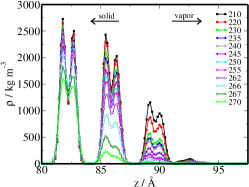
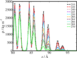
Figure 6: Density profiles for solid-like molecules as a function of temperature. (a) Basal (b) Prism planes.

Parameters for the fit to the interface potential

The coefficients of the fit for the interfacial potential form given in Eq. (2) in the main text are displayed in Table 2.

face	fit	A1/$J\,m^{-2}$	A2/$J\,m^{-2}$	$\kappa\cdot$Å	$\kappa_{R}$ $\cdot$Å	$k_{z,R}\cdot$Å	$\theta$/rad
Basal	mf	0.1064	0.00100	0.6170	$2\kappa$	2.269	10.919
Basal	R	0.1070	0.00161	0.6102	0.429	2.360	10.323
pI	mf	0.0662	0.000148	0.6078	$2\kappa$	3.149	7.716
pI	R	0.0701	0.00379	0.6206	0.900	3.144	7.796

Table 2: Parameters for the fit of simulated disjoining pressures to the model interface potential in Eq. (2) for basal and prism planes. Results for the constrained fit with $2\kappa=\kappa_{R}$ are also shown.

Computer Simulations

At low saturation, ice crystals grow as hexagonal prisms, exhibiting two well defined facets. The base of the prism corresponds to the $\{0001\}$ crystal facets, and is also known as the basal facet. The sides of the prism correspond to $\{10\overline{1}0\}$ facets, and are known as the prism facets. For further details on the preparation of the initial configuration, we refer to our previous work, Ref.Benet et al. (2016, 2019); Llombart et al. (2019)

Our simulations are carried out with the TIP4P/Ice model Abascal et al. (2005). Phase space sampling is performed using Molecular Dynamics with the GROMACS package. Trajectories are evolved using the Leap-frog algorithm, with a time step of 3 fs. Bond and angle constraints are applied using the LINCS algorithm. Trajectories are thermostated in the NVT ensemble using the velocity rescale algorithm Bussi et al. (2007). Lennard-Jones interactions are truncated at a distance of 9 Å. Electrostatic interactions are evaluated using Particle Mesh Ewald, with the real space contribution truncated also at 9 Å. The reciprocal space term is evaluated over a total of $80\times 64\times 160$ vectors in the $x$, $y$, $z$ reciprocal directions, respectively. The charge structure factors were evaluated with a grid spacing of 0.1 nm and a fourth order interpolation scheme. For each temperature, we performed an $NpT$ simulation at 1 bar to obtain the corresponding equilibrium lattice parameters. The $NVT$ simulations that are then employed use equilibrated lattice parameters at that temperature. In order to prepare roughly square surfaces, we build a unit supercell of size $(2\times a)\times b\times c$, with $a$, $b$ and $c$, the unit cell parameters of a pseudo-orthorhombic cell of 8 molecules. Simulations are performed for two system sizes, a large system size, consisting of $8\times 8\times 5$ and a smaller one with $4\times 4\times 5$ unit supercell with 16 molecules each. More detailed information on the simulations may be found in our previous work Benet et al. (2016, 2019); Llombart et al. (2019).

Details of the system sizes studied may be found in Tables 3 and 4. Results for the film thickness may be found in Tables 5 and 6. Further details of the simulations may be found in Llombart et al. (2019).

Order parameter

In our study, we need to distinguish solid-like from liquid-like molecular environments in order to determine the premelting layer thickness and to locate the ice/water surface. For each water molecule, we perform a neighbor analysis and determine the $\bar{q}_{6}$ parameter, which is known to distinguish well solid and liquid molecules in bulk environments Lechner and Dellago (2008). All water molecules with $\bar{q}_{6}$ larger than a threshold value, $\bar{q}_{6}^{*}$, are classified as solid-like, while molecules with smaller $\bar{q}_{6}$ parameter are classified as liquid-like. In order to calculate the threshold value, we perform simulations of the bulk solid and liquid phases. From the distribution of $\bar{q}_{6}$ in each phase, we determine the value of $\bar{q}_{6}^{*}$ which produces the least amount of mislabeling. The threshold value is $\bar{q}_{6}^{*}\approx 0.35$ in the neighborhood of the triple point, but depends slightly on temperature. We refer to our recent work for further details and explicit results for the dependence of $\bar{q}_{6}^{*}$ on temperature Llombart et al. (2019).

An interesting alternative to the $\bar{q}_{6}$ parameter is the CHILL+ algorithm, which has been devised explicitly to discriminate solid-like environments different from hexagonal ice Ih Nguyen and Molinero (2015). In particular, the CHILL+ algorithm allows one to identify other ice crystal allotropes such as ice Ic, clathrate ice and interfacial ice Ih. In our previous work Llombart et al. (2019), we have shown that the $\bar{q}_{6}$ parameter essentially lumps all of these forms into the disordered liquid-like category. Therefore, our choice of order parameter essentially distinguishes the bulk ice Ih template from all other ice environments. The conventional application of CHILL+ is to label solid and liquid-like molecules in the the opposite extreme, i.e. to have the intermediate forms ice Ic, chlathrate ice and interfacial ice Ih lumped into the solid-like category, and have the liquid-like category for all remaining disordered forms. Fig. 7 display premelting film thicknesses as dictated by either of these two prescriptions. Starting from a temperature of about $T=240$ K, we find that either deffinitions differ essentially by a constant offset. Below this temperature, on the other hand, we find that both parameters are very similar. It follows that the first transition found in our work corresponds to an increase of undercoordinated ice forms. Surprisingly, both the $\bar{q}_{6}$ and CHILL+ recipes yield a close to monolayer thick disordered liquid layer at temperatures as low as 210 K. A detailed analysis of surface ice structure and coordination is left for future work.

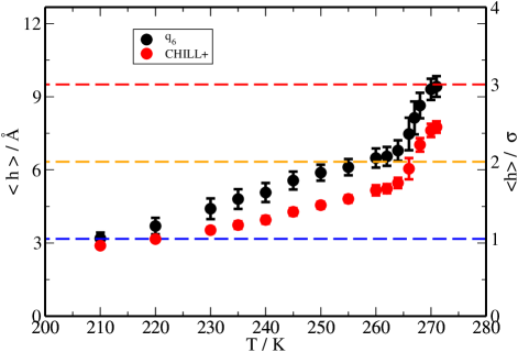
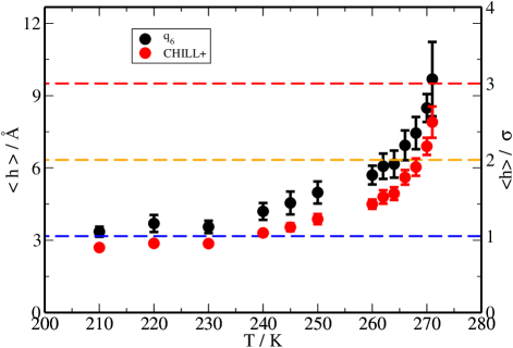
Figure 7: Premelting layer thickness measured using the $\bar{q}_{6}$ parameter as in this work (black), and with the CHILL+ parameter (red) for basal (left) and prism (right) facets.

Intrinsic surfaces

For each saved snapshot, we calculate the i-f and f-v intrinsic surfaces, meant to describe the local height of the premelting film at each point ${\bf x}$ on a reference plane parallel to the interface. First we analyze the local environment of each molecule in order to label them as liquid-like or solid-like with the $\bar{q}_{6}$ order parameter as described above Lechner and Dellago (2008). For a given point, ${\bf x}$, we calculate the i-f surface as the vertical position, $z_{\rm i-f}({\bf x})$ obtained from the average $z$ position of the four outermost solid-like atoms within one pseudo-orthorhombic unit cell of size $a\times b\times c$ about the point ${\bf x}$. Likewise, the f-v surface is calculated from the average $z$ position of the four outermost liquid-like molecules within an area of $3\sigma\times 3\sigma$ about ${\bf x}$, with $\sigma$ the Lennard-Jones range parameter of the TIP4P/Ice model. The procedure is illustrated in Fig. 8.

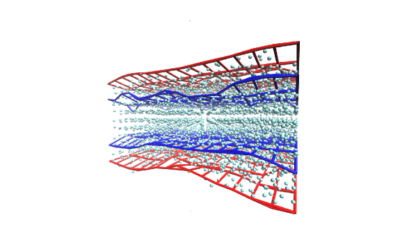
Figure 8: Sketch showing the i-f and f-v bounding surfaces that we employ to characterize the premelting film. The i-f surface is shown in blue and the f-v surface is shown in red.

System sizes studied

Detailed information on the system sizes studied are described in Tables III and IV.

Temperature / K	$N$ = 5120, $L_{x}\times L_{y}\times L_{z}$ / nm	$N$ = 1280, $L_{x}\times L_{y}\times L_{z}$ / nm
210	7.24541 $\times$ 6.27494 $\times$ 15.00000	3.62270 $\times$ 3.13747 $\times$ 15.00000
220	7.24868 $\times$ 6.27776 $\times$ 15.00000	3.62434 $\times$ 3.13888 $\times$ 15.00000
230	7.25247 $\times$ 6.28104 $\times$ 15.00000	3.62623 $\times$ 3.14052 $\times$ 15.00000
235	7.25427 $\times$ 6.28292 $\times$ 15.00000	3.62714 $\times$ 3.14146 $\times$ 15.00000
240	7.25609 $\times$ 6.28412 $\times$ 15.00000	3.62804 $\times$ 3.14206 $\times$ 15.00000
245	7.25780 $\times$ 6.28587 $\times$ 15.00000	3.62890 $\times$ 3.14294 $\times$ 15.00000
250	7.25949 $\times$ 6.28713 $\times$ 15.00000	3.62974 $\times$ 3.14356 $\times$ 15.00000
255	7.26152 $\times$ 6.28888 $\times$ 15.00000	3.63076 $\times$ 3.14444 $\times$ 15.00000
260	7.26350 $\times$ 6.29060 $\times$ 15.00000	3.63175 $\times$ 3.14530 $\times$ 15.00000
262	7.26419 $\times$ 6.29120 $\times$ 15.00000	3.63209 $\times$ 3.14560 $\times$ 15.00000
264	7.26488 $\times$ 6.29181 $\times$ 15.00000	3.63244 $\times$ 3.14590 $\times$ 15.00000
266	7.26558 $\times$ 6.29241 $\times$ 15.00000	3.63270 $\times$ 3.14620 $\times$ 15.00000
267	7.26586 $\times$ 6.29264 $\times$ 15.00000	3.63293 $\times$ 3.14632 $\times$ 15.00000
268	7.26628 $\times$ 6.29302 $\times$ 15.00000	3.63314 $\times$ 3.14651 $\times$ 15.00000
270	7.26698 $\times$ 6.29362 $\times$ 15.00000	3.63349 $\times$ 3.14681 $\times$ 15.00000
271	7.26731 $\times$ 6.29432 $\times$ 15.00000	3.63360 $\times$ 3.14716 $\times$ 15.00000

Table 3: Temperature and systems dimensions for the basal interface. The number of unit cells in $x$, $y$ and $z$ directions are $N_{x}=8$, $N_{y}=8$ and $N_{z}=5$ for the bigger system. The small system has half $(N/2)$ unit cells in the $x$ and $y$ directions and equal number of unit cells along $z$.

Temperature / K	$N$ = 5120, $L_{x}\times L_{y}\times L_{z}$ / nm	$N$ = 1280, $L_{x}\times L_{y}\times L_{z}$ / nm
210	7.24528 $\times$ 5.89679 $\times$ 15.00000	3.62270 $\times$ 2.94840 $\times$ 15.00000
220	7.24876 $\times$ 5.89961 $\times$ 15.00000	3.62434 $\times$ 2.94980 $\times$ 15.00000
230	7.25229 $\times$ 5.90249 $\times$ 15.00000	3.62623 $\times$ 2.95124 $\times$ 15.00000
240	7.25604 $\times$ 5.90554 $\times$ 15.00000	3.62804 $\times$ 2.95277 $\times$ 15.00000
245	7.25780 $\times$ 5.90697 $\times$ 15.00000	3.62890 $\times$ 2.95348 $\times$ 15.00000
250	7.25957 $\times$ 5.90841 $\times$ 15.00000	3.62974 $\times$ 2.95420 $\times$ 15.00000
260	7.26329 $\times$ 5.91143 $\times$ 15.00000	3.63175 $\times$ 2.95571 $\times$ 15.00000
262	7.26405 $\times$ 5.91205 $\times$ 15.00000	3.63209 $\times$ 2.95602 $\times$ 15.00000
264	7.26480 $\times$ 5.91267 $\times$ 15.00000	3.63244 $\times$ 2.95633 $\times$ 15.00000
266	7.26556 $\times$ 5.91328 $\times$ 15.00000	3.63270 $\times$ 2.95664 $\times$ 15.00000
268	7.26631 $\times$ 5.91389 $\times$ 15.00000	3.63314 $\times$ 2.95694 $\times$ 15.00000
270	7.26707 $\times$ 5.91452 $\times$ 15.00000	3.63349 $\times$ 2.95726 $\times$ 15.00000
271	7.26729 $\times$ 5.91470 $\times$ 15.00000	3.63360 $\times$ 2.95735 $\times$ 15.00000

Table 4: Temperature and systems dimensions for the prism face. The number of unit cells is as for the basal face listed in the caption of Table 3

Film thickness for two different system sizes

The film thicknesses displayed in Figures in the text are shown in tabulated form in Tables V and VI.

Temperature / K	$\langle h\rangle$ / Å(Area = 1)	$\langle h\rangle$ / Å(Area = $\frac{1}{4}$)
210	3.18	3.29
220	3.69	4.23
230	4.40	3.46
235	4.80	5.10
240	5.07	5.17
245	5.56	5.66
250	5.88	5.90
255	6.11	6.12
260	6.48	6.83
262	6.55	6.69
264	6.79	7.80
266	7.47	8.18
267	8.13	8.63
268	8.63	9.18
270	9.30	9.32
271	9.42	9.19

Table 5: Thickness as a function of temperature for the basal face and the two systems simulated.

Temperature / K	$\langle h\rangle$ / Å(Area = 1)	$\langle h\rangle$ / Å(Area = $\frac{1}{4}$)
210	3.35	3.08
220	3.69	3.15
230	3.55	3.60
240	4.20	4.26
245	4.55	4.87
250	4.98	4.94
260	5.70	5.73
262	6.07	5.70
264	6.16	5.88
266	6.94	6.26
268	7.44	7.44
270	8.49	7.55
271	9.69	8.34

Table 6: Thickness as a function of temperature for the prism face and the two systems simulated.