Are stellar–mass binary black hole mergers isotropically distributed?

Abstract

The Advanced LIGO and Advanced Virgo gravitational wave detectors have detected a population of binary black hole mergers in their first two observing runs. For each of these events we have been able to associate a potential sky location region represented as a probability distribution on the sky. Thus, at this point we may begin to ask the question of whether this distribution agrees with the isotropic model of the Universe, or if there is any evidence of anisotropy. We perform Bayesian model selection between an isotropic and a simple anisotropic model, taking into account the anisotropic selection function caused by the underlying antenna patterns and sensitivity of the interferometers over the sidereal day. We find an inconclusive Bayes factor of $1.3:1$, suggesting that the data from the first two observing runs is insufficient to pick a preferred model. However, the first detections were mostly poorly localised in the sky (before the Advanced Virgo joined the network), spanning large portions of the sky and hampering detection of potential anisotropy. It will be appropriate to repeat this analysis with events from the recent third LIGO observational run and a more sophisticated cosmological model.

debianredrgb0.84, 0.04, 0.33

1 Introduction

The first detection of gravitational waves by Advanced LIGO (Abbott et al., 2018; LIGO Scientific Collaboration, 2015; Harry, 2010; Abbott et al., 2016b), revealed the existence of a detectable population of coalescing stellar–mass binary black holes. This was confirmed by the subsequent BBH detections in the first two observing runs ( Abbott et al. (2019b), O1 (Abbott et al., 2016a), O2 (Abbott et al., 2017a, c, b)), during the latter of which the Advanced Virgo detector joined the network (Virgo Collaboration, 2014). The location of the mergers can be determined by performing a coherent analysis of the data from the two-or three-detector network, using either a rapid localisation algorithm (Singer & Price, 2016) or a full parameter estimation method (Veitch et al., 2015). Although the initial detections could be constrained to only tens to hundreds of square degrees, the addition of Advanced Virgo to the network has resulted in improved localisation of subsequent detections such as GW170814 (Abbott et al., 2017b).

With $10$ BBH detections being announced to date from O1 and O2, it is possible to begin to determine the properties of the source population, such as the rate, sky and mass distribution (Abbott et al., 2016c; Abbott et al., 2016a; Abbott et al., 2019c). This type of question is addressed by a hierarchical analysis of the sources, which must include the effect of the detector sensitivity on the detectable events. Previous studies have looked at the variation of the selection function with mass, spin, and sidereal time (O’Shaughnessy et al., 2010; Dominik et al., 2015; Ng et al., 2018; Chen et al., 2017). The situation is further complicated by the large uncertainties on the source location, particularly during O1 when only the two LIGO detectors were operational.

Standard cosmological models are consistent with the cosmological principle, that the properties of the Universe are the same for all observers when viewed on large scales. One of the two testable consequences of this is that the matter distribution of the Universe, and as an extension gravitational wave sources, would be distributed isotropically. Analysis of the cosmic microwave background temperature and polarisation fluctuations using Planck observations have concluded that anisotropy is strongly disfavoured (Saadeh et al., 2016). However, gravitational wave observations provide an independent channel through which to verify this conclusion. The largest observed structure (defined by the spatial distribution of gamma-ray burst events) is $\sim\mathrm{Gpc}$ in size (Horvath et al., 2013) and corresponds to the currently most distant detected BBH events. Hence, it will be interesting to study whether the observed sky distribution of gravitational wave events matches that of the local structure seen via electromagnetic channels.

In this work we address the issue of the distribution of sources over the sky, taking into account the sky-variation of the selection function of the detector network during the first two observing runs. Our intent is to compare two models; an isotropic source population and an anisotropic model that divides the sky into a finite set of pixels.

In Section 2 we describe these models together with our analysis, report the results in Section 3 and in Section 4 we summarise the results, discuss the model and its astrophysical significance.

1.1 Data

The posterior samples containing information about the sky localisation of events were taken from the LIGO data releases via the Gravitational-Wave Open Science Center (GWOSC) (Vallisneri et al., 2015), and the following events were used: GW150914, LVT151012, GW151226, GW170104, GW170608, GW170729, GW170809, GW170814, GW170818 and GW170823 (Abbott et al., 2019b). In the subsequent analysis we limit each event to $5,000$ posterior samples to reduce the computational complexity and weight each event equally. Figure 1 shows a scatter plot of samples from the sky posterior probability densities for all events, binned into $12$ pixels. A large proportion of all samples is coming from a single region of the sky (mostly due to GW170814 and GW170809 being tightly localised), whereas some areas of the sky have almost no samples. As for the power spectral density (PSD) curves, we separately consider the PSD estimates at the time of event (LIGO-Virgo Collaboration, 2019) and run-averaged (Daniel Sigg, 2016a, b; LIGO-Virgo Collaboration, 2018) estimates, using the publicly available noise curves (Abbott et al., 2019b).

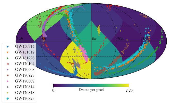
Figure 1: A sky map divided into $12$ pixels of equal area. The colour scale indicates the number of events per pixel (calculated by counting the number of posterior samples in each pixel, normalised by the total number of samples per event). About $\sim~{}2.2$ events are assigned to the highest density pixel as GW170814 and partially GW170809 are tightly localised to that pixel. Some pixels contain almost no samples; the pixel with the largest fraction of events contains $\sim~{}15$ times more samples than the pixel with the smallest fraction.

2 Analysis

The focus of this work is to represent the distribution of BBH sources on the sky. To do so, there are two readily available methods of decomposing the sky into either a finite set of pixels or spherical harmonics. In this work, for simplicity, we opt for a model that decomposes the sky into a finite set of pixels.

In this pixelated, anisotropic model we divide the sky into $N_{\mathrm{pix}}$ pixels of equal area $4\pi/N_{\mathrm{pix}}$ steradians. Each pixel $i$ has a parameter $a_{i}$, which is further referred to as a pixel weight. This pixel weight describes the stellar–mass BBH merger rate per steradian, per unit time, per unit volume within that pixel, i.e. the units of $\bm{a}$ are $\left[\bm{a}\right]=\mathrm{Gpc}^{-3}\mathrm{yr}^{-1}\mathrm{sr}^{-1}$, and both models assume homogeneous distribution of mergers within each pixel. Given that the pixel weights give the rate per steradian, we also infer the total rate $R$ ($\left[R\right]=\mathrm{Gpc}^{-3}\mathrm{yr}^{-1}$) as a sum over the whole sky,

$$R=\Delta\Omega\sum_{i}^{N_{\mathrm{pix}}}a_{i},$$ (1)

i.e. the sum of the product of pixel weights and pixel areas $\Delta\Omega$, making $R$ conditionally dependant on $\bm{a}$.

In case of the anisotropic model the number of pixels was chosen to be $N_{\mathrm{ani}}=12$, since in the subsequent analysis we work with HEALPix maps (Górski et al., 2005) and the Python package Healpy where $12$ is the minimum number of pixels available, making the analysis computationally inexpensive, while still ensuring the model has freedom to detect large-scale anisotropy. For the isotropic model we simply use $N_{\mathrm{iso}}=1$, wherein the whole sky is described by a single pixel, forcing a uniform distribution of the rate of BBH mergers.

HEALPix divides the sky into $N$ pixels with a fixed distribution. Therefore to allow for different angular distribution of pixels we introduce three Euler angles $\bm{\phi}\equiv\{\alpha,\beta,\gamma\}$ to describe the reference position and orientation of the HEALPix grid. The Euler angles $\bm{\phi}$ are used to calculate a rotation matrix to rotate the GW datasets to accommodate for different orientations of the fixed HEALpix grid.

We perform a Bayesian analysis to estimate the pixel weights $\bm{a}\equiv\{a_{i}\}$ and to perform model selection between the isotropic and anisotropic models. For a given model $I\in(\text{ISO},\text{ANISO})$, gravitational wave data sets $\{x_{j}\}$ for each of a number of detections $N_{\mathrm{obs}}$, and where $\bm{\mathrm{D}}$ indicates detection (described in Subsection 2.1), the posterior on the parameters $\bm{\theta}=\{\bm{a},\,\bm{\phi}\}$, where $\bm{a}$ are the pixel weights and $\bm{\phi}$ the Euler angles, is given by

$$\begin{split}p\left(\bm{\theta}\mid N_{\mathrm{obs}},\{x_{j}\},\bm{\mathrm{D}},I\right)&=\frac{p\left(N_{\mathrm{obs}},\{x_{j}\}\mid\bm{\theta},\bm{\mathrm{D}},I)\right)p\left(\bm{\theta}\mid\bm{\mathrm{D}},I\right)}{p\left(N_{\mathrm{obs}},\{x_{j}\}\mid\bm{\mathrm{D}},I\right)}.\end{split}$$ (2)

Having obtained the expression for the posterior (Eq. 2) we calculate the evidences for each model,

$$p\left(N_{\mathrm{obs}},\{x_{j}\}\mid\bm{\mathrm{D}},I\right)=\int p\left(N_{\mathrm{obs}},\{x_{j}\},\mid\bm{\theta},\bm{\mathrm{D}},I\right)p(\bm{\theta}\mid\bm{\mathrm{D}},I)d^{n}\bm{\theta}.$$ (3)

The ratio of evidences from the two models gives the Bayes factor, which indicates the relative support for one over the other that is imparted by a particular set of observations. For the isotropic model there is only pixel, hence one pixel weight $a_{\text{iso}}$ related to the total rate as $R=4\pi a_{\text{iso}}$. Moreover, the isotropic model is also independent of the Euler angles $\bm{\theta}$. We use the nested sampling algorithm (Skilling, 2006) in a Python package CPNest (Veitch et al., 2017) to sample the posterior and obtain the evidence for the anisotropic model. The isotropic model is evaluated analytically.

2.1 Selection function

The selection function describes the interferometer sensitivity for a given distribution of BBH mergers as a function of sky position $\Omega$ and luminosity distance $d_{\mathrm{L}}$. We consider both the O1 and O2 runs separately and define the selection function as

$$p\left(\bm{\mathrm{D}}\mid\Omega,d_{\text{L}},I\right)=\int\limits_{\rho_{\mathrm{thresh}}}^{\infty}d\rho p\left(\rho\mid\Omega,d_{\text{L}},\bm{\vartheta},I\right)p(\bm{\vartheta}|\Omega,I)p(d_{\text{L}}|I),$$ (4)

where a signal is modelled as detected if its signal-to-noise-ratio $\rho$ is measured above a predefined threshold (Abbott et al., 2019a). The probability of detection, conditional on the sky location, is computed by marginalising over the prior ranges on the distance and the remaining source parameters denoted by $\bm{\vartheta}$. The mass distribution of the primary is assumed to be a power-law $p\left(m_{1}\right)\propto m_{1}^{-2.35}$, with a minimum mass of $5\,M_{\odot}$, and the secondary to be uniformly distributed, being always less massive than the primary. A constraint is placed on the sum of the primary and secondary to be always less than $100\,M_{\odot}$. This choice of BBH mass distribution is consistent with the estimated distribution following the O1 observing run (Abbott et al., 2016a).

Since we are interested in anisotropy, we must consider the directional sensitivity of the detectors. The detectors are most sensitive to sources positioned directly above and below the detector (Anderson et al., 2001). As the Earth rotates, the antennae response function is smeared out in right-ascension, but as noted in Chen et al. (2017), there is a tendency for the detector sensitivity to vary over the course of the day due to human activity near the sites as well. This, therefore, produces a selection function which is specific to the observing conditions during a particular observing run. A full treatment of this would need to use the actual noise power spectra as a function of time throughout the observing run, but we approximate this by taking the power spectrum at the time of detections and the run-averaged power spectrum. Integrating the antenna response function over sidereal time, using a weight of one when the detector was taking science quality data, we obtain the run-averaged selection function (Vallisneri et al., 2015). We show this averaged selection for both observing runs in Fig. 4. The ratio of the maximum and minimum averaged selection function in Fig. 4 is about $1.5$ and $1.4$ for O1 and O2, respectively, indicating that in the O2 run the detectors showed marginally less preference for certain directions. This can be explained by the increased up-time of the O2 run, which reduces the overall variation in right ascension.

Fig. 2 shows the resulting selection functions (probability of detection) for O1 and O2, plotted as a function of distance for various sky positions. This shows the effect described above, with anisotropic sensitivity variations favouring the latitudes directly above the LIGO detectors, but with the response function smeared out in right ascension by the Earth’s rotation. Nonetheless, there is still some variation in right ascension, which is more pronounced for the O1 run. Comparing the two panels also shows the overall increase in detection sensitivity in the O2 run.

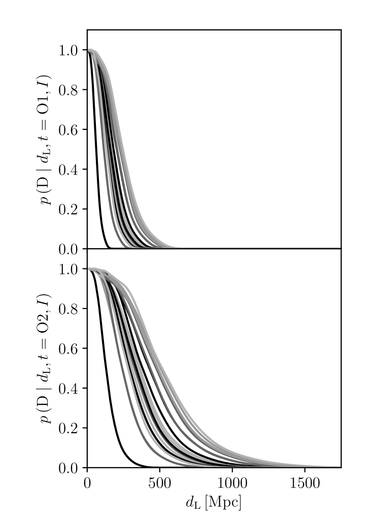
Figure 2: Comparison of survival functions for the O1 (top panel) and O2 (bottom panel) runs, where each line is the survival function sampled at a discrete sky position. The detectors are most sensitive towards directions above and below, and least sensitive to directions in the plane of the detector. There is a significant increase in sensitivity between the two runs.

Marginalising out the luminosity distance we obtain the probability of detection as a function of right ascension and declination. To calculate the probability of detection at the time of events we use the PSD estimate at the time of the BBH merger. This, along with the merger time, fully specifies the orientation of the network geometry in an Earth-fixed coordinate system which rotates in time along with the Earth. Examples of the probability of detection function for GW151226 and GW170104 are shown in Fig. 3. The figure also shows the brights spots of high probability from which a detection would be expected, given the antenna pattern, and the relative increase in sensitivity (about one order of magnitude) between the two runs. The probability of detection maps are rendered on a higher resolution map ($3,072$ pixels) compared to the $12$-pixel map of pixel weights, which describe the BBH merger rate in the anisotropic model.

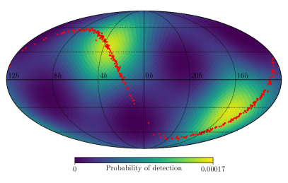
(a) $p\left(\bm{\mathrm{D}}\mid\Omega,I\right)$ at the time of GW151226.

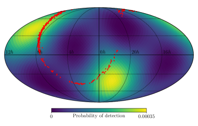
(b) $p\left(\bm{\mathrm{D}}\mid\Omega,I\right)$ at the time of GW170104.

Figure 3: Probability of detection maps at the time of GW151226 (a) from O1 run and GW170104 from O2 run (b), with the respective posterior samples scattered over. The maps were calculated with the PSD at the time of event detection and marginalising the selection function over luminosity distance. While the pattern is the same due to presence of only two LIGO detectors, the magnitude of the detection probability increases for GW170104 as the detectors were more sensitive during the O2 run.

When calculating the probability of detection we only consider the LIGO Hanford-Livingston detector network since these were the only detectors used to determine detection in the O1 and O2 runs (Abbott et al., 2019b). The Advanced Virgo detector joined at the end of the O2 run and was only used for the subsequent parameter estimation (Acernese et al., 2014), not to determine detections. Consequently, the probability of detection calculation does not include the Advanced Virgo. Nevertheless, despite Virgo’s lower sensitivity during O2 compared to the LIGO detectors, addition of its data for some of the later O2 events (such as GW170814) yielded significantly better sky localisation estimates compared to the earlier detections (Abbott et al., 2017b).

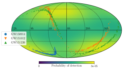
(a) Mean $\langle p\left(\bm{\mathrm{D}}\mid\Omega,I\right)\rangle$ for the O1 run

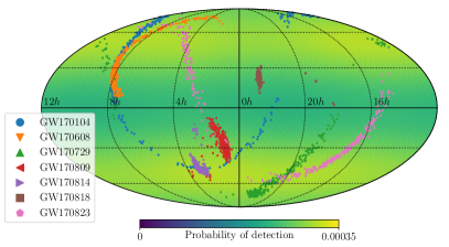
(b) Mean $\langle p\left(\bm{\mathrm{D}}\mid\Omega,I\right)\rangle$ for the O2 run

Figure 4: Mean probability of detection maps for the O1 (a) and O2 (b) runs, with posterior samples for events from O1 and O2 scattered over. The maps were calculated with the average PSD for each run, marginalising the selection function over distance and time averaging the $p\left(\bm{\mathrm{D}}\mid\Omega,t,I\right)$, where $t$ is the GPS time, over the times the detectors were operational.

2.2 Prior

In the isotropic model, the only free parameter of the model is $R$, the overall rate of BBH mergers (Eq. 1). We choose a Jeffreys prior,

$$p\left(R\mid\mathrm{ISO}\right)\propto R^{-1/2},$$ (5)

which allows a direct comparison with rate estimates published by the LIGO-Virgo Collaboration using sophisticated measurements of sensitive time-volume and models of the source population (Abbott et al., 2019c).

In the anisotropic model with $N_{\mathrm{pix}}$ equal-area pixels, we have parameters $a_{1},\ldots,a_{N_{\mathrm{pix}}}$. Since we wish to compare it to the isotropic model, we specify the prior on the overall rate $R$ to have the same Jeffreys form as Eq. 5, so

$$p\left(R\mid\mathrm{ANISO}\right)\propto R^{-1/2}\propto\int p\left(R\mid\bm{a}\right)p\left(\bm{a}\mid\mathrm{ANISO}\right)d^{N_{\mathrm{pix}}}\bm{a}.$$ (6)

Since we do not favour any particular pixel a-priori, the prior should be symmetric under $a_{i}\leftrightarrow a_{j}$. The following prior fulfils this criteria, while being uniform on the $N-1$-simplex of possible $\bm{a}$s for a particular $R$,

$$p(\vec{a}|\mathrm{ANISO})\propto R^{-(2N_{\mathrm{pix}}-1)/2}=\left(\frac{4\pi}{N_{\mathrm{pix}}}\sum_{i}^{N_{\mathrm{pix}}}a_{i}\right)^{-(2N_{\mathrm{pix}}-1)/2}.$$ (7)

Pixel weight $a_{i}$	$\left[0,\,25\right]\,\mathrm{Gpc}^{-3}\mathrm{yr}^{-1}\mathrm{sr}^{-1}$
Total astrophysical rate $R$	$\left[10^{-5},\,750\right]\mathrm{Gpc}^{-3}\mathrm{yr}^{-1}$
First Euler angle about the $z$-axis $\alpha$	$\left[0,2\pi\right]$
Second Euler angle about the $y$-axis $\cos\beta$	$\left[0.75,1\right]$
Third Euler angle about the $z$-axis $\gamma$	$\left[0,2\pi\right]$

Table 1: Prior ranges on the inferred parameters $\bm{\theta}$ and the total rate $R$.

Boundaries found in Table 1 are applied to the inferred parameters. Note that the boundary on the total rate $R$ is well outside of the range found by the O1 and O2 run (Abbott et al., 2019c). The Euler angles rotate the angular distribution of pixels, however without restricting the range of rotations the posterior would become strongly degenerate as multiple combinations of the Euler angles would correspond to the identical orientation of the HEALpix grid. Our intent in setting the boundaries for the Euler angles is twofold. First, we choose a uniform rotation prior over the ranges as shown in Table 1. Second, to avoid degeneracy of the likelihood we enforce a condition wherein no pixel centre can be rotated beyond its original boundary. An example of this degeneracy is rotating the pixel grid about the $z$-axis by an angle that corresponds to the angular separation of two nearby pixel centres that lie in in the $x-y$ plane. The range of $\cos\beta$ was restricted (Table 1) as values outside this range would violate the aforementioned second condition.

2.3 Likelihood

In our specific problem, the likelihood $p(N_{\mathrm{obs}},\{x_{j}\}\mid\bm{\theta},I)$ depends on the data for each detected event (yielding estimates of their sky position, distance, masses and detection time) and the selection function. The likelihood can be split into the so-called number and event likelihood respectively,

$$p\left(N_{\mathrm{obs}},\{x_{j}\}\mid\bm{\theta},\bm{\mathrm{D}},I\right)=P\left(N_{\mathrm{obs}}\mid\bm{\theta},\bm{\mathrm{D}},I\right)p\left(\{x_{j}\}\mid\bm{\theta},\bm{\mathrm{D}},I\right),$$ (8)

where $\bm{\mathrm{D}}$ indicates detection and the use of the interferometers’ PSDs (Mandel et al., 2019).

If we divide the observation time into $n$ segments, and assume the probability of detection to be constant over the segment duration, then we can write the probability of detecting $N_{\mathrm{obs}}$ events as a Poisson binomial distribution, that is

$$\begin{split}P\left(N_{\mathrm{obs}}\mid\bm{\theta},\bm{D},I\right)&=\binom{n}{N_{\mathrm{obs}}}\prod_{j=1}^{N_{\mathrm{obs}}}p\left(N\geq 1\mid\bm{\theta},\bm{\mathrm{D}}_{j},I\right)\\ &\times\prod_{k=1}^{n-N_{\mathrm{obs}}}P\left(N=0\mid\bm{\theta},\bm{\mathrm{D}}_{k},I\right),\end{split}$$ (9)

so that $\bm{\mathrm{D}}_{j,k}$ is the probability of detection evaluated in the $j$-th segment. We define success as drawing $1$ or more events within a segment and a failure as drawing no events,

$$p\left(N=0\mid\bm{\theta},\bm{\mathrm{D}}_{k},I\right)=\exp\left[-\hat{N}_{k}\right],$$ (10)

where $\hat{N}_{k}$ is the expected number of detections from the $k$-th segment and $p\left(N\geq 1\mid\bm{\theta},\bm{\mathrm{D}}_{k},I\right)=1-p\left(N=0\mid\bm{\theta},\bm{\mathrm{D}}_{k},I\right)$. In the limit of large $n$ (equivalently $\hat{N}_{j}\ll 1$), we may approximate Eq. (9) as

$$P\left(N_{\mathrm{obs}}\mid\bm{\theta},\bm{D},I\right)\propto\left(\prod_{j=1}^{N_{\mathrm{obs}}}\hat{N}_{j}\right)\exp\left[-\sum_{k=1}^{n}\hat{N}_{k}\right].$$ (11)

The number of expected detections in the $j$-th time segment of duration $\mathrm{d}t$ is the convolution of the differential rate and the probability of detection:

$$\hat{N}_{j}=\mathrm{d}tV_{\mathrm{L}}\int\derivative{R}{\Omega}p\left(\bm{\mathrm{D}}_{j}\mid\Omega,I\right)\mathrm{d}\Omega.$$ (12)

First, because in the anisotropic model we allow the astrophysical merger rate to vary with sky position, we cannot fully separate it when considering the number of detections from a given time segment in Eq. (12). Second, for both models we assume homogeneity, therefore $V_{\mathrm{L}}$, the luminosity volume, can be taken outside the integral in Eq. (12) as long as $V_{\mathrm{L}}$ matches the volume over which we marginalised out the probability of detection function. Because the detection probability vanishes at sufficiently high distances, our result will be independent of the choice of $V_{\mathrm{L}}$, provided we consider a volume much larger than the observable one.

For this analysis we have assumed a simple distance prior, independent of sky location, $p\left(d_{\mathrm{L}}\right)\propto d_{\text{L}}^{2}$, which is consistent with a static, Euclidean universe. Similarly, we have also assumed an underlying astrophysical rate that is constant with distance (and therefore with redshift). As our primary aim is to test anisotropy, and not homogeneity, coupled with the fact that the detections are positioned in the local Universe, we expect that the impact of these assumptions (which are shared by both models) to be a second order effect. The probability density function of a sky position $p\left(\Omega\mid\bm{\theta}\right)$ is taken to be uniform within each pixel, proportional to its weight $a_{i}$ and time-independent.

An underlying assumption of our models is that the sky can be pixelated and that the astrophysical rate and probability of detection are uniform over each pixel (we render the probability of detection on a higher-resolution basis). Thus, the differential rate $\mathrm{d}R/\mathrm{d}\Omega$ is equal to the pixel’s weight, and Eq. (12) simplifies to

$$\hat{N}_{j}=V_{\mathrm{L}}\frac{T}{n}\sum_{k=1}^{N_{\mathrm{pix}}}a_{k}\,p\left(\bm{\mathrm{D}}_{j}\mid\Omega_{k},I\right)\Delta\Omega,$$ (13)

where $a_{k}$, $\Omega_{k}$, and $\Delta\Omega$ indicate the $k$-th pixel’s weight, sky location, and angular area, respectively. We also set the segment duration to be $\mathrm{d}t=T/n$, with $T$ being the observing run duration and $n$ the number of segments.

In Eq. (11) we require the sum of the expected number of detections over all segments: $\hat{N}=\sum_{j=1}^{n}\hat{N}_{j}$. Since we assume the pixel weights to be time-independent, the sum over individual segments then simplifies to

$$\hat{N}=V_{\mathrm{L}}T\sum_{k=1}^{N_{\mathrm{pix}}}a_{k}\,\langle p\left(\bm{\mathrm{D}}\mid\Omega_{k},I\right)\rangle\Delta\Omega,$$ (14)

where $\langle p\left(\bm{\mathrm{D}}\mid\Omega_{k},I\right)\rangle=1/n\sum_{j=1}^{n}p\left(\bm{\mathrm{D}}_{j}\mid\Omega_{k},I\right)$ is the probability of detection as a function of sky position averaged over the times when the interferometers were operating. The expected number of events is evaluated separately for O1 and O2, as the selection function and observation times differ for each run.

The event likelihood in Eq. (8) can be split into a product over all events, assuming they are independent of each other,

$$p\left(\{x_{j}\}\mid\bm{\theta},\bm{\mathrm{D}}_{j},I\right)=\prod_{j=1}^{N_{\mathrm{obs}}}p\left(x_{j}\mid\bm{\theta},\bm{\mathrm{D}}_{j},I\right).$$

This can be further expanded using the Bayes’s theorem, noting that the likelihood $p\left(\bm{\mathrm{D}}_{j}\mid x_{j},\bm{\theta},I\right)=1$ for detections:

$$\begin{split}p\left(x_{j}\mid\bm{\theta},\bm{\mathrm{D}}_{j},I\right)&=\frac{p\left(x_{j}\mid\bm{\theta},I\right)}{p\left(\bm{\mathrm{D}}_{j}\mid\bm{\theta},I\right)}\\ &=\frac{\iint\mathrm{d}\Omega\mathrm{d}d_{\mathrm{L}}p\left(x_{j}\mid\Omega,d_{\mathrm{L}},I\right)p\left(\Omega,d_{\mathrm{L}}\mid\bm{\theta},I\right)}{\int\mathrm{d}\Omega p\left(\bm{\mathrm{D}}_{j}\mid\Omega,I\right)p\left(\Omega,\mid\bm{\theta},I\right)}.\end{split}$$ (15)

We expand both the prior (numerator) and the evidence (denominator) on the first line of Eq. (15) using the marginalisation rule. Furthermore, in Eq. (15) the prior can be Monte Carlo approximated over the GWOSC posterior samples (indexed by $i$). The GWOSC posterior samples assume a uniform prior over component masses, whereas in our probability of detection calculation we assumed a power-law distribution. To correct for this, we add our component mass prior to the GWOSC samples. The evidence in Eq. (15) does not depend on the GWOSC samples, only on the run-averaged probability of detection and so can be marginalised over distance. With this in mind the final approximate expression for Eq. (15) becomes

$$p\left(x_{j}\mid\bm{\theta},\bm{\mathrm{D}}_{j},I\right)\approx\frac{\sum_{i=1}^{N_{j}}p\left(\Omega_{j}^{i}d_{\mathrm{L},j}^{i}\mid\bm{\theta},I\right)p\left(m_{1,j}^{i},m_{2,j}^{i}\mid\alpha\right)/N_{j}}{\sum_{k=1}^{N_{\mathrm{pix}}}\Delta\Omega p\left(\bm{\mathrm{D}}_{j}\mid\Omega_{k},I\right)p\left(\Omega_{k}\mid\bm{\theta},I\right)},$$ (16)

where $p\left(m_{1},m_{2}\mid\alpha\right)$ is our component mass prior and $N_{j}$ is the number of posterior samples for the $j$-th detection. The selection function $p(\bm{\mathrm{D}}_{j}\mid\Omega,I)$ is evaluated at the time of detection of the $j$-th event with the event’s PSD. Furthermore, in the final expression for the likelihood, the denominator of Eq. (16) cancels with $\hat{N}_{j}$ (Eq. 12) as $p\left(\Omega_{k}\mid\bm{\theta}\right)\propto a_{k}$.

3 Results

The isotropic model is parametrised by a single pixel covering the entire sky, making it invariant under the angular distribution of pixels and independent of the Euler angles. On the other hand, the anisotropic model spans a $15$-dimensional parameter space. Each posterior sample in the anisotropic model contains a set of $12$ pixel weights and its associated Euler angles describing the orientation of the HEALPix grid. It follows then that in each sample the pixels correspond to different locations on the sky, which is accounted for before averaging the pixel weights. In Fig. 5 we show the maximum likelihood sample for the anisotropic model. To average the pixel weights, the original $12$ pixels are split into a set of $49,152$ pixels which map the samples onto a finer basis, while preserving their respective values. This larger set is rotated and then averaged out as this corresponds to returning to the original coordinate system, resulting in a smoothing of the original $12$-dimensional pixel basis and rendering the mean pixel weights on a higher resolution map.

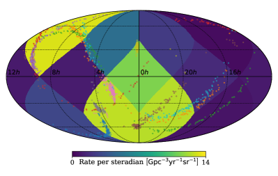
Figure 5: Example of a posterior sample for the anisotropic model, corresponding to the maximum likelihood probability. The GW event samples are rotated relative to the original coordinate system (Fig. 1).

The averaged pixel map of posterior samples for the anisotropic model is shown in Fig. 8. Two parts of the sky have above average values of rate density, corresponding to the areas with the highest density of samples (Fig. 1). However, the ratio of the maximum to the minimum rate densities is $\sim{3}$, while the ratio of the maximum to the minimum number of GW event posterior samples per pixel is $\sim{15}$ (Fig. 1), illustrating how the selection functions differs between our posterior and a simple samples count.

Anisotropic model total rate ${R}_{\mathrm{ani}}$	$60.5^{+33.4}_{-25.4}\,\mathrm{Gpc}^{-3}\mathrm{yr}^{-1}$
Isotropic model total rate ${R}_{\mathrm{iso}}$	$58.9^{+42.4}_{-23.0}\,\mathrm{Gpc}^{-3}\mathrm{yr}^{-1}$
LVC total rate $R_{\mathrm{LVC}}$	$53.2^{+58.5}_{-28.8}\,\mathrm{Gpc}^{-3}\mathrm{yr}^{-1}$
Bayes factor $\mathcal{Z}_{\text{ISO}}/\mathcal{Z}_{\text{ANISO}}$	$1.3:1$

Table 2: Comparison of the total rate of our models with the LVC result and the Bayes factor ratio of the isotropic and anisotropic model.

Furthermore, we obtain estimates of the total rate $R$ (defined in Eq. 1), as in our analysis the merger rate is proportional to the sum of the pixel weights. In Fig. 6 we show a histogram of the total rate for the two models and quote our results with $90\%$ credibility intervals in Table 2.

The confidence intervals we obtain are tighter than the LVC estimate of the total rate (Abbott et al., 2019c). This distinction can be attributed to a number of differing assumptions between the LVC analysis and our own. These include, but are not limited to the facts that our analysis makes different prior assumptions about the black hole mass distribution, and that we do not marginalise over uncertainty in the mass power law index and our model assumes a maximum total mass. In addition, we have not used a realistic cosmological model for our redshift distribution, we have considered only the inspiral component of the signal waveform as opposed to the full inspiral, merger, and ringdown, and our selection function is computed analytically and not empirically from simulated signal injections into real non-Gaussian detector noise.

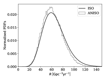
Figure 6: Posterior probability distributions on the rate $R$ of BBH mergers, assuming the isotropic and anisotropic models. The isotropic model is consistent the LVC estimate of the total rate $53.2^{+58.5}_{-28.8}\,\mathrm{Gpc}^{-3}\mathrm{yr}^{-1}$ of BBH mergers.

To determine whether the BBH mergers are distributed isotropically on the sky, we calculate a Bayes factor between the two hypotheses (defined in Eq. 3). We arrive at a Bayes factor $\mathcal{Z}_{\mathrm{ISO}}/\mathcal{Z}_{\mathrm{ANI}}$ of $1.3:1$, indicating that the $10$ events from O1 and O2 runs show no statistically significant preference for either model.

Lastly, we test our model by replacing all the observed events from O1 and O2 with $n=1,2,\ldots,10$ copies of GW170814 and record the Bayes factors $\mathcal{Z}_{\mathrm{ISO}}/\mathcal{Z}_{\mathrm{ANISO}}$ as a function of $n$. This is shown in Fig. 7. We observe an exponential dependence on $n$, with isotropy being preferred for low values of $n$ but gradually showing strong support for anisotropy as $n$ increases.

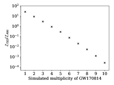
Figure 7: Bayes factor $\mathcal{Z}_{\mathrm{ISO}}/\mathcal{Z}_{\mathrm{ANISO}}$ when all events from O1 and O2 runs are replaced with $n=1,2,\ldots,10$ copies of GW170814. Initially, for low values of $n$, the data prefers the isotropic model but as $n$ increases and more events are added into the same location the confidence in the anisotropic model exponentially grows.

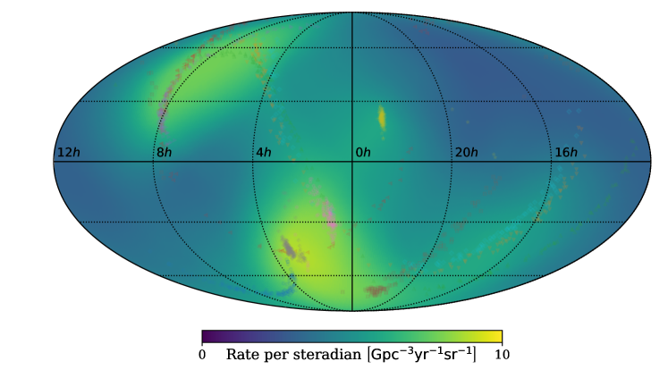
Figure 8: A mean map of pixel weights averaged over the different rotations of the posterior distributions such as Fig. 5. The individual samples were rendered on a smoother basis of $49,152$ pixels (the weights are defined per steradian, thus independent of the pixel size), rotated to a default frame of reference and averaged. The ratio of the maximum to the minimum rate density of the map is $\sim~{}3$.

4 Conclusion

We perform a Bayesian model selection, comparing an isotropic model to a particular pixelated anisotropic model of the BBH astrophysical merger rate. We demonstrate that the $10$ detected BBH events from O1 and O2 runs show comparable support for both models. This result was expected, the underlying distribution of BBH mergers is thought to be isotropic, but with only $10$ events forming our dataset a strong statement about isotropy should not be expected.

The anisotropic model is described with $15$ parameters which give a very large parameter space for the model, most of which is incompatible with the data. Since we made a decision to use a pixel basis, and the minimum number of pixels a HEALpix map supports is $12$, it was not possible to easily switch to a lower or higher dimensional basis. Thus, one of the future extensions of this project would be to to perform this analysis in a spherical harmonics basis. A spherical harmonic basis would allow for a lower dimensional parameter space, for example, the simplest anisotropic spherical harmonics model would have $4$ weight parameters (polynomial degree $l_{\mathrm{max}}=1$). Such spherical harmonic approaches could be readily used to model different anisotropy models, providing us with an alternative representation with which to compare the benchmark isotropic model. This approach is taken by Payne et al. (2020), which also finds that the GWTC-1 data-set weakly favours the isotropic model, although their analysis differs from ours in other respects.

In this analysis the prior probability density function (PDF) on luminosity distance is consistent with that of a simple, static Euclidean universe. As the interferometers are being upgraded in terms of sensitivity it would be reasonable to include a cosmological model of an expanding universe since some events are already at significant redshifts. However, we do not expect this to change the result dramatically, rather it should result in scaling the selection function and providing us with better tools that could be used in further applications.

Finally, and potentially most importantly, at the time of writing, only ten events (from O1 and O2) have been published by the LIGO-Virgo Collaboration. The recently finished O3 run lived up to expectations and provided $\sim~{}60$ additional candidates and the O3 events are generally better localised due to sensitivity improvements at the Virgo site (LIGO-Virgo Collaboration, 2020). Such additional data will only serve to strengthen the analysis presented here and we are eager to use these events to compare our BBH distribution models. In the future we predict that this work can be used to significantly strengthen our belief in the isotropic model over an anisotropic model as the number of detections increases. Alternatively, the analysis can be interpreted as an important probe for finding anisotropies, should they exist. In the limit of a large number of detections, if BBH sources trace the large scale structure of the Universe we might expect that a general anisotropic model might be favoured over isotropy. This scenario would allow us to meaningfully compare our results to the distribution of visible matter in the Universe.

Data Availability

The data underlying this article will be shared on reasonable request to the corresponding author.

References

- Abbott et al. (2016a) Abbott B. P., et al., 2016a, Phys. Rev. X, 6, 041015
- Abbott et al. (2016b) Abbott B. P., et al., 2016b, Phys. Rev. Lett., 116, 061102
- Abbott et al. (2016c) Abbott B. P., et al., 2016c, Astrophys. J. Lett., 833, L1
- Abbott et al. (2017a) Abbott B. P., et al., 2017a, Phys. Rev. Lett., 118, 221101
- Abbott et al. (2017b) Abbott B. P., et al., 2017b, Phys. Rev. Lett., 119, 141101
- Abbott et al. (2017c) Abbott B. P., et al., 2017c, Ap. J. Lett., 851, L35
- Abbott et al. (2018) Abbott B. P., et al., 2018, Living Rev. Rel., 21, 3
- Abbott et al. (2019a) Abbott B. P., et al., 2019a, preprint (arXiv:1908.06060)
- Abbott et al. (2019b) Abbott B. P., et al., 2019b, Phys. Rev., X9, 031040
- Abbott et al. (2019c) Abbott B. P., et al., 2019c, Astrophys. J., 882, L24
- Acernese et al. (2014) Acernese F., et al., 2014, Classical and Quantum Gravity, 32, 024001
- Anderson et al. (2001) Anderson W. G., Brady P. R., Creighton J. D. E., Flanagan E. E., 2001, Phys. Rev. D, 63, 042003
- Chen et al. (2017) Chen H.-Y., Essick R., Vitale S., Holz D. E., Katsavounidis E., 2017, Astrophys. J., 835, 31
- Daniel Sigg (2016a) Daniel Sigg 2016a, H1 Calibrated Sensitivity Spectra Oct 24 2015 (Representative for O1), https://dcc.ligo.org/LIGO-G1600150/public
- Daniel Sigg (2016b) Daniel Sigg 2016b, L1 Calibrated Sensitivity Spectra Oct 24 2015 (Representative for O1), https://dcc.ligo.org/LIGO-G1600151/public
- Dominik et al. (2015) Dominik M., Berti E., O’Shaughnessy R., Mandel I., et al., 2015, ApJ, 806, 263
- Górski et al. (2005) Górski K. M., Hivon E., Banday A. J., Wandelt B. D., Hansen F. K., Reinecke M., Bartelmann M., 2005, ApJ, 622, 759
- Harry (2010) Harry G. M., 2010, Class. Quant. Grav., 27, 084006
- Horvath et al. (2013) Horvath I., Hakkila J., Bagoly Z., 2013, arXiv e-prints, p. arXiv:1311.1104
- LIGO Scientific Collaboration (2015) LIGO Scientific Collaboration 2015, Class. Quantum Grav., 32, 074001
- LIGO-Virgo Collaboration (2018) LIGO-Virgo Collaboration 2018, GWTC-1, https://dcc.ligo.org/LIGO-P1800374/public
- LIGO-Virgo Collaboration (2019) LIGO-Virgo Collaboration 2019, Power Spectral Densities (PSD) release for GWTC-1, https://dcc.ligo.org/LIGO-P1900011/public
- LIGO-Virgo Collaboration (2020) LIGO-Virgo Collaboration 2020, Gravitational-Wave Candidate Event Database, https://gracedb.ligo.org/superevents/public/O3/
- Mandel et al. (2019) Mandel I., Farr W. M., Gair J. R., 2019, Mon. Not. Roy. Astron. Soc., 486, 1086
- Ng et al. (2018) Ng K. K. Y., Vitale S., Zimmerman A., Chatziioannou K., Gerosa D., Haster C.-J., 2018, Phys. Rev., D98, 083007
- O’Shaughnessy et al. (2010) O’Shaughnessy R., Vaishnav B., Healy J., Shoemaker D., 2010, Phys. Rev. D, 82, 104006
- Payne et al. (2020) Payne E., Banagiri S., Lasky P., Thrane E., 2020, arXiv e-prints, p. arXiv:2006.11957
- Saadeh et al. (2016) Saadeh D., Feeney S. M., Pontzen A., Peiris H. V., McEwen J. D., 2016, Phys. Rev. Lett., 117, 131302
- Singer & Price (2016) Singer L. P., Price L., 2016, Phys. Rev. D, 93, 024013
- Skilling (2006) Skilling J., 2006, Bayesian Anal., 1, 833
- Vallisneri et al. (2015) Vallisneri M., Kanner J., Williams R., Weinstein A., Stephens B., 2015, in Journal of Physics Conference Series. p. 012021 (arXiv:1410.4839), doi:10.1088/1742-6596/610/1/012021, https://www.gw-openscience.org/about/
- Veitch et al. (2015) Veitch J., et al., 2015, Phys. Rev. D, 91, 042003
- Veitch et al. (2017) Veitch J., Del Pozzo W., Cody Pitkin M., ed1d1a8d 2017, http://www.github.com/johnveitch/cpnest, doi:10.5281/zenodo.835874, https://doi.org/10.5281/zenodo.835874
- Virgo Collaboration (2014) Virgo Collaboration 2014, Class. Quantum Grav., 32, 024001