A Theory of Computational Resolution Limit for Line Spectral Estimation

Abstract

Line spectral estimation is a classical signal processing problem that aims to estimate the line spectra from their signal which is contaminated by deterministic or random noise. Despite a large body of research on this subject, the theoretical understanding of this problem is still elusive. In this paper, we introduce and quantitatively characterize the two resolution limits for the line spectral estimation problem under deterministic noise: one is the minimum separation distance between the line spectra that is required for exact detection of their number, and the other is the minimum separation distance between the line spectra that is required for a stable recovery of their supports. The quantitative results imply a phase transition phenomenon in each of the two recovery problems, and also the subtle difference between the two. We further propose a sweeping singular-value-thresholding algorithm for the number detection problem and conduct numerical experiments. The numerical results confirm the phase transition phenomenon in the number detection problem.

Keywords: Line spectral estimation, resolution limit, phase transition.

1 Introduction

This paper is concerned with recovering the number and supports of a collection of line spectra from their contaminated signal, which is usually termed the line spectral estimation (LSE) problem. It is at the core of diverse research fields such as wireless communication, radar, sonar, seismology and astronomy, and has received significant attention over the years. While the LSE problem was usually cast as a statistical parameter estimation problem with random noise in the measurement, we are interested in the case of deterministic noise. To be more specific, we consider the following mathematical model. Let $\mu=\sum_{j=1}^{n}a_{j}\delta_{y_{j}}$ be a discrete measure, where $y_{j}\in\mathbb{R},j=1,\cdots,n$, represent the supports of the line spectra and $a_{j}\in\mathbb{C},j=1,\cdots,n$ their amplitudes. We assume that $|y_{j}|\leq d$ for all $j$. We denote

$$m_{\min}=\min_{j=1,\cdots,n}|a_{j}|,\quad d_{\min}=\min_{p\neq j}|y_{p}-y_{j}|.$$

We sample the Fourier transform of $\mu$ at $M$ equispaced points:

$$\mathbf{Y}(\omega_{q})=\mathcal{F}\mu(\omega_{q})+\mathbf{W}(\omega_{q})=\sum_{j=1}^{n}a_{j}e^{iy_{j}\omega_{q}}+\mathbf{W}(\omega_{q}),\quad 1\leq q\leq M,$$ (1.1)

where $\omega_{1}=-\Omega,\omega_{2}=-\Omega+h,\cdots,\omega_{M}=\Omega$. Here $h=\frac{2\Omega}{M-1}$ is the sampling spacing and $\mathbf{W}(\omega_{q})$’s are the noise. We assume that $|\mathbf{W}(\omega_{q})|<\sigma$ with $\sigma$ being the noise level. Throughout, we assume that $M>2n$ and that $h\leq\frac{\pi}{d}$. The latter assumption excludes the non-uniqueness of the line spectra due to shifts by multiples of $\frac{2\pi}{h}$. Denote

$$\mathbf{Y}=(\mathbf{Y}(\omega_{1}),\cdots,\mathbf{Y}(\omega_{M}))^{T},\quad[\mu]=(\mathcal{F}\mu(\omega_{1}),\cdots,\mathcal{F}\mu(\omega_{M}))^{T}\quad\text{and}\quad\mathbf{W}=(\mathbf{W}(\omega_{1}),\cdots,\mathbf{W}(\omega_{M}))^{T}.$$

Then the noisy measurement can be written in the following form

$$\mathbf{Y}=[\mu]+\mathbf{W}.$$

The LSE problem we are interested in is to recover the discrete measure $\mu$ from the above noisy measurement $\mathbf{Y}$. We note that the LSE problem is closely related to the deconvolution problem in imaging where the measurement is the convolution of point sources and a band-limited point spread function $f$. More precisely, in the presence of additive noise $\epsilon(t)$, the measurement is

$$y(t)=\mu*f(t)+\epsilon(t)=\sum_{j=1}^{n}a_{j}f(t-y_{j})+\epsilon(t).$$ (1.2)

By taking the Fourier transform on both sides, we obtain

$$\mathcal{F}y(\omega)=\mathcal{F}f(\omega)\cdot\mathcal{F}\mu(\omega)+\mathcal{F}\epsilon(\omega)=\mathcal{F}f(\omega)(\sum_{j=1}^{n}a_{j}e^{iy_{j}\omega})+\mathcal{F}\epsilon(\omega),$$ (1.3)

which is reduced to the LSE problem.

1.1 Literature review

It is well-known, since Rayleigh’s work [41], that two sources (or line spectra as are called in this paper) can be resolved if they are separated more than the Rayleigh limit (or Rayleigh length in some literature) $\frac{\pi}{\Omega}$. Although it is an empirical limit, the Rayleigh limit plays an important role in many source or line spectra resolving algorithms. For example, it is proved that TV minimization can exactly resolve off-the-grid sources from their noiseless low-frequency measurement if they are separated more than several Rayleigh limits [8]. See also [7, 18, 17] for the related researches in the resolving ability of TV minimization. Other sparsity promoting optimization based algorithms such as the BLASSO [4, 16, 39] and the atomic norm minimization [52, 51, 10] can also provably recover the off-the-grid sources under a minimum separation of several Rayleigh limits or certain non-degeneracy condition. This minimum separation requirement is necessary for general source recovery [16, 50, 28, 39], but can be relaxed for positive sources [14, 37, 36].

As the source separation distance decreases and falls below the Rayleigh limit, it becomes increasingly difficult to resolve them from the noisy measurement. In such sub-Rayleigh regime, a variety of parametric methods, including Prony’s method [40], MUSIC [44, 49], ESPRIT [43] and Matrix Pencil method [25, 26] are shown to have favourable performance. In general, parametric methods require a priori information of the model order (or the number of line spectra) and their performances depend on it sensitively [21]. We note that ESPRIT and MUSIC algorithms are analyzed recently in [30, 29]. We also refer to [6] for the numerical performance of the Matrix Pencil method.

Despite much progress in the development of algorithms, the theoretical understanding of the resolution limit is still elusive. A particular puzzle is the gap between the physical (classical) resolution limit and the limit from a data processing point of view. Precisely, the empirical Rayleigh limit is based on presumed resolving capabilities of the human visual system and is not useful for data elaborately processed, see for instance [38, 13]. In the last century, this resolution limit puzzle had drawn much attention and was investigated extensively from the perspective of statistical estimation and hypothesis testing, see for instance [23, 24, 34, 33, 12]. Most of the studies focus on the two-point resolution limit which is defined to be the minimum detectable distance between two point sources at a given signal-to-noise ratio (SNR). Especially, in [46, 47, 48], by unifying and generalizing much of the literature on the topic which spanned the course of roughly four decades, the authors derived explicit formula for the minimum SNR that is required to discriminate two point sources separated by a distance smaller than the Rayleigh limit. It is shown that the required SNR is inversely proportional to a certain power of the source separation distance and the power is different from case to case.

On the other hand, Donoho first addressed the resolution limit from the optimal recovery point of view [15]. He considered measures supported on the lattice $\{k\Delta\}_{k=-\infty}^{+\infty}$ and regularized by the so-called “Rayleigh index”. He showed that the minimax error for the amplitude recovery with noise level $\sigma$ scales like $SRF^{\alpha}\sigma$, where $SRF=\frac{1}{\Omega\Delta}$ is the super-resolution factor, and $\alpha$ is a parameter depends on the Rayleigh index. This result highlights the importance of sparsity and SNR in the ill-posedness of this inverse problem. Further discussed in [11], the authors considered the case of $n$-sparse signals supported on a grid and showed that the scaling of the noise level for the minimax error should be $SRF^{2n-1}$. See also similar results for the multi-clumps case in [29, 5]. However, these works mostly deal with the grid setting and do not address the recovery of source supports.

In [35], under the off-the-grid setting, using novel extremal functions, the author established a sharp phase transition for the amplitude and support recovery in the relation between cutoff frequency ($\Omega$) and separation distance ($\Delta$). Recently in [3] the authors derived the required SNR for a stable recovery of supports in the LSE problem. They further derived sharp minimax errors for the support and the amplitude recovery in [6]. More precisely, they showed that for $\sigma\lessapprox(SRF)^{-2p+1}$, where $p$ is the number of nodes (or the line spectra as are called in this paper) which form a cluster of certain type, the minimax error rate for reconstruction of the clustered nodes is of the order $(SRF)^{2p-2}\frac{\sigma}{\Omega}$, while for recovering the corresponding amplitudes the rate is of the order $(SRF)^{2p-1}\sigma$. Moreover, the corresponding minimax rates for the recovery of the non-clustered nodes and amplitudes are $\frac{\sigma}{\Omega}$ and $\sigma$ respectively. In an earlier work [32] by the authors of the paper, the computational resolution limit was proposed for the deconvolution problem (1.2). By working directly with the measurement in (1.2) other than the Fourier data in (1.3), and employing a multipole expansion method, they showed that the resolution limit for number detection is bounded above by $\frac{C(d)}{\Omega}\left(\frac{\sigma}{\sigma_{\min}(s)m_{\min}}\right)^{\frac{1}{2n-2}}$, where $C(d)$ is a constant depending on the interval with size $d$ where all the $n$ sources are located and $\sigma_{\min}(s)$ is a positive number characterizing the correlation of the multipoles used in the reconstruction. Similar result on the resolution limit for the support recovery was obtained as well. This paper deals with the LSE problem. It can be viewed as an investigation for the deconvolution problem with Fourier measurement. The results obtained herein improves the bounds in [32] by getting rid of the factor $\sigma_{\min}(s)$.

1.2 Main contribution

In this paper, we investigate the LSE problem for a cluster of closely spaced line spectra in the off-the-grid setting with deterministic noise. The main contribution is a quantitative characterization of the resolution limit to the spectral number detection problem. Accurate detection of the spectral number (or the model order in some literature) is an important step in the LSE problem and many parametric estimation methods require the spectral number as a priori information. But there is few theoretical result which addresses the issue when this number is greater than two. The results we derived in the paper seem to be the first in this direction to our knowledge. To resolve this issue, we introduce the computational resolution limit $\mathcal{D}_{num}$ for the detection of $n$ spectra (see Definition 2.2) where $n$ can be an arbitrary integer greater than or equal to two, and derive the following sharp bounds:

$$\frac{0.81e^{-\frac{3}{2}}}{\Omega}\Big{(}\frac{\sigma}{m_{\min}}\Big{)}^{\frac{1}{2n-2}}<\mathcal{D}_{num}\leq\frac{4.4\pi e}{\Omega}\Big{(}\frac{\sigma}{m_{\min}}\Big{)}^{\frac{1}{2n-2}},$$ (1.4)

where $\frac{\sigma}{m_{\min}}$ is viewed as the inverse of the SNR. It follows that with deterministic noise, exact detection of the spectral number is possible when the minimum separation distance of line spectra $d_{\min}$ is greater than $\frac{4.4\pi e}{\Omega}\Big{(}\frac{\sigma}{m_{\min}}\Big{)}^{\frac{1}{2n-2}}$, and impossible without additional a priori information when $d_{\min}$ is less than $\frac{0.81e^{-\frac{3}{2}}}{\Omega}\Big{(}\frac{\sigma}{m_{\min}}\Big{)}^{\frac{1}{2n-2}}$. The quantitative characterization of the resolution limit $\mathcal{D}_{num}$ implies a phase transition phenomenon in the number detection problem. We further propose a sweeping singular-value-thresholding algorithm for the number detection and conduct numerical experiments which confirm the prediction (see Section 5). The main technique used to derive the bounds for the resolution limit is the approximation theory in Vandermonde space (see Section 3). The approximation theory was first introduced in the authors’ paper [32] for real Vandermonde vectors. We generalize the theory to the case of complex vectors in this paper.

Following the same line of argument for the number detection problem, we also consider the support recovery problem in LSE. We introduced the computational resolution limit $\mathcal{D}_{supp}$ for the support recovery (see Definition 2.4) and derive the following bounds:

$$\frac{0.49e^{-\frac{3}{2}}}{\Omega}\Big{(}\frac{\sigma}{m_{\min}}\Big{)}^{\frac{1}{2n-1}}<\mathcal{D}_{supp}\leq\frac{5.88\pi e}{\Omega}\Big{(}\frac{\sigma}{m_{\min}}\Big{)}^{\frac{1}{2n-1}}.$$ (1.5)

As a consequence, the resolution limit $\mathcal{D}_{supp}$ is of the order $O(\Big{(}\frac{\sigma}{m_{\min}}\Big{)}^{\frac{1}{2n-1}})$. We also show that when the minimum separation distance exceeds the upper bound of $\mathcal{D}_{supp}$, the deviation of recovered supports to the ground truth scales as $SRF^{2n-2}\frac{\sigma}{\Omega m_{\min}}$. Such results were also reported in the closely related work [6] under a more general setting where some of the line spectra (or nodes as is called therein) form a cluster while the rests are well separated. Their results are based on the analysis of "Prony mapping" and the "quantitative inverse function theorem", which is different from ours.

1.3 Organization of the paper

The paper is organized in the following way. Section 2 presents the main results to the LSE problem. Section 3 introduces the main technique that is used to prove the main results. The readers may skip this section in the first reading. Section 4 proves all the main results of Section 2. In Section 5, a sweeping singular-value-thresholding algorithm for the number detection is proposed and numerical experiments are conducted. Section 6 provides a conclusion. Finally, the appendix proves some inequalities that are used in the paper.

2 Main results

We present our main results on the resolution limit for the LSE problem in this section. All the results shall be proved in Section 4. We consider the case when the line spectra $y_{j},j=1,\cdots,n$ are tightly spaced and form a cluster. To be more specific, we define the interval

$$I(n,\Omega):=\Big{[}-\frac{(n-1)\pi}{2\Omega},\frac{(n-1)\pi}{2\Omega}\Big{]},$$

and assume that $y_{j}\in I(n,\Omega),1\leq j\leq n$. Recall that the Raleigh limit is $\frac{\pi}{\Omega}$. For a discrete measure $\hat{\mu}=\sum_{j=1}^{k}\hat{a}_{j}\delta_{\hat{y}_{j}}$, we can only determine if it is a solution to the LSE problem by comparing the data $[\hat{\mu}]$ it generated with the measurement $\mathbf{Y}$. In this principle, we introduce the following concept of $\sigma$-admissible measure (see also the error set in [6]).

Definition 2.1.

Given measurement $\mathbf{Y}$, we say that $\hat{\mu}=\sum_{j=1}^{k}\hat{a}_{j}\delta_{\hat{y}_{j}}$ is a $\sigma$-admissible discrete measure of $\mathbf{Y}$ if

$$||[\hat{\mu}]-\mathbf{Y}||_{\infty}<\sigma.$$

The set of $\sigma$-admissible measures of $\mathbf{Y}$ characterizes all possible solutions to the LSE problem with the given measurement $\mathbf{Y}$. A good reconstruction algorithm should give a $\sigma$-admissible measure. If there exists one $\sigma$-admissible measure with less than $n$ supports, then one may detect less than $n$ spectra and miss the exact one if there is no additional a priori information. On the other hand, if all $\sigma$-admissible measures have at least $n$ supports, then one can determine the number $n$ correctly if one restricts to the sparsest admissible measures. This leads to the following definition of resolution limit to the number detection problem in LSE.

Definition 2.2.

For measurement $\mathbf{Y}$ generated by $n$ line spectra $\sum_{j=1}^{n}a_{j}\delta_{y_{j}}$, the computational resolution limit to the number detection problem is defined as the smallest nonnegative number $\mathcal{D}_{num}$ such that if

$$\min_{p\neq j}|y_{j}-y_{p}|\geq\mathcal{D}_{num}$$

then there does not exist any $\sigma$-admissible measure with less than $n$ supports for $\mathbf{Y}$.

The above resolution limit is termed “computational resolution limit” to be distinct from the classic Rayleigh limit. It depends crucially on the SNR and the sparsity of line spectra, in contrast to the latter which depends only on the available frequency band-width in the measurement. We now present sharp bounds for this computational resolution limit.

Theorem 2.1.

Let $\mathbf{Y}$ be a measurement generated by $\mu=\sum_{j=1}^{n}a_{j}\delta_{y_{j}}$ which is supported on $I(n,\Omega)$. Let $n\geq 2$ and assume that the following separation condition is satisfied

$$\min_{p\neq j}\Big{|}y_{p}-y_{j}\Big{|}\geq\frac{4.4\pi e}{\Omega}\Big{(}\frac{\sigma}{m_{\min}}\Big{)}^{\frac{1}{2n-2}}.$$ (2.1)

Then there do not exist any $\sigma$-admissible measures of  $\mathbf{Y}$ with less than $n$ supports.

Theorem 2.1 gives an upper bound for the computational resolution limit $\mathcal{D}_{num}$. Compared with Rayleigh limit $\frac{\pi}{\Omega}$, the upper bound indicates that resolving the number of the line spectra in the sub-Rayleigh regime is theoretically possible if the SNR is sufficiently large. We next show that the above upper bound is optimal.

Proposition 2.1.

For given $0<\sigma<m_{\min}$ and integer $n\geq 2$, there exist $\mu=\sum_{j=1}^{n}a_{j}\delta_{y_{j}}$ with $n$ supports, and $\hat{\mu}=\sum_{j=1}^{n-1}\hat{a}_{j}\delta_{\hat{y}_{j}}$ with $n-1$ supports such that $||[\hat{\mu}]-[\mu]||_{\infty}<\sigma$. Moreover

$$\min_{1\leq j\leq n}|a_{j}|=m_{\min},\quad\min_{p\neq j}|y_{p}-y_{j}|=\frac{0.81e^{-\frac{3}{2}}}{\Omega}\Big{(}\frac{\sigma}{m_{\min}}\Big{)}^{\frac{1}{2n-2}}.$$

The above result gives a lower bound for the computational resolution limit $\mathcal{D}_{num}$ to the number detection problem. Combined with Theorem 2.1, it reveals that the computational resolution limit $\mathcal{D}_{num}$ is of the order $O(\frac{(1/SNR)^{\frac{1}{2n-2}}}{\Omega})$. We emphasize that similar to parallel results in [3, 6, 32], our bounds are the worst-case bounds, and one may achieve better bounds with high probability for the case of random noise.

We now consider the support recovery problem in the LSE problem. We first introduce the following concept of $\delta$-neighborhood of a discrete measure.

Definition 2.3.

Let $\mu=\sum_{j=1}^{n}a_{j}\delta_{y_{j}}$ be a discrete measure and let $\delta>0$ be such that the $n$ intervals $(y_{k}-\delta,y_{k}+\delta),1\leq k\leq n$ are pairwise disjoint. We say that $\hat{\mu}=\sum_{j=1}^{n}\hat{a}_{j}\delta_{\hat{y}_{j}}$ is within $\delta$-neighborhood of $\mu$ if each $\hat{y}_{j}$ is contained in one and only one of the n intervals $(y_{k}-\delta,y_{k}+\delta),1\leq k\leq n$.

According to the above definition, a measure in a $\delta$-neighbourhood preserves the inner structure of the real line spectra. For any stable support recovery algorithm, the output should be a measure in some $\delta$-neighborhood. Moreover, $\delta$ should tend to zero as the noise level $\sigma$ tends to zero. We now introduce the computational resolution limit for stable support recovery. For ease of exposition, we only consider measures supported in $I(n,\Omega)$ where $n$ is the number of supports.

Definition 2.4.

For measurement $\mathbf{Y}$ generated by $\mu=\sum_{j=1}^{n}a_{j}\delta_{y_{j}}$ which is supported in $I(n,\Omega)$, the computational resolution limit to the stable support recovery problem is defined as the smallest nonnegative number $\mathcal{D}_{supp}$ so that if

$$\min_{p\neq j,1\leq p,j\leq n}|y_{p}-y_{j}|\geq\mathcal{D}_{supp},$$

then there exists $\delta>0$ such that any $\sigma$-admissible measure for $\mathbf{Y}$ with $n$ supports in $I(n,\Omega)$ is within $\delta$-neighbourhood of $\mu$.

To state the results on the resolution limit to stable support recovery, we need to introduce one more concept: the super-resolution factor which is usually utilized to characterize the ill-posedness of the super-resolution problem [8]. It is defined as the ratio between Rayleigh limit and the grid scale in the grid setting and the minimum separation distance in the off-the-grid setting. In our case, since the Rayleigh limit is $\frac{\pi}{\Omega}$, we define the super-resolution factor as

$$SRF:=\frac{\pi}{\Omega d_{\min}},$$

where $d_{\min}=\min_{p\neq j}|y_{p}-y_{j}|$. We have the following theorem.

Theorem 2.2.

Let $n\geq 2$, assume that $\mu=\sum_{j=1}^{n}a_{j}\delta_{y_{j}}$ is supported on $I(n,\Omega)$ and that

$$\min_{p\neq j}|y_{p}-y_{j}|\geq\frac{5.88\pi e}{\Omega}\Big{(}\frac{\sigma}{m_{\min}}\Big{)}^{\frac{1}{2n-1}}.$$ (2.2)

If $\hat{\mu}=\sum_{j=1}^{n}\hat{a}_{j}\delta_{\hat{y}_{j}}$ supported on $I(n,\Omega)$ is a $\sigma$-admissible measure for the measurement generated by $\mu$, then $\hat{\mu}$ is within the $\frac{d_{\min}}{2}$-neighborhood of $\mu$. Moreover, after reordering the $\hat{y}_{j}$’s, we have

$$\Big{|}\hat{y}_{j}-y_{j}\Big{|}\leq\frac{C(n)}{\Omega}SRF^{2n-2}\frac{\sigma}{m_{\min}},\quad 1\leq j\leq n,$$ (2.3)

where $C(n)=n2^{4n-2}e^{2n}\pi^{-\frac{1}{2}}$.

Theorem 2.2 gives an upper bound to the computational resolution limit $\mathcal{D}_{supp}$ for the support recovery. Compared with the Rayleigh limit $\frac{\pi}{\Omega}$, the upper bound indicates stable recovery of the supports of the line spectra in the sub-Rayleigh regime is possible if the SNR is sufficiently large. We next show that the order of the upper bound is optimal.

Proposition 2.2.

For given $0<\sigma<m_{\min}$ and integer $n\geq 2$, let

$$\tau=\frac{0.49e^{-\frac{3}{2}}}{\Omega}\ \Big{(}\frac{\sigma}{m_{\min}}\Big{)}^{\frac{1}{2n-1}}.$$ (2.4)

Then there exist a measure $\mu=\sum_{j=1}^{n}a_{j}\delta_{y_{j}}$ with $n$ supports at $\{-\tau,-2\tau,-n\tau\}$ and a measure $\hat{\mu}=\sum_{j=1}^{n}\hat{a}_{j}\delta_{\hat{y}_{j}}$ with $n$ supports at $\{0,\tau,\cdots,(n-1)\tau\}$ such that $||[\hat{\mu}]-[\mu]||_{\infty}<\sigma$ and either $\min_{1\leq j\leq n}|a_{j}|=m_{\min}$ or $\min_{1\leq j\leq n}|\hat{a}_{j}|=m_{\min}$.

Proposition 2.2 provides a lower bound to the computational resolution limit $\mathcal{D}_{supp}$. Combined with Theorem 2.2, it reveals that the computational resolution limit of stable support recovery $\mathcal{D}_{supp}$ is of the order $O(\frac{(1/SNR)^{\frac{1}{2n-1}}}{\Omega})$.

Remark 2.1.

We have quantitatively characterized the resolution limit to both the number detection and the support recovery problem in the LSE. The results imply that for sufficiently high SNR, the number detection problem has a better resolution limit than the support recovery problem.

Remark 2.2.

Our results imply that phase transition may occur in both the number detection and the support recovery problem in the LSE problem. See Section 5.1 for detail.

3 Approximation theory in the Vandermonde space

We present the main technique that is used in the proofs of the main results in the previous section, the approximation theory in the Vandermonde space in this section. The theory was first introduced in [32] and was restricted to the case of real vectors. We shall extend the theory to complex vectors. Specifically, for integer $s$ and $z\in\mathbb{C}$, we define the complex Vandermonde-vector

$$\phi_{s}(z)=(1,z,\cdots,z^{s})^{T}.$$ (3.1)

We consider the following non-linear least square problem:

$$\min_{\hat{a}_{j}\in\mathbb{C},\hat{\theta}_{j}\in\mathbb{R},j=1,\cdots,k}\Big{|}\Big{|}\sum_{j=1}^{k}\hat{a}_{j}\phi_{s}(e^{i\hat{\theta}_{j}})-v\Big{|}\Big{|}_{2},$$ (3.2)

where $v=\sum_{j=1}^{k+1}a_{j}\phi_{s}(e^{i\theta_{j}})$ is given with $\theta_{j}$’s being real numbers. We shall derive a lower bound for the optimal value of the minimization problem for the case when $s=k$ which is relevant to our LSE problem. The main results are presented in Section 3.2.

3.1 Notation and Preliminaries

We introduce some notations and technical lemmas that are used in the proofs in Section 3.2. We denote for integer $k\geq 1$,

$$\zeta(k)=\left\{\begin{array}[]{cc}(\frac{k-1}{2}!)^{2},&\text{$k$ is odd,}\\ (\frac{k}{2})!(\frac{k-2}{2})!,&\text{$k$ is even,}\end{array}\right.\quad\xi(k)=\left\{\begin{array}[]{cc}\frac{1}{2},&k=1,\\ \frac{(\frac{k-1}{2})!(\frac{k-3}{2})!}{4},&\text{$k$ is odd,\,\,$k\geq 3$,}\\ \frac{(\frac{k-2}{2}!)^{2}}{4},&\text{$k$ is even}.\end{array}\right.$$ (3.3)

We also define for postive integers $p,q$, and $z_{1},\cdots,z_{p},\hat{z}_{1},\cdots,\hat{z}_{q}\in\mathbb{C}$, the following vector in $\mathbb{R}^{p}$

$$\eta_{p,q}(z_{1},\cdots,z_{p},\hat{z}_{1},\cdots,\hat{z}_{q})=\left(\begin{array}[]{c}|(z_{1}-\hat{z}_{1})|\cdots|(z_{1}-\hat{z}_{q})|\\ |(z_{2}-\hat{z}_{1})|\cdots|(z_{2}-\hat{z}_{q})|\\ \vdots\\ |(z_{p}-\hat{z}_{1})|\cdots|(z_{p}-\hat{z}_{q})|\end{array}\right).$$ (3.4)

For complex matrix $A$, we denote $A^{*}$ its conjugate transpose.

Lemma 3.1.

For $s\times k$ matrix $A$ of rank $k$ with $s>k$, let $V$ be the space spanned by columns of $A$ and $V^{\perp}$ be the orthogonal complement of $V$. Denote $P_{V^{\perp}}$ the orthogonal projection to $V^{\perp}$, and $D=(A,v)$. We have

$$\min_{a\in\mathbb{C}^{k}}||Aa-v||_{2}=||P_{V^{\perp}}(v)||_{2}=\sqrt{\frac{\det(D^{*}D)}{\det(A^{*}A)}}.$$

Proof: Since $D=(A,v)$, we have

$$D^{*}D=\left(\begin{array}[]{cc}A^{*}A&A^{*}v\\ v^{*}A&v^{*}v\end{array}\right).$$

By column transform we have

$$\det(D^{*}D)=\det(A^{*}A)\det(v^{*}v-v^{*}A(A^{*}A)^{-1}A^{*}v).$$

We decompose $v=v_{1}+v_{2}$ where $v_{1}\in V$ and $v_{2}\in V^{\perp}$. Then

$$\sqrt{\frac{\det(D^{*}D)}{\det(A^{*}A)}}=\sqrt{\det(v^{*}v-v^{*}A(A^{*}A)^{-1}A^{*}v)}$$

$$= \sqrt{\det(v_{1}^{*}v_{1}+v_{2}^{*}v_{2}-v_{1}^{*}A(A^{*}A)^{-1}A^{*}v_{1})}.$$

Note that $A(A^{*}A)^{-1}A^{*}$ is the orthogonal projection onto the space $V$. Therefore

$$v_{1}^{*}A(A^{*}A)^{-1}A^{*}v_{1}=v_{1}^{*}v_{1}.$$

It follows that

$$\sqrt{\frac{\det(D^{*}D)}{\det(A^{*}A)}}=\sqrt{v_{2}^{*}v_{2}}=\min_{a\in\mathbb{C}^{k}}||Aa-v||_{2}.$$

This completes the proof.

Lemma 3.2.

Let $\theta_{j}\in\mathbb{R},j=1,\cdots,k$, and let $V_{k}(k)=\big{(}\phi_{k}(e^{i\theta_{1}}),\cdots,\phi_{k}(e^{i\theta_{k}})\big{)},V_{k}(k-1)=\big{(}\phi_{k-1}(e^{i\theta_{1}}),\cdots,\phi_{k-1}(e^{i\theta_{k}})\big{)}$, where $\phi_{k}(z)$ is defined in (3.1). We have

$$\sqrt{\frac{\det\big{(}V_{k}(k)^{*}V_{k}(k)\big{)}}{\det\big{(}V_{k}(k-1)^{*}V_{k}(k-1)\big{)}}}\leq 2^{k}.$$

Proof: The calculation of $\det\big{(}V_{k}(k-1)^{*}V_{k}(k-1)\big{)}$ is straightforward since $V_{k}(k-1)$ is a square Vandermonde matrix. The calculation of $\det\big{(}V_{k}(k)^{*}V_{k}(k)\big{)}$ is more technical. It is based on a reduced form of $V_{k}(k)$ which is obtained by applying Gaussian elimination to $V_{k}(k)$ using elementary column transformations. See Lemma 3.1, 3.2 in [32] for detail. Here we also used the fact that $|e^{i\theta_{j}}|=1$.

Lemma 3.3.

Let $k\geq 2$ and $-\frac{\pi}{2}\leq\theta_{1}<\theta_{2}<\cdots<\theta_{k}\leq\frac{\pi}{2}$. Let $\theta_{\min}=\min_{p\neq j}|\theta_{p}-\theta_{j}|$ and $V_{k}(k-1)=\big{(}\phi_{k-1}(e^{i\theta_{1}}),\cdots,\phi_{k-1}(e^{i\theta_{k}})\big{)}$. Then

$$||V_{k}(k-1)^{-1}||_{\infty}\leq\frac{\pi^{k-1}}{\zeta(k)\theta_{\min}^{k-1}}.$$

Proof: Using the estimate of $\infty$-norm of the inverse of Vandermonde matrix, see for instance Theorem 1 in [19], we have

$$||V_{k}(k-1)^{-1}||_{\infty}\leq\max_{1\leq j\leq k}\Pi_{1\leq p\leq k,p\neq j}\frac{1+|e^{i\theta_{p}}|}{|e^{i\theta_{j}}-e^{i\theta_{p}}|}=\max_{1\leq j\leq k}\Pi_{1\leq p\leq k,p\neq j}\frac{2}{|e^{i\theta_{j}}-e^{i\theta_{p}}|}.$$ (3.5)

On the other hand, note that

$$|e^{i\theta_{j}}-e^{i\theta_{p}}|\geq\frac{2}{\pi}|\theta_{j}-\theta_{p}|,\quad\mbox{for all}\,\,\theta_{j},\theta_{p}\in\Big{[}-\frac{\pi}{2},\frac{\pi}{2}\Big{]},$$ (3.6)

we have

$$\Pi_{1\leq p\leq k,p\neq j}\frac{1}{|e^{i\theta_{j}}-e^{i\theta_{p}}|}\ \leq(\frac{\pi}{2})^{k-1}\Pi_{1\leq p\leq k,p\neq j}\frac{1}{|\theta_{j}-\theta_{p}|}$$

$$= (\frac{\pi}{2})^{k-1}\Pi_{p<j}\frac{1}{|\theta_{j}-\theta_{p}|}\Pi_{p>j}\frac{1}{|\theta_{j}-\theta_{p}|}\leq(\frac{\pi}{2})^{k-1}\frac{1}{(j-1)!\theta_{\min}^{j-1}}\ \frac{1}{(k-j)!\theta_{\min}^{k-j}}$$

$$= \frac{1}{(j-1)!(k-j)!}(\frac{\pi}{2\theta_{\min}})^{k-1}\leq\frac{1}{\zeta(k)}(\frac{\pi}{2\theta_{\min}})^{k-1}.$$

The desired estimate follows.

Lemma 3.4.

Let $V_{k}(k-1)=\big{(}\phi_{k-1}(e^{i\theta_{1}}),\cdots,\phi_{k-1}(e^{i\theta_{k}})\big{)}$ and $V_{k}(s)=\big{(}\phi_{s}(e^{i\theta_{1}}),\cdots,\phi_{s}(e^{i\theta_{k}})\big{)}$ with $s>k-1$, then the following estimate on their singular values hold:

$$\frac{1}{\sqrt{k}}\min_{1\leq j\leq k}\Pi_{1\leq p\leq k,p\neq j}\frac{|e^{i\theta_{j}}-e^{i\theta_{p}}|}{2}\leq\frac{1}{||V_{k}(k-1)^{-1}||_{2}}\leq\sigma_{\min}\big{(}V_{k}(k-1)\big{)}\leq\sigma_{\min}\big{(}V_{k}(s)\big{)}.$$

Proof: The first inequality follows from (3.5) and the fact that $||V_{k}(k-1)^{-1}||_{2}\leq\sqrt{k}||V_{k}(k-1)^{-1}||_{\infty}$. The last two inequalities are straightforward to check. See also Lemma 9.2 in [32] or Proposition 4.4 in [5].

Lemma 3.5.

Let $t_{1},\cdots,t_{k}$ be $k$ different real numbers and let $t$ be a real number. We have

$$\left(D_{k}(k-1)^{-1}\phi_{k-1}(t)\right)_{j}=\Pi_{1\leq q\leq k,q\neq j}\frac{t-t_{q}}{t_{j}-t_{q}},$$

where $D_{k}(k-1):=\big{(}\phi_{k-1}(t_{1}),\cdots,\phi_{k-1}(t_{k})\big{)}$.

Proof: We denote $\left(D_{k}(k-1)^{-1}\right)_{jq}=b_{jq}$. Observe that

$$\left(D_{k}(k-1)^{-1}\phi_{k-1}(t)\right)_{j}=\sum_{q=1}^{k}b_{jq}t^{q-1}.$$

We have

$$\sum_{q=1}^{k}b_{jq}(t_{p})^{q-1}=\delta_{jp},\ \forall j,p=1,\cdots,k,$$

where $\delta_{jp}$ is the Kronecker delta function. Then the polynomial $P_{j}(x)=\sum_{q=1}^{k}b_{jq}x^{q-1}$ satisfies $P_{j}(t_{1})=0,\cdots,P_{j}(t_{j-1})=0,P_{j}(t_{j})=1,P_{j}(t_{j+1})=0,\cdots,P_{j}(t_{k})=0$. Therefore, it must be the Lagrange polynomial

$$P_{j}(x)=\Pi_{1\leq q\leq k,q\neq j}\frac{x-t_{q}}{t_{j}-t_{q}}.$$

It follows that

$$\left(D_{k}(k-1)^{-1}\phi_{k-1}(t)\right)_{j}=\Pi_{1\leq q\leq k,q\neq j}\frac{t-t_{q}}{t_{j}-t_{q}}.$$

Lemma 3.6.

Let $-\frac{\pi}{2}\leq\theta_{1}<\theta_{2}<\cdots<\theta_{k+1}\leq\frac{\pi}{2}$ and let $\theta_{\min}=\min_{p\neq j}|\theta_{p}-\theta_{j}|$. Then

$$\min_{\hat{\theta}_{1}\in\mathbb{R},\cdots,\hat{\theta}_{k}\in\mathbb{R}}||\eta_{k+1,k}(\theta_{1},\cdots,\theta_{k+1},\hat{\theta}_{1},\cdots,\hat{\theta}_{k})||_{\infty}\geq\xi(k)(\theta_{\min})^{k},$$

where $\xi(k)$ is defined in (3.3) and $\eta_{k+1,k}$ defined in (3.4).

Proof: We first show that we can find a minimizer $(\hat{\theta}_{1},\hat{\theta}_{2},\cdots,\hat{\theta}_{k})$ such that $\hat{\theta}_{j}\in[\theta_{j},\theta_{j+1}),1\leq j\leq k$. It follows that $\theta_{1}\leq\hat{\theta}_{1}<\theta_{2}\leq\hat{\theta}_{2}<\cdots<\theta_{k+1}$. Then $||\eta_{k+1,k}||_{\infty}$ can be estimated directly. We refer to Lemma 3.4 in [32] for the detail.

Using (3.6), we can extend Lemma 3.6 to the complex case.

Corollary 3.7.

Let $-\frac{\pi}{2}\leq\theta_{1}<\theta_{2}<\cdots<\theta_{k+1}\leq\frac{\pi}{2}$. Assume that $\min_{p\neq j}|\theta_{p}-\theta_{j}|=\theta_{\min}$, then for any $\hat{\theta}_{1},\cdots,\hat{\theta}_{k}\in\mathbb{R}$, we have the following estimate

$$||\eta_{k+1,k}(e^{i\theta_{1}},\cdots,e^{i\theta_{k+1}},e^{i\hat{\theta}_{1}},\cdots,e^{i\hat{\theta}_{k}})||_{\infty}\geq\xi(k)(\frac{2\theta_{\min}}{\pi})^{k}.$$

Lemma 3.8.

Let $-\frac{\pi}{2}\leq\theta_{1}<\theta_{2}<\cdots<\theta_{k}\leq\frac{\pi}{2}$ and $\hat{\theta}_{1},\hat{\theta}_{2},\cdots,\hat{\theta}_{k}\in\big{[}-\frac{\pi}{2},\frac{\pi}{2}\big{]}$. Assume that

$$||\eta_{k,k}(\theta_{1},\cdots,\theta_{k},\hat{\theta}_{1},\cdots,\hat{\theta}_{k})||_{\infty}<\epsilon,$$ (3.7)

where $\eta_{k,k}$ is defined as in (3.4), and that

$$\theta_{\min}=\min_{q\neq j}|\theta_{q}-\theta_{j}|\geq\Big{(}\frac{4\epsilon}{\lambda(k)}\Big{)}^{\frac{1}{k}},$$ (3.8)

where

$$\lambda(k)=\left\{\begin{array}[]{ll}1,&k=2,\\ \xi(k-2),&k\geq 3.\end{array}\right.$$

Then after reordering $\hat{\theta}_{j}$’s, we have

$$|\hat{\theta}_{j}-\theta_{j}|<\frac{\theta_{\min}}{2},\quad j=1,\cdots,k,$$ (3.9)

and moreover

$$|\hat{\theta}_{j}-\theta_{j}|\leq\frac{2^{k-1}\epsilon}{(k-2)!(\theta_{\min})^{k-1}},\quad j=1,\cdots,k.$$ (3.10)

Proof: Step 0. We only prove the lemma for $k\geq 3$ and the case $k=2$ can be deduced in a similar manner.

Step 1. We claim that for each $\hat{\theta}_{p},1\leq p\leq k$, there exists one $\theta_{j}$ such that $|\hat{\theta}_{p}-\theta_{j}|<\frac{\theta_{\min}}{2}$. By contradiction, suppose there exists $p_{0}$ such that $|\theta_{j}-\hat{\theta}_{p_{0}}|\geq\frac{\theta_{\min}}{2}$ for all $1\leq j\leq k$. Observe that

$$\eta_{k,k}(\theta_{1},\cdots,\theta_{k},\hat{\theta}_{1},\cdots,\hat{\theta}_{k})=\text{diag}\left((\theta_{1}-\hat{\theta}_{p_{0}}),\cdots,(\theta_{k}-\hat{\theta}_{p_{0}})\right)\eta_{k,k-1}(\theta_{1},\cdots,\theta_{k},\hat{\theta}_{1},\cdots,\hat{\theta}_{p_{0}-1},\hat{\theta}_{p_{0}+1},\cdots,\hat{\theta}_{k}).$$

Using Lemma 3.6, we have

$$||\eta_{k,k}||_{\infty}\geq\frac{\theta_{\min}}{2}||\eta_{k,k-1}||_{\infty}\geq\frac{\xi(k-1)}{2}(\theta_{\min})^{k}.$$

By the formula of $\xi(k)$ in (3.3), we can verify directly that $\frac{\xi(k-1)}{2}\geq\frac{\xi(k-2)}{4}$. Therefore,

$$||\eta_{k,k}||_{\infty}\geq\frac{\xi(k-2)}{4}(\theta_{\min})^{k}\geq\epsilon,$$

where we used (3.8) in the last inequality above. This contradicts to (3.7) and hence proves our claim.

Step 2. We claim that for each $\theta_{j},1\leq j\leq k$, there exists one and only one $\hat{\theta}_{p}$ such that $|\theta_{j}-\hat{\theta}_{p}|<\frac{\theta_{\min}}{2}$. It suffices to show that for each $\theta_{j},1\leq j\leq k$, there is only one $\hat{\theta}_{p}$ such that $|\theta_{j}-\hat{\theta}_{p}|<\frac{\theta_{\min}}{2}$. By contradiction, suppose there exist $p_{1},p_{2},$ and $j_{0}$ such that $|\theta_{j_{0}}-\hat{\theta}_{p_{1}}|<\frac{\theta_{\min}}{2},|\theta_{j_{0}}-\hat{\theta}_{p_{2}}|<\frac{\theta_{\min}}{2}$. Then for all $j\neq j_{0}$, we have

$$|(\theta_{j}-\hat{\theta}_{p_{1}})(\theta_{j}-\hat{\theta}_{p_{2}})|\geq\frac{(\theta_{\min})^{2}}{4}.$$ (3.11)

Similar to the argument in Step 1, we separate the factors involving $\hat{\theta}_{p_{1}},\hat{\theta}_{p_{2}},\theta_{j_{0}}$ from $\eta_{k,k}$ and consider

$$\eta_{k-1,k-2}=\eta_{k-1,k-2}(\theta_{1},\cdots,\theta_{j_{0}-1},\theta_{j_{0}+1},\cdots,\theta_{k},\hat{\theta}_{1},\cdots,\hat{\theta}_{p_{1}-1},\hat{\theta}_{p_{1}+1},\cdots,\hat{\theta}_{p_{2}-1},\hat{\theta}_{p_{2}+1},\cdots,\hat{\theta}_{k}).$$

Note that the components of $\eta_{k-1,k-2}$ differ from those of $\eta_{k,k}$ only by the factors $|(\theta_{j}-\hat{\theta}_{p_{1}})(\theta_{j}-\hat{\theta}_{p_{2}})|$ for $j=1,\cdots,j_{0}-1,j_{0}+1,\cdots,k$. We can show that

$$||\eta_{k,k}||_{\infty}\geq\frac{\theta_{\min}^{2}}{4}||\eta_{k-1,k-2}||_{\infty}.$$

Using Lemma 3.6 and (3.8), we further get

$$||\eta_{k,k}||_{\infty}\geq\frac{\xi(k-2)}{4}(\theta_{\min})^{k}\geq\epsilon,$$

which contradicts to (3.7). This contradiction proves our claim.

Step 3. By the result in Step 2, we can reordering $\hat{\theta}_{j}$’s to get

$$|\hat{\theta}_{j}-\theta_{j}|<\frac{\theta_{\min}}{2},\quad j=1,\cdots,k.$$

Step 4. We prove (3.10). By (3.9), it is clear that

$$|\theta_{j}-\hat{\theta}_{p}|\geq\left\{\begin{array}[]{cc}(j-p-\frac{1}{2})\theta_{\min}&p<j,\\ (p-j-\frac{1}{2})\theta_{\min}&p>j.\end{array}\right.$$ (3.12)

We next show that

$$|(\theta_{j}-\hat{\theta}_{1})\cdots(\theta_{j}-\hat{\theta}_{k})|\geq|\theta_{j}-\hat{\theta}_{j}|(\frac{\theta_{\min}}{2})^{k-1}(k-2)!,\quad j=1,2,\cdots,k.$$ (3.13)

Indeed, for $2\leq j\leq k-1$, we have

$$|(\theta_{j}-\hat{\theta}_{1})\cdots(\theta_{j}-\hat{\theta}_{k})|=|(\theta_{j}-\hat{\theta}_{j})|\Pi_{1\leq p\leq j-1}|(\theta_{j}-\hat{\theta}_{p})|\Pi_{j+1\leq p\leq k}|(\theta_{j}-\hat{\theta}_{p})|$$

$$\geq |(\theta_{j}-\hat{\theta}_{j})|\ \Big{(}\Pi_{1\leq p\leq j-1}\frac{2(j-p)-1}{2}\theta_{\min}\Big{)}\Big{(}\Pi_{j+1\leq p\leq k}\frac{2(p-j)-1}{2}\theta_{\min}\Big{)}\quad\Big{(}\text{by (\ref{equ:satblemultiproductlemma1equ6})}\Big{)}$$

$$= |\theta_{j}-\hat{\theta}_{j}|(\frac{\theta_{\min}}{2})^{k-1}(2j-3)!!(2(k-j)-1)!!\quad\,\,$$

$$\geq |\theta_{j}-\hat{\theta}_{j}|(\frac{\theta_{\min}}{2})^{k-1}(k-2)!.\quad\quad\Big{(}\mbox{since $(2j-3)!!(2(k-j)-1)!!\geq(k-2)!$}\Big{)}$$

Similarly, we can prove (3.13) for $j=1$ and $j=k$. Combining (3.13) and (3.7), we get

$$|\hat{\theta}_{j}-\theta_{j}|(\frac{\theta_{\min}}{2})^{k-1}(k-2)!<\epsilon,\quad j=1,2,\cdots,k,$$

whence (3.10) follows. This completes the proof of the lemma.

By (3.6), Lemma 3.8 leads to the following corollary.

Corollary 3.9.

For $-\frac{\pi}{2}\leq\theta_{1}<\theta_{2}<\cdots<\theta_{k}\leq\frac{\pi}{2}$ and $\hat{\theta}_{1},\hat{\theta}_{2},\cdots,\hat{\theta}_{k}\in[-\frac{\pi}{2},\frac{\pi}{2}]$, if

$$||\eta_{k,k}(e^{i\theta_{1}},\cdots,e^{i\theta_{k}},e^{i\hat{\theta}_{1}},\cdots,e^{i\hat{\theta}_{k}})||_{\infty}<(\frac{2}{\pi})^{k}\epsilon,\text{ and }\theta_{\min}=\min_{q\neq j}|\theta_{q}-\theta_{j}|\geq\Big{(}\frac{4\epsilon}{\lambda(k)}\Big{)}^{\frac{1}{k}},$$

where $\eta_{k,k}$ defined by (3.4) and $\lambda(k)$ is defined as in (3.8), then after reordering $\hat{\theta}_{j}$’s, we have

$$|\hat{\theta}_{j}-\theta_{j}|<\frac{\theta_{\min}}{2}\text{ and }|\hat{\theta}_{j}-\theta_{j}|\leq\frac{2^{k-1}\epsilon}{(k-2)!(\theta_{\min})^{k-1}},\quad j=1,\cdots,k.$$ (3.14)

3.2 Main results on the approximation theory in the Vandermonde space

We first derive a lower bound for the non-linear approximation problem (3.2) when $v=\phi_{k}(e^{i\hat{\theta}})$ is a Vandermonde-vector.

Theorem 3.1.

Let $k\geq 1$, for fixed $\hat{\theta}_{1},\cdots,\hat{\theta}_{k}\in\mathbb{R}$, denote $\hat{A}=\big{(}\phi_{k}(e^{i\hat{\theta}_{1}}),\cdots,\phi_{k}(e^{i\hat{\theta}_{k}})\big{)}$ where $\phi_{k}(e^{i\hat{\theta}_{j}})$’s are defined as in (3.1). Let $V$ be the $k$ dimensional complex space spanned by the column vectors of $\hat{A}$, and $V^{\perp}$ the one dimensional orthogonal complement of $V$ in $\mathbb{C}^{k+1}$. Let $P_{V^{\perp}}$ be the orthogonal projection onto $V^{\perp}$ in $\mathbb{C}^{k+1}$, we have

$$\min_{\hat{a}\in\mathbb{C}^{k}}||\hat{A}\hat{a}-\phi_{k}(e^{i\theta})||_{2}=||P_{V^{\perp}}\big{(}\phi_{k}(e^{i\theta})\big{)}||_{2}=|v^{*}\phi_{k}(e^{i\theta})|\geq\frac{1}{2^{k}}|\Pi_{j=1}^{k}(e^{i\theta}-e^{i\hat{\theta}_{j}})|.$$

where $v$ is a unit vector in $V^{\perp}$ and $v^{*}$ is its conjugate transpose.

Proof: By Lemma 3.1,

$$\min_{\hat{a}\in\mathbb{C}^{k}}||\hat{A}\hat{a}-\phi_{k}(e^{i\theta})||_{2}=\sqrt{\frac{\det(D^{*}D)}{\det(\hat{A}^{*}\hat{A})}},$$

where $D=\big{(}\phi_{k}(e^{i\hat{\theta}_{1}}),\cdots,\phi_{k}(e^{i\hat{\theta}_{k}}),\phi_{k}(e^{i\theta})\big{)}$. Denote $\tilde{A}=\big{(}\phi_{k-1}(e^{i\hat{\theta}_{1}}),\cdots,\phi_{k-1}(e^{i\hat{\theta}_{k}})\big{)}$. By Lemma 3.2, we have

$$\sqrt{\frac{\det(\hat{A}^{*}\hat{A})}{\det(\tilde{A}^{*}\tilde{A})}}\leq 2^{k}.$$

Therefore

$$\min_{\hat{a}\in\mathbb{C}^{k}}||\hat{A}\hat{a}-\phi_{k}(e^{i\theta})||_{2}\geq\frac{1}{2^{k}}\sqrt{\frac{\det(D^{*}D)}{\det(\tilde{A}^{*}\tilde{A})}}.$$

Note that $D$ and $\tilde{A}$ are square Vandermonde matrices. We can use the formula for their determinant to derive that

$$\min_{\hat{a}\in\mathbb{C}^{k}}||\hat{A}\hat{a}-\phi_{k}(e^{i\theta})||_{2}\geq\frac{1}{2^{k}}\frac{|\Pi_{1\leq t<p\leq k}(e^{i\hat{\theta}_{t}}-e^{i\hat{\theta}_{p}})\Pi_{q=1}^{k}(e^{i\theta}-e^{i\hat{\theta}_{q}})|}{|\Pi_{1\leq t<p\leq k}(e^{i\hat{\theta}_{t}}-e^{i\hat{\theta}_{p}})|}=\frac{1}{2^{k}}|\Pi_{j=1}^{k}(e^{i\theta}-e^{i\hat{\theta}_{j}})|.$$

The remaining statements of the theorem is straightforward to show. This completes the proof of the theorem.

We then show a sharp lower bound for the non-linear approximation problem (3.2) when $v=\sum_{j=1}^{k+1}a_{j}\phi_{s}(e^{i\theta_{j}})$ is the linear combination of $k+1$ Vandermonde vectors.

Theorem 3.2.

Let $k\geq 1$. Assume $\theta_{j}\in\big{[}\frac{-\pi}{2},\frac{\pi}{2}\big{]},1\leq j\leq k+1$ are $k+1$ distinct points, and $|a_{j}|\geq m_{\min},1\leq j\leq k+1$. Let $\theta_{\min}=\min_{p\neq j}|\theta_{p}-\theta_{j}|$. For $q\leq k$, let $\hat{a}(q)=(\hat{a}_{1},\cdots,\hat{a}_{q})^{T}$, $a=(a_{1},\cdots,a_{k+1})^{T}$ and

$$\hat{A}(q)=\big{(}\phi_{2k}(e^{i\hat{\theta}_{1}}),\cdots,\phi_{2k}(e^{i\hat{\theta}_{q}})\big{)},\quad A=\big{(}\phi_{2k}(e^{i\theta_{1}}),\cdots,\phi_{2k}(e^{i\theta_{k+1}})\big{)}$$

where $\phi_{2k}(z)$ is defined as in (3.1). Then

$$\min_{\hat{a}_{p}\in\mathbb{C},\hat{\theta}_{p}\in\mathbb{R},p=1,\cdots,q}||\hat{A}(q)\hat{a}(q)-Aa||_{2}\geq\frac{\zeta(k+1)\xi(k)m_{\min}\theta_{\min}^{2k}}{\pi^{2k}}.$$

Proof: Step 1. Note that for $q<k$, we have

$$\min_{\hat{a}_{p}\in\mathbb{C},\hat{\theta}_{p}\in\mathbb{R},p=1,\cdots,q}||\hat{A}(q)\hat{a}(q)-Aa||_{2}\geq\min_{\hat{a}_{p}\in\mathbb{C},\hat{\theta}_{p}\in\mathbb{R},p=1,\cdots,k}||\hat{A}(k)\hat{a}(k)-Aa||_{2}.$$

So we only need to prove the case when $q=k$. In addition, it suffices to show that for any $\hat{\theta}_{1},\cdots,\hat{\theta}_{k}\in\mathbb{R},1\leq p\leq k$, we have

$$\min_{\hat{a}\in\mathbb{C}^{k}}||\hat{A}(k)\hat{a}(k)-Aa||_{2}\geq\frac{\zeta(k+1)\xi(k)m_{\min}(\theta_{\min})^{2k}}{\pi^{2k}}.$$ (3.15)

So we fix $(\hat{\theta}_{1},\cdots,\hat{\theta}_{k})$ in our subsequent argument.
Step 2. For $l=0,\cdots,k$, we define the partial matrices

$$\hat{A}_{l}=\begin{pmatrix}e^{il\hat{\theta}_{1}}&\cdots&e^{il\hat{\theta}_{k}}\\ e^{i(l+1)\hat{\theta}_{1}}&\cdots&e^{i(l+1)\hat{\theta}_{k}}\\ \vdots&\vdots&\vdots\\ e^{i(l+k)\hat{\theta}_{1}}&\cdots&e^{i(l+k)\hat{\theta}_{k}}\end{pmatrix},\quad A_{l}=\begin{pmatrix}e^{il\theta_{1}}&\cdots&e^{il\theta_{k+1}}\\ e^{i(l+1)\theta_{1}}&\cdots&e^{i(l+1)\theta_{k+1}}\\ \vdots&\vdots&\vdots\\ e^{i(l+k)\theta_{1}}&\cdots&e^{i(l+k)\theta_{k+1}}\end{pmatrix}.$$

It is clear that for all $l$, we have

$$\min_{\hat{a}\in\mathbb{C}^{k}}||\hat{A}(k)\hat{a}(k)-Aa||_{2}\geq\ \min_{\hat{a}\in\mathbb{C}^{k}}||\hat{A}_{l}\hat{a}-A_{l}a||_{2}.$$ (3.16)

Step 3. For each $l$, observe that $\hat{A}_{l}=\hat{A}_{0}\text{diag}(e^{il\hat{\theta}_{1}},\cdots,e^{il\hat{\theta}_{k}})$, $A_{l}=A_{0}\text{diag}(e^{il\theta_{1}},\cdots,e^{il\theta_{k+1}})$. We have

$$\min_{\hat{a}\in\mathbb{C}^{k}}||\hat{A}_{l}\hat{a}-A_{l}a||_{2}=\min_{\hat{a}\in\mathbb{C}^{k}}||\hat{A}_{0}\hat{a}-A_{0}\gamma_{l}||_{2},$$ (3.17)

where $\hat{a}=(\hat{a}_{1},\cdots,\hat{a}_{k})^{T}$ and $\gamma_{l}=(a_{1}e^{il\theta_{1}},\cdots,a_{k+1}e^{il\theta_{k+1}})^{T}$. Let $V$ be the complex space spanned by the column vectors of $\hat{A}_{0}$, $V^{\perp}$ be the orthogonal complement of $V$ in $\mathbb{C}^{k+1}$. It is clear that $V^{\perp}$ is a one-dimensional complex space. We let $v$ be a unit vector in $V^{\perp}$ and denote $P_{V^{\perp}}$ the orthogonal projection onto $V^{\perp}$ in $\mathbb{C}^{k+1}$. Note that $\|P_{V^{\perp}}u\|_{2}=|v^{*}u|$ for $u\in\mathbb{C}^{k+1}$ where $v^{*}$ is the conjugate transpose of $v$. We have

$$\min_{\hat{a}\in\mathbb{C}^{k}}||\hat{A}_{0}\hat{a}-A_{0}\gamma_{l}||_{2}=||P_{V^{\perp}}(A_{0}\gamma_{l})||_{2}=|v^{*}A_{0}\gamma_{l}|=|\sum_{j=1}^{k+1}a_{j}e^{il\theta_{j}}v^{*}\phi_{k}(e^{i\theta_{j}})|=|\beta_{l}|.$$ (3.18)

where

$$\beta_{l}=\sum_{j=1}^{k+1}a_{j}e^{il\theta_{j}}v^{*}\phi_{k}(e^{i\theta_{j}}),\quad\mbox{for}\,\,\,l=0,1,\cdots,k.$$

Step 4. Denote $\beta=(\beta_{0},\cdots,\beta_{k})^{T}$. We have $\beta=B\hat{\eta},$ where

$$B=\left(\begin{array}[]{cccc}a_{1}&a_{2}&\cdots&a_{k+1}\\ a_{1}e^{i\theta_{1}}&a_{2}e^{i\theta_{2}}&\cdots&a_{k+1}e^{i\theta_{k+1}}\\ \vdots&\vdots&\vdots&\vdots\\ a_{1}e^{ik\theta_{1}}&a_{2}e^{ik\theta_{2}}&\cdots&a_{k+1}e^{ik\theta_{k+1}}\end{array}\right),\quad\hat{\eta}=\left(\begin{array}[]{c}v^{*}\phi_{k}(e^{i\theta_{1}})\\ v^{*}\phi_{k}(e^{i\theta_{2}})\\ \vdots\\ v^{*}\phi_{k}(e^{i\theta_{k+1}})\end{array}\right).$$

By Lemma 3.3, we have

$$||\hat{\eta}||_{\infty}=||B^{-1}\beta||_{\infty}\leq||B^{-1}||_{\infty}||\beta||_{\infty}\leq\frac{\pi^{k}}{\zeta(k+1)m_{\min}\theta_{\min}^{k}}||\beta||_{\infty}.$$

On the other hand, by Theorem 3.1, we have

$$||\hat{\eta}||_{\infty}\geq\frac{1}{2^{k}}||\eta_{k+1,k}(e^{i\theta_{1}},\cdots,e^{i\theta_{k+1}},e^{i\hat{\theta}_{1}},\cdots,e^{i\hat{\theta}_{k}})||_{\infty}.$$

Combining this with Corollary 3.7, we get

$$||\hat{\eta}||_{\infty}\geq\frac{1}{2^{k}}\xi(k)(\frac{2\theta_{\min}}{\pi})^{k}.$$

It follows that

$$||\beta||_{\infty}\geq\frac{\zeta(k+1)\xi(k)m_{\min}(\theta_{\min})^{2k}}{\pi^{2k}}.$$

Therefore, recalling (3.16)-(3.18), we have

$$\min_{\hat{a}\in\mathbb{C}^{k}}||\hat{A}(k)\hat{a}(k)-Aa||_{2}\geq\ \max_{0\leq l\leq k}\min_{\hat{a}\in\mathbb{C}^{k}}||\hat{A}_{l}\hat{a}-A_{l}a||_{2}=\ \max_{0\leq l\leq k}|\beta_{l}|=||\beta||_{\infty}\geq\frac{\zeta(k+1)\xi(k)m_{\min}(\theta_{\min})^{2k}}{\pi^{2k}}.$$

This proves (3.15) and hence the theorem.

Theorem 3.3.

Let $k\geq 2$. Assume $\theta_{1},\cdots,\theta_{k}\in\big{[}\frac{-\pi}{2},\frac{\pi}{2}\big{]}$ are $k$ different points and $|a_{j}|\geq m_{\min},1\leq j\leq k$. Define $\theta_{\min}=\min_{p\neq j}|\theta_{p}-\theta_{j}|$. Assume $k$ distinct $\hat{\theta}_{1},\cdots,\hat{\theta}_{k}\in\big{[}\frac{-\pi}{2},\frac{\pi}{2}\big{]}$ satisfy

$$||\hat{A}\hat{a}-Aa||_{2}<\sigma,$$

where $\hat{a}=(\hat{a}_{1},\cdots,\hat{a}_{k})^{T}$, $a=(a_{1},\cdots,a_{k})^{T}$ and

$$\hat{A}=\big{(}\phi_{2k-1}(e^{i\hat{\theta}_{1}}),\cdots,\phi_{2k-1}(e^{i\hat{\theta}_{k}})\big{)},\quad A=\big{(}\phi_{2k-1}(e^{i\theta_{1}}),\cdots,\phi_{2k-1}(e^{i\theta_{k}})\big{)}.$$

Then

$$||\eta_{k,k}(e^{i\theta_{1}},\cdots,e^{i\theta_{k}},e^{i\hat{\theta}_{1}},\cdots,e^{i\hat{\theta}_{k}})||_{\infty}<\frac{2^{k}\pi^{k-1}}{\zeta(k)\theta_{\min}^{k-1}}\frac{\sigma}{m_{\min}}.$$

Proof: For ease of presentation, here we only outline the main idea and omit the details. First, similar to Step 2 in proof of Theorem 3.2, we can show that $||\hat{A}\hat{a}-Aa||_{2}<\sigma$ implies that

$$\max_{l=0,\cdots,k-1}\ \min_{\hat{a}\in\mathbb{C}^{k}}||\hat{A}_{l}\hat{a}-A_{l}a||_{2}\leq||\hat{A}\hat{a}-Aa||_{2}<\sigma$$ (3.19)

where

$$\hat{A}_{l}=\begin{pmatrix}e^{il\hat{\theta}_{1}}&\cdots&e^{il\hat{\theta}_{k}}\\ e^{i(l+1)\hat{\theta}_{1}}&\cdots&e^{i(l+1)\hat{\theta}_{k}}\\ \vdots&\vdots&\vdots\\ e^{i(l+k)\hat{\theta}_{1}}&\cdots&e^{i(l+k)\hat{\theta}_{k}}\end{pmatrix},\quad A_{l}=\begin{pmatrix}e^{il\theta_{1}}&\cdots&e^{il\theta_{k}}\\ e^{i(l+1)\theta_{1}}&\cdots&e^{i(l+1)\theta_{k}}\\ \vdots&\vdots&\vdots\\ e^{i(l+k)\theta_{1}}&\cdots&e^{i(l+k)\theta_{k}}\end{pmatrix},$$

are partial matrices of $\hat{A}(k)$ and $A$ respectively. Second, similar to Step 3 and 4 of the proof of Theorem 3.2, we can show that

$$||\eta_{k,k}(e^{i\theta_{1}},\cdots,e^{i\theta_{k}},e^{i\hat{\theta}_{1}},\cdots,e^{i\hat{\theta}_{k}})||_{\infty}\leq\frac{2^{k}\pi^{k-1}}{\zeta(k)\theta_{\min}^{k-1}m_{\min}}\max_{l=0,\cdots,k-1}\ \min_{\hat{a}\in\mathbb{C}^{k}}||\hat{A}_{l}\hat{a}-A_{l}a||_{2},$$

whence the theorem follows.

4 Proofs of the main results in Section 2

4.1 Proof of Theorem 2.1

Step 1. We write

$$M=(2n-1)r+q,$$ (4.1)

where $r,q$ are integers with $r\geq 1$ and $0\leq q<2n-1$. We denote $\theta_{j}=y_{j}\frac{2r\Omega}{M-1},j=1,\cdots,n$. For $y_{j}\in I(n,\Omega)=[-\frac{(n-1)\pi}{2\Omega},\frac{(n-1)\pi}{2\Omega}]$, in view of (4.1), it is clear that

$$\theta_{j}=y_{j}\frac{2r\Omega}{M-1}\in\Big{[}\frac{-\pi}{2},\frac{\pi}{2}\Big{]},\quad j=1,\cdots,n.$$ (4.2)

Step 2. For $\hat{\mu}=\sum_{j=1}^{k}\hat{a}_{j}\delta_{\hat{y}_{j}}$ with $k<n$, note that

$$[\hat{\mu}]-[\mu]=\left(\mathcal{F}\hat{\mu}(\omega_{1}),\mathcal{F}\hat{\mu}(\omega_{2}),\cdots,\mathcal{F}\hat{\mu}(\omega_{M})\right)^{T}-\left(\mathcal{F}\mu(\omega_{1}),\mathcal{F}\mu(\omega_{2}),\cdots,\mathcal{F}\mu(\omega_{M})\right)^{T},$$

where $\omega_{1}=-\Omega,\omega_{2}=-\Omega+h,\cdots,\omega_{M}=-\Omega+(M-1)h$ and $h=\frac{2\Omega}{M-1}$. Using only the partial measurement at $\omega_{1+tr}=-\Omega+trh,0\leq t\leq 2n-2$, we have

$$\left(\mathcal{F}\hat{\mu}(\omega_{1}),\mathcal{F}\hat{\mu}(\omega_{1+r}),\cdots,\mathcal{F}\hat{\mu}(\omega_{1+(2n-2)r})\right)^{T}-\left(\mathcal{F}\mu(\omega_{1}),\mathcal{F}\mu(\omega_{1+r}),\cdots,\mathcal{F}\mu(\omega_{1+(2n-2)r})\right)^{T}=\hat{B}_{1}\hat{a}-B_{1}a$$

where $\hat{a}=(\hat{a}_{1},\cdots,\hat{a}_{k})^{T}$, $a=(a_{1},\cdots,a_{n})^{T}$ and

$$\hat{B}_{1}=\left(\begin{array}[]{ccc}e^{i\hat{y}_{1}\omega_{1}}&\cdots&e^{i\hat{y}_{k}\omega_{1}}\\ e^{i\hat{y}_{1}\omega_{1+r}}&\cdots&e^{i\hat{y}_{k}\omega_{1+r}}\\ \vdots&\vdots&\vdots\\ e^{i\hat{y}_{1}\omega_{1+(2n-2)r}}&\cdots&e^{i\hat{y}_{k}\omega_{1+(2n-2)r}}\\ \end{array}\right),\quad B_{1}=\left(\begin{array}[]{ccc}e^{iy_{1}\omega_{1}}&\cdots&e^{iy_{n}\omega_{1}}\\ e^{iy_{1}\omega_{1+r}}&\cdots&e^{iy_{n}\omega_{1+r}}\\ \vdots&\vdots&\vdots\\ e^{iy_{1}\omega_{1+(2n-2)r}}&\cdots&e^{iy_{n}\omega_{1+(2n-2)r}}\\ \end{array}\right).$$

It is clear that

$$\min_{\hat{a}\in\mathbb{C}^{k},\hat{y}_{j}\in\mathbb{R},j=1,\cdots,k}||[\hat{\mu}]-[\mu]||_{\infty}\geq\min_{\hat{a}\in\mathbb{C}^{k},\hat{y}_{j}\in\mathbb{R},j=1,\cdots,k}||\hat{B}_{1}\hat{a}-B_{1}a||_{\infty}\geq\frac{1}{\sqrt{2n-1}}\min_{\alpha\in\mathbb{C}^{k},\hat{y}_{j}\in\mathbb{R},j=1,\cdots,k}||\hat{B}_{1}\alpha-B_{1}a||_{2}.$$ (4.3)

Step 3. Let $\hat{\theta}_{j}=\hat{y}_{j}\frac{2r\Omega}{M-1}$. Note that

$$\hat{B}_{1}=\big{(}\phi_{2n-2}(e^{i\hat{\theta}_{1}}),\cdots,\phi_{2n-2}(e^{i\hat{\theta}_{k}})\big{)}\text{diag}(e^{-i\hat{y}_{1}\Omega},\cdots,e^{-i\hat{y}_{k}\Omega}),$$ (4.4)

$$B_{1}=\big{(}\phi_{2n-2}(e^{i\theta_{1}}),\cdots,\phi_{2n-2}(e^{i\theta_{n}})\big{)}\text{diag}(e^{-iy_{1}\Omega},\cdots,e^{-iy_{n}\Omega}).$$

We have

$$\min_{\alpha\in\mathbb{C}^{k},\hat{y}_{j}\in\mathbb{R},j=1,\cdots,k}||\hat{B}_{1}\alpha-B_{1}a||_{2}=\min_{\alpha\in\mathbb{C}^{k},\hat{y}_{j}\in\mathbb{R},j=1,\cdots,k}||\hat{D}\alpha-D\tilde{a}||_{2},$$ (4.5)

where $\tilde{a}=(a_{1}e^{-iy_{1}\Omega},\cdots,a_{n}e^{-iy_{n}\Omega})^{T}$, $\hat{D}=\big{(}\phi_{2n-2}(e^{i\hat{\theta}_{1}}),\cdots,\phi_{2n-2}(e^{i\hat{\theta}_{k}})\big{)}$ and $D=\big{(}\phi_{2n-2}(e^{i\theta_{1}}),\cdots,\phi_{2n-2}(e^{i\theta_{n}})\big{)}$. In view of (4.2), we can apply Theorem 3.2 to get

$$\min_{\alpha\in\mathbb{C}^{k},\hat{y}_{j}\in\mathbb{R},j=1,\cdots,k}||\hat{D}\alpha-D\tilde{a}||_{2}\geq\frac{m_{\min}\zeta(n)\xi(n-1)(\theta_{\min})^{2n-2}}{\pi^{2n-2}},$$

where $\theta_{\min}=\min_{j\neq p}|\theta_{j}-\theta_{p}|$. Combing the above estimate with (4.3) and (4.5), we get

$$\min_{\hat{a}\in\mathbb{C}^{k},\hat{y}_{j}\in\mathbb{R},j=1,\cdots,k}||[\hat{\mu}]-[\mu]||_{\infty}\geq\frac{m_{\min}\zeta(n)\xi(n-1)(\theta_{\min})^{2n-2}}{\sqrt{2n-1}\pi^{2n-2}}.$$ (4.6)

Step 4. Recall that $d_{\min}=\min_{j\neq p}|y_{j}-y_{p}|$. Using the relation $\theta_{j}=y_{j}\frac{2r\Omega}{M-1}$ and (4.1), we can show that

$$\theta_{\min}=\frac{2r\Omega}{M-1}d_{\min}\geq\frac{2r\Omega}{(2n-1)(r+1)}d_{\min}\geq\frac{\Omega}{2n-1}d_{\min}.\quad\Big{(}\text{using $r\geq 1$}\Big{)}$$

Then the separation condition (2.1) implies

$$\theta_{\min}\geq\frac{4.4\pi e}{2n-1}\Big{(}\frac{\sigma}{m_{\min}}\Big{)}^{\frac{1}{2n-2}}\geq\Big{(}\frac{2\sqrt{2n-1}}{\zeta(n)\xi(n-1)}\frac{\sigma}{m_{\min}}\Big{)}^{\frac{1}{2n-2}},$$

where we used Lemma 7.2 for the last inequality above. Therefore (4.6) implies that

$$\min_{\hat{a}\in\mathbb{C}^{k},\hat{y}_{j}\in\mathbb{R},j=1,\cdots,k}||[\hat{\mu}]-[\mu]||_{\infty}\geq 2\sigma.$$

It follows that

$$||[\hat{\mu}]-\mathbf{Y}||_{\infty}=||[\hat{\mu}]-[\mu]-\mathbf{W}||_{\infty}$$

$$\geq ||[\hat{\mu}]-[\mu]||_{\infty}-||\mathbf{W}||_{\infty}\geq||[\hat{\mu}]-[\mu]||_{\infty}-\sigma\geq\sigma,$$

which shows that $\hat{\mu}$ cannot be a $\sigma$-admissible measure. This completes the proof.

4.2 Proof of Proposition 2.1

Step 1. Let

$$\tau=\frac{0.81e^{-\frac{3}{2}}}{\Omega}\Big{(}\frac{\sigma}{m_{\min}}\Big{)}^{\frac{1}{2n-2}}$$ (4.7)

and $t_{1}=-(n-1)\tau,t_{2}=-(n-2)\tau,\cdots,t_{n}=0,t_{n+1}=\tau,\cdots,t_{2n-1}=(n-1)\tau$. Consider the following system of linear equations

$$Aa=0,$$ (4.8)

where $A=\big{(}\phi_{2n-3}(t_{1}),\cdots,\phi_{2n-3}(t_{2n-1})\big{)}$. Since $A$ is underdetermined, there exists a nontrivial solution $a=(a_{1},\cdots,a_{2n-1})^{T}$. By the linear independence of the column vectors of $A$, we can show that all $a_{j}$’s are nonzero. By a scaling of $a$, we can assume that $\min_{1\leq j\leq 2n-1}|a_{j}|=m_{\min}$. We define

$$\begin{cases}\mu=\sum_{j=1}^{n}a_{j}\delta_{t_{j}},\ \hat{\mu}=\sum_{j=n+1}^{2n-1}-a_{j}\delta_{t_{j}},\quad\mbox{if}\,\,\,\min_{1\leq j\leq n}|a_{j}|=m_{\min},\\ \mu=\sum_{j=n}^{2n-1}a_{j}\delta_{t_{j}},\ \hat{\mu}=\sum_{j=1}^{n-1}-a_{j}\delta_{t_{j}},\quad\mbox{otherwise}.\end{cases}$$

We shall show that $||[\hat{\mu}]-[\mu]||_{\infty}<\sigma$ in the subsequent steps.

Step 2. Observe that

$$||[\hat{\mu}]-[\mu]||_{\infty}\leq\max_{x\in[-\Omega,\Omega]}|\mathcal{F}(\gamma)(x)|$$ (4.9)

where $\gamma=\sum_{j=1}^{2n-1}a_{j}\delta_{t_{j}}$ and

$$\mathcal{F}(\gamma)(x)=\sum_{j=1}^{2n-1}a_{j}e^{it_{j}x}=\sum_{j=1}^{2n-1}a_{j}\sum_{k=0}^{\infty}\frac{(it_{j}x)^{k}}{k!}=\sum_{k=0}^{\infty}Q_{k}(\gamma)\frac{(ix)^{k}}{k!}.$$ (4.10)

Here $Q_{k}(\gamma)=\sum_{j=1}^{2n-1}a_{j}t_{j}^{k}$. By (4.8), we have $Q_{k}(\gamma)=0,k=0,\cdots,2n-3$. We next estimate $Q_{k}(\gamma)$ for $k>2n-3$.

Step 3. We estimate $\sum_{j=1}^{2n-1}|a_{j}|$ first. We begin by ordering $a_{j}$’s such that

$$m_{\min}=|a_{j_{1}}|\leq|a_{j_{2}}|\leq\cdots\leq|a_{j_{2n-1}}|.$$

Then (4.8) implies that

$$a_{j_{1}}\phi_{2n-3}(t_{j_{1}})=\big{(}\phi_{2n-3}(t_{j_{2}}),\cdots,\phi_{2n-3}(t_{j_{2n-1}})\big{)}(-a_{j_{2}},\cdots,-a_{j_{2n-1}})^{T},$$

and hence

$$a_{j_{1}}\left(\phi_{2n-3}(t_{j_{2}}),\cdots,\phi_{2n-3}(t_{j_{2n-1}})\right)^{-1}\phi_{2n-3}(t_{j_{1}})=(-a_{j_{2}},\cdots,-a_{j_{2n-1}})^{T}.$$

By Lemma 3.5, we have

$$a_{j_{1}}\Pi_{2\leq q\leq 2n-2}\frac{t_{j_{1}}-t_{j_{q}}}{t_{2n-1}-t_{j_{q}}}=-a_{j_{2n-1}}.$$

Therefore

$$|a_{j_{2n-1}}|\leq\frac{(2n-2)!}{(n-1)!(n-2)!}|a_{j_{1}}|\leq\frac{2^{2n-2}\big{(}(n-1)!\big{)}^{2}}{(n-1)!(n-2)!}|a_{j_{1}}|=2^{2n-2}(n-1)m_{\min},$$

and consequently

$$\sum_{j=1}^{2n-1}|a_{j}|=\sum_{q=1}^{2n-1}|a_{j_{q}}|\leq(2n-1)|a_{j_{2n-1}}|\leq(2n-1)(n-1)2^{2n-2}m_{\min}.$$ (4.11)

It follows that for $k\geq 2n-2$,

$$|Q_{k}(\gamma)|=|\sum_{j=1}^{2n-1}a_{j}t_{j}^{k}|\leq\sum_{j=1}^{2n-1}|a_{j}|\big{(}(n-1)\tau\big{)}^{k}\leq(2n-1)(n-1)2^{2n-2}m_{\min}\big{(}(n-1)\tau\big{)}^{k}.$$

Step 4. Using (4.10), we have

$$|\max_{x\in[-\Omega,\Omega]}\mathcal{F}(\gamma)(x)| \leq\sum_{k\geq 2n-2}(2n-1)(n-1)2^{2n-2}m_{\min}\big{(}(n-1)\tau\big{)}^{k}\frac{\Omega^{k}}{k!}$$

$$<\frac{2^{2n-2}(2n-1)m_{\min}(n-1)^{2n-1}(\tau\Omega)^{2n-2}}{(2n-2)!}\ \sum_{k=0}^{+\infty}\frac{((n-1)\tau\Omega)^{k}}{k!}$$

$$=\frac{2^{2n-2}(2n-1)m_{\min}(n-1)^{2n-1}(\tau\Omega)^{2n-2}}{(2n-2)!}e^{(n-1)\tau\Omega}$$

$$\leq\frac{(2n-1)\sqrt{n-1}m_{\min}}{2\sqrt{\pi}}(e\tau\Omega)^{2n-2}e^{(n-1)\tau\Omega}\quad\Big{(}\text{by Lemma \ref{numberlowerboundcalculate1}}\Big{)}$$

$$\leq\frac{(2n-1)\sqrt{n-1}m_{\min}}{2\sqrt{\pi}}(e\tau\Omega)^{2n-2}e^{(n-1)}.\quad\Big{(}\text{ noting that (\ref{equ:numberlowerboundequ1}) implies $\tau\Omega\leq 1$}\Big{)}.$$

Finally, using (4.7) and the inequality that $0.81^{2n-2}\frac{(2n-1)\sqrt{n-1}}{2\sqrt{\pi}}<1$, we have

$$|\max_{x\in[-\Omega,\Omega]}\mathcal{F}(\gamma)(x)|<\sigma.$$

This completes the proof of the proposition.

4.3 Proof of Theorem 2.2

Step 1. Similar to Step 1 in the proof of Theorem 2.1, we first write

$$M=2nr+q,$$ (4.12)

where $r,q$ are integers with $r\geq 1$ and $0\leq q<2n$. It is clear that

$$\theta_{j}:=y_{j}\frac{2r\Omega}{M-1}\in\Big{[}\frac{-\pi}{2},\frac{\pi}{2}\Big{]},\quad\hat{\theta}_{p}:=\hat{y}_{p}\frac{2r\Omega}{M-1}\in\Big{[}\frac{-\pi}{2},\frac{\pi}{2}\Big{]},\quad 1\leq j,p\leq n.$$ (4.13)

Also, by (4.12),

$$|\theta_{j}-\theta_{p}|=\frac{2r\Omega}{M-1}|y_{j}-y_{p}|\geq\frac{2r\Omega}{2n(r+1)}\geq\frac{\Omega}{2n}|y_{j}-y_{p}|,\quad\Big{(}\text{since $r\geq 1$}\Big{)}$$ (4.14)

and

$$\theta_{\min}:=\min_{j\neq p}|\theta_{j}-\theta_{p}|\geq\frac{\Omega}{2n}d_{\min}.$$ (4.15)

Step 2. Similar to Step 2 in the proof of Theorem 2.1, we consider

$$\left(\mathcal{F}\hat{\mu}(\omega_{1}),\mathcal{F}\hat{\mu}(\omega_{1+r}),\cdots,\mathcal{F}\hat{\mu}(\omega_{1+(2n-1)r})\right)^{T}-\left(\mathcal{F}\mu(\omega_{1}),\mathcal{F}\mu(\omega_{1+r}),\cdots,\mathcal{F}\mu(\omega_{1+(2n-1)r})\right)^{T}=\hat{B}_{1}\hat{a}-B_{1}a,$$

where $\hat{a}=(\hat{a}_{1},\cdots,\hat{a}_{n})^{T}$, $a=(a_{1},\cdots,a_{n})^{T}$ and

$$\hat{B}_{1}=\left(\begin{array}[]{ccc}e^{i\hat{y}_{1}\omega_{1}}&\cdots&e^{i\hat{y}_{n}\omega_{1}}\\ e^{i\hat{y}_{1}\omega_{1+r}}&\cdots&e^{i\hat{y}_{n}\omega_{1+r}}\\ \vdots&\vdots&\vdots\\ e^{i\hat{y}_{1}\omega_{1+(2n-1)r}}&\cdots&e^{i\hat{y}_{n}\omega_{1+(2n-1)r}}\\ \end{array}\right),\quad B_{1}=\left(\begin{array}[]{ccc}e^{iy_{1}\omega_{1}}&\cdots&e^{iy_{n}\omega_{1}}\\ e^{iy_{1}\omega_{1+r}}&\cdots&e^{iy_{n}\omega_{1+r}}\\ \vdots&\vdots&\vdots\\ e^{iy_{1}\omega_{1+(2n-1)r}}&\cdots&e^{iy_{n}\omega_{1+(2n-1)r}}\\ \end{array}\right).$$

It is clear that

$$||\hat{B}_{1}\hat{a}-B_{1}a||_{\infty}\leq||[\hat{\mu}]-[\mu]||_{\infty}.$$

On the other hand, since $\hat{\mu}=\sum_{j=1}^{n}\hat{a}_{j}\delta_{\hat{y}_{j}}$ is a $\sigma$-admissible measure, we have $||[\hat{\mu}]-\mathbf{Y}||_{\infty}<\sigma$. Therefore

$$||[\hat{\mu}]-[\mu]||_{\infty}<2\sigma.$$

It follows that

$$||\hat{B}_{1}\hat{a}-B_{1}a||_{\infty}<2\sigma,$$

whence we get

$$||\hat{B}_{1}\hat{a}-B_{1}a||_{2}\leq\sqrt{2n}||\hat{B}_{1}\hat{a}-B_{1}a||_{\infty}<2\sqrt{2n}\sigma.$$ (4.16)

Step 3. Similar to Step 3 in the proof of Theorem 2.1, we have

$$\min_{\alpha\in\mathbb{C}^{n},\hat{y}_{j}\in I(n,\Omega),j=1,\cdots,n}||\hat{B}_{1}\alpha-B_{1}a||_{2}=\min_{\alpha\in\mathbb{C}^{n},\hat{y}_{j}\in I(n,\Omega),j=1,\cdots,n}||\hat{D}\alpha-D\tilde{a}||_{2}$$ (4.17)

where $\tilde{a}=(a_{1}e^{-iy_{1}\Omega},\cdots,a_{n}e^{-iy_{n}\Omega})^{T}$, $\hat{D}=\big{(}\phi_{2n-1}(e^{i\hat{\theta}_{1}}),\cdots,\phi_{2n-1}(e^{i\hat{\theta}_{n}})\big{)}$ and $D=\big{(}\phi_{2n-1}(e^{i\theta_{1}}),\cdots,\phi_{2n-1}(e^{i\theta_{n}})\big{)}$. This together with (4.16) implies that

$$\min_{\alpha\in\mathbb{C}^{n},\hat{y}_{j}\in I(n,\Omega),j=1,\cdots,n}||\hat{D}\alpha-D\tilde{a}||_{2}\leq 2\sqrt{2n}\sigma.$$

In view of (4.13), we can apply Theorem 3.3 to get

$$||\eta_{n,n}(e^{i\theta_{1}},\cdots,e^{i\theta_{n}},e^{i\hat{\theta}_{1}},\cdots,e^{i\hat{\theta}_{n}})||_{\infty}<\frac{\sqrt{2n}2^{n+1}\pi^{n-1}}{\zeta(n)(\theta_{\min})^{n-1}}\frac{\sigma}{m_{\min}}.$$ (4.18)

Step 4. We apply Corollary 3.9 to estimate $|\hat{\theta}_{j}-\theta_{j}|$’s. For the purpose, let $\epsilon=\frac{2\sqrt{2n}\pi^{2n-1}}{\zeta(n)(\theta_{\min})^{n-1}}\frac{\sigma}{m_{\min}}$. It is clear that $||\eta_{n,n}||_{\infty}<(\frac{2}{\pi})^{n}\epsilon$ and we only need to check the following condition

$$\theta_{\min}\geq\Big{(}\frac{4\epsilon}{\lambda(n)}\Big{)}^{\frac{1}{n}},\quad\mbox{or equivalently}\,\,\,(\theta_{\min})^{n}\geq\frac{4\epsilon}{\lambda(n)}.$$ (4.19)

Indeed, by (4.15) and the separation condition (2.2),

$$\theta_{\min}\geq\frac{5.88\pi e}{2n}\Big{(}\frac{\sigma}{m_{\min}}\Big{)}^{\frac{1}{2n-1}}\geq\pi\Big{(}\frac{8\sqrt{2n}}{\lambda(n)\zeta(n)}\frac{\sigma}{m_{\min}}\Big{)}^{\frac{1}{2n-1}},$$ (4.20)

where we used Lemma 7.3 in the last inequality. Then

$$(\theta_{\min})^{2n-1}\geq\frac{\pi^{2n-1}8\sqrt{2n}}{\lambda(n)\zeta(n)}\frac{\sigma}{m_{\min}},$$

whence we get (4.19). Therefore, we can apply Corollary 3.9 to get that, after reordering $\hat{\theta}_{j}$’s,

$$|\hat{\theta}_{j}-\theta_{j}|<\frac{\theta_{\min}}{2},\text{ and }|\hat{\theta}_{j}-\theta_{j}|<\frac{\sqrt{2n}2^{n}\pi^{2n-1}}{\zeta(n)(n-2)!(\theta_{\min})^{2n-2}}\frac{\sigma}{m_{\min}},j=1,\cdots,n.$$ (4.21)

Step 5. Finally, we estimate $|\hat{y}_{j}-y_{j}|$. Since $|\hat{\theta}_{j}-\theta_{j}|<\frac{\theta_{\min}}{2}$, it is clear that $|\hat{y}_{j}-y_{j}|<\frac{d_{\min}}{2}.$ Thus $\hat{\mu}$ is within the $\frac{d_{\min}}{2}$-neighborhood of $\mu$. On the other hand, by (4.14)

$$|\hat{y}_{j}-y_{j}|\leq\frac{2n}{\Omega}|\hat{\theta}_{j}-\theta_{j}|.$$

Using (4.21), (4.15) and Lemma 7.4, a direct calculation shows that

$$|\hat{y}_{j}-y_{j}|<\frac{C(n)}{\Omega}(\frac{\pi}{\Omega d_{\min}})^{2n-2}\frac{\sigma}{m_{\min}},$$

where $C(n)=n2^{4n-2}e^{2n}\pi^{-\frac{1}{2}}$. This completes the proof.

4.4 Proof of Proposition 2.2

Proof: Let $t_{1}=-n\tau,t_{2}=-(n-1)\tau,\cdots,t_{n}=-\tau,t_{n+1}=0,\cdots,t_{2n}=(n-1)\tau$. Consider the following system of linear equations

$$Aa=0,$$ (4.22)

where $A=\big{(}\phi_{2n-2}(t_{1}),\cdots,\phi_{2n-2}(t_{2n})\big{)}$ with $\phi_{2n-2}(t)$ defined in (3.1). Similar to the argument in the proof of Proposition 2.1, we can show that after a scaling of $a$,

$$m_{\min}=\min_{1\leq j\leq 2n}|a_{j}|,\quad|\sum_{j=1}^{2n}a_{j}|\leq n^{2}2^{2n}m_{\min}.$$ (4.23)

We define $\mu=\sum_{j=1}^{n}a_{j}\delta_{t_{j}},\ \hat{\mu}=\sum_{j=n+1}^{2n}-a_{j}\delta_{t_{j}}$. We prove that

$$||[\hat{\mu}]-[\mu]||_{\infty}\leq\max_{x\in[-\Omega,\Omega]}|\mathcal{F}(\gamma)(x)|<\sigma,$$

where $\gamma=\sum_{j=1}^{2n}a_{j}\delta_{t_{j}}$ and $\mathcal{F}(\gamma)$ is defined as in (4.10). Indeed, (4.23) implies, for $k\geq 2n-1$,

$$|\sum_{j=1}^{2n}a_{j}t_{j}^{k}|\leq\sum_{j=1}^{2n}|a_{j}|(n\tau)^{k}\leq n^{2}2^{2n}m_{\min}(n\tau)^{k}.$$

On the other hand, using (4.10), we have

$$Q_{k}(\gamma)=0,k=0,\cdots,2n-2,\ {\text{and}}\ |Q_{k}(\gamma)|\leq n^{2}2^{2n}m_{\min}(n\tau)^{k},k\geq 2n-1.$$

Therefore, for $|x|\leq\Omega$,

$$|\mathcal{F}(\gamma)(x)|\leq\sum_{k\geq 2n-1}n^{2}2^{2n}m_{\min}(n\tau)^{k}\frac{|x|^{k}}{k!}\leq\sum_{k\geq 2n-1}n^{2}2^{2n}m_{\min}(n\tau)^{k}\frac{\Omega^{k}}{k!}$$

$$< \frac{2^{2n}m_{\min}n^{2n+1}(\tau\Omega)^{2n-1}}{(2n-1)!}\ \sum_{k=0}^{+\infty}\frac{(n\tau\Omega)^{k}}{k!}=\frac{2^{2n}m_{\min}n^{2n+1}(\tau\Omega)^{2n-1}}{(2n-1)!}e^{n\tau\Omega}$$

$$\leq \frac{2^{2n}m_{\min}n^{2n+1}(\tau\Omega)^{2n-1}}{(2n-1)!}e^{n}\quad\Big{(}\text{(\ref{supportlowerboundequ0}) implies $\tau\Omega\leq 1$}\Big{)}$$

$$\leq \frac{m_{\min}e^{\frac{3}{2}}n^{2}}{\sqrt{\pi(n-\frac{1}{2})}}e^{3n-\frac{3}{2}}(\tau\Omega)^{2n-1}\quad\Big{(}\text{by Lemma \ref{numberlowerboundcalculate1}}\Big{)}$$

$$< \sigma.\quad\Big{(}\text{by (\ref{supportlowerboundequ0}) and $0.49^{2n-1}\frac{e^{\frac{3}{2}}n^{2}}{\sqrt{\pi(n-\frac{1}{2})}}<1$}\Big{)}$$

It follows that $||[\hat{\mu}]-[\mu]||_{\infty}<\sigma$.

5 A sweeping singular-value-thresholding number detection algorithm and phase transition

We propose a number detection algorithm in this section and verify the phase transition phenomenon in the number detection of the LSE problem. In the statistical setting with multiple measurements (multiple $\mathbf{Y}$’s), the number of spectra or the model order is usually determined by two approaches. One approach selects the model which includes the model order using some generic information theoretic criteria by minimizing the summation of a log-likelihood function and a regularization term of the free parameters in the model. Examples include AIC [1, 2, 53], BIC/MDL [45, 42, 54]. The other approach determines the model order by thresholding the eigenvalues of the covariance matrix of the data (the so-called eigen-thresholding method), see for instance [27, 9, 22, 20].

In this paper, we deal with the case of deterministic noise with a single measurement, see (1.1). Following the idea of eigen-thresholding, we derive a deterministic threshold to the singular values of the Hankel matrix formed from the measurement data (see Theorem 5.1), and use this threshold to estimate the number of line spectra. We term this algorithm singular-value-thresholding algorithm.

To be more specific, we choose partial measurement at the sample points $z_{t}=\omega_{(t-1)r+1}$ for $t=1,\cdots,2s+1$ where $s\geq n$ and $r=(M-1)\mod 2s$. For ease of exposition, we assume $r=\frac{M-1}{2s}$. Then $z_{t}=\omega_{(t-1)\frac{M-1}{2s}+1}=-\Omega+\frac{t-1}{s}\Omega$ (since $\omega_{1}=-\Omega$, $\omega_{M}=\Omega$) and the partial measurement is

$$\mathbf{Y}(z_{t})=\mathcal{F}\mu(z_{t})+\mathbf{W}(z_{t})=\sum_{j=1}^{n}a_{j}e^{iy_{j}z_{t}}+\mathbf{W}(z_{t}),\quad 1\leq t\leq 2s+1.$$

We form the following Hankel matrix

$$\mathbf{H}(s)=\left(\begin{array}[]{cccc}\mathbf{Y}(-\Omega)&\mathbf{Y}(-\Omega+\frac{1}{s}\Omega)&\cdots&\mathbf{Y}(0)\\ \mathbf{Y}(-\Omega+\frac{1}{s}\Omega)&\mathbf{Y}(-\Omega+\frac{2}{s}\Omega)&\cdots&\mathbf{Y}(\frac{1}{s}\Omega)\\ \cdots&\cdots&\ddots&\cdots\\ \mathbf{Y}(0)&\mathbf{Y}(\frac{1}{s}\Omega)&\cdots&\mathbf{Y}(\Omega)\end{array}\right).$$ (5.1)

We observe that $\mathbf{H}(s)$ has the decomposition

$$\mathbf{H}(s)=DAD^{T}+\Delta,$$

where $A=\text{diag}(e^{-iy_{1}\Omega}a_{1},\cdots,e^{-iy_{n}\Omega}a_{n})$ and $D=\big{(}\phi_{s}(e^{iy_{1}\frac{\Omega}{s}}),\cdots,\phi_{s}(e^{iy_{n}\frac{\Omega}{s}})\big{)}$ with $\phi_{s}(\omega)$ being defined in (3.1) and

$$\Delta=\left(\begin{array}[]{cccc}\mathbf{W}(-\Omega)&\mathbf{W}(-\Omega+\frac{1}{s}\Omega)&\cdots&\mathbf{W}(0)\\ \mathbf{W}(-\Omega+\frac{1}{s}\Omega)&\mathbf{W}(-\Omega+\frac{2}{s}\Omega)&\cdots&\mathbf{W}(\frac{1}{s}\Omega)\\ \vdots&\vdots&\ddots&\vdots\\ \mathbf{W}(0)&\mathbf{W}(\frac{1}{s}\Omega)&\cdots&\mathbf{W}(\Omega)\end{array}\right).$$

We denote the singular value decomposition of $\mathbf{H}(s)$ as

$$\mathbf{H}(s)=\hat{U}\hat{\Sigma}\hat{U}^{*},$$

where $\hat{\Sigma}=\text{diag}(\hat{\sigma}_{1},\cdots,\hat{\sigma}_{n},\hat{\sigma}_{n+1},\cdots,\hat{\sigma}_{s+1})$ with the singular values $\hat{\sigma}_{j}$, $1\leq j\leq s+1$, ordered in a decreasing manner. Note that when there is no noise, $\mathbf{H}(s)=DAD^{T}$. We have the following estimate for the singular values of $DAD^{T}$.

Lemma 5.1.

Let $n\geq 2$, $y_{j}\in I(n,\Omega),1\leq j\leq n,$ and let $\sigma_{1},\cdots,\sigma_{n},0,\cdots,0$ be the singular values of $DAD^{T}$ ordered in a decreasing manner. Then the following estimate holds

$$\sigma_{n}\geq\frac{m_{\min}\zeta(n)^{2}\big{(}\theta_{\min}(\Omega,s)\big{)}^{2n-2}}{n\pi^{2n-2}},$$ (5.2)

where $\zeta(n)$ is defined in (3.3) and $\theta_{\min}(\Omega,s)=\min_{p\neq j}|y_{p}\frac{\Omega}{s}-y_{j}\frac{\Omega}{s}|$.

Proof: Recall that $\sigma_{n}$ is the minimum nonzero singular value of $DAD^{T}$. Let $\ker(D^{T})$ be the kernel space of $D^{T}$ and $\ker^{\perp}(D^{T})$ be its orthogonal complement, we have

$$\sigma_{n}=\min_{||x||_{2}=1,x\in\ker^{\perp}(D^{T})}||DAD^{T}x||_{2}\geq\sigma_{\min}(DA)\sigma_{n}(D^{T})\geq\sigma_{\min}(D)\sigma_{\min}(A)\sigma_{\min}(D).$$

Since $s\geq n$, $y_{j}\frac{\Omega}{s}\in\big{[}\frac{-\pi}{2},\frac{\pi}{2}\big{]}$ for $y_{j}\in I(n,\Omega)=\big{[}-\frac{(n-1)\pi}{2\Omega},\frac{(n-1)\pi}{2\Omega}\big{]}$. By Lemma 3.4 and 3.3, we have

$$\sigma_{\min}(D)\geq\frac{1}{\sqrt{n}}\frac{\zeta(n)\big{(}\theta_{\min}(\Omega,s)\big{)}^{n-1}}{\pi^{n-1}}.$$

It follows that

$$\sigma_{n}\geq\sigma_{\min}(A)\Big{(}\frac{1}{\sqrt{n}}\frac{\zeta(n)\big{(}\theta_{\min}(\Omega,s)\big{)}^{n-1}}{\pi^{n-1}}\Big{)}^{2}\geq\frac{m_{\min}\zeta(n)^{2}\big{(}\theta_{\min}(\Omega,s)\big{)}^{2n-2}}{n\pi^{2n-2}}.$$

We next present the main result on the threshold for the singular values of the matrix $\mathbf{H}(s)$.

Theorem 5.1.

Let $\sigma<m_{\min},s\geq n$ and $\mu=\sum_{j=1}^{n}a_{j}\delta_{y_{j}}$ with $y_{j}\in I(n,\Omega),1\leq j\leq n$. We have

$$\hat{\sigma}_{j}\leq(s+1)\sigma,\quad j=n+1,\cdots,s+1.$$ (5.3)

Moreover, if the following separation condition is satisfied

$$\min_{p\neq j}|y_{p}-y_{j}|>\frac{\pi s}{\Omega}\Big{(}\frac{2n(s+1)}{\zeta(n)^{2}}\frac{\sigma}{m_{\min}}\Big{)}^{\frac{1}{2n-2}},$$ (5.4)

then

$$\hat{\sigma}_{n}>(s+1)\sigma.$$ (5.5)

Proof: Since $||\mathbf{W}||_{\infty}\leq\sigma$, we have $||\Delta||_{2}\leq||\Delta||_{F}\leq(s+1)\sigma$. By Weyl’s theorem, we have $|\hat{\sigma}_{j}-\sigma_{j}|\leq||\Delta||_{2},j=1,\cdots,n$. Together with $\sigma_{j}=0,n+1\leq j\leq s+1$, we get $|\hat{\sigma}_{j}|\leq||\Delta||_{2}\leq(s+1)\sigma,n+1\leq j\leq s+1$. This proves (5.3).

Let $\theta_{\min}(\Omega,s)=\min_{p\neq j}\Big{|}y_{p}\frac{\Omega}{s}-y_{j}\frac{\Omega}{s}\Big{|}=\frac{\Omega}{s}\min_{p\neq j}\Big{|}y_{p}-y_{j}\Big{|}$. The separation condition (5.4) implies $\theta_{\min}(\Omega,s)>\pi\Big{(}\frac{2n(s+1)}{\zeta(n)^{2}}\frac{\sigma}{m_{\min}}\Big{)}^{\frac{1}{2n-2}}$. By (5.2), we have

$$\sigma_{n}\geq\frac{m_{\min}\zeta(n)^{2}\theta_{\min}(\Omega,s)^{2n-2}}{n\pi^{2n-2}}>2(s+1)\sigma.$$ (5.6)

Similarly, by Weyl’s theorem, $|\hat{\sigma}_{n}-\sigma_{n}|\leq||\Delta||_{2}$. Thus, $\hat{\sigma}_{n}>2(s+1)\sigma-||\Delta||_{2}\geq(s+1)\sigma$. Conclusion (5.5) follows.

Based on Theorem 5.1, we can propose a simple thresholding algorithm, Algorithm 1, for the number detection.

Input: Number $s$, Noise level $\sigma$

Input: measurement: $\mathbf{Y}=(\mathbf{Y}(\omega_{1}),\cdots,\mathbf{Y}(\omega_{M}))^{T}$

1: $r=(M-1)\mod 2s$, $\mathbf{Y}_{new}=(\mathbf{Y}(\omega_{1}),\mathbf{Y}(\omega_{r+1}),\cdots,\mathbf{Y}(\omega_{2sr+1}))^{T}$;

2: Formulate the $(s+1)\times(s+1)$ Hankel matrix $\mathbf{H}(s)$ from $\mathbf{Y}_{new}$, and compute the singular value of $\mathbf{H}(s)$ as $\hat{\sigma}_{1},\cdots,\hat{\sigma}_{s+1}$ distributed in a decreasing manner;

4: Determine $n$ by $\hat{\sigma}_{n}>(s+1)\sigma$ and $\hat{\sigma}_{j}\leq(s+1)\sigma,j=n+1,\cdots,s+1$;

Return: $n$

Algorithm 1 Singular-value-thresholding number detection algorithm

Note that for Algorithm 1 to work, in addition to the noise level $\sigma$, we also need the integer $s$ which is required to be greater than the number of line spectra. However, a suitable $s$ is not easy to estimate and large $s$ may incur a deterioration of resolution as indicated by (5.4). To remedy the issue, we propose a sweeping singular-value-thresholding number detection algorithm (Algorithm 2) below. In short, we detect the number by Algorithm 1 for all $s$ from $1$ to $\lfloor\frac{M-1}{2}\rfloor$, and choose the greatest one as the number of spectra. The idea of Algorithm2 is as follows. We know that when $s=n$ and the line spectra satisfy

$$\min_{p\neq j}|y_{j}-y_{p}|\geq\frac{n\pi}{\Omega}\Big{(}\frac{2n(n+1)}{\zeta(n)^{2}}\frac{\sigma}{m_{\min}}\Big{)}^{\frac{1}{2n-2}},$$ (5.7)

Theorem 5.1 implies Algorithm 1 can exactly detect the number $n$ when $s=n$. As $s$ increases to values greater than $n$, (5.3) implies that the number detected by Algorithm 1 will not exceed $n$. Therefore, the sweeping singular-value-thresholding algorithm can detect the exact number $n$ when $M$ is greater than $2n+1$ and the line spectra are separated more than $\frac{n\pi}{\Omega}\Big{(}\frac{2n(n+1)}{\zeta(n)^{2}}\frac{\sigma}{m_{\min}}\Big{)}^{\frac{1}{2n-2}}$. We note that by Lemma 7.5, $\frac{n\pi}{\Omega}\Big{(}\frac{2n(n+1)}{\zeta(n)^{2}}\Big{)}^{\frac{1}{2n-2}}\leq\frac{3\pi e}{\Omega}$. So the minimum separation distance required for Algorithm 2 to work is comparable to the upper bound we derived in (2.1).

Input: Noise level $\sigma$, measurement: $\mathbf{Y}=(\mathbf{Y}(\omega_{1}),\cdots,\mathbf{Y}(\omega_{M}))^{T}$

Input: $n_{max}=0$

for $s=1:\lfloor\frac{M-1}{2}\rfloor$ do

       Input $s,\sigma,\mathbf{Y}$ to Algorithm 1, save the output of Algorithm 1 as $n_{recover}$;

       if $n_{recover}>n_{max}$ then

            $n_{max}=n_{recover}$

      

Return $n_{max}$

Algorithm 2 Sweeping singular-value-thresholding number detection algorithm

We next conduct numerical experiments to demonstrate the efficiency of Algorithm 2.

Experiment 1: We set $n=4,\Omega=1,\sigma=1\times 10^{-7}$ and

$$\mu=\delta_{y_{1}}-\delta_{y_{2}}-\delta_{y_{3}}+\delta_{y_{4}},$$

where $y_{1}=-0.5,y_{2}=0,y_{3}=0.5,y_{4}=1$. We measure at $M=20$ sample points evenly spaced in $[-\Omega,\Omega]$. The noisy measurement is

$$\mathbf{Y}=\big{(}\mathbf{Y}(\omega_{1}),\mathbf{Y}(\omega_{2}),\cdots,\mathbf{Y}(\omega_{M})\big{)}^{T},$$

where $\mathbf{Y}(\omega_{q})=\sum_{j=1}^{n}a_{j}e^{iy_{j}\omega_{q}}+\mathbf{W}(\omega_{q})$ with $\mathbf{W}(\omega_{q})$ the noise satisfying $||\mathbf{W}||_{\infty}<\sigma$. Using Algorithm 2 we can recover the number $n=4$.

We then apply the algorithm to line spectra with different separation distances to find the minimum separation distance required for the success of the algorithm. Precisely, we set $y_{1}=-\tau,y_{2}=0,y_{3}=\tau,y_{4}=2\tau$, and detect the number by Algorithm 2 as $\tau$ varies from $0$ to $1$. We plot Figure 5.1 which illustrates the number detected when this minimum separation distance varies.

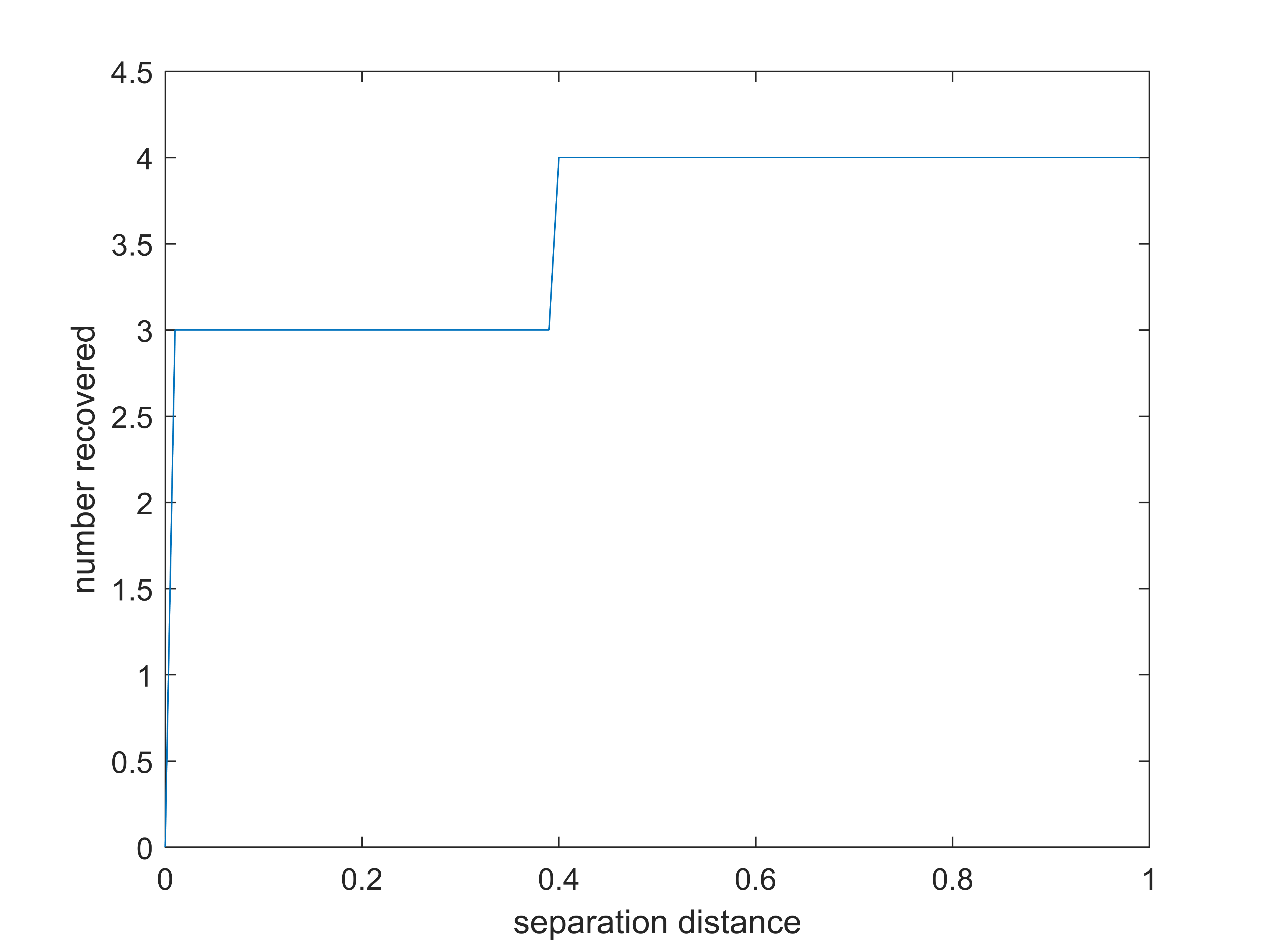
Figure 5.1: number detected by Algorithm 2 w.r.t separation distance

It shows that we can exactly recover the spectral number when they are separated more than 0.41 ($\approx 0.13\frac{\pi}{\Omega}$).

5.1 Phase transition

We know from Section 2 that the resolution limit to the number detection problem is bounded from below and above by $\frac{C_{1}}{\Omega}(\frac{\sigma}{m_{\min}})^{\frac{1}{2n-2}}$ and $\frac{C_{2}}{\Omega}(\frac{\sigma}{m_{\min}})^{\frac{1}{2n-2}}$ respectively for some constants $C_{1},C_{2}$. We shall demonstrate that this implies a phase transition phenomenon for the number detection. Precisely, recall that the super-resolution factor is $SRF=\frac{\pi}{d_{\min}\Omega}$ and the signal-to-noise ratio is $SNR=\frac{m_{\min}}{\sigma}$. From the two bounds for the resolution limit, we can draw the conclusion that exact number detection is guaranteed if

$$\log(SNR)>(2n-2)\log(SRF)+(2n-2)\log\frac{C_{1}}{\pi},$$

and may fail if

$$\log(SNR)<(2n-2)\log(SRF)+(2n-2)\log\frac{C_{2}}{\pi}.$$

As a consequence, we can see that in the parameter space of $\log SNR-\log SRF$, there exist two lines both with slope $2n-2$ such that the number detection is successful for cases above the first line and unsuccessful for cases below the second. In the intermediate region between the two lines, the number detection can be either successful or unsuccessful from case to case. This is clearly demonstrated in the numerical experiments below.

We fix $\Omega=1$ and consider $n$ line spectra equally spaced in $\big{[}-\frac{(n-1)\pi}{2},\frac{(n-1)\pi}{2}\big{]}$ by $d_{\min}$ with amplitudes $a_{j}$, and the noise level is $\sigma$. We perform 5000 random experiments (the randomness is in the choice of $(d_{\min},\sigma,y_{j},a_{j})$) to detect the number based on Algorithm 2. Figure 5.2 shows the results for $n=2,4$ respectively. In each case, two lines of slope $2n-2$ strictly separate the blue points (successful recoveries) and red points (unsuccessful recoveries) and in-between is the phase transition region.

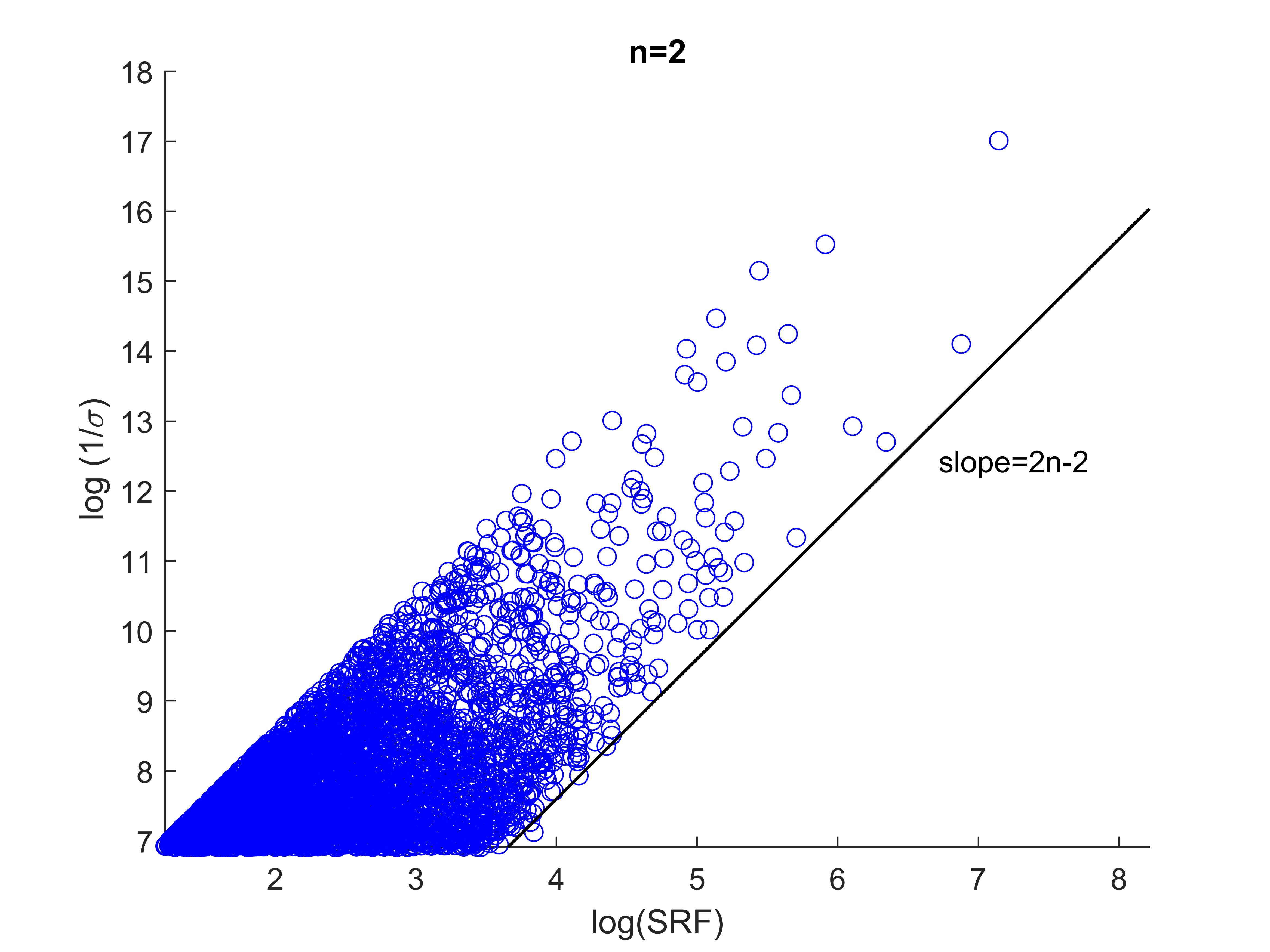
(a) detection success

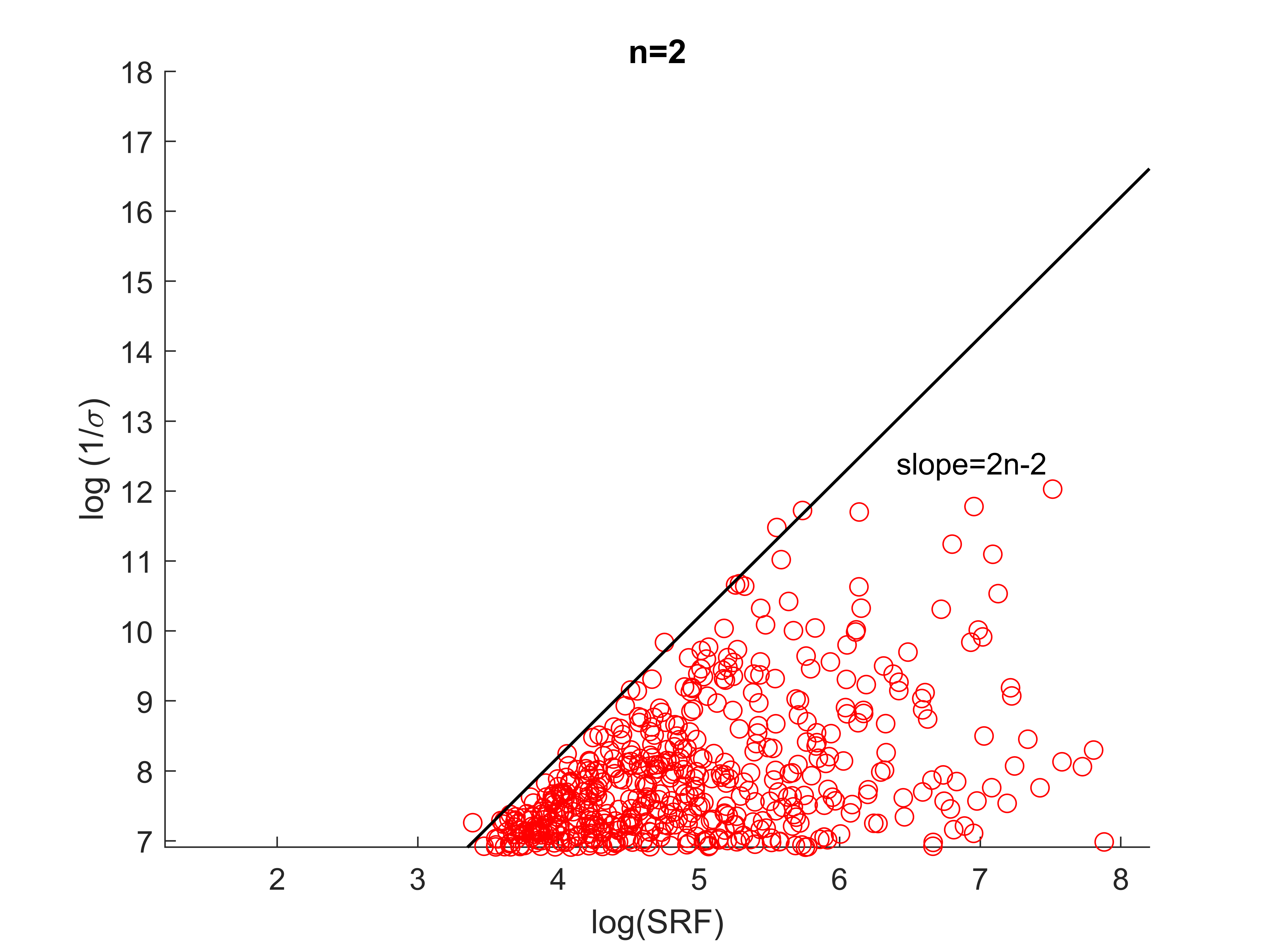
(b) detection fail

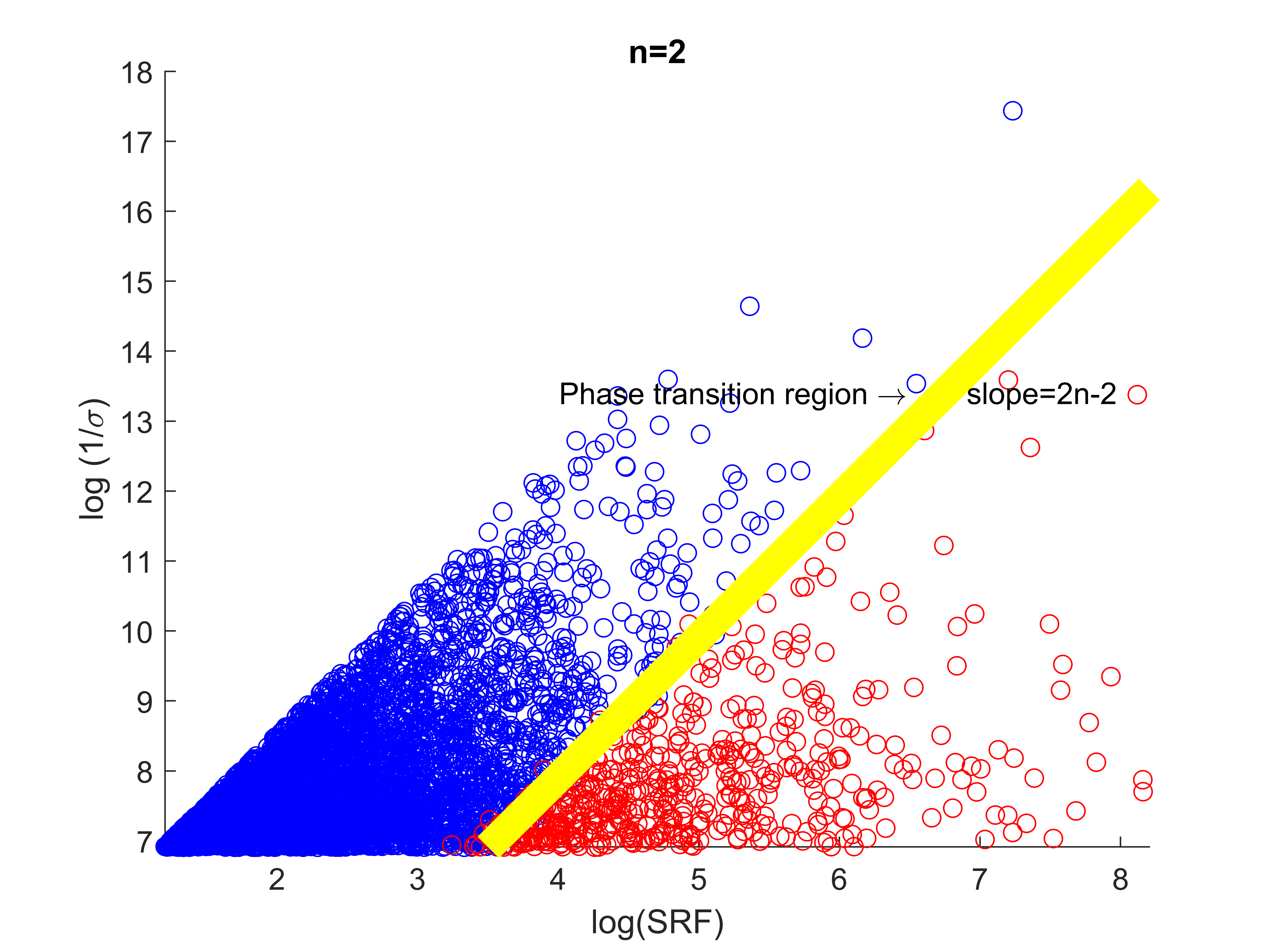
(c) phase transition region

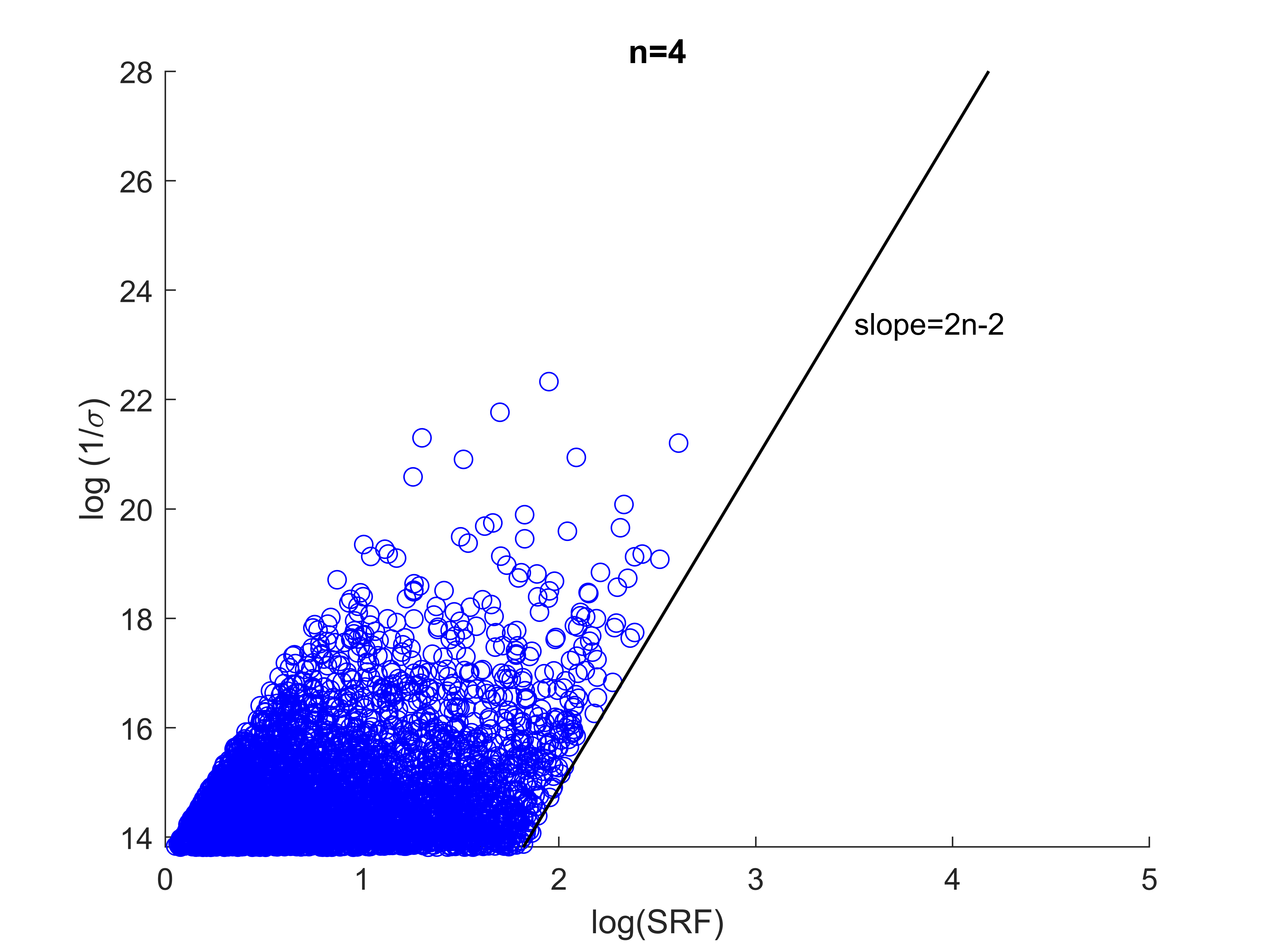
(d) detection success

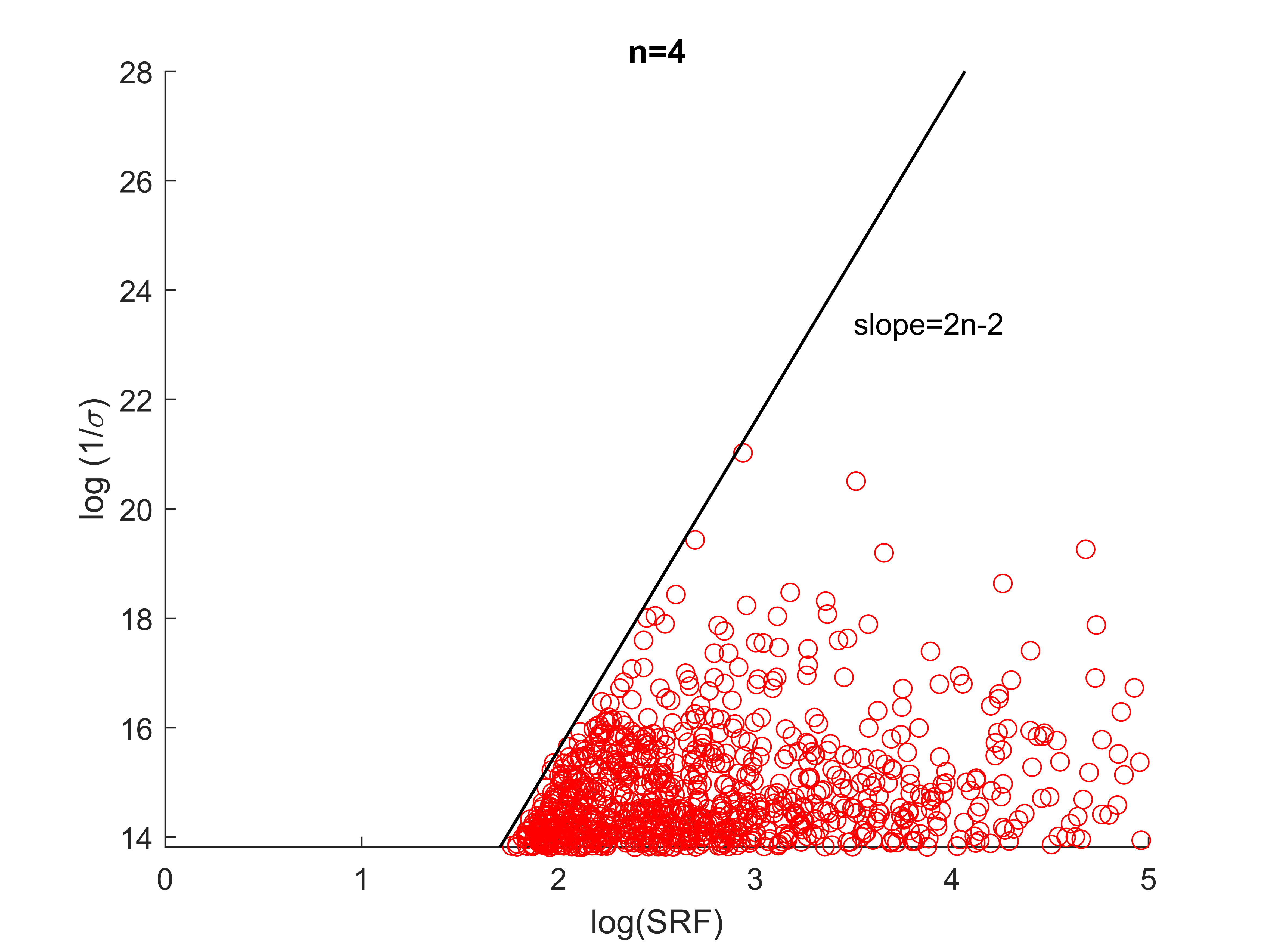
(e) detection fail

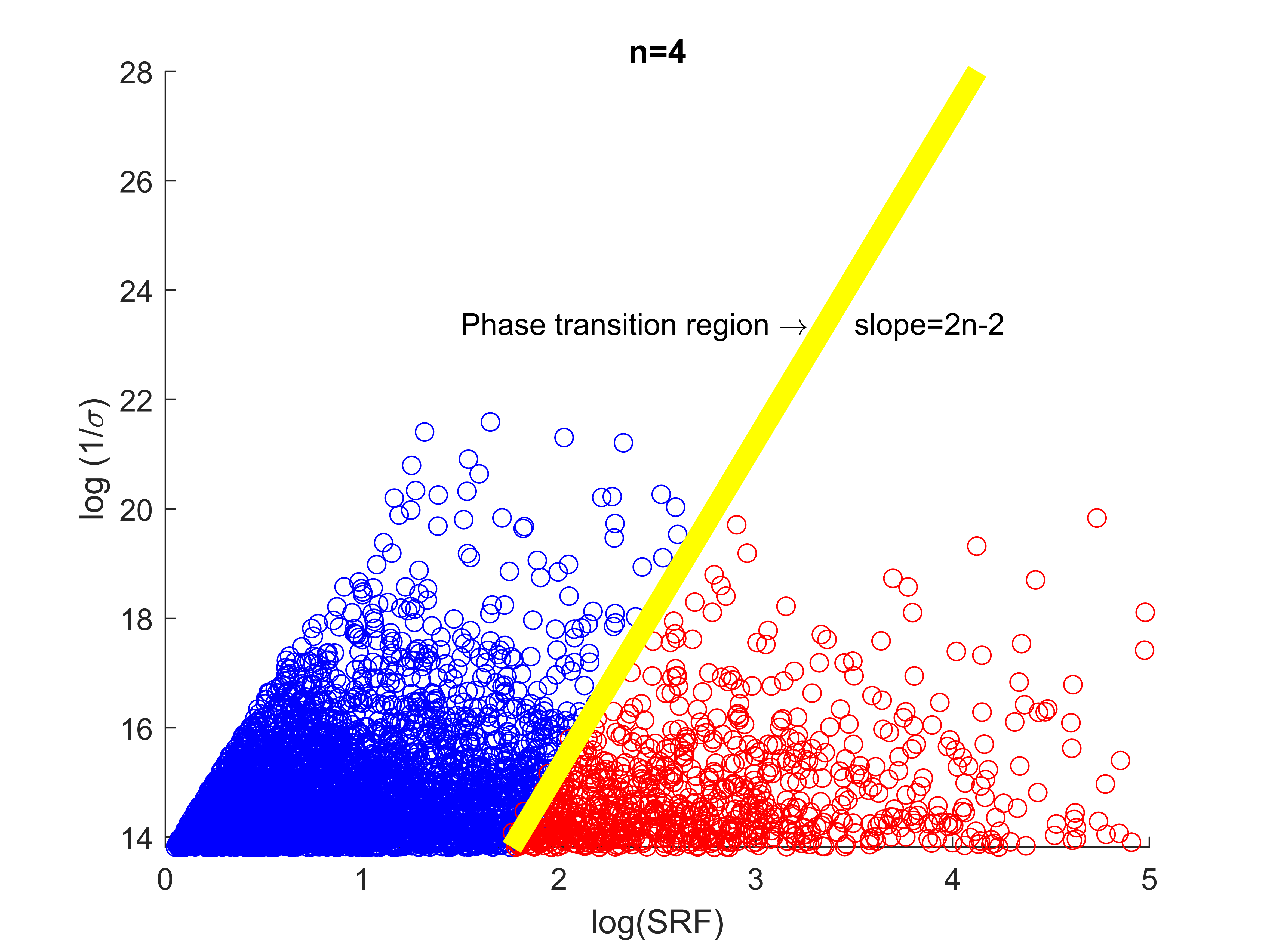
(f) phase transition region

Figure 5.2: Plots of the successful and the unsuccessful number detection by Algorithm 2 depending on the relation between $\log(SRF)$ and $\log(\frac{1}{\sigma})$. (a) illustrates that two spectra can be exactly detected if $\log(\frac{1}{\sigma})$ is above a line of slope $2$ in the parameter space. Conversely, for the same case, (b) shows that the number detection fails if $\log(\frac{1}{\sigma})$ falls below another line of slope $2$. (f) highlights the phase transition region (the yellow region) which is bounded by the black slashes in (a) and (b). (d),(e) and (f) illustrate parallel results for four spectra.

For the support recovery problem, as is shown in Section 2, the lower and upper bounds for the computational resolution limit $\mathcal{D}_{supp}$ imply a phase transition phenomenon. Similar to the number detection, we see that in the parameter space of $\log SNR-\log SRF$, there exist two lines both with slope $2n-1$ such that the support recovery is successful for cases above the first line and unsuccessful for cases below the second. This phase transition phenomenon has been demonstrated numerically using the Matrix Pencil method in [6]. Especially, in Section 3 of [6], the authors performed 15000 random experiments and showed that a line of slope $2n-1$ in the parameter space of $\log(\frac{1}{\sigma})-\log SRF$ separates the successful recoveries and the failed recoveries. Such phase transition phenomenon was also demonstrated numerically in the multi-clumps setting using the MUSIC and ESPRIT algorithms [31, 29, 30].

6 Conclusion

In this paper, we introduced two resolution limits for the number detection and the support recovery respectively in the LSE problem. We quantitatively characterized the two limits by establishing their sharp upper and lower bounds for a cluster of spectra which are bounded by multiple of Rayleigh limit. We developed sweeping singular-value-thresholding algorithm for the number detection problem and provided a theoretical analysis. We further applied the algorithm to demonstrate the phase transition phenomenon in the number detection problem. The results offer a starting point for several interesting topics in the future research. First, one may extend the study to multiple clusters and design a fast and efficient algorithm to take advantage of the separation of clusters. Second, one may extend the study to higher dimensions. And finally one may extend the study to multiple measurements to gain better resolution limits.

7 Appendix

In this Appendix, we present some inequalities that are used in this paper. We first recall the following Stirling approximation of factorial

$$\sqrt{2\pi}n^{n+\frac{1}{2}}e^{-n}\leq n!\leq en^{n+\frac{1}{2}}e^{-n},$$ (7.1)

which will be used frequently in subsequent derivation.

Lemma 7.1.

For $n\geq 2$, we have

$$\frac{(n-1)^{2n-1}}{(2n-2)!}\leq\frac{\sqrt{n-1}}{2\sqrt{\pi}}(\frac{e}{2})^{2n-2},\quad\frac{n^{2n+1}}{(2n-1)!}\leq\frac{en^{2}}{2\sqrt{\pi(n-\frac{1}{2})}}(\frac{e}{2})^{2n-1}.$$

Proof: By (7.1),

$$\frac{(n-1)^{2n-1}}{(2n-2)!}\leq\frac{(n-1)^{2n-1}}{\sqrt{2\pi}(2n-2)^{2n-2+\frac{1}{2}}e^{-(2n-2)}}=\frac{\sqrt{n-1}}{2\sqrt{\pi}}(\frac{e}{2})^{2n-2},$$

$$\frac{n^{2n+1}}{(2n-1)!}\leq\frac{n^{2n+1}}{\sqrt{2\pi}(2n-1)^{2n-1+\frac{1}{2}}e^{-(2n-1)}}\leq\frac{n^{2}}{2\sqrt{\pi(n-\frac{1}{2})}}(\frac{e}{2})^{2n-1}\frac{n^{2n-1}}{(n-\frac{1}{2})^{2n-1}}\leq\frac{en^{2}}{2\sqrt{\pi(n-\frac{1}{2})}}(\frac{e}{2})^{2n-1}.$$

Lemma 7.2.

Let $\zeta(n)$ and $\xi(n-1)$ be defined as in (3.3). For $n\geq 2$, we have

$$\Big{(}\frac{2\sqrt{2n-1}}{\zeta(n)\xi(n-1)}\Big{)}^{\frac{1}{2n-2}}\leq\frac{4.4e}{2n-1}.$$

Proof: For $n=2,3,4$, it is easy to check that the above inequality holds. Using (7.1), we have for odd $n\geq 5$,

$$\zeta(n)\xi(n-1)=(\frac{n-1}{2}!)^{2}\frac{(\frac{n-3}{2}!)^{2}}{4}\geq\pi^{2}(\frac{n-1}{2})^{n}(\frac{n-3}{2})^{n-2}e^{-(2n-4)}$$

$$= (n-\frac{1}{2})^{2n-2}\frac{\pi^{2}(\frac{n-1}{2})^{n}(\frac{n-3}{2})^{n-2}e^{-(2n-4)}}{(n-\frac{1}{2})^{2n-2}}=\pi^{2}e^{2}(\frac{n-\frac{1}{2}}{2e})^{2n-2}\frac{(n-1)^{n}(n-3)^{n-2}}{(n-\frac{1}{2})^{2n-2}}$$

$$= \pi^{2}e^{2}(\frac{n-\frac{1}{2}}{2e})^{2n-2}(\frac{n-1}{n-\frac{1}{2}})^{n}(\frac{n-3}{n-\frac{1}{2}})^{n-2}\geq 0.048(e\pi)^{2}(\frac{n-\frac{1}{2}}{2e})^{2n-2},\quad\Big{(}\text{since $n\geq 5$}\Big{)}$$

and for even $n\geq 6$,

$$\zeta(n)\xi(n-1)=(\frac{n}{2})!(\frac{n-2}{2})!\frac{(\frac{n-2}{2})!(\frac{n-4}{2})!}{4}\geq\pi^{2}(\frac{n}{2})^{\frac{n+1}{2}}(\frac{n-2}{2})^{n-1}(\frac{n-4}{2})^{\frac{n-3}{2}}e^{-(2n-4)}$$

$$= (n-\frac{1}{2})^{2n-2}\frac{\pi^{2}(\frac{n}{2})^{\frac{n+1}{2}}(\frac{n-2}{2})^{n-1}(\frac{n-4}{2})^{\frac{n-3}{2}}e^{-(2n-4)}}{(n-\frac{1}{2})^{2n-2}}=\pi^{2}e^{2}(\frac{n}{2e})^{2n-2}\frac{n^{\frac{n+1}{2}}(n-2)^{n-1}(n-4)^{\frac{n-3}{2}}}{(n-\frac{1}{2})^{2n-2}}$$

$$> 0.048(e\pi)^{2}(\frac{n-\frac{1}{2}}{2e})^{2n-2}.$$

Therefore, for all $n\geq 5$,

$$\Big{(}\frac{2\sqrt{2n-1}}{\zeta(n)\xi(n-1)}\Big{)}^{\frac{1}{2n-2}}\leq\frac{2e}{n-\frac{1}{2}}\Big{(}\frac{2\sqrt{2n-1}}{0.048(e\pi)^{2}}\Big{)}^{\frac{1}{2n-2}}\leq\frac{2.2e}{n-\frac{1}{2}}=\frac{4.4e}{2n-1}.$$

Lemma 7.3.

Let $\zeta(n)$ and $\lambda(n)$ be defined in (3.3) and (3.8) respectively. For $n\geq 2$, we have

$$\Big{(}\frac{8\sqrt{2n}}{\zeta(n)\lambda(n)}\Big{)}^{\frac{1}{2n-1}}\leq\frac{5.88e}{2n}.$$

Proof: For $n=2,3,4,5$, the inequality follows from direct calculation. By the Stirling approximation (7.1), we have for even $n\geq 6$,

$$\zeta(n)\lambda(n)=\zeta(n)\xi(n-2)\leq(\frac{n}{2})!(\frac{n-2}{2})!\frac{(\frac{n-4}{2}!)^{2}}{4}=\pi^{2}(\frac{n}{2})^{\frac{n+1}{2}}(\frac{n-2}{2})^{\frac{n-1}{2}}(\frac{n-4}{2})^{n-3}e^{-(2n-5)}$$

$$= n^{2n-1}\frac{\pi^{2}(\frac{n}{2})^{\frac{n+1}{2}}(\frac{n-2}{2})^{\frac{n-1}{2}}(\frac{n-4}{2})^{n-3}e^{-(2n-5)}}{n^{2n-1}}=(\frac{n}{2e})^{2n-1}\frac{\pi^{2}e^{4}2^{2}}{n^{2}}\frac{(n)^{\frac{n+1}{2}}(n-2)^{\frac{n-1}{2}}(n-4)^{n-3}}{n^{2n-3}}$$

$$\geq (\frac{n}{2e})^{2n-1}\frac{4\pi^{2}}{en^{2}},$$

and for odd $n\geq 7$,

$$\zeta(n)\lambda(n)=\zeta(n)\xi(n-2)=(\frac{n-1}{2}!)^{2}\frac{(\frac{n-3}{2})!(\frac{n-5}{2})!}{4}\geq\pi^{2}(\frac{n-1}{2})^{n}(\frac{n-3}{2})^{\frac{n-2}{2}}(\frac{n-5}{2})^{\frac{n-4}{2}}e^{-(2n-6)}$$

$$= n^{2n-1}\frac{\pi^{2}(\frac{n-1}{2})^{n}(\frac{n-3}{2})^{\frac{n-2}{2}}(\frac{n-5}{2})^{\frac{n-4}{2}}e^{-(2n-6)}}{n^{2n-1}}=(\frac{n}{2e})^{2n-1}\frac{\pi^{2}e^{5}2^{2}}{n^{2}}\frac{(n-1)^{n}(n-3)^{\frac{n-2}{2}}(n-5)^{\frac{n-4}{2}}}{n^{2n-3}}$$

$$\geq (\frac{n}{2e})^{2n-1}\frac{4\pi^{2}}{n^{2}}.$$

Therefore, for all $n\geq 6$,

$$\Big{(}\frac{8\sqrt{2n}}{\zeta(n)\lambda(n)}\Big{)}^{\frac{1}{2n-1}}\leq\frac{2e}{n}\Big{(}\frac{en^{2}8\sqrt{2n}}{4\pi^{2}}\Big{)}^{\frac{1}{2n-1}}\leq\frac{2.94e}{n}=\frac{5.88e}{2n}.$$

Lemma 7.4.

Let $\zeta(n)$ is defined as in (3.3). For $n\geq 2$, we have

$$\frac{(2n)^{2n-\frac{3}{2}}}{\zeta(n)(n-2)!}\leq 2^{3n-3}e^{2n}\pi^{-\frac{3}{2}}.$$

Proof: By the Stirling approximation formula (7.1), when $n$ is odd and $n\geq 3$, we have

$$\frac{(2n)^{2n-\frac{3}{2}}}{\zeta(n)(n-2)!}=\frac{(2n)^{2n-\frac{3}{2}}}{(\frac{n-1}{2}!)^{2}(n-2)!}\leq\frac{(2n)^{2n-\frac{3}{2}}}{(\sqrt{2\pi})^{3}(\frac{n-1}{2})^{n}(n-2)^{n-2+\frac{1}{2}}e^{-(2n-3)}}$$

$$\leq \frac{2^{3n-\frac{3}{2}}e^{2n}}{(e\sqrt{2\pi})^{3}}\frac{n^{n}n^{n-\frac{3}{2}}}{(n-1)^{n}(n-2)^{n-\frac{3}{2}}}\leq\frac{2^{3n-3}e^{2n}}{(\sqrt{\pi})^{3}}$$

When $n$ is even and $n\geq 4$, we have

$$\frac{(2n)^{2n-\frac{3}{2}}}{\zeta(n)(n-2)!}=\frac{(2n)^{2n-\frac{3}{2}}}{(\frac{n}{2})!(\frac{n-2}{2})!(n-2)!}\leq\frac{(2n)^{2n-\frac{3}{2}}}{(\sqrt{2\pi})^{3}(\frac{n}{2})^{\frac{n+1}{2}}(\frac{n-2}{2})^{\frac{n-1}{2}}(n-2)^{n-2+\frac{1}{2}}e^{-(2n-3)}}$$

$$\leq \frac{2^{3n-\frac{3}{2}}e^{2n}}{(e\sqrt{2\pi})^{3}}\frac{(n)^{\frac{n+1}{2}}(n)^{\frac{n-1}{2}}(n)^{n-\frac{3}{2}}}{n^{\frac{n+1}{2}}(n-2)^{\frac{n-1}{2}}(n-2)^{n-\frac{3}{2}}}\leq\frac{2^{3n-3}e^{2n}}{(\sqrt{\pi})^{3}}.$$

For $n=2$, the inequality follows from direct calculation.

Lemma 7.5.

Let $\zeta(n)$ be defined as in (3.3). For $n\geq 2$, we have

$$n\Big{(}\frac{2n(n+1)}{\zeta(n)^{2}}\Big{)}^{\frac{1}{2n-2}}<3e.$$

Proof: By (7.1), when $n$ is odd and $n\geq 3$, we have

$$n\Big{(}\frac{2n(n+1)}{\zeta(n)^{2}}\Big{)}^{\frac{1}{2n-2}}=\Big{(}\frac{n^{2n-2}2n(n+1)}{(\frac{n-1}{2}!)^{4}}\Big{)}^{\frac{1}{2n-2}}\leq\Big{(}\frac{n^{2n-2}2n(n+1)}{(2\pi)^{2}(\frac{n-1}{2})^{2n}e^{-2(n-1)}}\Big{)}^{\frac{1}{2n-2}}$$

$$= 2e\Big{(}\frac{8n(n+1)}{(2\pi)^{2}(n-1)^{2}}\frac{n^{2n-2}}{(n-1)^{2n-2}}\Big{)}^{\frac{1}{2n-2}}=2e(1+\frac{1}{n-1})\Big{(}\frac{8n(n+1)}{(2\pi)^{2}(n-1)^{2}}\Big{)}^{\frac{1}{2n-2}}$$

$$< 3e\quad\Big{(}\text{since $n\geq 3$ and $\frac{8n(n+1)}{(2\pi)^{2}(n-1)^{2}}<1$}\Big{)}.$$

On the other hand, when $n$ is odd and $n\geq 4$,

$$n\Big{(}\frac{2n(n+1)}{\zeta(n)^{2}}\Big{)}^{\frac{1}{2n-2}}=\Big{(}\frac{n^{2n-2}2n(n+1)}{((\frac{n}{2})!(\frac{n-2}{2})!)^{2}}\Big{)}^{\frac{1}{2n-2}}\leq\Big{(}\frac{n^{2n-2}2n(n+1)}{(2\pi)^{2}(\frac{n}{2})^{n+1}(\frac{n-2}{2})^{n-1}e^{-2(n-1)}}\Big{)}^{\frac{1}{2n-2}}$$

$$= 2e\Big{(}\frac{8(n+1)}{(2\pi)^{2}n}\frac{n^{n-1}}{(n-2)^{n-1}}\Big{)}^{\frac{1}{2n-2}}=2e\Big{(}1+\frac{2}{n-2}\Big{)}^{\frac{1}{2}}\Big{(}\frac{8n}{(2\pi)^{2}n}\Big{)}^{\frac{1}{2n-2}}$$

$$< 3e\quad\Big{(}\text{since $n\geq 3$ and $\frac{8(n+1)}{(2\pi)^{2}n}<1$}\Big{)}.$$

For $n=2$, the inequality follows from direct calculation.

References

• [1] Hirotogu Akaike. Information theory and an extension of the maximum likelihood principle. In Selected papers of hirotugu akaike, pages 199–213. Springer, 1998.
• [2] Hirotugu Akaike. A new look at the statistical model identification. In Selected Papers of Hirotugu Akaike, pages 215–222. Springer, 1974.
• [3] Andrey Akinshin, Dmitry Batenkov, and Yosef Yomdin. Accuracy of spike-train fourier reconstruction for colliding nodes. In 2015 International Conference on Sampling Theory and Applications (SampTA), pages 617–621. IEEE, 2015.
• [4] Jean-Marc Azais, Yohann De Castro, and Fabrice Gamboa. Spike detection from inaccurate samplings. Applied and Computational Harmonic Analysis, 38(2):177–195, 2015.
• [5] Dmitry Batenkov, Laurent Demanet, Gil Goldman, and Yosef Yomdin. Conditioning of partial nonuniform fourier matrices with clustered nodes. SIAM Journal on Matrix Analysis and Applications, 41(1):199–220, 2020.
• [6] Dmitry Batenkov, Gil Goldman, and Yosef Yomdin. Super-resolution of near-colliding point sources. Information and Inference: A Journal of the IMA, 05 2020. iaaa005.
• [7] Emmanuel J. Candès and Carlos Fernandez-Granda. Super-resolution from noisy data. Journal of Fourier Analysis and Applications, 19(6):1229–1254, 2013.
• [8] Emmanuel J. Candès and Carlos Fernandez-Granda. Towards a mathematical theory of super-resolution. Communications on Pure and Applied Mathematics, 67(6):906–956, 2014.
• [9] Weiguo Chen, Kon Max Wong, and James P Reilly. Detection of the number of signals: A predicted eigen-threshold approach. IEEE Transactions on Signal Processing, 39(5):1088–1098, 1991.
• [10] Yuejie Chi and Maxime Ferreira Da Costa. Harnessing sparsity over the continuum: Atomic norm minimization for superresolution. IEEE Signal Processing Magazine, 37(2):39–57, 2020.
• [11] Laurent Demanet and Nam Nguyen. The recoverability limit for superresolution via sparsity. arXiv preprint arXiv:1502.01385, 2015.
• [12] Arnold J Den Dekker. Model-based optical resolution. In Quality Measurement: The Indispensable Bridge between Theory and Reality (No Measurements? No Science! Joint Conference-1996: IEEE Instrumentation and Measurement Technology Conference and IMEKO Tec, volume 1, pages 441–446. IEEE, 1996.
• [13] Arnold Jan Den Dekker and A Van den Bos. Resolution: a survey. JOSA A, 14(3):547–557, 1997.
• [14] Quentin Denoyelle, Vincent Duval, and Gabriel Peyré. Support recovery for sparse super-resolution of positive measures. Journal of Fourier Analysis and Applications, 23(5):1153–1194, 2017.
• [15] David L. Donoho. Superresolution via sparsity constraints. SIAM journal on mathematical analysis, 23(5):1309–1331, 1992.
• [16] Vincent Duval and Gabriel Peyré. Exact support recovery for sparse spikes deconvolution. Foundations of Computational Mathematics, 15(5):1315–1355, 2015.
• [17] Carlos Fernandez-Granda. Support detection in super-resolution. In Proceedings of the 10th International Conference on Sampling Theory and Applications (SampTA 2013), pages 145–148, 2013.
• [18] Carlos Fernandez-Granda. Super-resolution of point sources via convex programming. Information and Inference: A Journal of the IMA, 5(3):251–303, 2016.
• [19] Walter Gautschi. On inverses of vandermonde and confluent vandermonde matrices. Numerische Mathematik, 4(1):117–123, 1962.
• [20] Keyong Han and Arye Nehorai. Improved source number detection and direction estimation with nested arrays and ulas using jackknifing. IEEE Transactions on Signal Processing, 61(23):6118–6128, 2013.
• [21] Thomas Lundgaard Hansen, Bernard Henri Fleury, and Bhaskar D Rao. Superfast line spectral estimation. IEEE Transactions on Signal Processing, 66(10):2511–2526, 2018.
• [22] Zhaoshui He, Andrzej Cichocki, Shengli Xie, and Kyuwan Choi. Detecting the number of clusters in n-way probabilistic clustering. IEEE Transactions on Pattern Analysis and Machine Intelligence, 32(11):2006–2021, 2010.
• [23] C Helstrom. The detection and resolution of optical signals. IEEE Transactions on Information Theory, 10(4):275–287, 1964.
• [24] Carl W Helstrom. Detection and resolution of incoherent objects by a background-limited optical system. JOSA, 59(2):164–175, 1969.
• [25] Yingbo Hua and Tapan K. Sarkar. Matrix pencil method for estimating parameters of exponentially damped/undamped sinusoids in noise. IEEE Transactions on Acoustics, Speech, and Signal Processing, 38(5):814–824, 1990.
• [26] Yingbo Hua and Tapan K Sarkar. On svd for estimating generalized eigenvalues of singular matrix pencil in noise. In 1991., IEEE International Sympoisum on Circuits and Systems, pages 2780–2783. IEEE, 1991.
• [27] DN Lawley. Tests of significance for the latent roots of covariance and correlation matrices. biometrika, 43(1/2):128–136, 1956.
• [28] Qiuwei Li and Gongguo Tang. Approximate support recovery of atomic line spectral estimation: A tale of resolution and precision. Applied and Computational Harmonic Analysis, 2018.
• [29] Weilin Li and Wenjing Liao. Stable super-resolution limit and smallest singular value of restricted fourier matrices. 2018.
• [30] Weilin Li, Wenjing Liao, and Albert Fannjiang. Super-resolution limit of the esprit algorithm. arXiv preprint arXiv:1905.03782, 2019.
• [31] Wenjing Liao and Albert C. Fannjiang. Music for single-snapshot spectral estimation: Stability and super-resolution. Applied and Computational Harmonic Analysis, 40(1):33–67, 2016.
• [32] Ping Liu and Hai Zhang. Computational resolution limit: a theory towards super-resolution. arXiv preprint arXiv:1912.05430, 2019.
• [33] Leon B Lucy. Resolution limits for deconvolved images. The Astronomical Journal, 104:1260–1265, 1992.
• [34] Leon B Lucy. Statistical limits to super resolution. Astronomy and Astrophysics, 261:706, 1992.
• [35] Ankur Moitra. Super-resolution, extremal functions and the condition number of vandermonde matrices. In Proceedings of the Forty-seventh Annual ACM Symposium on Theory of Computing, STOC ’15, pages 821–830, New York, NY, USA, 2015. ACM.
• [36] Veniamin I Morgenshtern. Super-resolution of positive sources on an arbitrarily fine grid. arXiv preprint arXiv:2005.06756, 2020.
• [37] Veniamin I. Morgenshtern and Emmanuel J. Candes. Super-resolution of positive sources: The discrete setup. SIAM Journal on Imaging Sciences, 9(1):412–444, 2016.
• [38] Athanasios Papoulis and Christodoulos Chamzas. Improvement of range resolution by spectral extrapolation. Ultrasonic Imaging, 1(2):121–135, 1979.
• [39] Clarice. Poon and Gabriel. Peyré. Multidimensional sparse super-resolution. SIAM Journal on Mathematical Analysis, 51(1):1–44, 2019.
• [40] R. Prony. Essai expérimental et analytique. J. de l’ Ecole Polytechnique (Paris), 1(2):24–76, 1795.
• [41] Lord Rayleigh. Xxxi. investigations in optics, with special reference to the spectroscope. The London, Edinburgh, and Dublin Philosophical Magazine and Journal of Science, 8(49):261–274, 1879.
• [42] Jorma Rissanen. Modeling by shortest data description. Automatica, 14(5):465–471, 1978.
• [43] Richard Roy and Thomas Kailath. Esprit-estimation of signal parameters via rotational invariance techniques. IEEE Transactions on acoustics, speech, and signal processing, 37(7):984–995, 1989.
• [44] Ralph Schmidt. Multiple emitter location and signal parameter estimation. IEEE transactions on antennas and propagation, 34(3):276–280, 1986.
• [45] Gideon Schwarz et al. Estimating the dimension of a model. The annals of statistics, 6(2):461–464, 1978.
• [46] Morteza Shahram and Peyman Milanfar. Imaging below the diffraction limit: a statistical analysis. IEEE Transactions on image processing, 13(5):677–689, 2004.
• [47] Morteza Shahram and Peyman Milanfar. Statistical analysis of achievable resolution in incoherent imaging. In Signal and Data Processing of Small Targets 2003, volume 5204, pages 1–9. International Society for Optics and Photonics, 2004.
• [48] Morteza Shahram and Peyman Milanfar. On the resolvability of sinusoids with nearby frequencies in the presence of noise. IEEE Transactions on Signal Processing, 53(7):2579–2588, 2005.
• [49] Petre Stoica and Arye Nehorai. Music, maximum likelihood, and cramer-rao bound. IEEE Transactions on Acoustics, speech, and signal processing, 37(5):720–741, 1989.
• [50] Gongguo Tang. Resolution limits for atomic decompositions via markov-bernstein type inequalities. In 2015 International Conference on Sampling Theory and Applications (SampTA), pages 548–552. IEEE, 2015.
• [51] Gongguo Tang, Badri Narayan Bhaskar, and Benjamin Recht. Near minimax line spectral estimation. IEEE Transactions on Information Theory, 61(1):499–512, 2014.
• [52] Gongguo Tang, Badri Narayan Bhaskar, Parikshit Shah, and Benjamin Recht. Compressed sensing off the grid. IEEE transactions on information theory, 59(11):7465–7490, 2013.
• [53] Mati Wax and Thomas Kailath. Detection of signals by information theoretic criteria. IEEE Transactions on acoustics, speech, and signal processing, 33(2):387–392, 1985.
• [54] Mati Wax and Ilan Ziskind. Detection of the number of coherent signals by the mdl principle. IEEE Transactions on Acoustics, Speech, and Signal Processing, 37(8):1190–1196, 1989.