Mean absolute deviations about the mean, the cut norm and taxicab correspondence analysis

Abstract

Optimization has two faces, minimization of a loss function or maximization of a gain function. We show that the mean absolute deviations about the mean, $d$, maximizes a gain function based on the power set of the individuals, and it is equal to twice the value of its cut-norm. This property is generalized to double-centered and triple-centered data sets. Furthermore, we show that among the three well known dispersion measures, standard deviation, least absolute deviation and $d$, $d$ is the most robust based on the relative contribution criterion. More importantly, we show that the computation of each principal dimension of taxicab correspondence analysis corresponds to balanced 2-blocks seriation. Examples are provided.

Key words: Mean absolute deviations about the mean; cut norm; balanced 2-blocks seriation; taxicab correspondence analysis.

1 Introduction

Optimization has two faces, minimization of a loss function or maximization of a gain function. The following two well known dispersion measures, the variance ($s^{2})$ and mean absolute deviations about the median $(LAD$), are optimal because each minimizes a different loss function

$$s^{2} = \frac{\sum_{i=1}^{n}(y_{i}-\overline{y})^{2}}{n}$$ (1)

$$\leq \frac{\sum_{i=1}^{n}(y_{i}-c)^{2}}{n}$$

and

$$LAD = \frac{\sum_{i=1}^{n}|y_{i}-median|}{n}$$ (2)

$$\leq \frac{\sum_{i=1}^{n}|y_{i}-c|}{n},$$

where $y_{1},\ y_{2,}...,y_{n}\$and $c$ represent a sample of ($n+1)$ values. To our knowledge, no optimality property is known for the mean absolute deviations about the mean defined by

$$d=\frac{\sum_{i=1}^{n}|y_{i}-\overline{y}|}{n},$$ (3)

even though it has been studied in several papers for modeling purposes by, see among others, Pham-Gia and Hung (2001), Gorard (2015), Yitzhaki and Lambert (2013). Pham-Gia and Hung (2001) and Gorard (2015) essentially compare the dispersion measures $d$ and $s$ in the statistical litterature, with their preference clearly oriented towards $d$ for its simple interpretability. While Yitzhaki and Lambert (2013) compare the statistics $d$ and $LAD$ with the Gini dispersion measure and conclude that ”The downside of using ($d$ and $LAD$) is that robustness is achieved by omitting the information on the intra-group variability”.

The following inequality $LAD\leq d\leq s$ is well known: it follows from (2) and the fact that $ns^{2}=\sum_{i=1}^{n}w_{i}^{2}-n\overline{w}^{2}\geq 0$, where $w_{i}=|y_{i}-\overline{y}|.$

$d$ is the measure of dispersion used in taxicab correspondence analysis (TCA), an L₁ variant of correspondence analysis (CA), see Choulakian (2006). An explanation for the robustness of $d$ is the boundedness of the relative contribution of a point, see Choulakian (2008a, 2008b, 2017) and Choulakian et al. (2013a, 2013b, 2014). However, this paper provides further details on $d$, relating it to cut-norm and balanced 2-blocks seriation for double-centered data. Choulakian (2017) argued that often sparse contingency tables are better visualized by TCA; here, we present an analysis of a 0-1 affinity matrix, where TCA produces a much more interpretable map than CA. We see that repetition and experience play an indispensable and illuminating role in data analysis.

This paper is organized as follows: In section 2, we show the optimality of the $d,\ s^{2}$ and $LAD$ statistics based on maximizing gain functions, but $d$ beats $s^{2}$ and $LAD$ with respect to the property of relative contribution of a point (a robustness measure used in french data analysis circles based on geometry): this results from Lemma 1, which states the fact that for a centered vector $d$ equals twice its cut-norm; sections 3 and 4 generalize the optimality result of the $d$ to double-centered and triple-centered arrays; and we conclude in section 5. Balanced 2-blocks seriation of a matrix with application to TCA is discussed in section 3.

2 Optimality of d

We construct the centered vector ${\mathbf{x}}={\mathbf{y}}-\overline{y}\ {\mathbf{1}}_{n}$, where ${\mathbf{1}}_{n}$ is composed of $n$ ones. Let $I=\left\{1,2,...,n\right\}$ and $I=S\cup\overline{S}$ a binary partition of $I$. We have

$$\sum_{i\in I}x_{i} = 0$$

$$= \sum_{i\in S}x_{i}+\sum_{i\in\overline{S}}x_{i};$$

from which we deduce

$$\sum_{i\in S}x_{i}=-\sum_{i\in\overline{S}}x_{i}.$$ (4)

We define the cut-norm of a centered vector x to be $||{\mathbf{x}||}_{\boxdot}=\max_{S}\sum_{i\in S}x_{i}=\sum_{i\in S_{opt}}x_{i}$, where $S_{opt}=\left\{i:x_{i}\geq 0\text{ for }i=1,2,...,n\right\}.$ By casting the computation of $d$ as a combinatorial maximization problem, we have the following main result describing the optimality of the $d$-statistic over all elements of the power set of $I$.

Lemma 1: (2-equal parts property) $d=2||{\mathbf{x}||}_{\boxdot}\geq 2\sum_{i\in S}x_{i}/n$    for  all  $S\subset I$.

Proof: Easily shown by using (4).

Corollary 1: $d\geq{\mathbf{x}}^{\prime}{\mathbf{u}/}n$   for  ${\mathbf{u}}\in\left\{-1,1\right\}^{n}.\vskip 12.0pt plus 4.0pt minus 4.0pt$

Proof: By defining ${\mathbf{u}}_{opt}(i)=1$ if $i\in S_{opt}$ and$\ {\mathbf{u}}_{opt}(i)=-1$ if $i\in\overline{S}_{opt}$, we get $d={\mathbf{x}}^{\prime}{\mathbf{u}}_{opt}{\mathbf{/}}n\geq{\mathbf{x}}^{\prime}{\mathbf{u}/}n.$

Corollary 2: $LAD\geq({\mathbf{y}}-median$ ${\mathbf{1}}_{n})^{\prime}{\mathbf{u}/}n$   for  ${\mathbf{u}}\in\left\{-1,1\right\}^{n}.$

Corollary 2 shows that LAD has a second optimality property. We emphasize the fact that the optimizing function in (2) is a univariate loss function of $c\in\mathbb{R}$; while the optimizing function in Corollary 2 is a multivariate gain function of ${\mathbf{u}}\in\left\{-1,1\right\}^{n}$.

There is a similar result also for the variance in (1), based on Cauchy-Schwarz inequality.

Lemma 2: $s\geq({\mathbf{y}}-\overline{y}{\mathbf{1}}_{n})^{\prime}{\mathbf{u}/}\sqrt{n}\ \$ for$\ \ {\mathbf{u}}^{\prime}{\mathbf{u}=}1{\mathbf{.}\vskip 12.0pt plus 4.0pt minus 4.0pt}$

We note that Lemmas 1 and 2 represent particular cases of Hölder inequality, see Choulakian ( (2016).

Definition 1: We define the relative contribution of an element $y_{i}$ to $d,$ $LAD$ and $s^{2}$, respectively, to be

$$RC_{d}(y_{i})=\frac{|y_{i}-\overline{y}|}{n\ d},$$

$$RC_{s^{2}}(y_{i})=\frac{|y_{i}-\overline{y}|^{2}}{n\ s^{2}},$$

$$RC_{LAD}(y_{i})=\frac{|y_{i}-median|}{n\ AD}.$$

Then the following inequalities are true

$$0\leq RC_{d}(y_{i})\leq 0.5,$$

$$0\leq RC_{s^{2}}(y_{i})<1,$$

$$0\leq RC_{LAD}(y_{i})\leq 1;$$

from which we conclude that the most robust dispersion measure among the three dispersion measures, based on the relative contribution criterion, is $d.$

We note that the inequality, $0\leq RC_{s^{2}}(y_{i})<1,$ is a weaker variant of Laguerre-Samuelson inequality; see for instance, Jensen (1999), whose MS thesis presents nine different proofs.

We have

Definition 2: An element $x_{i}=y_{i}-\overline{y}$ is a heavyweight if $RC_{d}(y_{i})=0.5;$ that is, $|x_{i}|=|y_{i}-\overline{y}|=nd/2.\vskip 12.0pt plus 4.0pt minus 4.0pt$

We note that a heavyweight element attains the upper bound of $RC_{d}(y_{i}),$ but it never attains the upper bound of $RC_{s^{2}}(y_{i})$ and $RC_{LAD}(y_{i}).$

3 2-way interactions of a correspondence matrix

Let ${\mathbf{P}=(}p_{ij})\$be a correspondence matrix; that is, $p_{ij}\geq 0$ for $i\in I$ and $j\in J=\left\{1,2,...,m\right\}$ and $\sum_{j=1}^{m}\sum_{i=1}^{n}p_{ij}=1.$ As usual, we define $p_{i\ast}=\sum_{j=1}^{m}p_{ij}$ and $p_{\ast j}=\sum_{i=1}^{n}p_{ij}$. Let ${\mathbf{P}}_{1}{\mathbf{=}(}x_{ij}=p_{ij}-p_{i\ast}p_{\ast j})$ for $i\in I$ and $j\in J;$ then ${\mathbf{P}}_{1}$ represents the residual matrix of ${\mathbf{P}}$ with respect to the independence model $(p_{i\ast}p_{\ast j})$. In the jargon of statistics, the cell $x_{ij}$ represents the multiplicative 2-way interaction of the cell ($i,j)\in I\times J.$ ${\mathbf{P}}_{1}$ is double-centered

$${\mathbf{P}}_{1}{\mathbf{1}}_{m}={\mathbf{0}}_{n}\text{\ \ \ \ \ and\ \ \ \ \ }{\mathbf{P}}_{1}{\mathbf{}{\prime}1}_{n}={\mathbf{0}}_{n}.$$ (5)

From (5) we get

$$\sum_{i\in S}x_{ij} = -\sum_{i\in\overline{S}}x_{ij}\text{\ \ \ \ for }j\in J,$$ (6)

$$\sum_{j\in T}x_{ij} = -\sum_{j\in\overline{T}}x_{ij}\text{\ \ \ \ for }i\in I,$$ (7)

for $T\subset J.$ From (6) and (7), we get

$$\sum_{j\in T}\sum_{i\in S}x_{ij} = -\sum_{j\in T}\sum_{i\in\overline{S}}x_{ij},$$ (8)

$$= -\sum_{i\in S}\sum_{j\in\overline{T}}x_{ij}$$ (9)

$$= \sum_{i\in\overline{S}}\sum_{j\in\overline{T}}x_{ij}.$$ (10)

We define the cut-norm of ${\mathbf{P}}_{1}$ to be

$$||{\mathbf{P}}_{1}{\mathbf{|}|}_{\boxdot}=\max_{S,T}\sum_{j\in T}\sum_{i\in S}x_{ij}=\sum_{j\in T_{opt}}\sum_{i\in S_{opt}}x_{ij}.$$

The cut-norm $||{\mathbf{P}}_{1}{\mathbf{|}|}_{\boxdot}$ is a well known quantity in theoretical computer science, because of its relationship to the famous Grothendieck inequality, which is based on $||{\mathbf{P}}_{1}||_{\infty\rightarrow 1},$ see among others Khot and Naor (2012).

The matrix ${\mathbf{P}}_{1}$ can be considered as the starting point in taxicab correspondence analysis, an L₁ variant of correspondence analysis , see Choulakian (2006). The optimization criterion in TCA of ${\mathbf{P}}$ or ${\mathbf{P}}_{1}$ is based on taxicab matrix norm, which is a combinatorial optimization problem

$$\delta_{1} = ||{\mathbf{P}}_{1}||_{\infty\rightarrow 1}=||{\mathbf{P}}_{1}^{\prime}||_{\infty\rightarrow 1}$$ (11)

$$= \max_{{\mathbf{u}\in\mathbb{R}}^{m}}\frac{\left|\left|{\mathbf{P}}_{1}{\mathbf{u}}\right|\right|_{1}}{\left|\left|{\mathbf{u}}\right|\right|_{\infty}}=\max_{{\mathbf{v}\in\mathbb{R}}^{n}}\ \frac{\left|\left|{\mathbf{P}}_{1}{\mathbf{}{\prime}v}\right|\right|_{1}}{\left|\left|{\mathbf{v}}\right|\right|_{\infty}}=\max_{{\mathbf{u}\in\mathbb{R}}^{m},{\mathbf{v}\in\mathbb{R}}^{n}}\frac{{\mathbf{v}}^{\prime}{\mathbf{P}}_{1}{\mathbf{u}}}{\left|\left|{\mathbf{u}}\right|\right|_{\infty}\left|\left|{\mathbf{v}}\right|\right|_{\infty}},$$

$$= \max||{\mathbf{P}}_{1}{\mathbf{u}||}_{1}\ \ \text{subject to }{\mathbf{u}}\in\left\{-1,+1\right\}^{m},$$

$$= \max||{\mathbf{P}}_{1}{\mathbf{}{\prime}v||}_{1}\ \ \text{subject to }{\mathbf{v}}\in\left\{-1,+1\right\}^{n},$$

$$= \max{\mathbf{v}}^{\prime}{\mathbf{P}}_{1}{\mathbf{u}}\text{ \ subject to \ }{\mathbf{u}}\in\left\{-1,+1\right\}^{m},{\mathbf{v}}\in\left\{-1,+1\right\}^{n},$$

$$= {\mathbf{v}}_{1}^{\prime}{\mathbf{P}}_{1}{\mathbf{u}}_{1}.$$ (12)

In data analysis, the vectors ${\mathbf{v}}_{1}$ and ${\mathbf{u}}_{1}$ are interpreted as taxicab principal axes and $\delta_{1}$ as first taxicab dispersion. So we can compute the projection of the rows (resp. the columns) of ${\mathbf{P}}_{1}$ on the taxicab principal axis ${\mathbf{u}}_{1}$ (resp. ${\mathbf{v}}_{1})$ to be

$${\mathbf{a}}_{1} = {\mathbf{P}}_{1}{\mathbf{u}}_{1}$$ (13)

$${\mathbf{b}}_{1} = {\mathbf{P}}_{1}^{\prime}{\mathbf{v}}_{1}.$$ (14)

Equation (12) implies

$${\mathbf{v}}_{1} = sign({\mathbf{a}}_{1}),$$ (15)

$${\mathbf{u}}_{1} = sign({\mathbf{b}}_{1}),$$ (16)

named transition formulas, see Choulakian (2006, 2016). We also note the following identities

$${\mathbf{1}}_{n}^{\prime}{\mathbf{a}}_{1} = 0\text{ \ \ \ and \ \ }\delta_{1}=||{\mathbf{a}}_{1}||_{1},$$ (17)

$${\mathbf{1}}_{m}^{\prime}{\mathbf{b}}_{1} = 0\text{ \ \ \ and \ \ }\delta_{1}=||{\mathbf{b}}_{1}||_{1}.$$ (18)

Using the above results, we get the following

Lemma 3: (4-equal parts property) The norm $\delta_{1}=||{\mathbf{P}}_{1}||_{\infty\rightarrow 1}=4||{\mathbf{P}}_{1}{\mathbf{|}|}_{\boxdot}\geq 4\sum_{j\in T}\sum_{i\in S}x_{ij}.\vskip 12.0pt plus 4.0pt minus 4.0pt$

In data analysis, Lemma 3 implies balanced 2-blocks seriation of ${\mathbf{P}}_{1};$ see example 1. The subsets $T_{opt}$ and $S_{opt}$ are positively associated and $||{\mathbf{P}}_{1}{\mathbf{|}|}_{\boxdot}=\sum_{j\in T_{opt}}\sum_{i\in S_{opt}}x_{ij}$; similarly the subsets $\overline{T}_{opt}$ and $\overline{S}_{opt}$ are positively associated and $||{\mathbf{P}}_{1}{\mathbf{|}|}_{\boxdot}=\sum_{j\in\overline{T}_{opt}}\sum_{i\in\overline{S}_{opt}}x_{ij}.$ While the subsets $\overline{T}_{opt}$ and $S_{opt}$ are negatively associated and $||{\mathbf{P}}_{1}{\mathbf{|}|}_{\boxdot}=-\sum_{j\in\overline{T}_{opt}}\sum_{i\in S_{opt}}x_{ij};$ similarly the subsets $T_{opt}$ and $\overline{S}_{opt}$ are negatively associated and $||{\mathbf{P}}_{1}{\mathbf{|}|}_{\boxdot}=-\sum_{j\in T_{opt}}\sum_{i\in\overline{S}_{opt}}x_{ij}.$ Liiv (2010) presents an interesting overview of seriation.

Using Definition 2, we get

Definition 3: The relative contribution of the row $i$ to $\delta_{1}$ (respectively of the column $j$ to $\delta_{1}$) is

$$RC_{{}_{1}}(\mathop{\mathrm{r}ow}\ i)=\frac{|{\mathbf{a}}_{1}(i)|}{\delta_{1}}\text{ and }RC_{{}_{1}}(\mathop{\mathrm{c}ol}\ j)=\frac{|{\mathbf{b}}_{1}(i)|}{\delta_{1}}.$$

We have

$$0\leq RC_{1}(\mathop{\mathrm{r}ow}\ i)\text{ and }RC_{1}(\mathop{\mathrm{c}ol}\ j)\leq 0.5.$$

Definition 4: a) On the first taxicab principlal axis the row $i$ is heavyweight if $RC_{1}(\mathop{\mathrm{r}ow}\ i)=0.5,$ and the column $j$ is heavyweight if $RC_{1}(\mathop{\mathrm{c}ol}\ j)=0.5.$

b) On the first taxicab principlal axis the cell $(i,j)$ is heavyweight if and only if both row $i$ and column $j$ are heavyweights; and in this case $RC_{1}(p_{ij}-p_{i\ast}p_{\ast j})=\frac{|p_{ij}-p_{i\ast}p_{\ast j}|}{\delta_{1}}=0.25.\vskip 12.0pt plus 4.0pt minus 4.0pt$

For an application of Definitions 3 and 4 see Choulakian (2008a).

Using Wedderburn’s rank-1 reduction rule, see Choulakian (2016), we construct the 2nd residual matrix ${\mathbf{P}}_{2}={\mathbf{(}}x_{ij}=p_{ij}-p_{i\ast}p_{\ast j}-\frac{a_{1}(i)b_{1}(j)}{\sigma_{1}}),$ and repeat the above procedure. After $k=rank({\mathbf{P}}_{1})$ iterations, we decompose the correspondence matrix ${\mathbf{P}}$ into $(k+1)$ bilinear parts

$$p_{ij}=p_{i\ast}p_{\ast j}+\sum_{\alpha=1}^{k}\frac{a_{\alpha}(i)b_{\alpha}(j)}{\delta_{\alpha}},$$

named taxicab singular value decomposition; which can be rewritten, similar to data reconstruction formula in correspondence analysis (CA), as

$$p_{ij}=p_{i\ast}p_{\ast j}(1+\sum_{\alpha=1}^{k}\frac{f_{\alpha}(i)g_{\alpha}(j)}{\delta_{\alpha}}),$$

where $f_{\alpha}(i)=a_{\alpha}(i)/p_{i\ast}$ and $g_{\alpha}(j)=b_{\alpha}(j)/p_{\ast j}.$ CA and TCA satisfy an important invariance property: columns (or rows) with identical profiles (conditional probabilities) receive identical factor scores $g_{\alpha}(j)$ (or $f_{\alpha}(i))$. The factor scores are used in the graphical displays. Moreover, merging of identical profiles does not change the results of the data analysis: This is named the principle of equivalent partitioning by Nishisato (1984); it includes the famous invariance property named principle of distributional equivalence, on which Benzécri (1973) developed CA.

In the next subsections we shall present two examples, where taxicab correspondence analysis (TCA) is applied. The first data set is a small contingency table taken from Beh and Lombardo (2014), for which we present the details of the computation explaing the contents of section 3. The second data set is a networks affinity matrix from Faust (2005). For both data sets we compare CA and TCA maps.

The theory of CA can be found, among others, in Benzécri (1973, 1992), Greenacre (1984), Gifi (1990), Le Roux and Rouanet (2004), Murtagh (2005), and Nishisato (2007); the recent book, authored by Beh and Lombardi (2014), presents a panoramic review of CA and related methods.

3.1 Selikoff’s asbestos data set

Table 1, taken from Beh and Lombardo (2014), is a contingency table Y of size $5\times 4$ cross-classifying 1117 New York workers with occupational exposure to asbestos; the workers are classified according to the number of exposure in years (five categories) and the asbestos grade diagnosed (four categories). Figures 1 and 2 display the maps obtained by CA and TCA: almost no difference between them. Here, we present the details of the computation for TCA. Table 2 presents the residual correspondence table ${\mathbf{P}}_{1}$ with respect to the independence model, where we see diagonal 2-blocks seriation of ${\mathbf{P}}_{1}$ with$:$ $S_{opt}=\left\{\text{row1, row2}\right\}$ is positively associated with $T_{opt}=\left\{\text{column1}\right\}$ and the cut-norm $||{\mathbf{P}}_{1}{\mathbf{|}|}_{\boxdot}=(0.1181+0.0151)=0.1332;$ similarly, $\overline{S}_{opt}=\left\{\text{row3, row4, row5}\right\}$ is positively associated with
$\overline{T}_{opt}=\left\{\text{column2, column3, column4}\right\}$ and $||{\mathbf{P}}_{1}{\mathbf{|}|}_{\boxdot}=\sum_{j\in\overline{T}_{opt}}\sum_{i\in\overline{S}_{opt}}x_{ij}=0.0087+...+0.0202=0.1332.\$Note that the elements in the positively associated diagonal blocks have in majority positive values; while the elements in the negatively associated diagonal blocks have in majority negative values. The last three columns and the last three rows of Table 2 display principal axes (${\mathbf{v}}_{1}$ and ${\mathbf{u}}_{1})$, coordinates of the projected points (${\mathbf{a}}_{1}$ and ${\mathbf{b}}_{1})$ and coordinates of TCA factor scores (${\mathbf{f}}_{1}$ and ${\mathbf{g}}_{1}).$

Table 3 shows the 2nd residual correspondence matrix ${\mathbf{P}}_{2}$, where we note that its first column is zero, because column 1 is heavyweight in ${\mathbf{P}}_{1}:$ the $RC_{1}^{TCA}(G0)=0.5$, see Choulakian (2008a). We see that columns (3 and 4) are positively associated with rows (1 and 5); similarly column 2 is positively associated with rows 2 to 4. It is difficult to interpret the diagonal balanced 2-blocks seriation in Table 3; however, the map in Figure 2 is interpretable, it shows a Guttman effect known as horseshoe or parabola.

Table 1: Selikoff’s Asbestos contingency table of size $5\times 4$.
Exposure	Asbestos Grade Diagnosed
in years	None (G0)	Grade 1(G1)	Grade 2 (G2)	Grade 3 (G3)	Total	$p_{i\ast}$
0-9	310	36	0	0	346	0.3098
10-19	212	158	9	0	379	0.3393
20-29	21	35	17	4	77	0.0689
30-39	25	102	49	18	194	0.1737
40+	7	35	51	28	121	0.1083
Total	575	366	126	50	1117	1
$p_{\ast j}$	0.5148	0.3277	0.1128	0.0448	1

Table 2: Balanced 2-blocks seriation of ${\mathbf{P}}_{1}{\mathbf{=}(}p_{ij}-p_{i\ast}p_{\ast j})$ of size $5\times 4$.
	Asbestos Grade Diagnosed
Exposure	None	Grade 1	Grade 2	Grade 3	Total	${\mathbf{v}}_{1}$	${\mathbf{a}}_{1}$	${\mathbf{f}}_{1}$
in years	(G0)	(G1)	(G2)	(G3)
0-9	${\mathbf{0}.1181}$	$-0.0693$	$-0.0349$	$-0.0139$	$0$	$-1$	$-0.2362$	$-0.7624$
10-19	${\mathbf{0}.0151}$	$0.0303$	$-0.0302$	$-0.0152$	$0$	$-1$	$-0.0303$	$-0.0892$
20-29	$-0.0167$	${\mathbf{0}.0087}$	${\mathbf{0}.0074}$	${\mathbf{0}.0005}$	$0$	$1$	$0.0334$	$0.4841$
30-39	$-0.0670$	${\mathbf{0}.0344}$	${\mathbf{0}.0243}$	${\mathbf{0}.0083}$	$0$	$1$	$0.1340$	$0.7718$
40+	$-0.0495$	${\mathbf{-}0.0042}$	${\mathbf{0}.0334}$	${\mathbf{0}.0202}$	$0$	$1$	$0.0990$	$0.9138$
Total	$0$	$0$	$0$	$0$	$0$		$\delta_{1}=4\times 0.1332$
${\mathbf{u}}_{1}$	$-1$	$1$	$1$	$1$			$||{\mathbf{P}}_{1}{\mathbf{|}|}_{\boxdot}=0.1332$
${\mathbf{b}}_{1}$	$-0.2664$	$0.0780$	$0.1302$	$0.0582$			$0.1332$	$|-0.1332|$
${\mathbf{g}}_{1}$	$-0.5175$	$0.2380$	$1.1553$	$1.2981$			$|-0.1332|$	$0.1332$

Table 3: Balanced 2-blocks seriation of ${\mathbf{P}}_{2}={\mathbf{(}}p_{ij}-p_{i\ast}p_{\ast j}-\frac{a_{1i}b_{1j}}{\delta_{1}})$ of size $5\times 4$.
	Asbestos Grade Diagnosed
Exposure	None	Grade 1	Grade 2	Grade 3	Total	${\mathbf{v}}_{2}$	${\mathbf{a}}_{2}$	${\mathbf{f}}_{2}$
in years	(G0)	(G1)	(G2)	(G3)
0-9	$0$	$-0.0347$	${\mathbf{0}.0228}$	${\mathbf{0}.0119}$	$0$	$1$	$0.0694$	$0.2241$
40+	$0$	$-0.0186$	${\mathbf{0}.0092}$	${\mathbf{0}.0094}$	$0$	$1$	$0.0372$	$0.3443$
10-19	$0$	${\mathbf{0}.0347}$	$-0.0228$	$-0.0119$	$0$	$-1$	$-0.0694$	$-0.2046$
20-29	$0$	${\mathbf{0}.0038}$	$-0.0007$	$-0.0031$	$0$	$-1$	$-0.0076$	$-0.1121$
30-39	$0$	${\mathbf{0}.0148}$	$-0.0085$	$-0.0063$	$0$	$-1$	$-0.0296$	$-0.1703$
Total	$0$	$0$	$0$	$0$	$0$		$\delta_{2}=4\times 0.0533$
${\mathbf{u}}_{2}$	$\pm 1$	$-1$	$1$	$1$			$||{\mathbf{P}}_{2}{\mathbf{|}|}_{\boxdot}=0.0533$
${\mathbf{b}}_{2}$	$0$	$-0.1066$	$0.0640$	$0.0426$			$|-0.0533|$	$0.0533$
${\mathbf{g}}_{2}$	$0$	$-0.3257$	$0.5681$	$0.9521$			$0.0533$	$|-0.0533|$

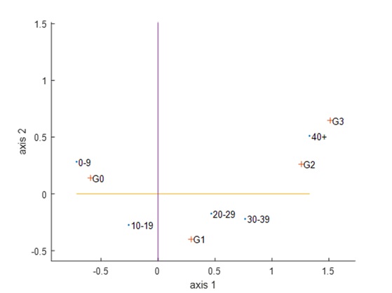
Figure 1: CA map of asbestos exposure data.

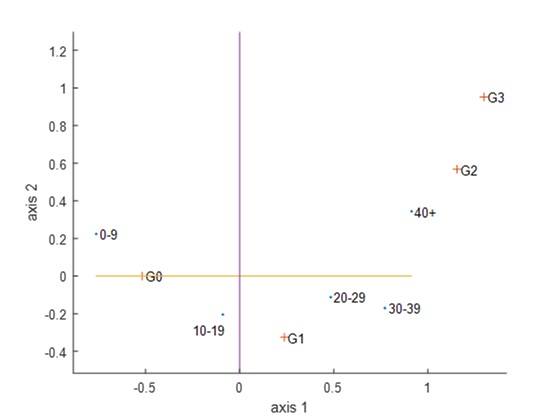
Figure 2: TCA map of asbestos exposure data.

3.2 Western Hemisphere countries and their memberships in trade and treaty organizations

Table 4 presents a two-mode affiliation network matrix ${\mathbf{Z}}=(z_{ij})$ of size $22\times 15$ taken from Faust (2005). The 22 rows represent 22 countries and the 15 columns the regional trade and treaty organizations, described in Appendix A. The country $i$ is a member of the organization $j$ if $z_{ij}=1$; and $z_{ij}=0$ means the country $i$ is not a member of the organization $j$. Faust (2005) visualized this data by correspondence analysis, see Figure 3, which is quite cluttered. She interpreted the first two principal dimensions by examining the factor scores of the countries and summarized the results in 3 points:

a) The first dimension contrasts South American countries and organizations on the one hand, and Central American countries and organizations on the other hand.

b) The second dimension clearly distinguishes Canada and the United States (both North American countries) along with NAFTA from other countries and organizations. In CA, the relative contribution of Canada (resp. US) to the second axis is $RC_{2}^{CA}(Canada)=RC_{2}^{CA}(US)=0.409$, and $RC_{2}^{CA}(NAFTA)=0.821.$

c) Organizations (SELA, OAS, and IDB) are in the center because they have membership profiles that are similar to the marginal profile: almost all countries belong to (SELA, OAS, and IDB), see Table 4.

Figure 4 provides the TCA map, which is much more interpretable than the corresponding CA map in Figure 3; where we see that, additionally to the three points mentioned by Faust (2005), the south american countries are divided into two groups, northern (Venezuela, Bolivia, Peru and Ecuador) and southern countries (Brazil, Uruguay, Argentina, Paraguay and Chile). Furthermore, the contributions of the points Canada, the United States, and NAFTA to the second axis are not substantial compared to CA: $RC_{2}^{TCA}(Canada)=RC_{2}^{TCA}(US)=0.088$, and $RC_{2}^{TCA}(NAFTA)=0.10.$ This shows the robustness of TCA due to the robustness of the $\delta$ statistic.

It is well known that, CA is very sensitive to some particularities of a data set; further, how to identify and handle these is an open unresolved problem. However, for contingency tables Choulakian (2017) enumerated three under the umbrella of sparse contingency tables: rare observations, zero-block structure and relatively high-valued cells. It is evident that this data set has specially three rare observations (NAFTA, CANADA and USA), which determine the 2nd dimension of CA. A row or a column is considered rare, if its marginal probablity is quite small.

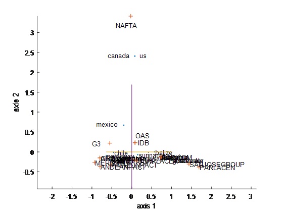
Figure 3: CA map of Western Hemisphere affinity network.

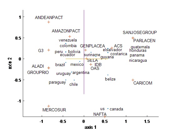
Figure 4: TCA map of Western Hemisphere affinity network.

Table 4: Sociomatrix of American countries and their memberships.
Countries	Regional Trade and Treaty Organizations
	1	2	3	4	5	6	7	8	9	10	11	12	13	14	15	Sum
Argentina	0	1	0	0	0	1	1	0	1	1	0	1	0	0	1	7
Belize	1	0	0	0	1	0	0	0	1	0	0	1	0	0	1	5
Bolivia	0	1	1	1	0	1	1	0	1	0	0	1	0	0	1	8
Brazil	0	1	1	0	0	1	1	0	1	1	0	1	0	0	1	8
Canada	0	0	0	0	0	0	0	0	1	0	1	1	0	0	0	3
Chile	0	1	0	0	0	0	1	0	1	0	0	1	0	0	1	5
Colombia	1	1	1	1	0	1	1	1	1	0	0	1	0	0	1	10
CostaRica	1	0	0	0	0	1	0	0	1	0	0	1	0	1	1	6
Ecuador	0	1	1	1	0	1	1	0	1	0	0	1	0	0	1	8
ElSalvador	1	0	0	0	0	1	0	0	1	0	0	1	1	1	1	7
Guatemala	1	0	0	0	0	1	0	0	1	0	0	1	1	1	1	7
Guyana	1	0	1	0	1	1	0	0	1	0	0	1	0	0	1	7
Honduras	1	0	0	0	0	1	0	0	1	0	0	1	1	1	1	7
Mexica	1	1	0	0	0	1	1	1	1	0	1	1	0	0	1	9
Nicaragua	1	0	0	0	0	1	0	0	1	0	0	1	0	1	1	6
Panama	1	0	0	0	0	1	0	0	1	0	0	1	0	1	1	6
Paraguay	0	1	0	0	0	0	1	0	1	1	0	1	0	0	1	6
Peru	0	1	1	1	0	1	1	0	1	0	0	1	0	0	1	8
Suriname	1	0	1	0	0	0	0	0	1	0	0	1	0	0	1	5
UnitedStates	0	0	0	0	0	0	0	0	1	0	1	1	0	0	0	3
Uruguay	0	1	0	0	0	1	1	0	1	1	0	1	0	0	1	7
Venezuela	1	1	1	1	0	1	1	1	1	0	0	1	0	0	1	10
Sum	12	11	8	5	2	16	11	3	22	5	3	22	3	6	20	149

3.3 Maximal interaction two-mode clustering of continuous data

Schepers, Bock and Van Mechelen (2017) discussed maximum interaction two-mode clustering of continuous data. By generalizing their objective function, we want to show that the results of this section can be considered a particular robust L${}_{1}\$variant of their approach. Let ${\mathbf{Y}=(}y_{ij})\$be a 2-way array for $i\in I,$ $j\in J$. As usual, we define, for instance, $\overline{y}_{\ast j}=\sum_{i=1}^{n}\frac{y_{ij}}{n}$ and $\overline{y}_{\ast\ast}=\sum_{j=1}^{m}\sum_{i=1}^{n}\frac{y_{ij}}{mn}.$ Let ${\mathbf{X}=(}x_{ij})$ be the additive double-centered array, where

$$x_{ij}=y_{ij}-\overline{y}_{i\ast}-\overline{y}_{\ast j}+\overline{y}_{\ast\ast}.$$

In the jargon of statistics, the cell $x_{ij}$ represents the additive 2-way interaction of the cell ($i,j)\in I\times J.$ The matrix ${\mathbf{X}}$ is double-centered, and it satisfies equations (6) through (10). Let $I=U_{\alpha=1}^{r}S_{\alpha}$ be an $r$-partition of $I$ and $J=U_{\beta=1}^{c}T_{\beta}$ be a $c$-partition of $J.$ We consider the following maximization of the overall interaction problem for $p\geq 1$

$$f_{p}(S_{\alpha},T_{\beta}:\alpha=1,...,r\ \text{and}\ \beta=1,...,c)=\sum_{\alpha=1}^{r}\sum_{\beta=1}^{c}|S_{\alpha}|\ |T_{\beta}|\ g_{p}(\alpha,\beta),$$

where $|S_{\alpha}|$ is the cardinality of the set $S_{\alpha}$ and

$$g_{p}(\alpha,\beta)=\left(|\frac{\sum_{i\in S_{\alpha}}\sum_{j\in T_{\beta}}x_{ij}}{|S_{\alpha}|\ |T_{\beta}|\ }|\right)^{p}.$$

When $p=2$, then maximizing $f_{2}(S_{\alpha},T_{\beta}:\alpha=1,...,r\$and$\ \beta=1,...,c),$ named maximal overall interaction, is the criterion computed in Schepers et. al (2017). When $p=1,\ r=c=2,$ then maximizing $f_{1}(S_{\alpha},T_{\beta}:\alpha=1,...,2\$and$\ \beta=1,...,2)=||{\mathbf{X}||}_{\infty\rightarrow 1}=4||{\mathbf{X}||}_{\boxdot}$ by Lemma 3, which is the criterion computed in TCA.

4 Triple-centered arrays

To motivate our subject, we start with an example. Let ${\mathbf{Y}=(}y_{ijk})\$be a 3-way array for $i\in I,$ $j\in J$ and $k\in K=\left\{1,2,...,t\right\}.$ As usual, we define, for instance, $\overline{y}_{ij\ast}=\sum_{k=1}^{t}y_{ijk}/t,,$ $\overline{y}_{\ast j\ast}=\sum_{k=1}^{t}\sum_{i=1}^{n}\frac{y_{ijk}}{tn}$ and $\overline{y}_{\ast\ast\ast}=\sum_{k=1}^{t}\sum_{j=1}^{m}\sum_{i=1}^{n}\frac{y_{ijk}}{tmn}.$ Let ${\mathbf{X}=(}x_{ijk})$ be the triple-centered array, where

$$x_{ijk}=y_{ijk}-\overline{y}_{ij\ast}-\overline{y}_{i\ast k}-\overline{y}_{\ast jk}+\overline{y}_{i\ast\ast}+\overline{y}_{\ast j\ast}+\overline{y}_{\ast\ast k}-\overline{y}_{\ast\ast\ast}.$$

In the jargon of statistics, the cell $x_{ijk}$ represents the additive 3-way interaction of the cell ($i,j,k)\in I\times J\times K.$ The tensor ${\mathbf{X}}$ is triple-centered; that is,

$$\sum_{k=1}^{t}x_{ijk}=\sum_{j=1}^{n}x_{ijk}=\sum_{i=1}^{m}x_{ijk}=0.$$

A generalization of Lemma 3 is

Lemma 4: (8-equal parts property) The tensor norm

$$||{\mathbf{X}}||_{(\infty,\infty)\rightarrow 1} = \max\sum_{k\in K}\sum_{j\in J}\sum_{i\in I}w_{k}v_{j}u_{i}x_{ijk}\ \text{subject to}\ {\mathbf{u}\times v}\times{\mathbf{w}}\in\left\{-1,+1\right\}^{m\times n\times t}$$

$$= 8\sum_{k\in W_{opt}}\sum_{j\in T_{opt}}\sum_{i\in S_{opt}}x_{ijk}\geq 8\sum_{k\in W}\sum_{j\in T}\sum_{i\in S}x_{ijk},$$

where $W\subset K.$

The proof is similar to the proof of Lemma 3.

Lemma 4 can easily be generalized to higher-way arrays.

4.1 Conclusion

This essay is an attempt to emphasize the following two points.

First, we showed the optimality and robustness of the mean absolute deviations about the mean, its interpretation, and its generalization to higher-way arrays. A key notion in describing its robustness is that the relative contribution of a point is bounded by 50%.

Second, within the framework of TCA, we showed that the following three identities $\delta_{1}=||{\mathbf{P}}_{1}||_{\infty\rightarrow 1}=4||{\mathbf{P}}_{1}{\mathbf{|}|}_{\boxdot}$ reveal three different but related aspects of TCA: a) $\delta_{1}$, computed in (17) and (18), represents the mean of absolute deviations about the mean statistic; b) The taxicab norm $||{\mathbf{P}}_{1}||_{\infty\rightarrow 1},$ via (15) and (16), shows that uniform weights are affected to the columns and the rows; c) The cut norm $4||{\mathbf{P}}_{1}{\mathbf{|}|}_{\boxdot}$ shows that the computation of each principal dimension of TCA corresponds to balanced 2-blocks seriation, with equality of the cut norm in the 4 associated blocks.

Acknowledgements.

Choulakian’s research has been supported by NSERC grant (RGPIN-2017-05092) of Canada. The authors thank William Alexander Digout for help in computations.

5 References

Beh, E. and Lombardo, R. (2014). Correspondence Analysis: Theory, Practice and New Strategies. N.Y: Wiley.

Benzécri, J.P. (1973). L’Analyse des Données: Vol. 2: L’Analyse des Correspondances. Paris: Dunod.

Benzécri, J.P (1992). Correspondence Analysis Handbook. N.Y: Marcel Dekker.

Choulakian, V. (2006). Taxicab correspondence analysis. Psychometrika, 71, 333-345

Choulakian, V. (2008a). Taxicab correspondence analysis of contingency tables with one heavyweight column. Psychometrika, 73, 309-319.

Choulakian, V. (2008b). Multiple taxicab correspondence analysis. Advances in Data Analysis and Classification, 2, 177-206.

Choulakian, V. and de Tibeiro, J. (2013a). Graph partitioning by correspondence analysis and taxicab correspondence analysis. Journal of Classification, 30, 397-427.

Choulakian, V., Allard, J. and Simonetti, B. (2013b). Multiple taxicab correspondence analysis of a survey related to health services. Journal of Data Science, 11(2), 205-229.

Choulakian, V., Simonetti, B. and Gia, T.P. (2014). Some further aspects of taxicab correspondence analysis. Statistical Methods and Applications, available online.

Choulakian, V. (2016). Matrix factorizations based on induced norms. Statistics, Optimization and Information Computing, 4, 1-14.

Choulakian, V. (2017). Taxicab correspondence analysis of sparse two-way contingency tables. Statistica Applicata - Italian Journal of Applied Statistics, 29 (2-3), 153-179.

Faust, K. (2005). Using correspondence analysis for joint displays of affiliation networks. In: Carrington, P.J., Scott, J., Wasserman, S. (Eds.), Models and Methods in Social Network Analysis. Cambridge University Press, Cambridge, 117–147.

Gifi, A. (1990). Nonlinear Multivariate Analysis. N.Y:  Wiley.

Gorard, S. (2015). Introducing the mean absolute deviation ‘effect’ size. International Journal of Research & Method in Education, 38 (2), 105–114.

Greenacre, M. (1984). Theory and Applications of Correspondence Analysis. Academic Press, London.

Jensen, S.T. (1999). The Laguerre-Samuelson inequality with extensions and applications in Statistics and Matrix Theory. MS thesis, McGill University.

Khot, S. and Naor, A. (2012). Grothendieck-type inequalities in combinatorial optimization. Communications on Pure and Applied Mathematics, Vol. LXV, 992–1035.

Le Roux, B. and Rouanet, H. (2004). Geometric Data Analysis. From Correspondence Analysis to Structured Data Analysis. Dordrecht: Kluwer–Springer.

Liiv, I. (2010). Seriation and matrix reordering methods: An historical overview. Statistical Analysis and Data Mining, 3(2), $70-91$.

Murtagh, F. (2005). Correspondence Analysis and Data Coding with Java and R. Boca Raton, FL., Chapman & Hall/CRC.

Nishisato, S. (1984). Forced classification: A simple application of a quantification method. Psychometrika, 49(1), 25-36.

Nishisato, S. (2007). Mutidimensional nonlinear descriptive analysis. Chapman & Hall/CRC, Boca Raton.

Pham-Gia, T. and Hung, T.L. (2001). The mean and median absolute deviations. Mathematical and Computer Modelling, 34, 921-936.

Schepers, J., Bock, H-H. and Van Mechelen, I. (2017). Maximal interaction two-mode clustering. Journal of Classification, 34, 49-75.

Yitzhaki, S. and Lambert, P.J. (2013). The relationship between the absolute deviation from a quantile and Gini’s mean difference. Metron, 71, 97–104

Appendix A: List of Western Hemisphere Organizations

1.  Association of Caribbean States (ACS): Trade group sponsored by the Caribbean Commnnity and Common Market (CARlCOM).

2.  Latin American Integration Association (ALADI): Free trade organization.

3.  Amazon Pact: Promotes development of Amazonian territories.

4.  Andean Pact: Promotes development of members through economic and social integration.

5.  Caribbean Commnnity and Common Market (CARICOM): Caribbean trade organization; promotes economic development of members.

6.  Group of Latin American and Caribbean Sugar Exporting Countries (GEPLACEA): Sugar-producing and exporting countries.

7.  Group of Rio: Organization for joint political action.

8.  Group of Three (G-3): Trade organization.

9.  Inter-American Development Bank (IDB): Promotes development of member nations.

10.  South American Common Market (MERCOSUR): Increases economic cooperation in the region.

11.  North American Free Trade Agreement (NAFTA): Free trade organization.

12.  Organization of American States (OAS): Promotes peace, security, economic, and social development in the Western Hemisphere.

13.  Central American Parliament (PARLACÉN): Works for the political integration of Central America.

14.  San José Group: Promotes regional economic integration.

15.  Latin American Economie System (SELA): Promotes economic and social development of member nations.