Voter and Majority Dynamics with Biased and Stubborn Agents

Abstract

We study binary opinion dynamics in a fully connected network of interacting agents. The agents are assumed to interact according to one of the following rules: (1) Voter rule: An updating agent simply copies the opinion of another randomly sampled agent; (2) Majority rule: An updating agent samples multiple agents and adopts the majority opinion in the selected group. We focus on the scenario where the agents are biased towards one of the opinions called the preferred opinion. Using suitably constructed branching processes, we show that under both rules the mean time to reach consensus is $\Theta(\log N)$, where $N$ is the number of agents in the network. Furthermore, under the majority rule model, we show that consensus can be achieved on the preferred opinion with high probability even if it is initially the opinion of the minority. We also study the majority rule model when stubborn agents with fixed opinions are present. We find that the stationary distribution of opinions in the network in the large system limit using mean field techniques.

1 Introduction

The problem of social learning Ellison_JPE_1993 ; Chatterjee_AAP_2004 is concerned with the rate at which social agents, interacting under simple rules, can learn/discover the true utilities of their choices, opinions or technologies. In this context, the two central questions we study are: (1) Can social agents learn/adopt the better technology/opinion through simple rules of interactions and if so, how fast? and (2) What are the effects of the presence of stubborn agents (having fixed opinions) on the dynamics opinion diffusion?

We consider a setting where the choices available to each agent are binary and are represented by $\left\{{0}\right\}$ and $\left\{{1}\right\}$ Chatterjee_AAP_2004 ; Bandyopadhyay_EJP_2010 . These are referred to as opinions of the agents. The interactions among the agents are modelled using two simple rules: the voter rule Ligett_voter_model ; Sudbury_voter_model ; Cox_voter_model and the majority rule Krapivsky_majority ; Redner_majority ; Chen_majority ; ganesh_consensus . In the voter rule, an agent randomly samples one of its neighbours at an instant when it decides to update its opinion. The updating agent then adopts the opinion of the sampled neighbour. This simple rule captures the tendency of an individual to mimic other individuals in the society. In the majority rule, instead of sampling a single agent, an updating agent samples $2K$ ($K\geq 1$) neighbours and adopts the opinion of the majority of the sampled neighbours (including itself). This rule captures the tendency of the individuals to conform with the majority opinion in their local neighbourhoods.

Related literature: The voter model and its variants have been studied extensively (see emanuele_review for a recent survey) for different network topologies, e.g., finite integer lattices in different dimensions  Cox_voter_model ; Krapivsky_voter , complete graphs with three states three_state_voter_vojnovic , heterogeneous graphs Redner_voter , random $d$-regular graphs cooper_voter , Erdos-Renyi random graphs, and random geometric graphs Yildiz_ITA etc. It is known peleg_voter ; nakata_voter that if the underlying graph is connected, then the classical voter rule leads to a consensus where all agents adopt the same opinion. Furthermore, if $A$ is the set of all agents having an opinion $i\in\left\{{0,1}\right\}$ initially, then the probability that consensus is achieved on opinion $i$ (referred to as the exit probability to opinion $i$) is given by $d(A)/2m$, where $d(A)$ is the sum of the degrees of the vertices in $A$ and $m$ is the total number of edges in the graph. It is also known that for most network topologies the mean consensus time is $\Omega(N)$, where $N$ is the total number of agents. In Mobilia_voter_stubborn ; Yildiz_voter_stubborn , the voter model was studied under the presence of stubborn individuals who do not update their opinions. In such a scenario, the network cannot reach a consensus because of the presence of stubborn agents having both opinions. Using coalescing random walk techniques the average opinion in the network and the variance of opinions were computed at steady state.

The majority rule model was first studied in Galam_majority , where it was assumed that, at every iteration, groups of random sizes are formed by the agents. Within each group, the majority opinion is adopted by all the agents. Similar models with fixed (odd) group size have been considered in Krapivsky_majority ; Redner_majority . A more general majority rule based model is analysed in ganesh_consensus for complete graphs. It has been shown that with high probability (probability tending to one as $N\to\infty$) consensus is achieved on the opinion with the initial majority and the mean time to reach consensus time is $\Theta(\log N)$. The majority rule model is studied for random $d$-regular graphs on $N$ vertices in majority_regular_collin . It is shown that when the initial imbalance of between the two opinions is above $c\sqrt{1/d+d/N}$, for some constant $c>0$, then consensus is achieved in $O(\log N)$ time on the initial majority opinion with high probability. A deterministic version of the majority rule model, where an agent, instead of randomly sampling some of its neighbours, adopts the majority opinion among all its neighbours, is considered in Mossel_majority_new ; Flocchini_majority_new ; Moran_majority_new ; AGUR1_majority . In such models, given the graph structure of the network, the opinions of the agents at any time is a deterministic function of the initial opinions of the agents. The interest there is to find out the initial distribution of opinions for which the network converges to some specific absorbing state.

Contributions: In all the prior works on the voter and the majority rule models, it is assumed that opinions or technologies are indistinguishable. However, in a social learning model, one opinion/technology may be inherently ‘better’ than the other leading to more utility to individuals choosing the better option in a round of update. As a result, individuals currently using the better technology will update less frequently than individuals with the worse technology. To model this scenario, we assume that an agent having opinion $i\in\left\{{0,1}\right\}$ performs an update with probability $q_{i}$. By choosing $q_{1}<q_{0}$, we make the agents ‘biased’ towards the opinion $\left\{{1}\right\}$, which is referred to as the preferred opinion. We study the opinion dynamics under both voter and majority rules when the agents are biased. We focus on the case where the underlying graph is complete which closely models situations where agents are mobile and can therefore sample any other agent depending on their current neighbourhood.

For the voter model with biased agents, we show that the probability of reaching consensus on the non-preferred opinion decreases exponentially with the network size. Furthermore, the mean consensus time is shown to be logarithmic in the network size. This is in sharp contrast to the voter model with unbiased agents where the probability of reaching consensus on any opinion remains constant and the mean consensus time grows linearly with the network size. Therefore, in the biased voter model consensus is achieved exponentially faster than that in the unbiased voter model.

For the majority rule model with biased agents, we show that the network reaches consensus on the preferred opinion with high probability only if the initial fraction of agents with the preferred opinion is above a certain threshold determined by the biases of the agents. Furthermore, as in the voter model, the mean consensus time is shown to be logarithmic in the network size. Our results generalise existing results on the majority rule model with unbiased agents where it is known that consensus is achieved (with high probability) on the opinion with the initial majority and the mean consensus time is logarithmic in the network size. However, existing proofs for the unbiased majority rule model Krapivsky_majority ; ganesh_consensus cannot be extended to the biased case as they crucially rely on the fact that opinions are indistinguishable. We use suitably constructed branching processes and monotonicity of certain rational polynomials to prove the results for the biased model.

We also study the majority rule model in the presence of agents having fixed opinions at all times. These agents are referred to as ’stubborn’ agents. A similar study of the voter model in the presence of stubborn agents was done in Yildiz_voter_stubborn . In presence of stubborn agents, the network cannot reach a consensus state. The key objective, therefore, is to study the stationary distribution of opinions among the non-stubborn agents. In Yildiz_voter_stubborn , coalescing random random walk techniques were used to study this stationary distribution of opinions. However, such techniques do not apply to majority rule dynamics. We analyse the network dynamics in the large scale limit using mean field techniques. In particular, we show that depending on the proportions of stubborn agents the mean field can either have single or multiple equilibrium points. If multiple equilibrium points are present, the network shows metastability in which it switches between stable configurations spending long time in each configuration.

An earlier version of this work arpan_opinion_ITC , contained some of the results of this paper and an analysis of the majority rule model for $K=1$. However, only sketches of the proofs were provided. In the current paper, we provide rigorous proofs of all results and a more general analysis of the majority rule model (for $K\geq 1$).

Organisation: The rest of the paper is organised as follows. In Section 2, we introduce the model with biased agents. In Sections 3 and 4, we state the main results for the voter model and the majority rule model with biased agents, respectively. Section 5 analyses the majority rule model with stubborn agents. In Sections 6-10, we provide the detailed proofs the main results on voter and majority rule models with biased agents. Finally, the paper is concluded in Section 11.

2 Model with biased agents

We consider a network of $N$ social agents. Opinion of each agent is assumed to be a binary variable taking values in the set $\{0,1\}$. Initially, every agent adopts one of the two opinions. Each agent considers updating its opinion at points of an independent unit rate Poisson point process associated with itself. At a point of the Poisson process associated with itself, an agent either updates its opinion or retains its past opinion. We assume that an agent with opinion $i\in\left\{{0,1}\right\}$ updates its opinion at a point of the unit rate Poisson process associated with itself with probability $q_{i}\in(0,1)$ and retains its opinion with probability $p_{i}=1-q_{i}$. To make the agents ‘biased’ towards opinion $\left\{{1}\right\}$ we assume that $q_{0}>q_{1}$ which implies that an agent with opinion $\left\{{1}\right\}$ updates its opinion less frequently than an agent with opinion $\left\{{0}\right\}$.

In case the agent decides to update its opinion, it does so either using the voter rule or under the majority rule. In the voter rule, an updating agent samples an agent uniformly at random from $N$ agents (with replacement) from the network and adopts the opinion of the sampled agent. In the majority rule, an updating agent samples $2K$ agents ($K\geq 1$) uniformly at random (with replacement) and adopts the opinion of the majority of the $2K+1$ agents including itself. The results derived in this paper can be extended to the case where the updating agent samples an agent from a random group of size $O(N)$. However, for simplicity we only focus on the case where sampling occurs from the whole population.

3 Main results for the voter model with biased agents

We first consider the voter model with biased agents. In this case, clearly, the network reaches consensus in a finite time with probability 1. Our interest is to find out the probability with which consensus is achieved on the preferred opinion $\{1\}$. This is referred to as the exit probability of the network. We also intend to characterise the average time to reach the consensus.

The case $q_{1}=q_{0}=1$ is referred to as the voter model with unbiased agents, which has been analysed in Ligett_voter_model ; Sudbury_voter_model . It is known that for unbiased agents the probability with which consensus is reached on a particular opinion is simply equal to the initial fraction $\alpha$ of agents having that opinion and the expected time to reach consensus for large $N$ is approximately given by $Nh(\alpha)$, where $h(\alpha)=-[\alpha\ln(\alpha)+(1-\alpha)\ln(1-\alpha)]$. We now proceed to characterise these quantities for the voter model with biased agents.

Let $X^{(N)}(t)$ denote the number of agents with opinion $\{1\}$ at time $t\geq 0$. Clearly, $X^{(N)}(\cdot)$ is a Markov process on state space $\{0,1,\ldots,N\}$, with absorbing states $0$ and $N$. The transition rates from state $k$ are given by

$$q(k\to k+1) =q_{0}k\frac{N-k}{N},$$ (1)

$$q(k\to k-1) =q_{1}k\frac{N-k}{N},$$ (2)

where $q(i\to j)$ denotes the rate of transition from state $i$ to state $j$. The embedded discrete-time Markov chain $\tilde{X}^{(N)}$ for $X^{(N)}$ is a one-dimensional random walk on $\left\{{0,1,\ldots,N}\right\}$ with jump probability of $p=q_{0}/(q_{0}+q_{1})$ to the right and $q=1-p$ to the left. We define $r=q/p<1$ and $\bar{r}=1/r$. Let $T_{k}$ denote the first hitting time of state $k$, i.e.,

$$T_{k}=\inf\left\{{t\geq 0:X^{(N)}(t)\geq k}\right\},$$ (3)

We are interested in the asymptotic behaviour of the quantities $E_{N}(\alpha):=\mathbb{P}_{\left\lfloor{\alpha N}\right\rfloor}\left({T_{N}<T_{0}}\right)$ and $t_{N}(\alpha)=\mathbb{E}_{{\left\lfloor{\alpha N}\right\rfloor}}\left[{T_{0}\wedge T_{N}}\right]$, where $\mathbb{P}_{x}\left({\cdot}\right)$ and $\mathbb{E}_{x}\left[{\cdot}\right]$, respectively denote the probability measure and expectation conditioned on the event $X^{(N)}(0)=x$. To characterise the above quantities we require the following lemma which follows from the gambler ruin identity for one-dimensional asymmetric random walks Spitzer_book .

Lemma 1

For $0\leq a<x<b\leq N$, we have

$$\mathbb{P}_{x}\left({T_{a}<T_{b}}\right)=\frac{r^{x}-r^{b}}{r^{a}-r^{b}}.$$ (4)

From the above lemma it follows that

$$E_{N}(\alpha) =\mathbb{P}_{\left\lfloor{\alpha N}\right\rfloor}\left({T_{N}<T_{0}}\right),$$

$$=\frac{1-r^{\left\lfloor{\alpha N}\right\rfloor}}{1-r^{N}},$$

$$\geq 1-r^{\left\lfloor{\alpha N}\right\rfloor}=1-\exp(-cN),$$

for some constant $c>0$ (since $r<1$). Hence, the probability of having a consensus on the non-preferred opinion approaches $0$ exponentially fast in $N$. This is unlike the voter model with unbiased agents where the probability of having consensus on either opinion remains constant with respect to $N$.

The following theorem characterises the mean time ${t}_{N}(\alpha)$ to reach the consensus state starting from $\alpha$ fraction of agents having opinion $\{1\}$.

Theorem 3.1

For all $\alpha\in(0,1)$ we have $t_{N}(\alpha)=\Theta(\log N)$.

Hence, the above theorem shows that the mean consensus time in the biased voter model is logarithmic in the network size. This is in contrast to the voter model with unbiased agents where the mean consensus time is linear in the network size. Thus, with biased agents, the network reaches consensus exponentially faster.

We now consider the measure-valued process $x^{(N)}=X^{(N)}/N$, which describes the evolution of the fraction of agents with opinion $\{1\}$. We show that the following convergence takes place.

Theorem 3.2

If $x^{(N)}(0)\Rightarrow\alpha$, then $x^{(N)}(\cdot)\Rightarrow x(\cdot)$, where $\Rightarrow$ denotes weak convergence and $x(\cdot)$ is a deterministic process with initial condition $x(0)=\alpha$ and is governed by the following differential equation

$$\dot{x}(t)=(q_{0}-q_{1})x(t)(1-x(t)),$$ (5)

According to the above result, for large $N$, the process $x^{(N)}(\cdot)$ is well approximated by the deterministic process $x(\cdot)$ which is generally referred to as the mean field limit of the system. Using the mean field limit, we can approximate the mean consensus time $t_{N}(\alpha)$ by the time the process $x(\cdot)$ takes to reach the state $1-1/N$ starting from $\alpha$.

Theorem 3.3

1. For the process $x(\cdot)$ defined by (5), we have $x(t){\to}1$ as $t\to\infty$ for any $x(0)\in(0,1)$.

2. Let $t(\epsilon,\alpha)$ denote the time required by the process $x(\cdot)$ to reach $\epsilon\in(0,1)$ starting from $x(0)=\alpha\in(0,1)$. Then

   $$t(\epsilon,\alpha)=\frac{1}{q_{0}-q_{1}}\left({\log\frac{\epsilon}{1-\epsilon}-\ln\frac{\alpha}{1-\alpha}}\right).$$ (6)

   In particular, for $\epsilon=1-1/N$ we have

   $$t(1-1/N,\alpha) =\frac{1}{q_{0}-q_{1}}\log(N-1)-\frac{1}{q_{0}-q_{1}}\log\left({\frac{\alpha}{1-\alpha}}\right).$$ (7)

Proof

Since $q_{0}>q_{1}$ and $x(t)\in(0,1)$ for all $t\geq 0$, we have from (5) that $\dot{x}(t)\geq 0$ for all $t\geq 0$. Hence, $x(t)\to 1$ as $t\to\infty$.

The second assertion follows directly by solving (5) with initial condition $x(0)=\alpha$. ∎

Remark 1

It is worth noting here that the process $x(\cdot)$ does not reach $1$ in a finite time even though the process $x^{(N)}(\cdot)$ does reach $1$ in a finite time with probability $1$. However, it is ‘reasonable’ to assume that $t_{N}(\alpha)$ is ’closely’ approximated by $t(1-1/N,\alpha)$. Such approximation of the absorption time of an absorbing Markov chain using its corresponding mean field limit is common in the literature three_state_voter_vojnovic ; Krapivsky_majority . However, except from a few special cases, e.g. gast_absorption , there is no general theory justifying such approximations.

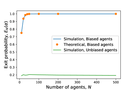
Figure 1: Exit probability $E_{N}(\alpha)$ as a function of the number of agents $N$. Parameters: $q_{0}=1$, $q_{1}=0.5$, $\alpha=0.2$.

Simulation Results: In Figure 1, we plot the exit probability for both unbiased ($q_{0}=q_{1}=1$) and biased ($1=q_{0}>q_{1}=0.5$) cases as functions of the number of agents $N$ for $\alpha=0.2$. As expected from our theory, we observe that in the biased case the exit probability exponentially increases to $1$ with the increase $N$. This is in contrast to the unbiased case, where the exit probability remains constant at $\alpha$ for all $N$.

In Figure 2(a), we plot the mean consensus time ${t}_{N}(\alpha)$ for both unbiased and biased cases as a function of $N$ for $\alpha=0.4$. We observe a good match between the estimate obtained in Theorem 3.3 and the simulation results. The observation also verifies the statement of Theorem 3.1. In Figure 2(b), we plot the mean consensus time as a function of $\alpha$ for both biased an unbiased cases. The network size is kept fixed at $N=100$. We observe that for the unbiased case, the consensus time increases in the range $\alpha\in(0,0.5)$ and decreases in the range $\alpha\in(0.5,1)$. In contrast, for the biased case, the consensus time steadily decreases with the increase in $\alpha$. This is expected since, in the unbiased case, consensus is achieved faster on a particular opinion if the initial number agents having that opinion is more than the initial number of agents having the other opinion. On the other hand, in the biased case, consensus is achieved with high probability on the preferred opinion and therefore increasing the initial fraction of agents having the preferred opinion always decreases the mean consensus time.

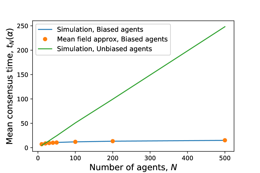
(a) Mean consensus time ${t}_{N}(\alpha)$ as a function of the number of agents $N$

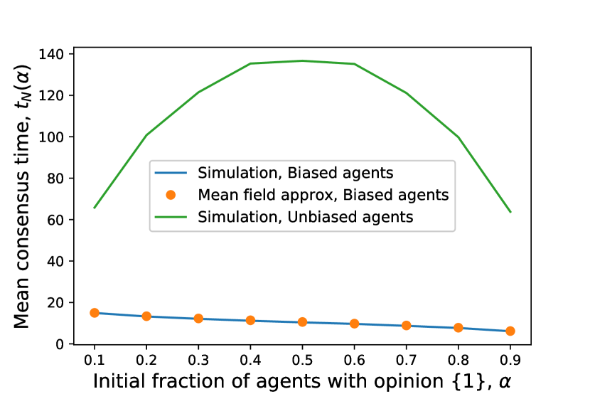
(b) Mean consensus time ${t}_{N}(\alpha)$ as a function of the initial fraction $\alpha$ of agents with opinion $\{1\}$.

Figure 2: Mean consensus time under the voter model with biased agents

4 Main results for the majority rule model with biased agents

In this section, we consider the majority rule model with biased agents. As in the voter model, it is easy to see that in this case a consensus is achieved in a finite time with probability 1. We proceed to find the exit probability to opinion ${1}$ and the mean consensus time.

Let $X^{(N)}(t)$ denote the number of agents with opinion $\{1\}$ at time $t\geq 0$. Clearly, $X^{(N)}(\cdot)$ is a Markov process on state space $\{0,1,\ldots,N\}$. The jump rates of $X^{(N)}$ from state $n$ to state $n+1$ and $n-1$ are given by

$$q(n\to n+1) =(N-n)q_{0}\sum_{i=K+1}^{2K}\binom{2K}{i}\left({\frac{n}{N}}\right)^{i}\left({\frac{N-n}{N}}\right)^{2K-i},$$ (8)

$$=(N-n)q_{0}\mathbb{P}\left({\text{Bin}\left({2K,\frac{n}{N}}\right)\geq K+1}\right),$$ (9)

$$q(n\to n-1) =nq_{1}\sum_{i=K+1}^{2K}\binom{2K}{i}\left({\frac{N-n}{N}}\right)^{i}\left({\frac{n}{N}}\right)^{2K-i},$$ (10)

$$=nq_{1}\mathbb{P}\left({\text{Bin}\left({2K,1-\frac{n}{N}}\right)\geq K+1}\right),$$ (11)

respectively. Let $\tilde{X}^{(N)}$ denote the embedded Markov chain corresponding to $X^{(N)}$. Then the jump probabilities for the embedded chain $\tilde{X}^{(N)}$ are given by

$$p_{n,n+1} =1-p_{n,n-1}$$

$$=\frac{q(n\to n+1)}{q(n\to n-1)+q(n\to n+1)}$$

$$=\frac{g_{K}(n/N)}{g_{K}(n/N)+r},$$ (12)

where $1\leq n\leq N-1$, $r=q_{1}/q_{0}<1$, and $g_{K}:(0,1)\to(0,\infty)$ is defined as

$$g_{K}(x)=\frac{\frac{1}{x}\mathbb{P}\left({\text{Bin}(2K,x)\geq K+1}\right)}{\frac{1}{1-x}\mathbb{P}\left({\text{Bin}\left({2K,1-x}\right)\geq K+1}\right)}.$$ (13)

With probability $1$, $X^{(N)}$ gets absorbed in one of the states $0$ or $N$ in finite time. We are interested in the probability of absorption in the state $N$ and the average time till absorption. We first state the following lemma which is key to proving many of the results in this section.

Lemma 2

The function $g_{K}:(0,1)\to(0,\infty)$ as defined by (13) is strictly increasing and is therefore also one-to-one.

In the following theorem, we characterise the exit probability to state $N$.

Theorem 4.1

1. Let $E_{N}(n)$ denote the probability that the process $X^{(N)}$ gets absorbed in state $N$ starting from state $n$. Then, we have

   $$E_{N}(n)=\frac{\sum_{t=0}^{{n}-1}\prod_{j=1}^{t}\frac{r}{g_{K}(j/N)}}{\sum_{t=0}^{N-1}\prod_{j=1}^{t}\frac{r}{g_{K}(j/N)}},$$ (14)

2. Define $E_{N}(\alpha):=E_{N}(\left\lfloor{\alpha N}\right\rfloor)$ and $\beta:=g_{K}^{-1}(r)$. Then $E_{N}(\alpha)\to 1$ (resp. $E_{N}(\alpha)\to 0$) as $N\to\infty$ if $\alpha>\beta$ (resp. $\alpha<\beta$) and this convergence is exponential in $N$.

Hence, a phase transition of the exit probability occurs at $\beta=g_{K}^{-1}\left({r}\right)$ for all values of $K\geq 1$. This implies, that even though the agents are biased towards the preferred opinion, consensus may not be obtained on the preferred opinion if the initial fraction of agents having the preferred opinion is below the threshold $\beta$. This is in contrast to the voter model, where consensus is obtained on the preferred opinion irrespective of the initial state. The threshold $\beta$ can be computed by solving $g_{K}(\beta)=r$ using either Newton-Raphson method or other fixed point methods.

Remark 2

We note that for the unbiased majority rule model we have $r=1$ and $\beta=g_{K}^{-1}(r)=g_{K}^{-1}(1)=1/2$. Thus, the known results ganesh_consensus ; Krapivsky_majority for the majority rule model with unbiased agents are recovered.

We now characterise the mean time ${t}_{N}(\alpha)$ to reach the consensus state starting from $\alpha$ fraction of agents having opinion $\{1\}$. As before, we define $T_{n}$ to be the random time of first hitting the state $n$, i.e., $T_{n}=\inf\left\{{t\geq 0:X^{(N)}(t)\geq n}\right\}$.

Theorem 4.2

For $\alpha\in(0,\beta)\cup(\beta,1)$ we have $t_{N}(\alpha)=\Theta(\log N)$.

The theorem above shows that the mean consensus time is logarithmic in the network size. To prove the theorem we use branching processes and the monotonicity shown in Lemma 2. Our proof does not require the indistinguishability of the opinions and is therefore more general than existing proofs for the unbiased voter modelKrapivsky_majority ; ganesh_consensus .

It is easy to derive the mean field limit corresponding to the empirical measure process $x^{(N)}=X^{(N)}/N$. Using the transition rates of the process $X^{(N)}(\cdot)$ it can be verified that if $x^{(N)}(0)\Rightarrow\alpha$ as $N\to\infty$, then $x^{(N)}(\cdot)\Rightarrow x(\cdot)$ as $N\to\infty$, where process $x(\cdot)$ satisfies the initial condition $x(0)=\alpha$ and is governed by the following ODE:

$$\dot{x}(t) =q_{0}x(t)(1-x(t))h_{K}(x(t))(g_{K}(x(t))-r),$$ (15)

where $h_{K}$ is defined as $h_{K}(x)=\sum_{i=K+1}^{2K}\binom{2k}{i}(1-x)^{i-1}x^{2K-i}$. By definition $h_{K}(x)>0$ for $x\in(0,1)$. Hence, from Lemma 2, it follows that the process $x(\cdot)$ has three equilibrium points at $0$, $1$, and $\beta$, respectively. Furthermore, using the monotonicity of $g_{K}$ established in Lemma 2 and the non-negativity of $h_{K}$ we have that $\dot{x}(t)>0$ for $x(t)>\beta$ and $\dot{x}(t)<0$ for $x(t)<\beta$. This shows that the only stable equilibrium points of the mean field limit $x(\cdot)$ are $0$ and $1$. At $\beta$, $x(\cdot)$ has an unstable equilibrium point.

Simulation Results: In Figure 3(a), we plot the exit probability $E_{N}(\alpha)$ as a function of the total number $N$ of agents in the network. The parameters are chosen to be $q_{0}=1$, $q_{1}=0.6$, $K=1$. For this parameter setting, we can explicitly compute the threshold $\beta$ to be $\beta=g_{K}^{-1}(r)=q_{1}/(q_{0}+q_{1})=0.375$. We observe that for $\alpha>\beta$ the exit probability exponentially increases to $1$ with the increase in $N$ and for $\alpha<\beta$ the exit probability decreases exponentially to zero with the increase in $N$. This is in accordance with the assertion made in Theorem 4.1. Similarly, in Figure 3(b), we plot the exit probability as a function of the initial fraction $\alpha$ of agents having opinion $\{1\}$ for the same parameter setting and different values of $N$. The plot shows a clear phase transition at $\beta=0.375$. The sharpness of the transition increases as $N$ increases.

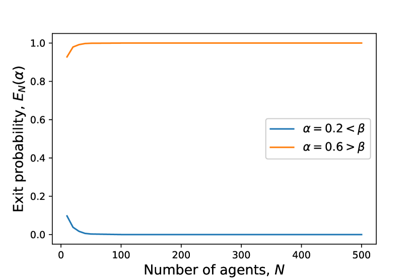
(a) Exit probability $E_{N}(\alpha)$ as a function of the number of agents $N$. Parameters: $q_{0}=1$, $q_{1}=0.6$

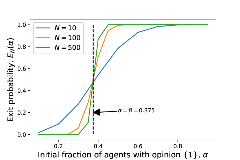
(b) Exit probability $E_{N}(\alpha)$ as a function of the initial fraction $\alpha$ of agents with opinion $\{1\}$. Prameters: $q_{0}=1,q_{1}=0.6$.

Figure 3: Mean consensus time under the voter model with biased agents

In Figure 4(a), we plot the mean consensus time under the majority rule as a function of $N$ for different values of $\alpha$. As predicted by Theorem 4.2, we find that that the mean consensus time is logarithmic in the network size. In Figure 4(b), we study the mean consensus time as a function of $K$ for $q_{0}=1,q_{1}=0.6,\alpha=0.5,N=50$. We observe that with the increase in $K$, the mean time to reach consensus decreases. This is expected since the slope of the mean field $x(t)$ increases with $K$. This leads to faster convergence to the stable equilibrium points.

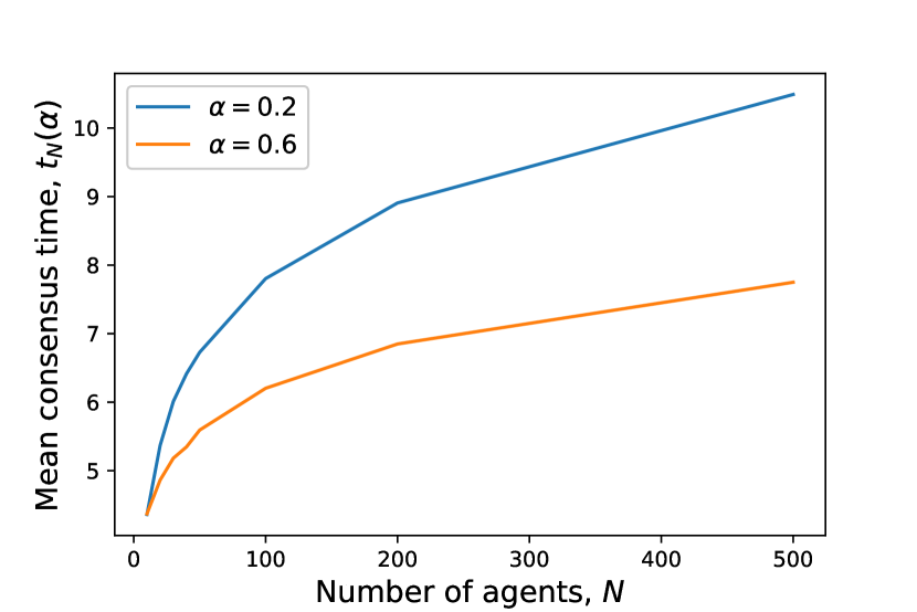
(a) Mean consensus time as a function of $N$. Parameters: $q_{0}=1,q_{1}=0.6,\alpha=0.5$

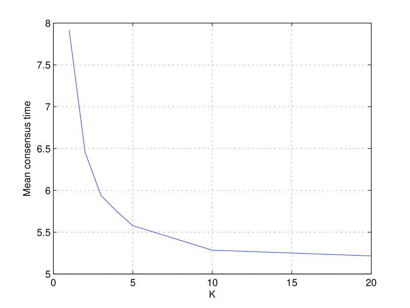
(b) Mean consensus time as a function of $K$. Parameters: $q_{0}=1,q_{1}=0.6,\alpha=0.5,N=50$

Figure 4: Mean consensus time under majority rule with biased agents

5 Majority model with stubborn agents

In this section, we consider the majority rule model in the presence of ‘stubborn agents’. These are agents that never update their opinions. The other agents, referred to as the non-stubborn agents, are assumed to update their opinions at all points of the Poisson processes associated with themselves. We focus on the case where the updates occur according to the majority rule model. The voter model with stubborn agents was studied before in Yildiz_voter_stubborn using coalescing random walks. However, this technique does not apply to the majority rule model. We use mean field techniques to study the opinion dynamics under the majority rule model.

We denote by $\gamma_{i}$, $i\in\{0,1\}$, the fraction of agents in network who are stubborn and have opinion $i$ at all times. Thus, $(1-\gamma_{0}-\gamma_{1})$ is fraction of non-stubborn agents in the network. The presence of stubborn agents prevents the network from reaching a consensus state. This is because at all times there are at least $N\gamma_{0}$ stubborn agents having opinion $\{0\}$ and $N\gamma_{1}$ stubborn agents having opinion $\{1\}$. Furthermore, since each non-stubborn agent may interact with some stubborn agents at every update instant, it is always possible for the non-stubborn agent to change its opinion. Below we characterise the equilibrium fraction of non-stubborn agents having opinion $\{1\}$ in the network for large $N$ using mean field techniques. For analytical tractability, we consider the case $K=1$, i.e., when an agent sample two agents at each update instant. However, similar results hold even for larger values of $K$.

Let $x^{(N)}(t)$ denote the fraction of non-stubborn agents having opinion $\{1\}$ at time $t\geq 0$. Clearly, $x^{(N)}(\cdot)$ is a Markov process with possible jumps at the points of a rate $N(1-\gamma_{0}-\gamma_{1})$ Poisson process. The process $x^{(N)}(\cdot)$ jumps from the state $x$ to the state $x+1/N(1-\gamma_{0}-\gamma_{1})$ when one of the non-stubborn agents having opinion $\{0\}$ becomes active (which happens with rate $N(1-\gamma_{0}-\gamma_{1})(1-x)$) and samples two agents with opinion $\{1\}$. The probability of sampling an agent having opinion $\{1\}$ from the entire network is $(1-\gamma_{0}-\gamma_{1})x+\gamma_{1}$. Hence, the total rate at which the process transits from state $x$ to the state $x+1/N(1-\gamma_{0}-\gamma_{1})$ is given by

$$q\left({x\to x+\frac{1}{N(1-\gamma_{0}-\gamma_{1})}}\right)=N(1-\gamma_{0}-\gamma_{1})(1-x)\\ \times[(1-\gamma_{0}-\gamma_{1})x+\gamma_{1}]^{2}.$$ (16)

Similarly, the rate of the other possible transition is given by

$$q\left({x\to x-\frac{1}{N(1-\gamma_{0}-\gamma_{1})}}\right)=N(1-\gamma_{0}-\gamma_{1})x\\ \times[(1-\gamma_{0}-\gamma_{1})(1-x)+\gamma_{0}]^{2}.$$ (17)

As in Theorem 3.2, it can be shown from the above transition rates that the process $x^{(N)}(\cdot)$ converges weakly to the mean field limit $x(\cdot)$ which satisfies the following differential equation

$$\dot{x}(t)=(1-x(t))[(1-\gamma_{0}-\gamma_{1})x(t)+\gamma_{1}]^{2}\\ -x(t)[(1-\gamma_{0}-\gamma_{1})(1-x(t))+\gamma_{0}]^{2}.$$ (18)

We now study the equilibrium distribution $\pi_{N}$ of the process $x^{(N)}(\cdot)$ for large $N$ via the equilibrium points of the mean field $x(\cdot)$.

From (18) we see that $\dot{x}(t)$ is a cubic polynomial in $x(t)$. Hence, the process $x(\cdot)$ can have at most three equilibrium points in $[0,1]$. We first characterise the stability of these equilibrium points.

Proposition 1

The process $x(\cdot)$ defined by (18) has at least one equilibrium point in $(0,1)$. Furthermore, the number of stable equilibrium points of $x(\cdot)$ in $(0,1)$ is either two or one. If there exists only one equilibrium point of $x(\cdot)$ in $(0,1)$, then the equilibrium point must be globally stable (attractive).

Proof

Define $f(x)=(1-x)[(1-\gamma_{0}-\gamma_{1})x+\gamma_{1}]^{2}-x[(1-\gamma_{0}-\gamma_{1})(1-x)+\gamma_{0}]^{2}$. Clearly, $f(0)=\gamma_{1}^{2}>0$ and $f(1)=-\gamma_{0}^{2}<0$. Hence, there exists at least one root of $f(x)=0$ in $(0,1)$. This proves the existence of an equilibrium point of $x(\cdot)$ in $(0,1)$.

Since $f(x)$ is a cubic polynomial and $f(0)f(1)<0$, either all three roots of $f(x)=0$ lie in $(0,1)$ or exactly one root of $f(x)=0$ lies in $(0,1)$. Let the three (possibly complex and non-distinct) roots of $f(x)=0$ be denoted by $r_{1},r_{2},r_{3}$, respectively. By expanding $f(x)$ we see that the coefficient of the cubic term is $-2(1-\gamma_{0}-\gamma_{1})^{2}$. Hence, $f(x)$ can be written as

$$f(x)=-2(1-\gamma_{0}-\gamma_{1})^{2}(x-r_{1})(x-r_{2})(x-r_{3}).$$ (19)

We first consider the case when $0<r_{1},r_{2},r_{3}<1$ and not all of them are equal. Let us suppose, without loss of generality, that the roots are arranged in the increasing order, i.e., $0<r_{1}\leq r_{2}<r_{3}<1$ or $0<r_{1}<r_{2}\leq r_{3}<1$. From (19) and (18), it is clear that, if $x(t)>r_{2}$ and $x(t)>r_{3}$, then $\dot{x}(t)<0$. Similarly, if $x(t)>r_{2}$ and $x(t)<r_{3}$, then $\dot{x}(t)>0$ . Hence, if $x(0)>r_{2}$ then $x(t)\to r_{3}$ as $t\to\infty$. Using similar arguments we have that for $x(0)<r_{2}$, $x(t)\to r_{1}$ as $t\to\infty$. Hence, $r_{1},r_{3}$ are the stable equilibrium points of $x(\cdot)$. This proves that there exist at most two stable equilibrium points of the mean field $x(\cdot)$.

Now suppose that there exists only one equilibrium point of $x(\cdot)$ in $(0,1)$. This is possible either i) if there exists exactly one real root of $f(x)=0$ in $(0,1)$, or ii) if all the roots of $f(x)=0$ are equal and lie in $(0,1)$. Let $r_{1}$ be a root of $f(x)=0$ in $(0,1)$. Now by expanding $f(x)$ from (19), we see that the product of the roots must be $\gamma_{1}^{2}/2(1-\gamma_{0}-\gamma_{1})^{2}>0$. This implies that the other roots, $r_{2}$ and $r_{3}$, must satisfy one of the following conditions: 1) $r_{2},r_{3}>1$, 2) $r_{2},r_{3}<0$, 3) $r_{2},r_{3}$ are complex conjugates, 4) $r_{2}=r_{3}=r_{1}$.

In all the above cases, we have that $(x-r_{2})(x-r_{3})\geq 0$ for all $x\in[0,1]$ with equality if and only if $x=r_{1}=r_{2}=r_{3}$. Hence, from (19) and (18), it is easy to see that $\dot{x}(t)>0$ when $0\leq x(t)<r_{1}$ and $\dot{x}(t)<0$ when $1\geq x(t)>r_{1}$. This implies that $x(t)\to r_{1}$ for all $x(0)\in[0,1]$. In other words, $r_{1}$ is globally stable.

In the next proposition, we provide the conditions on $\gamma_{0}$ and $\gamma_{1}$ for which there exist multiple stable equilibrium points of the mean field $x(\cdot)$.

Proposition 2

There exist two distinct stable equilibrium points of the mean field $x(\cdot)$ in $(0,1)$ if and only if

1. $D(\gamma_{0},\gamma_{1})=(\gamma_{0}-\gamma_{1})^{2}+3(1-2\gamma_{0}-2\gamma_{1})>0$

2. $0<z_{1},z_{2}<1$, where

   $$z_{1} =\frac{(3-\gamma_{0}-5\gamma_{1})+\sqrt{D(\gamma_{0},\gamma_{1})}}{6(1-\gamma_{0}-\gamma_{1})},$$ (20)

   $$z_{2} =\frac{(3-\gamma_{0}-5\gamma_{1})-\sqrt{D(\gamma_{0},\gamma_{1})}}{6(1-\gamma_{0}-\gamma_{1})}.$$ (21)

3. $f(z_{1})f(z_{2})\leq 0$, where $f(x)=(1-x)[(1-\gamma_{0}-\gamma_{1})x+\gamma_{1}]^{2}-x[(1-\gamma_{0}-\gamma_{1})(1-x)+\gamma_{0}]^{2}$.

If any one of the above conditions is not satisfied then $x(\cdot)$ has a unique, globally stable equilibrium point in $(0,1)$.

Proof

From Proposition 1, we have seen that $x(\cdot)$ has two stable equilibrium points in $(0,1)$ if and only if $f(x)=0$ has three real roots in $(0,1)$ among which at least two are distinct. This happens if and only if $f^{\prime}(x)=0$ has two distinct real roots $z_{1},z_{2}$ in the interval $(0,1)$ and $f(z_{1})f(z_{2})\leq 0$. Since $f^{\prime}(x)$ is a quadratic polynomial in $x$, the above conditions are satisfied if and only if

1. The discriminant of $f^{\prime}(x)=0$ is positive. This corresponds to the first condition of the proposition.

2. The two roots $z_{1},z_{2}$ of $f^{\prime}(x)=0$ must lie in $(0,1)$. This corresponds to the second condition of the proposition.

3. $f(z_{1})f(z_{2})\leq 0$. This is the third condition of the proposition.

Clearly, if any one of the above conditions is not satisfied, then $x(\cdot)$ has a unique equilibrium point in $(0,1)$. According to Proposition 1 this equilibrium point must be globally stable.

Hence, depending on the values of $\gamma_{0}$ and $\gamma_{1}$ there may exist of multiple stable equilibrium points of the mean field $x(\cdot)$. However, for every finite $N$, the process $x^{(N)}(\cdot)$ has a unique stationary distribution $\pi_{N}$ (since it is irreducible on a finite state space). In the next result, we establish that any limit point of the sequence of stationary probability distributions $(\pi_{N})_{N}$ is a convex combination of the Dirac measures concentrated on the equilibrium points of the mean field $x(\cdot)$ in $[0,1]$.

Theorem 5.1

Any limit point of the sequence of probability measures $(\pi_{N})_{N}$ is a convex combination of the Dirac measures concentrated on the equilibrium points of $x(\cdot)$ in $[0,1]$. In particular, if there exists a unique equilibrium point $r$ of $x(\cdot)$ in $[0,1]$ then $\pi_{N}\Rightarrow\delta_{r}$, where $\delta_{r}$ denotes the Dirac measure concentrated at the point $r$.

Proof

We first note that since the sequence of probability measures $(\pi_{N})_{N}$ is defined on the compact space $[0,1]$, it must be tight. Hence, Prokhorov’s theorem implies that $(\pi_{N})_{N}$ is relatively compact. Let $\pi$ be any limit point of the sequence $(\pi_{N})_{N}$. Then by the mean field convergence result we know that $\pi$ must be an invariant distribution of the maps $\alpha\mapsto x(t,\alpha)$ for all $t\geq 0$, i.e., $\int\varphi(x(t,\alpha))d\pi(\alpha)=\int\varphi(\alpha)d\pi(\alpha)$, for all $t\geq 0$, and all continuous (and hence bounded) functions $\varphi:[0,1]\mapsto\mathbb{R}$. In the above, $x(t,\alpha)$ denotes the process $x(\cdot)$ started at $x(0)=\alpha$. Hence we have

$$\int\varphi(\alpha)d\pi(\alpha) =\lim_{t\to\infty}\int\varphi(x(t,\alpha))d\pi(\alpha)$$ (22)

$$=\int\varphi\left({\lim_{t\to\infty}x(t,\alpha)}\right)d\pi(\alpha).$$ (23)

The second equality follows from the first by the Dominated convergence theorem and the continuity of $\varphi$. Now, let $r_{1},r_{2}$, and $r_{3}$ denote the three equilibrium points of the mean field $x(\cdot)$. Hence, by Proposition 1 we have that for each $\alpha\in[0,1]$, $\varphi(\lim_{t\to\infty}x(t,\alpha))=\varphi(r_{1})I_{N_{r_{1}}}(\alpha)+\varphi(r_{2})I_{N_{r_{2}}}(\alpha)+\varphi(r_{3})I_{N_{r_{3}}}(\alpha)$, where for $i=1,2,3$, $N_{r_{i}}\in[0,1]$ denotes the set for which if $x(0)\in N_{r_{i}}$ then $x(t)\to r_{i}$ as $t\to\infty$, and $I$ denotes the indicator function. Hence, by (23) we have that for all continuous functions $\varphi:[0,1]\mapsto\mathbb{R}$

$$\int\varphi(\alpha)d\pi(\alpha)=\varphi(r_{1})\pi(N_{r_{1}})+\varphi(r_{2})\pi(N_{r_{2}})+\varphi(r_{3})\pi(N_{r_{3}}).$$ (24)

This proves that $\pi$ must be of the form $\pi=c_{1}\delta_{r_{1}}+c_{2}\delta_{r_{2}}+c_{3}\delta_{r_{3}}$, where $c_{1},c_{2},c_{3}\in[0,1]$ are such that $c_{1}+c_{2}+c_{3}=1$. This completes the proof.

Thus, according to the above theorem, if there exists a unique equilibrium point of the process $x(\cdot)$ in [0,1], then the sequence of stationary distributions $(\pi_{N})_{N}$ concentrates on that equilibrium point as $N\to\infty$. In other words, for large $N$, the fraction of non-stubborn agents having opinion $\{1\}$ (at equilibrium) will approximately be equal to the unique equilibrium point of the mean field.

Simulation Results: In Figure 5, we plot the equilibrium point of $x(\cdot)$ (when it is unique) as a function of the fraction $\gamma_{1}$ of agents having opinion $\{1\}$ who are stubborn keeping the fraction $\gamma_{0}$ of stubborn agents having opinion $\{0\}$ fixed. We choose the parameter values so that there exists a unique equilibrium point of $x(\cdot)$ in $[0,1]$ (such parameter settings can be obtained using the conditions of Proposition 2). We see that as $\gamma_{1}$ is increased in the range $(0,1-\gamma_{0})$, the equilibrium point shifts closer to unity. This is expected since increasing the fraction of stubborn agents with opinion $\{1\}$ increases the probability with which a non-stubborn agent samples an agent with opinion $\{1\}$ at an update instant.

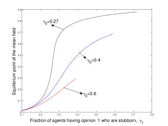
Figure 5: Majority rule with stubborn agents: Equilibrium point of $x(\cdot)$ as a function of $\gamma_{1}$ for different values of $\gamma_{0}$.

If there exist multiple equilibrium points of the process $x(\cdot)$ then the convergence $x^{(N)}(\cdot)\Rightarrow x(\cdot)$ implies that at steady state the process $x^{(N)}(\cdot)$ spends intervals near the region corresponding to one of the stable equilibrium points of $x(\cdot)$. Then due to some rare events, it reaches, via the unstable equilibrium point, to a region corresponding to the other stable equilibrium point of $x(\cdot)$. This fluctuation repeats giving the process $x^{(N)}(\cdot)$ a unique stationary distribution. This behavior is formally known as metastability.

To demonstrate metastability, we simulate a network with $N=100$ agents and $\gamma_{0}=\gamma_{1}=0.2$. For the above parameters, the mean field $x(\cdot)$ has two stable equilibrium points at $0.127322$ and $0.872678$. In Figure 6, we show the sample path of the process $x^{(N)}(\cdot)$. We see that at steady state the process switches back and forth between regions corresponding to the stable equilibrium points of $x(\cdot)$. This provides numerical evidence of the metastable behavior of the finite system.

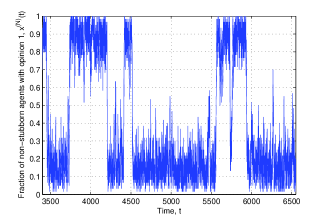
Figure 6: Majority rule with stubborn agents: Sample path of the process $x^{(N)}(\cdot)$ with $N=100$, $\gamma_{0}=\gamma_{1}=0.2$.

6 Proof of Theorem 3.1

Let $T=T_{0}\wedge T_{N}$ denote the random time to reach consensus. Then we have

$$T =\sum_{k=1}^{N-1}\sum_{j=1}^{Z_{k}}M_{k,j},$$ (25)

where $Z_{k}$ denotes the number of visits to state $k$ before absorption and $M_{k,j}$ denotes the time spent in the $j^{\textrm{th}}$ visit to state $k$. Clearly, the random variables $Z_{k}$ and $(M_{k,j})_{j\geq 1}$ are independent with each $M_{k,j}$ being an exponential random variable with rate $(q_{0}+q_{1})k(N-k)/N$. Hence, using Wald’s identity we have

$$t_{N}(\alpha) =\mathbb{E}_{\left\lfloor{\alpha N}\right\rfloor}\left[{T}\right]$$ (26)

$$=\sum_{k=1}^{N-1}\mathbb{E}_{\left\lfloor{\alpha N}\right\rfloor}\left[{Z_{k}}\right]\mathbb{E}_{\left\lfloor{\alpha N}\right\rfloor}\left[{M_{k,j}}\right]$$ (27)

$$=\frac{1}{q_{0}+q_{1}}\sum_{k=1}^{N-1}\left({\frac{1}{k}+\frac{1}{N-k}}\right)\mathbb{E}_{\left\lfloor{\alpha N}\right\rfloor}\left[{Z_{k}}\right].$$ (28)

We now proceed to find lower and upper bounds of $t_{N}(\alpha)$.

Let $A=\left\{{\omega:T_{N}(\omega)<T_{0}(\omega)}\right\}$ denote the event that the Markov chain gets absorbed in state $N$. We have

$$\mathbb{E}_{\left\lfloor{\alpha N}\right\rfloor}\left[{Z_{k}}\right]=\mathbb{E}_{\left\lfloor{\alpha N}\right\rfloor}\left[{Z_{k}|A}\right]\mathbb{P}_{\left\lfloor{\alpha N}\right\rfloor}\left({A}\right) +\mathbb{E}_{\left\lfloor{\alpha N}\right\rfloor}\left[{Z_{k}|A^{c}}\right](1-\mathbb{P}_{\left\lfloor{\alpha N}\right\rfloor}\left({A}\right)).$$ (29)

Lower bound of $t_{N}(\alpha)$: We first obtain a lower bound for $t_{N}(\alpha)$. Clearly, we have the following

$$Z_{k}|A \geq 1\quad\forall k\geq\left\lfloor{\alpha N}\right\rfloor$$

$$Z_{k}|A^{c} \geq 0\quad\forall k>\left\lfloor{\alpha N}\right\rfloor$$

$$Z_{k}|A \geq 0\quad\forall k<\left\lfloor{\alpha N}\right\rfloor$$

$$Z_{k}|A^{c} \geq 1\quad\forall k\leq\left\lfloor{\alpha N}\right\rfloor.$$

Using the above in (29) we have

$$\mathbb{E}_{\left\lfloor{\alpha N}\right\rfloor}\left[{Z_{k}}\right] \geq\mathbb{P}_{\left\lfloor{\alpha N}\right\rfloor}\left({A}\right)\mathbbm{1}_{\left\{{k\geq\left\lfloor{\alpha N}\right\rfloor}\right\}}+(1-\mathbb{P}_{\left\lfloor{\alpha N}\right\rfloor}\left({A}\right))\mathbbm{1}_{\left\{{k\leq\left\lfloor{\alpha N}\right\rfloor}\right\}},$$

where $\mathbbm{1}_{\Omega}$ denotes the indicator function for the set $\Omega$. Using the above in (28), we have

$$t_{N}(\alpha) \geq\frac{\mathbb{P}_{\left\lfloor{\alpha N}\right\rfloor}\left({A}\right)}{q_{0}+q_{1}}\sum_{k=\left\lfloor{\alpha N}\right\rfloor}^{N-1}\left({\frac{1}{k}+\frac{1}{N-k}}\right)+\frac{1-\mathbb{P}_{\left\lfloor{\alpha N}\right\rfloor}\left({A}\right)}{q_{0}+q_{1}}\sum_{k=1}^{\left\lfloor{\alpha N}\right\rfloor}\left({\frac{1}{k}+\frac{1}{N-k}}\right)$$ (30)

$$\geq\frac{1}{q_{0}+q_{1}}\sum_{k=1}^{N(\alpha\wedge(1-\alpha))}\frac{1}{k}$$ (31)

$$>\frac{1}{q_{0}+q_{1}}\log(N(\alpha\wedge(1-\alpha))).$$ (32)

Upper bound for $t_{N}(\alpha)$: We first obtain an upper bound on $\mathbb{E}_{x}\left[{Z_{k};A}\right]$ for $k\geq x$ with any $0<x<N$. Given $A$, let $\zeta_{k}$ denote the number of times the embedded chain $\tilde{X}^{(N)}$ jumps from $k$ to $k-1$ before absorption. It is easy to observe that conditioned on $A$, the embedded chain $\tilde{X}^{(N)}$ is a Markov chain with jump probabilities given by

$$p^{A}_{k,k+1}=1-p^{A}_{k,k-1}=p\frac{\mathbb{P}_{k+1}\left({A}\right)}{\mathbb{P}_{k}\left({A}\right)}\overset{(a)}{=}p\frac{1-r^{k+1}}{1-r^{k}},$$ (33)

where equality (a) follows from Lemma 1. Furthermore, we have

$$Z_{k}|A=1+\zeta_{k}+\zeta_{k+1},\text{ for }x\leq k\leq N-1.$$ (34)

The above relationship follows by observing that the facts that (i) the states $k\geq x$ are visited at least once and (ii) the number of visits to state $k$ is the sum of the numbers of jumps of $\tilde{X}^{(N)}$ to the left and to the right from state $k$.

Given $A$, we must have $\zeta_{N}=0$. Let $\xi_{l,k}$ denote the random number of left-jumps from state $k$ between $l^{\textrm{th}}$ and $(l+1)^{\textrm{th}}$ left-jumps from state $k+1$. Then $(\xi_{l,k})_{l\geq 0}$ are i.i.d with geometric distribution having mean $p^{A}_{k,k-1}/p^{A}_{k,k+1}$. Moreover, we have the following recursion

$$\zeta_{k}=\sum_{l=0}^{\zeta_{k+1}}\xi_{l,k},\text{ for }x\leq k\leq N-1,$$ (35)

(the above sum starts from $l=0$ because for $k\geq x$ left jumps from $j$ can occur even before the chain visits $j+1$ for the first time) Thus, we see that $(\zeta_{k})_{x\leq k\leq N}$ forms a branching process with immigration of one individual in each generation. Applying Wald’s identity to solve the above recursion we have for $x\leq k\leq N-1$

$$\mathbb{E}_{x}\left[{\zeta_{k}}\right] =\sum_{n=k}^{N-1}\prod_{i=k}^{n}\frac{p_{i,i-1}^{A}}{p_{i,i+1}^{A}}$$

$$\overset{(a)}{=}\sum_{n=k}^{N-1}\prod_{i=k}^{n}\frac{r(1-r^{i-1})}{1-r^{i+1}}$$

$$=\frac{r(1-r^{k-1})(1-r^{N-k})}{(1-r)(1-r^{N})},$$ (36)

where equality (a) follows from (33). Taking expectation in (34) and substituting (36) we obtain that for $x\leq k\leq N-1$

$$\mathbb{E}_{x}\left[{Z_{k}|A}\right] =1+\mathbb{E}_{x}\left[{\zeta_{k}}\right]+\mathbb{E}_{x}\left[{\zeta_{k+1}}\right]$$

$$=\frac{1+r}{1-r}\frac{(1-r^{N-k})(1-r^{k})}{1-r^{N}}$$

$$\leq\frac{1+r}{1-r}.$$ (37)

But we also have

$$\mathbb{E}_{x}\left[{Z_{k};A}\right]\leq\mathbb{E}_{x}\left[{Z_{k}|A}\right]\leq\frac{1+r}{1-r}.$$

which provides the required bound on $\mathbb{E}_{x}\left[{Z_{k};A}\right]$. We note that the above bound is independent of $x$. In particular, it is true when $x=\left\lfloor{\alpha N}\right\rfloor$ and $k\geq\left\lfloor{\alpha N}\right\rfloor$.

For $1\leq k<x$ we have

$$\mathbb{E}_{x}\left[{Z_{k};A}\right] =\mathbb{E}_{x}\left[{Z_{k};T_{k}<T_{N}<T_{0}}\right],$$

$$=\mathbb{E}_{x}\left[{Z_{k}|T_{k}<T_{N}<T_{0}}\right]\mathbb{P}_{x}\left({T_{k}<T_{N}<T_{0}}\right),$$

$$\overset{(a)}{=}\mathbb{E}_{k}\left[{Z_{k}|T_{N}<T_{0}}\right]\mathbb{P}_{x}\left({T_{k}<T_{N}<T_{0}}\right),$$

$$\overset{(b)}{\leq}\frac{1+r}{1-r},$$

where the equality $(a)$ follows from the Markov property and inequality $(b)$ follows from (37). Hence, combining all the results above we have that for all $0<k<N$

$$\mathbb{E}_{x}\left[{Z_{k};A}\right]\leq\frac{1+r}{1-r}.$$

Using similar arguments for the process conditioned on $A^{c}$, it follows that for any $0<x<N$ and any $0<k\leq x$ we have

$$\mathbb{E}_{x}\left[{Z_{k};A^{c}}\right] \leq\mathbb{E}_{x}\left[{Z_{k}|A^{c}}\right]$$

$$=\frac{\bar{r}+1}{\bar{r}-1}\frac{(\bar{r}^{N-k}-1)(\bar{r}^{k}-1)}{\bar{r}^{N}-1}$$

$$\leq\frac{1+r}{1-r}.$$

Furthermore, for $N>k>x$ we have

$$\mathbb{E}_{x}\left[{Z_{k};A^{c}}\right] =\mathbb{E}_{x}\left[{Z_{k};T_{k}<T_{0}<T_{N}}\right]$$

$$=\mathbb{E}_{x}\left[{Z_{k}|T_{k}<T_{0}<T_{N}}\right]\mathbb{P}_{x}(T_{k}<T_{0}<T_{N})$$

$$=\mathbb{E}_{k}\left[{Z_{k}|T_{0}<T_{N}}\right]\mathbb{P}_{x}(T_{k}<T_{0}<T_{N})$$

$$\leq\frac{1+r}{1-r}.$$

Combining all the above results we have $\mathbb{E}_{\left\lfloor{\alpha N}\right\rfloor}\left[{Z_{k}}\right]\leq(1+r)/(1-r)$ for all $0<k<N$. Hence from (28) we obtain

$$t_{N}(\alpha) \leq\frac{2}{q_{0}+q_{1}}\frac{1+r}{1-r}\sum_{k=1}^{N-1}\frac{1}{k},$$

$$\leq\frac{2}{q_{0}+q_{1}}\frac{1+r}{1-r}(\log(N-1)+1),$$

which completes the proof.

7 Proof of Theorem 3.2

The process $x^{(N)}(\cdot)$ jumps from the state $x$ to the state $x+1/N$ when one of the $N(1-x)$ agents having opinion $\{0\}$ updates (with probability $q_{0}$) its opinion by interacting with an agent with opinion $\{1\}$. Since the agents update their opinions at points of independent unit rate Poisson processes, the rate at which one of the $N(1-x)$ agents having opinion $\{0\}$ decides to update its opinion is $N(1-x)q_{0}$. The probability with which the updating agent interacts with an agent with opinion $\{1\}$ is $x$. Hence, the total rate of transition from $x$ to $x+1/N$ is given by $r(x\to x+1/N)={q_{0}Nx(1-x)}$. Similarly, the rate of transition from $x$ to $x-1/N$ is given by $r(x\to x-1/N)={q_{1}Nx(1-x)}$. From the above transition rates it can be easily seen that the generator of the process $x^{(N)}(\cdot)$ converges uniformly as $N\to\infty$ to the generator of the deterministic process $x(\cdot)$ defined by (5). From the classical results (see e.g., Kurtz Kurtz_1970 ), the theorem follows.

8 Proof of Lemma 2

We can write $g_{K}(x)=\phi(\psi(x))$, where $\psi(x)=\frac{x}{1-x}:[0,1)\to[0,\infty)$ and

$$\phi(t)=\frac{\sum_{i=K+1}^{2K}\binom{2K}{i}t^{i}}{\sum_{i=K+1}^{2K}\binom{2K}{i}t^{2K+1-i}}=\frac{\sum_{i=K+1}^{2K}\binom{2K}{i}t^{i}}{\sum_{i=1}^{K}\binom{2K}{i-1}t^{i}}.$$

Clearly, $\psi(x):[0,1)\to[0,\infty)$ is strictly increasing. Thus, it is sufficient to show that $\phi:(0,\infty)\to(0,\infty)$ is also strictly increasing. Clearly, $\phi^{\prime}(t)=A(t)/(\sum_{i=1}^{K}\binom{2K}{i-1}t^{i})^{2}$, where

$$A(t) =\left({\sum_{i=K+1}^{2K}i\binom{2K}{i}t^{i-1}}\right)\left({\sum_{i=1}^{K}\binom{2K}{i-1}t^{i}}\right)$$

$$-\left({\sum_{i=K+1}^{2K}\binom{2K}{i}t^{i}}\right)\left({\sum_{i=1}^{K}i\binom{2K}{i-1}t^{i-1}}\right)$$

$$=\sum_{j=K+1}^{3K-1}M_{j}t^{j}$$ (38)

with

$$M_{j}=\sum_{i=\min(1,j+1-2K)}^{\max(K,j-K)}\binom{2K}{i-1}\binom{2K}{j-i+1}(j+1-2i).$$

We note that in the above sum the running variable $i$ satisfies $i\leq\max(K,j-K)$. Furthermore, from (38), we have that $K+1\leq j\leq 3K-1$. Hence, we have $i\leq\max(K,j-K)<\frac{j+1}{2}$ for any $K\geq 1$. This implies that $M_{j}>0$ for all $j$ satisfying $K+1\leq j\leq 3K-1$ Hence, $\phi^{\prime}(t)>0$, $\forall t>0$, which implies that $\phi(t)$ is strictly increasing in $(0,\infty)$.

9 Proof of Theorem 4.1

From the first step analysis of the embedded chain $\tilde{X}^{(N)}(\cdot)$ it follows that

$$E_{N}(n)=p_{n,n+1}E_{N}(n+1)+p_{n,n-1}E_{N}(n-1),$$ (39)

which upon rearranging gives

$$E_{N}(n+1)-E_{N}(n)=\frac{p_{n,n-1}}{p_{n,n+1}}(E_{N}(n)-E_{N}(n-1)).$$ (40)

Putting $D_{N}(n)=E_{N}(n+1)-E_{N}(n)$ we find that (40) reduces to a first order recursion in $D_{N}(n)$ which satisfies the following relation for $1\leq n\leq N-1$

$$D_{N}(n)=r\frac{1}{g_{K}(n/N)}D_{N}(n-1).$$ (41)

To compute $D_{N}(0)$ we use the boundary conditions $E_{N}(0)=0$ and $E_{N}(N)=1$, which imply that $\sum_{n=0}^{N-1}D_{N}(n)=1$. Hence, we have

$$D_{N}(0)=\frac{1}{\sum_{t=0}^{N-1}\prod_{j=1}^{t}\frac{r}{g_{K}(j/N)}},$$ (42)

Thus, using $E_{N}(n)=\sum_{k=0}^{n-1}D_{N}(k)$ we have the required expression for $E_{N}(n)$ for all $0\leq n\leq N$.

It is also important to note that $D_{N}$ defines a probability distribution on the set $\left\{{0,1,\ldots,N-1}\right\}$. Furthermore, using the monotonicity of $g_{K}$ proved in Lemma 2 and (41) we have

$$D_{N}(n) <D_{N}(n-1)\text{ for }n\geq\left\lfloor{\beta N}\right\rfloor+1,$$

$$D_{N}(n) >D_{N}(n-1)\text{ for }n\leq\left\lfloor{\beta N}\right\rfloor.$$

Thus, the mode of the distribution $D_{N}$ is at $\left\lfloor{\beta N}\right\rfloor$. Now for any $\alpha>\beta$ we choose $\beta^{\prime}$ such that $\alpha>\beta^{\prime}>\beta$. Hence, by the monotonicity of $g_{K}$ we have

$$r^{\prime}:=\frac{r}{g_{K}(\beta^{\prime})}<\frac{r}{g_{K}(\beta)}=1.$$

Also using the monotonicity of $g_{K}$ and (41) we have for any $j\geq 1$

$$D_{N}(\left\lfloor{\beta^{\prime}N}\right\rfloor+j) \leq\left({\frac{r}{g_{K}\left({\frac{\left\lfloor{\beta^{\prime}N}\right\rfloor+1}{N}}\right)}}\right)^{j}D_{N}(\left\lfloor{\beta^{\prime}N}\right\rfloor)$$

$$\leq(r^{\prime})^{j}D_{N}(\left\lfloor{\beta^{\prime}N}\right\rfloor),$$

where the last step follows since $\beta^{\prime}N<\left\lfloor{\beta^{\prime}N}\right\rfloor+1$. Hence, we have

$$E_{N}(\alpha) =\sum_{t=0}^{\left\lfloor{\alpha N}\right\rfloor-1}D_{N}(t)$$

$$=1-\sum_{t=\left\lfloor{N\alpha}\right\rfloor}^{N-1}D_{N}(t)$$

$$\geq 1-D_{N}(\left\lfloor{\beta^{\prime}N}\right\rfloor)(r^{\prime})^{\left\lfloor{\alpha N}\right\rfloor-\left\lfloor{\beta^{\prime}N}\right\rfloor}\sum_{t=0}^{N-1-\left\lfloor{\alpha N}\right\rfloor}(r^{\prime})^{t}$$

$$\geq 1-(r^{\prime})^{\left\lfloor{\alpha N}\right\rfloor-\left\lfloor{\beta^{\prime}N}\right\rfloor}\frac{1-(r^{\prime})^{N-\left\lfloor{\alpha N}\right\rfloor}}{1-r^{\prime}}$$

$$\to 1\text{ as }N\to\infty.$$

The proof for $\alpha<\beta$ follows similarly.

10 Proof of Theorem 4.2

Let $T=T_{0}\wedge T_{N}$ denote the random time to reach consensus. Then we have

$$T =\sum_{n=1}^{N-1}\sum_{j=1}^{Z_{n}}M_{n,j},$$ (43)

where $Z_{n}$ denotes the number of visits to state $n$ before absorption and $M_{n,j}$ denotes the time spent in the $j^{\textrm{th}}$ visit to state $n$. Clearly, the random variables $Z_{n}$ and $(M_{n,j})_{j\geq 1}$ are independent with each $M_{n,j}$ being an exponential random variable with rate $q(n\to n+1)+q(n\to n-1)$. Using Wald’s identity we have

$$t_{N}(\alpha) =\mathbb{E}_{\left\lfloor{\alpha N}\right\rfloor}\left[{T}\right]$$

$$=\sum_{n=1}^{N-1}\mathbb{E}_{\left\lfloor{\alpha N}\right\rfloor}\left[{Z_{n}}\right]\mathbb{E}_{\left\lfloor{\alpha N}\right\rfloor}\left[{M_{n,j}}\right]$$

$$=\sum_{n=1}^{N-1}\frac{\mathbb{E}_{\left\lfloor{\alpha N}\right\rfloor}\left[{Z_{n}}\right]}{(q(n\to n+1)+q(n\to n-1))}.$$ (44)

Below we find lower and upper bounds of $t_{N}(\alpha)$. Let $A=\left\{{\omega:T_{N}(\omega)<T_{0}(\omega)}\right\}$ denote the event that the Markov chain gets absorbed in state $N$. We have

$$\mathbb{E}_{\left\lfloor{\alpha N}\right\rfloor}\left[{Z_{n}}\right] =\mathbb{E}_{\left\lfloor{\alpha N}\right\rfloor}\left[{Z_{n}|A}\right]\mathbb{P}_{\left\lfloor{\alpha N}\right\rfloor}\left({A}\right)$$

$$\hskip 20.00003pt+\mathbb{E}_{\left\lfloor{\alpha N}\right\rfloor}\left[{Z_{n}|A^{c}}\right](1-\mathbb{P}_{\left\lfloor{\alpha N}\right\rfloor}\left({A}\right)).$$ (45)

Lower bound of $t_{N}(\alpha)$: Applying Markov inequality to the RHS of (9) and (11) we obtain

$$q(n\to n+1)+q(n\to n-1) \leq(N-n)q_{0}\frac{2K\frac{n}{N}}{K+1}+nq_{1}\frac{2K\left({1-\frac{n}{N}}\right)}{K+1}$$

$$=(q_{0}+q_{1})\frac{2K}{K+1}\frac{N(N-n)}{N}.$$

Furthermore, as in the case of voter model, we have

$$\mathbb{E}_{\left\lfloor{\alpha N}\right\rfloor}\left[{Z_{n}}\right] \geq\mathbb{P}_{\left\lfloor{\alpha N}\right\rfloor}\left({A}\right)\mathbbm{1}_{\left\{{n\geq\left\lfloor{\alpha N}\right\rfloor}\right\}}+(1-\mathbb{P}_{\left\lfloor{\alpha N}\right\rfloor}\left({A}\right))\mathbbm{1}_{\left\{{n\leq\left\lfloor{\alpha N}\right\rfloor}\right\}}.$$

Using (44) and the above inequalities we obtain

$$t_{N}(\alpha) \geq\frac{\mathbb{P}_{\left\lfloor{\alpha N}\right\rfloor}\left({A}\right)}{q_{0}+q_{1}}\frac{K+1}{2K}\sum_{n=\left\lfloor{\alpha N}\right\rfloor}^{N-1}\left({\frac{1}{n}+\frac{1}{N-n}}\right)$$

$$+\frac{1-\mathbb{P}_{\left\lfloor{\alpha N}\right\rfloor}\left({A}\right)}{q_{0}+q_{1}}\frac{K+1}{2K}\sum_{n=1}^{\left\lfloor{\alpha N}\right\rfloor}\left({\frac{1}{n}+\frac{1}{N-n}}\right)$$

$$\geq\frac{1}{q_{0}+q_{1}}\frac{K+1}{2K}\sum_{n=1}^{N(\alpha\wedge(1-\alpha))}\frac{1}{n}$$

$$>\frac{1}{q_{0}+q_{1}}\frac{K+1}{2K}\log(N(\alpha\wedge(1-\alpha))).$$

Upper bound for $t_{N}(\alpha)$: From (9) and (11) we have

$$q(n\to n+1)+q(n\to n-1)\geq\begin{cases}cn,\quad\text{for }\frac{n}{N}\leq\frac{1}{2},\\ c(N-n),\quad\text{for }\frac{n}{N}>\frac{1}{2},\end{cases}$$ (46)

where $c=q_{1}\mathbb{P}\left({\text{Bin}\left({2K,\frac{1}{2}}\right)\geq K+1}\right)$. Using the above inequalities in (44) we have

$$t_{N}(\alpha)\leq\sum_{n=1}^{\left\lfloor{N/2}\right\rfloor}\frac{\mathbb{E}_{\left\lfloor{\alpha N}\right\rfloor}\left[{Z_{n}}\right]}{cn}+\sum_{n=\left\lfloor{N/2}\right\rfloor+1}^{N-1}\frac{\mathbb{E}_{\left\lfloor{\alpha N}\right\rfloor}\left[{Z_{n}}\right]}{c(N-n)}$$ (47)

Hence, to show that $t_{N}(\alpha)=\Theta(\log N)$ it is sufficient to show that $\mathbb{E}_{\left\lfloor{\alpha N}\right\rfloor}\left[{Z_{n}}\right]=O(1)$ for all $1\leq n\leq N-1$.

For the rest of the proof we assume $\alpha>\beta$. The case $\alpha<\beta$ can be handled similarly.

Let $x=\left\lfloor{\alpha N}\right\rfloor$. We first find upper bound of $\mathbb{E}_{x}\left[{Z_{n};A}\right]$. Conditioned on $A$, the embedded chain $\tilde{X}^{(N)}$ is a Markov chain with jump probabilities given by

$$p^{A}_{n,n+1}=1-p^{A}_{n,n-1}=p_{n,n+1}\frac{\mathbb{P}_{n+1}\left({A}\right)}{\mathbb{P}_{n}\left({A}\right)}.$$ (48)

We have

$$\frac{p^{A}_{n,n-1}}{p^{A}_{n,n+1}} =\frac{p_{n,n-1}}{p_{n,n+1}}\frac{\mathbb{P}_{n-1}\left({A}\right)}{\mathbb{P}_{n+1}\left({A}\right)},$$ (49)

$$\overset{(a)}{=}\frac{r}{g_{K}\left({\frac{n}{N}}\right)}\frac{\sum_{t=0}^{n-2}\prod_{j=1}^{t}\frac{r}{g_{K}(j/N)}}{\sum_{t=0}^{n}\prod_{j=1}^{t}\frac{r}{g_{K}(j/N)}},$$ (50)

$$\overset{(b)}{\leq}\min\left({1,\frac{r}{g_{K}\left({\frac{n}{N}}\right)}}\right),$$ (51)

where equality (a) follows from (12) and Theorem 4.1. Inequality (b) follows from the facts (i) $\mathbb{P}_{n-1}\left({A}\right)\leq\mathbb{P}_{n+1}\left({A}\right)$ and (ii) for a monotonically non-increasing non-negative sequence $(y_{n})_{n\geq 1}$ the following inequality holds

$$y_{n}\frac{\sum_{t=0}^{n-2}\prod_{j=1}^{t}y_{j}}{\sum_{t=0}^{n}\prod_{j=1}^{t}y_{j}}\leq 1$$

(follows simply by comparing the terms in the numerator with the middle $n-1$ terms in the denominator).

Given $A$, let $\zeta_{n}$ denote the number of times the embedded chain $\tilde{X}^{(N)}$ jumps from $n$ to $n-1$ before absorption. Then as in the voter model we have

$$Z_{n}|A=\begin{cases}1+\zeta_{n}+\zeta_{n+1},\text{ for }x\leq n\leq N-1,\\ \zeta_{n}+\zeta_{n+1},\text{ for }1\leq n<x,\end{cases}$$ (52)

where $\zeta_{n}$ follows the recursion

$$\zeta_{n}=\begin{cases}\sum_{l=0}^{\zeta_{n+1}}\xi_{l,n},\text{ for }x\leq n\leq N-1,\\ \sum_{l=1}^{\zeta_{n+1}}\xi_{l,n},\text{ for }1\leq n<x\end{cases}$$ (53)

with $\zeta_{N}=0$ and $\xi_{l,n}$ denoting the random number of left-jumps from state $n$ between $l^{\textrm{th}}$ and $(l+1)^{\textrm{th}}$ left-jumps from state $n+1$. Clearly $(\xi_{l,n})_{l\geq 0}$ are i.i.d with geometric distribution having mean $p^{A}_{n,n-1}/p^{A}_{n,n+1}$. Hence, applying Wald’s identity to solve the above recursion we have

$$\mathbb{E}_{x}\left[{\zeta_{n}}\right]=\begin{cases}\sum_{t=n}^{N-1}\prod_{i=n}^{t}\frac{p_{i,i-1}^{A}}{p_{i,i+1}^{A}},\quad\text{for }x\leq n\leq N-1\\ \left({\prod_{i=n}^{x-1}\frac{p_{i,i-1}^{A}}{p_{i,i+1}^{A}}}\right)\mathbb{E}_{x}\left[{\zeta_{x}}\right],\quad\text{for }1\leq n<x.\end{cases}$$ (54)

Now using inequality (51), monotonicity of $g_{K}$, and the fact that for $n\geq x=\left\lfloor{\alpha N}\right\rfloor>\left\lfloor{\beta N}\right\rfloor$, $1>r_{\alpha}:=r/g_{K}(\alpha)\geq r/g_{K}(n/N)$ we have for $n\geq x=\left\lfloor{\alpha N}\right\rfloor$

$$\mathbb{E}_{x}\left[{\zeta_{n}}\right]\leq r_{\alpha}+r_{\alpha}^{2}+\ldots+r_{\alpha}^{N-n}\leq\frac{r_{\alpha}}{1-r_{\alpha}}.$$ (55)

Hence, using (52) we have for $n\geq x=\left\lfloor{\alpha N}\right\rfloor$

$$\mathbb{E}_{x}\left[{Z_{n};A}\right]\leq\mathbb{E}_{x}\left[{Z_{n}|A}\right]\leq\frac{1+r_{\alpha}}{1-r_{\alpha}}=O(1).$$ (56)

For $n<x=\left\lfloor{\alpha N}\right\rfloor$ we have

$$\mathbb{E}_{x}\left[{\zeta_{n}}\right]\overset{(a)}{\leq}\mathbb{E}_{x}\left[{\zeta_{x}}\right]\overset{(b)}{\leq}\frac{r_{\alpha}}{1-r_{\alpha}},$$ (57)

where (a) follows from (54) and (51) and (b) follows from (55). Hence, from (52) we have for $n<x=\left\lfloor{\alpha N}\right\rfloor$

$$\mathbb{E}_{x}\left[{Z_{n};A}\right]\leq\mathbb{E}_{x}\left[{Z_{n}|A}\right]\leq\frac{2r_{\alpha}}{1-r_{\alpha}}=O(1).$$ (58)

Similarly, conditioned on $A^{c}$ we have

$$Z_{n}|A^{c}=\begin{cases}1+\bar{\zeta}_{n}+\bar{\zeta}_{n-1}\text{ for }1\leq n\leq x,\\ \bar{\zeta}_{n}+\bar{\zeta}_{n-1}\text{ for }x<n<N-1,\end{cases}$$ (59)

where $\bar{\zeta}_{n}$ denotes the number of times $\tilde{X}^{(N)}$ jumps to the right from state $n$ given $A^{c}$. Hence, $\bar{\zeta}_{n}$ follows the recursion given by

$$\bar{\zeta}_{n}=\begin{cases}\sum_{l=0}^{\bar{\zeta}_{n-1}}\bar{\xi}_{l,n},\text{ for }1\leq n\leq x,\\ \sum_{l=1}^{\bar{\zeta}_{n-1}}\bar{\xi}_{l,n},\text{ for }x<n<N-1\end{cases}$$ (60)

where $\bar{\zeta}_{0}=0$ and $\bar{\xi}_{l,n}$ denotes the random number of right-jumps from state $n$ between $l^{\textrm{th}}$ and $(l+1)^{\textrm{th}}$ right-jumps from state $n-1$ given $A^{c}$. Clearly $(\bar{\xi}_{l,n})_{l\geq 0}$ are i.i.d. with geometric distribution having mean $p^{A^{c}}_{n,n+1}/p^{A^{c}}_{n,n-1}$ where

$$p^{A^{c}}_{n,n+1}=1-p^{A^{c}}_{n,n-1}=p_{n,n+1}\frac{\mathbb{P}_{n+1}\left({A^{c}}\right)}{\mathbb{P}_{n}\left({A^{c}}\right)}.$$ (61)

As before, we have

$$\frac{p^{A^{c}}_{n,n+1}}{p^{A^{c}}_{n,n-1}} {=}\frac{g_{K}\left({\frac{n}{N}}\right)}{r}\frac{\sum_{t=n+1}^{N-1}\prod_{j=t+1}^{N-1}\frac{g_{K}(j/N)}{r}}{\sum_{t=n-1}^{N-1}\prod_{j=t+1}^{N-1}\frac{g_{K}(j/N)}{r}}{\leq}\min\left({1,\frac{g_{K}\left({\frac{n}{N}}\right)}{r}}\right),$$ (62)

Solving (60) using Wald’s identity we obtain

$$\mathbb{E}_{x}\left[{\bar{\zeta}_{n}}\right]=\begin{cases}\sum_{t=1}^{n}\prod_{i=t}^{n}\frac{p_{i,i+1}^{A^{c}}}{p_{i,i-1}^{A^{c}}},\quad\text{for }1\leq n\leq x,\\ \left({\prod_{i=x+1}^{n}\frac{p_{i,i+1}^{A^{c}}}{p_{i,i-1}^{A^{c}}}}\right)\mathbb{E}_{x}\left[{\bar{\zeta}_{x}}\right],\quad\text{for }x<n<N-1.\end{cases}$$ (63)

For $1\leq n\leq x$ after some simplification of (63) we obtain

$$\mathbb{E}_{x}\left[{\bar{\zeta}_{n}}\right]=\frac{\prod_{j=1}^{n}\frac{g_{K}(j/N)}{r}}{\prod_{j=1}^{N-1}\frac{g_{K}(j/N)}{r}}\mathbb{P}_{n+1}\left({A^{c}}\right)\left({1-\mathbb{P}_{n}\left({A^{c}}\right)}\right).$$ (64)

We observe that for $j\leq\left\lfloor{\beta N}\right\rfloor$ we have $\frac{g_{K}(j/N)}{r}\leq 1$ and using the fact that $g_{K}(x)=1/g_{K}(1-x)$ we have $\prod_{j=1}^{N-1}\frac{g_{K}(j/N)}{r}=1/r^{N-1}$. Hence, using (64) for $n\leq\left\lfloor{\beta N}\right\rfloor$ we have

$$\mathbb{E}_{x}\left[{\bar{\zeta}_{n}}\right]\leq\frac{\prod_{j=1}^{n}\frac{g_{K}(j/N)}{r}}{\prod_{j=1}^{N-1}\frac{g_{K}(j/N)}{r}}\leq r^{N-1}\leq 1.$$ (65)

Furthermore, for $\left\lfloor{\beta N}\right\rfloor<n\leq x$ we have

$$\mathbb{E}_{x}\left[{\bar{\zeta}_{n}}\right]\leq\frac{1}{\prod_{j=n+1}^{N-1}\frac{g_{K}(j/N)}{r}}\overset{(a)}{\leq}1,$$ (66)

where (a) follows from the fact that $\frac{g_{K}(j/N)}{r}\geq 1$ for $j>n>\left\lfloor{\beta N}\right\rfloor$. Hence, we have shown that $\mathbb{E}_{x}\left[{\bar{\zeta}_{n}}\right]=O(1)$ for $1\leq n\leq x$. Now, using (63) and inequality (62) we have for $x<n<N-1$ that $\mathbb{E}_{x}\left[{\bar{\zeta}_{n}}\right]\leq\mathbb{E}_{x}\left[{\bar{\zeta}_{x}}\right]=O(1)$. Hence, from (59) we see that $\mathbb{E}_{x}\left[{Z_{n};A^{c}}\right]\leq\mathbb{E}_{x}\left[{Z_{n}|A^{c}}\right]=O(1)$ thereby completing the proof.

11 Conclusion

In this paper, we analysed the voter model the majority rule model of social interaction under the presence of biased and stubborn agents. We observed that for the voter model the presence of biased agents, reduces the mean consensus time exponentially in comparison to the voter model with unbiased agents. For the majority rule model with biased agents, we saw that the network reaches the consensus state with all agents adopting the preferred opinion only if the initial fraction of agents having the preferred opinion is more than a certain threshold value. Finally, we have seen that for the majority rule model with stubborn agents the network exhibits metastability, where it fluctuates between multiple stable configuration, spending long intervals in each configuration.

Several interesting directions for future work exist. For example, the behaviour of random $d$-regular networks under the biased voter and majority rule models has not been analysed yet. Furthermore, the effect of the presence of more than two opinion on the opinion dynamics is unknown. It will be also interesting to study the networks dynamics under the majority rule model for general network topologies when stubborn agents are present.

References

• (1) Agur, Z., Fraenkel, A., Klein, S.: The number of fixed points of the majority rule. Discrete Mathematics 70(3), 295 – 302 (1988)
• (2) Bandyopadhyay, A., Roy, R., Sarkar, A.: On the one dimensional learning from neighbours model. Electronic Journal of Probability 15(51), 1574–1593 (2010)
• (3) Becchetti, L., Clementi, A., Natale, E.: Consensus dynamics: An overview. SIGACT News 51(1), 58–104 (2020). DOI 10.1145/3388392.3388403
• (4) Chatterjee, K., Xu, S.H.: Technology diffusion by learning from neighbours. Advances in Applied Probability 36(2), 355–376 (2004)
• (5) Chen, P., Redner, S.: Consensus formation in multi-state majority and plurality models. Journal of Physics A: Mathematical and General 38(33), 7239 (2005)
• (6) Chen, P., Redner, S.: Majority rule dynamics in finite dimensions. Physical Review E 71(3), 036101 (2005)
• (7) Clifford, P., Sudbury, A.: A model for spatial conflict. Biometrika 60(3), 581–588 (1973)
• (8) Cooper, C., Elsässer, R., Radzik, T.: The power of two choices in distributed voting. In: J. Esparza, P. Fraigniaud, T. Husfeldt, E. Koutsoupias (eds.) Automata, Languages, and Programming, pp. 435–446. Springer Berlin Heidelberg, Berlin, Heidelberg (2014)
• (9) Cooper, C., Elsässer, R., Ono, H., Radzik, T.: Coalescing random walks and voting on connected graphs. SIAM Journal on Discrete Mathematics 27(4), 1748–1758 (2013). DOI 10.1137/120900368
• (10) Cox, J.T.: Coalescing random walks and voter model consensus times on the torus in $\mathbb{Z}^{d}$. Annals of Probability 17(4), 1333–1366 (1989)
• (11) Cruise, J., Ganesh, A.: Probabilistic consensus via polling and majority rules. Queueing Syst. Theory Appl. 78(2), 99–120 (2014). DOI 10.1007/s11134-014-9397-7
• (12) DeGroot, M.H.: Reaching a consensus. Journal of the American Statistical Association 69(345), 118–121 (1974)
• (13) Ellison, G., Fudenberg, D.: Rules of thumb for social learning. Journal of Political Economy 101(4), 612–643 (1993)
• (14) Flocchini, P., Lodi, E., Luccio, F., Pagli, L., Santoro, N.: Dynamic monopolies in tori. Discrete Applied Mathematics 137(2), 197–212 (2004)
• (15) Galam, S.: Minority opinion spreading in random geometry. European Journal of Physics 25(4), 403–406 (2002)
• (16) Gast, N., Gaujal, B.: Computing absorbing times via fluid approximations. Advances in Applied Probability 49(3) (2017)
• (17) Hassin, Y., Peleg, D.: Distributed probabilistic polling and applications to proportionate agreement. Inf. Comput. 171(2), 248–268 (2002). DOI 10.1006/inco.2001.3088. URL https://doi.org/10.1006/inco.2001.3088
• (18) Holley, R.A., Liggett, T.M.: Ergodic theorems for weakly interacting infinite systems and the voter model. Annals of Applied Probability 3(4) (1975)
• (19) Krapivsky, P.L.: Kinetics of monomer-monomer surface katalytic reactions. Physical Review A 45(2) (1992)
• (20) Krapivsky, P.L., Redner, S.: Dynamics of majority rule in two-state interacting spin systems. Physical Review Letters 90(23), 238701 (2003)
• (21) Kurtz, T.G.: Solutions of ordinary differential equations as limits of pure jump markov processes. Journal of Applied Probability 7(1), 49–58 (1970)
• (22) Mobilia, M., Petersen, A., Redner, S.: On the role of zealotry in the voter model. Journal of Statistical Mechanics: Theory and Experiment 2007(8), P08029 (2007)
• (23) Moran, G.: The r-majority vote action on 0–-1 sequences. Discrete Mathematics 132(1), 145 – 174 (1994)
• (24) Mossel, E., Neeman, J., Tamuz, O.: Majority dynamics and aggregation of information in social networks. Autonomous Agents and Multi-Agent Systems 28(3), 408–429 (2014)
• (25) Mukhopadhyay, A., Mazumdar, R.R., Roy, R.: Binary opinion dynamics with biased agents and agents with different degrees of stubbornness. In: 2016 28th International Teletraffic Congress (ITC 28), vol. 01, pp. 261–269 (2016). DOI 10.1109/ITC-28.2016.143
• (26) Nakata, T., Imahayashi, H., Yamashita, M.: Probabilistic local majority voting for the agreement problem on finite graphs. In: T. Asano, H. Imai, D.T. Lee, S.i. Nakano, T. Tokuyama (eds.) Computing and Combinatorics, pp. 330–338. Springer Berlin Heidelberg, Berlin, Heidelberg (1999)
• (27) Perron, E., Vasudevan, D., Vojnovic, M.: Using three states for binary consensus on complete graphs. In: IEEE INFOCOM 2009, pp. 2527–2535 (2009). DOI 10.1109/INFCOM.2009.5062181
• (28) Sood, V., Redner, S.: Voter model on heterogeneous graphs. Physical Review Letters 94(17) (2005)
• (29) Spitzer, F.: Principles of Random Walks. Springer, New York (1964)
• (30) Tsitsiklis, J.N.: Problems in decentralized decision making and computation. Ph.D. thesis, M.I.T (1984)
• (31) Yildiz, E., Ozdaglar, A., Acemoglu, D., Saberi, A., Scaglione, A.: Binary opinion dynamics with stubborn agents. ACM Transactions on Economics and Computation 1(4), 1–30 (2013)
• (32) Yildiz, M.E., Pagliary, R., Ozdaglar, A., Scaglione, A.: Voting models in random networks. In: Information Theory and Applications Workshop (ITA), pp. 1–7 (2010)