Convex Optimization Over Risk-Neutral Probabilities

Abstract

We consider a collection of derivatives that depend on the price of an underlying asset at expiration or maturity. The absence of arbitrage is equivalent to the existence of a risk-neutral probability distribution on the price; in particular, any risk neutral distribution can be interpreted as a certificate establishing that no arbitrage exists. We are interested in the case when there are multiple risk-neutral probabilities. We describe a number of convex optimization problems over the convex set of risk neutral price probabilities. These include computation of bounds on the cumulative distribution, VaR, CVaR, and other quantities, over the set of risk-neutral probabilities. After discretizing the underlying price, these problems become finite dimensional convex or quasiconvex optimization problems, and therefore are tractable. We illustrate our approach using real options and futures pricing data for the S&P 500 index and Bitcoin.

1 Introduction

The arbitrage theorem is a central result in finance originally proposed by Ross [31]. For a market with a finite number of investments and possible outcomes, the arbitrage theorem states that there either exists a probability distribution (called a risk-neutral probability) over the outcomes such that the expected return of all possible investments is nonpositive (i.e., arbitrage does not exist), or there exists a nonnegative combination of the investments that guarantees positive expected return (i.e., arbitrage exists). The no-arbitrage assumption is that financial markets are arbitrage-free. For the most part, this holds, since if the markets were not arbitrage-free, someone would take advantage of the arbitrage, changing the price until it no longer exists. Under the no-arbitrage assumption, a notable implication of the arbitrage theorem is that a risk-neutral probability serves both as a conceivable distribution over the outcomes and as a certificate ensuring that arbitrage is impossible.

For a given market, the set of risk-neutral probabilities is a polyhedron, and arbitrage is impossible if the set is nonempty. We can verify that the market is arbitrage-free by finding a point in the feasible set of a particular system of linear equalities. Apart from verifying the no-arbitrage assumption, this set has many other uses. For example, it has been used for projecting onto the set of risk-neutral probabilities using various distance measures (e.g., $\ell_{2}$ norm, $\ell_{1}$ norm, and KL-divergence) [32, 27, 33, 11, 24, 10], as well as for computing bounds on option prices given moments or other information [7, 6, 26]. These methods have been applied to various derivative markets, including equity indices [5, 3], currencies [12], and commodities [28]. We consider nonparametric models of risk-neutral probabilities in this paper; another viable option is to consider parametric models, i.e., choose a distribution and fit its parameters to observed pricing data (see, e.g., [bahra1a997implied, 24] and the references therein). We note that once a risk-neutral distribution is found, it is often used to construct stochastic processes of the price of the underlying asset, e.g., as a binomial tree [32, 23]. Risk-neutral probabilities have also been used to infer properties of investor’s utility functions [4, 25].

In this paper we consider the general problem of minimizing a convex or quasiconvex function over the (convex) set of risk-neutral probabilities. By considering convex optimization problems, finding a solution is tractable, and indeed has linear complexity in the number of outcomes, which lets us scale the number of outcomes to the tens of thousands. Moreover, the advent of domain-specific languages (DSLs) for convex optimization, e.g., CVXPY [15, 2], make not just solving, but also formulating these problems straightforward; they require just a few lines of a high-level language such as Python. We show that there are many useful applications of convex optimization problems over risk-neutral probabilities, which encompass a lot of prior work, including computation of bounds on expected values of arbitrary functions of the expiration price, estimation of the risk-neutral probability using other information, computation of bounds on the cost of existing or new investments, and sensitivities of various quantities to the cost of each investment. We illustrate a number of these applications using real derivatives pricing data for the S&P 500 index and Bitcoin.

There are a number of notable limitations to our approach. First, we require the number of outcomes to be finite and reasonably small. Suppose, e.g., that we tried to apply our approach to American-style options, which can be exercised at any time up until to expiration. Even if we discretized the price of the underlying asset and time, the number of outcomes would be exponentially large, since we would need to consider the price of the asset at each time point until expiration. (We note however that precise valuation and optimal exercise of American options is still mostly an unsolved problem.) Second, we consider static investments, i.e., the investment is fixed until expiration. This precludes multi-period investment models [16], dynamic hedging strategies that are at the core of derivative pricing models like the Black-Scholes model [8, 29], as well as treatment of American options, since we need to decide whether to exercise an option or not based on the current price. Despite these limitations, we find that our approach can be very useful in practice and is also very interpretable, as demonstrated by our examples in §4.

Outline.

The remainder of the paper is organized as follows. In §2 we describe the setting of the paper, define risk-neutral probabilities, and give a characterization of the set of risk-neutral probabilities. In §3 we present the problem of convex optimization over risk-neutral probabilities and give a number of applications of this problem. Finally, in §4, we illustrate our approach on real derivatives pricing data for the S&P 500 Index and Bitcoin.

2 Risk-neutral probabilities

Setting.

We consider a market for an asset, referred to as the underlying, with a number of derivatives that provide payoffs at the same future date or time, referred to as expiration or maturity. We assume that there are $n$ possible investments that include, e.g., buying or (short) selling the underlying, as well as buying or selling (writing) derivatives. We let $p>0$ denote the price of the underlying at expiration.

Payoff.

The payoff function $f_{i}:{\mbox{\bf R}}_{+}\to{\mbox{\bf R}}$ denotes the dollar amount received (or paid, if negative) per unit held of the $i$th investment; we give some examples of payoff functions below. If we own a quantity $w_{i}\geq 0$ of the $i$th investment, then at expiration, we would receive $f_{i}(p)w_{i}$ dollars. (We note that we do not discount payoffs at the risk-free rate, but we could easily do this in our formulation.)

Cost.

We let $c\in{\mbox{\bf R}}^{n}$ denote the cost in dollars to acquire one unit of each investment ($c_{i}<0$ means that we are paid to acquire the investment). The cost is the ask price if we are purchasing and the negative bid price if we are selling, adjusted for fees and rebates. If we acquired a quantity $w_{i}\geq 0$ of the $i$th investment, it would cost us $c_{i}w_{i}$ dollars, and the return of our investment, at expiration, would be $(f_{i}(p)-c_{i})w_{i}$ dollars.

2.1 Examples of payoff functions

In this section we give some examples of payoff functions (see, e.g., [22] for an overview of various derivatives).

Underlying.

In many cases we can directly invest in the underlying. We allow both going long (buying), and going short (selling borrowed shares). Going long in the underlying has a payoff function

$$f(p)=p,$$

and going short in the underlying has the payoff function

$$f(p)=-p.$$

European options.

A European option is a contract that gives one party the right to buy or sell an underlying asset at an agreed upon strike price. If the right is to buy the underlying asset (a call option), the option will only be exercised if the underlying price is greater than the strike price. Conversely, if the right is to sell the underlying asset (a put option), the option will only be exercised if the underlying price is less than the strike price. Under this logic, the payoff functions for buying European options with a strike price $s$ are

$$f^{\mathrm{call}}(p)=(p-s)_{+},\quad f^{\mathrm{put}}(p)=(p-s)_{-},$$

where $x_{+}=\max(x,0)$ and $x_{-}=(-x)_{+}$. The payoff function for selling (writing) a European option is

$$f^{\mathrm{w,call}}(p)=-f^{\mathrm{call}}(p),\quad f^{\mathrm{w,put}}(p)=-f^{\mathrm{put}}(p).$$

Futures.

Futures are contracts that obligate the buyer of the contract to buy or sell the underlying asset at an agreed upon strike price. A long futures contract means the party must buy the underlying asset at that strike price. Denoting the strike price of the future by $s$, the payoff for buying a long futures contract is

$$f(p)=p-s.$$

A short futures contract means the party must sell the underlying asset at that strike price. The return function for buying a short futures contract is

$$f(p)=s-p.$$

Binary options.

A binary option is a contract that pays either a fixed monetary amount or nothing depending on the underlying’s price. For example, a binary option that pays the buyer one dollar if the underlying asset is above a strike price $s$ has a payoff function

$$f(p)=\begin{cases}1&p\geq s,\\ 0&\text{otherwise}.\end{cases}$$

If we sell that same binary option, the payoff function is

$$f(p)=\begin{cases}-1&p\geq s,\\ 0&\text{otherwise}.\end{cases}$$

2.2 Discretized outcomes

For the remainder of the paper we will work with a discretized version of the price $p$, meaning it can only take one of $m$ values $p_{1},\ldots,p_{m}$, where we assume $p_{1}<p_{2}<\cdots<p_{m}$. (We note that the discretization can be unequally spaced.) Since the methods that we describe involve convex optimization, they scale well (and often linearly) with $m$ [9]; this implies that $m$ can be chosen to be large enough that the discretization error is negligible.

We can define a probability distribution over $p$ as a vector $\pi\in{\mbox{\bf R}}^{m}$, with $\mathop{\bf Prob}(p=p_{i})=\pi_{i}$. Such a vector is in the set

$$\Delta=\{\pi\in{\mbox{\bf R}}^{m}\mid\pi\geq 0,~{}\mathbf{1}^{T}\pi=1\},$$

i.e., the probability simplex in ${\mbox{\bf R}}^{m}$.

2.3 The set of risk-neutral probabilities

Payoff matrix.

We can summarize the payoffs of each investment for each possible outcome with the payoff matrix $P\in{\mbox{\bf R}}^{m\times n}$, with entries given by

$$P_{ij}=f_{j}(p_{i}),\quad i=1,\ldots,m,\quad j=1,\ldots,n.$$

Here $P_{ij}$ is the payoff in dollars per unit invested in investment $j$, if outcome $i$ occurs.

Arbitrage.

Let $w\in{\mbox{\bf R}}_{+}^{n}$ denote an investment vector, meaning we invest in a quantity $w_{i}$ of the $i$th investment, and hold these investments until expiration. The overall investment will cost us $c^{T}w$ now, and our expected payoff at expiration will be $\pi^{T}Pw$, meaning our expected return is $(P^{T}\pi-c)^{T}w$. Arbitrage is said to exist if there exists an investment vector that guarantees positive expected return, i.e., there exists $w\geq 0$ with $(P^{T}\pi-c)^{T}w>0$. Equivalently, arbitrage is said to exist if the homogeneous linear program (LP)

$$\begin{array}[]{ll}\mbox{maximize}&(P^{T}\pi-c)^{T}w\\ \mbox{subject to}&w\geq 0,\end{array}$$ (1)

with variable $w$, is unbounded above.

The set of risk-neutral probabilities.

We say that $\pi$ is a risk-neutral probability (or no-arbitrage distribution) if arbitrage is impossible, that is, if the optimal value of problem (1) is bounded. By LP duality [13] or the Farkas lemma [18], (1) is bounded if and only if $P^{T}\pi\leq c$. This means that the set of risk-neutral probabilities is the (convex) polyhedron

$$\Pi=\{\pi\in\Delta\mid P^{T}\pi\leq c\}.$$

We note that if $\Pi$ is empty, then arbitrage exists. We can interpret $\pi\in\Pi$ as a distribution over the outcomes for which it is impossible to invest and receive positive expected return.

Another interpretation.

Consider the problem

$$\begin{array}[]{ll}\mbox{maximize}&t\\ \mbox{subject to}&Pw-(c^{T}w)\mathbf{1}\geq t\mathbf{1},\\ &w\geq 0,\end{array}$$ (2)

with variable $w$. (This problem is equivalent to problem (1).) If it is unbounded above, then for every $R>0$, there exists an investment vector $w$ that guarantees our return will be at least $R$, no matter what the outcome is. The dual is

$$\begin{array}[]{ll}\mbox{maximize}&0\\ \mbox{subject to}&\pi\in\Pi,\end{array}$$ (3)

with variable $\pi$. Therefore, another interpretation of $\pi\in\Pi$ is as a certificate guaranteeing that it is impossible to always have positive return regardless of the outcome.

Example.

Suppose there are $n=2$ investments, $m=2$ outcomes, the prices are $c=(1,1)$, and the payoff matrix is

$$P=\begin{bmatrix}3/2&0\\ 1/2&3/2\end{bmatrix}.$$

Then the set of risk-neutral probability distributions is

$$\Pi=\{(x,1-x)\mid 1/3\leq x\leq 1/2\}.$$

We visualize the construction of this set in figure 1.

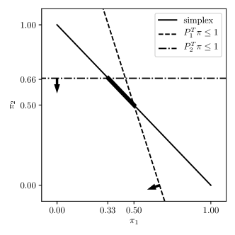
Figure 1: An example of the set of risk-neutral probabilities $\Pi$, denoted by the thick line segment. Here $P_{i}$ denotes the $i$th column of $P$.

3 Convex optimization over risk-neutral probabilities

The general problem of convex optimization over risk-neutral probabilities is

$$\begin{array}[]{ll}\mbox{minimize}&L(\pi)\\ \mbox{subject to}&\pi\in\Pi,\end{array}$$ (4)

with variable $\pi$, where $L:{\mbox{\bf R}}^{m}\to{\mbox{\bf R}}\cup\{+\infty\}$ is convex (or quasiconvex). We use infinite values of $L$ to encode constraints. $\Pi$ is a polyhedron, so (4) is a convex optimization problem [9]. In general problem (4) does not have an analytical solution, but we can numerically find the global optimum efficiently using modern convex optimization solvers [9]. All of the problems we describe below (and many others) are readily expressed in a few lines of code using domain specific languages for convex optimization, such as CVX [20, 21], CVXPY [15, 2], Convex.jl [34], or CVXR [19].

3.1 Functions of the price

Suppose $g:{\mbox{\bf R}}\to{\mbox{\bf R}}$ is some function of the underlying’s price at expiration; the expectation of $g$ is

$$\mathop{\bf E{}}g(p)=\sum_{i=1}^{m}\pi_{i}g(p_{i}),$$

which is a linear function of $\pi$. Some examples of functions of the price include:

• The price. Here $g(p)=p$. The expected value is the expected price.

• The return on an investment. Here $g(p)=\sum_{i=1}^{n}(f_{i}(p)-c_{i})w_{i}$ for an investment $w\in{\mbox{\bf R}}_{+}^{n}$. The expected value is the expected return of the investment.

• Indicator functions of arbitrary sets. Here $g(p)=1$ if $p\in C$ and 0 otherwise, for some set $C\subseteq{\mbox{\bf R}}$. The expected value is $\mathop{\bf Prob}(p\in C)$.

Bounds on expected values.

We can compute lower and upper bounds on expected values of functions of the price by respectively letting $L(\pi)=\mathop{\bf E{}}g(p)$ and $L(\pi)=-\mathop{\bf E{}}g(p)$ and solving problem (4). For example, we could compute bounds on the expected price or the return on a given investment.

Bounds on ratios of expected values.

If we have another function $f$ of the price, and $g(p)>0$, then the function

$$\frac{\mathop{\bf E{}}f(p)}{\mathop{\bf E{}}g(p)}=\frac{\sum_{i}\pi_{i}f(p_{i})}{\sum_{i}\pi_{i}g(p_{i})},$$

is quasilinear. We can find bounds on this ratio by minimizing and maximizing this quantity, both of which are both quasiconvex optimization problems. For example, we can compute bounds on $\mathop{\bf Prob}(p\in A\mid p\in B)$ for two sets $A\subseteq{\mbox{\bf R}}$ and $B\subseteq{\mbox{\bf R}}$, since it is equal to

$$\frac{\mathop{\bf Prob}(p\in A\cap B)}{\mathop{\bf Prob}(p\in B)}.$$

CDF.

The cumulative distribution function (CDF) of $g$ is the function

$$F(x)=\mathop{\bf Prob}(g(p)\leq x)=\sum_{g(p_{i})\leq x}\pi_{i},$$

which, for each $x$, is linear in $\pi$. For example, if $g(p)=p$, then $F(x)$ is just the CDF of the price. We can compute lower and upper bounds on the CDF at $x=p_{1},\ldots,p_{m},$ by minimizing and maximizing $F(x)$ subject to $\pi\in\Pi$.

VaR.

The value-at-risk of $g(p)$ at probability $\epsilon\in[0,1]$ is defined as

$$\mathbf{VaR}(g(p);\epsilon)=\inf\{\alpha\mid\mathop{\bf Prob}(g(p)\leq\alpha)\geq\epsilon\}=F^{-1}(\epsilon),$$

where $F^{-1}(\epsilon)=\inf\{x\mid F(x)\geq\epsilon\}$ [17]. From the bounds on the CDF, we can compute bounds on the value at risk as

$$F_{\mathrm{max}}^{-1}(\epsilon)\leq\mathbf{VaR}(g(p);\epsilon)\leq F_{\mathrm{min}}^{-1}(\epsilon).$$

CVaR.

The conditional value-at-risk of $g(p)$ at probability $\epsilon$ is defined as (see, e.g., [30])

$$\mathbf{CVaR}(g(p);\epsilon)=\inf_{\beta}\left(\beta+\frac{\mathop{\bf E{}}(g(p)-\beta)_{+}}{1-\epsilon}\right)=\min_{i}\left(p_{i}+\sum_{j=1}^{m}\pi_{j}\frac{(g(p_{j})-p_{i})_{+}}{1-\epsilon}\right),$$

which is a concave function of $\pi$. Therefore, we can find an upper bound on $\mathbf{CVaR}$ by letting $L(\pi)=-\mathbf{CVaR}(g(p);\epsilon)$. Since conditional value-at-risk is bounded below by value-at-risk, $F_{\mathrm{max}}^{-1}(\epsilon)$ is a (trivial) lower bound.

Constraints.

We can incorporate upper or lower bounds on the expected values of functions of the price as linear equality constraints in the function $L$. These linear inequality constraints can be interpreted as adding another investment. For example, if we add the constraint $a^{T}\pi\leq b$ for $a\in{\mbox{\bf R}}^{m}$ and $b\in{\mbox{\bf R}}$, this is the same as if we had originally included an investment with a payoff function $f(p_{i})=a_{i}$ and cost $b$.

3.2 Estimation

Maximum entropy.

We can find the maximum entropy risk-neutral probability by letting

$$L(\pi)=\sum_{i=1}^{m}\pi_{i}\log(\pi_{i}).$$

Minimum KL-divergence.

Given another distribution $\eta\in\Delta$, we can find the closest risk-neutral probability distribution to $\eta$ as measured by Kullback-Leibler (KL) divergence by letting

$$L(\pi)=\sum_{i=1}^{m}\pi_{i}\log(\pi_{i}/\eta_{i}).$$

Closest log-normal distribution.

We can approximately find the closest log-normal distribution to $\Pi$ by performing the following alternating projection procedure, starting with $\pi_{0}\in\Pi$:

• Fit a log-normal distribution to $\pi_{k}$ with mean and variance

  $$\mu=\sum_{i=1}^{m}\pi_{i}\log(p_{i}),\quad\sigma^{2}=\sum_{i=1}^{m}\pi_{i}(\log(p_{i})-\mu)^{2}.$$

• Discretize this distribution, resulting in $\eta_{k}\in\Delta$.

• Set $\pi_{k+1}$ equal to the closest risk-neutral probability distribution to $\eta_{k}$, in terms of KL-divergence. If $\pi_{k+1}$ is close enough to $\eta_{k}$, then quit.

For better performance, this process may be repeated for various $\pi_{0}\in\Pi$.

3.3 Bounds on costs

Suppose that we want to add another investment, and would like to come up with lower and upper bounds on its cost subject to the constraint that arbitrage is impossible, i.e., there exists a risk-neutral probability distribution. Suppose the payoff function of the new investment is $f(p_{i})=(p_{\mathrm{new}})_{i}$, where $p_{\mathrm{new}}\in{\mbox{\bf R}}^{m}$. We can find lower and upper bounds on the cost of this new investment by respectively letting $L(\pi)=p_{\mathrm{new}}^{T}\pi$ and $L(\pi)=-p_{\mathrm{new}}^{T}\pi$ and solving problem (4). Bertsimas and Popescu [6, §3] were among the first to propose computing bounds on option prices based on prices of other options.

Validation.

We can check whether our prediction is accurate by holding out each investment one at a time and comparing the lower and upper bounds that we find with the true price.

3.4 Sensitivities

Suppose $L$ is convex and let $\lambda^{\star}\in{\mbox{\bf R}}_{+}^{n}$ denote the optimal dual variable for the constraint $P^{T}\pi\leq c$ in problem (4), and let $L^{\star}(c)$ denote the optimal value as a function of $c$.

A global inequality.

For $\Delta c\in{\mbox{\bf R}}^{n}$, the following global inequality holds [9, §5.6]:

$$L^{\star}(c+\Delta c)\geq L^{\star}(c)-(\lambda^{\star})^{T}\Delta c.$$

Local sensitivity.

Suppose $L^{\star}(c)$ is differentiable at $c$. Then $\nabla L^{\star}(c)=-\lambda^{\star}$ [9, §5.6]. This means that changing the costs of the investments by $\Delta c\in{\mbox{\bf R}}^{n}$ will decrease $L^{\star}$ by roughly $(\lambda^{\star})^{T}\Delta c$.

4 Numerical examples

We implemented all examples using CVXPY [15, 2], and each required just a few lines of code. The code and data for all of these examples have been made freely available online at

$$\verb|www.github.com/cvxgrp/cvx_opt_risk_neutral|$$

4.1 Standard & Poor’s 500 Index

In our first example, we consider the Standard & Poor’s 500 index (SPX) as the underlying, which is a market-capitalization-weighted index of 500 of the largest publicly traded U.S. companies, and excludes dividends. We gathered the end-of-day (EOD) best bid and ask price of all SPX options on June 3, 2019, as well as the price of the index, which was 2744.45 dollars, from the OptionMetrics Ivy database via the Wharton Research Data Services [1].

We discretized the expiration price from 1500 to 4000 dollars, in 50 cent increments, resulting in $m=5000$ outcomes. We allowed six possible investments: buying or selling puts, buying or selling calls, and buying or selling the underlying. The payoffs for each of these investments are described in §2. The cost of each investment is the ask price if buying, the negative bid price if selling, plus a 65 cent fee for buying/selling each option (which at the time of writing are the fees for the TD Ameritrade brokerage), and a $0.3\%$ fee for buying or selling the underlying.

We consider the options that expire 25 days into the future, on June 28, 2019. There were 112 puts and 81 calls expiring on June 28 that had non-empty order books, i.e., had at least one bid and ask quote. Therefore, we allow $n=2(112+81)+2=388$ investments.

Functions of the price.

We calculated bounds on the expected value of the expiration price. The lower bound was 2745.77 dollars and the upper bound was 2747.03 dollars. We then computed bounds on the probability that the expiration price is $20\%$ below the current price, given that the expiration price is less than the current price; this probability was found to be between $0.4\%$ and $2\%$. We also computed bounds on the CDF, complementary CDF (CCDF), and VaR of the expiration price, and plot these figure 5 we plot these bounds.

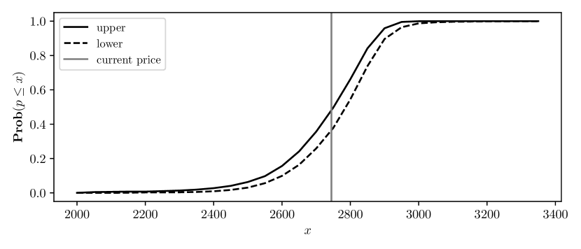
(a) Bounds on $\mathop{\bf Prob}(p\leq x)$.

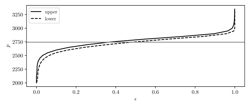
(b) Bounds on $\mathbf{VaR}(p,\epsilon)$.

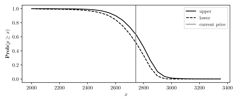
(c) Bounds on $\mathop{\bf Prob}(p\geq x)$.

Figure 2: SPX example. Bounds on CDF, $\mathbf{VaR}$, and CCDF.

Estimation.

We computed the maximum entropy risk-neutral distribution, as well as the (approximately) closest log-normal distribution to the set of risk-neutral probabilities. The closest log-normal distribution was $\log(p)\sim\mathcal{N}(7.917,0.05)$. Via Monte-Carlo simulation, we found that the annualized volatility of the index, assuming this log-normal distribution, was $19\%$, which is on par with SPX’s historical volatility of $15\%$. The resulting distributions are visualized in figure 3, and appear to be heavy-tailed to the left, meaning there is a large decrease in price is more probable than a large increase in price.

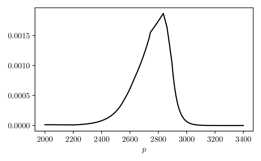
Figure 3: SPX example. Left: maximum entropy risk-neutral distribution; Right: closest log-normal distribution.

Bounds on costs.

We held out each put and call option one at a time and computed bounds on their bid and ask prices. In figure 4 we plot our computed lower and upper bounds along with the true prices. We observe that the bounds seem to be quite tight, and indeed bound the observed prices.

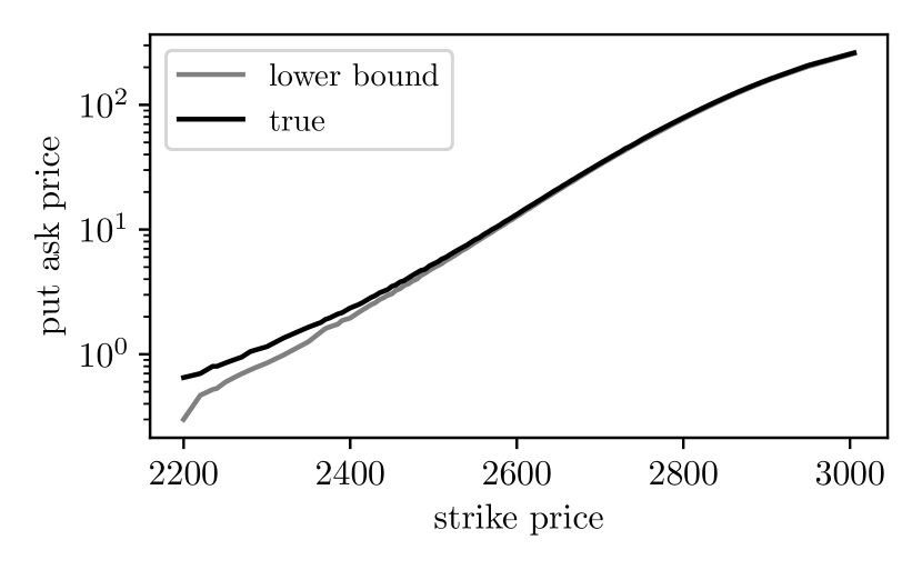
(a) Put ask prices.

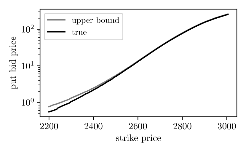
(b) Put bid prices.

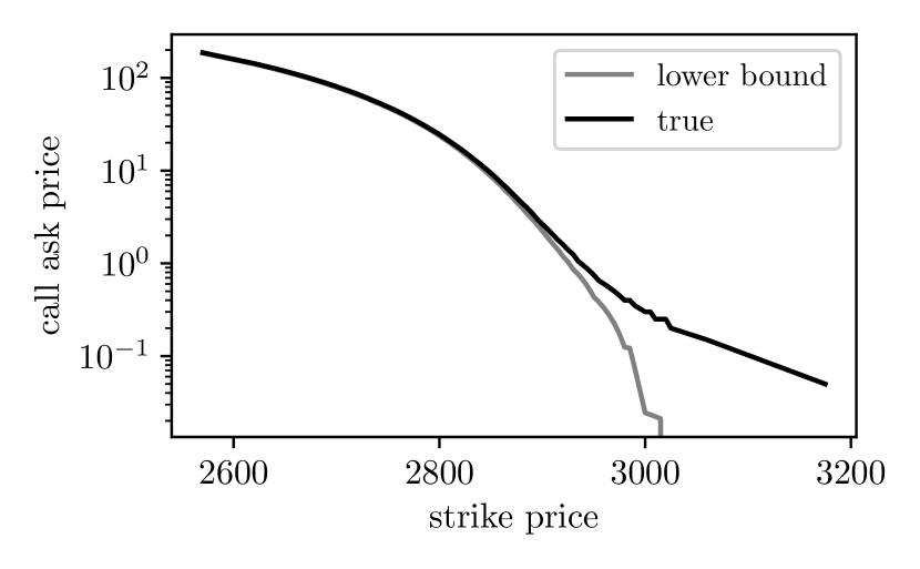
(c) Call ask prices.

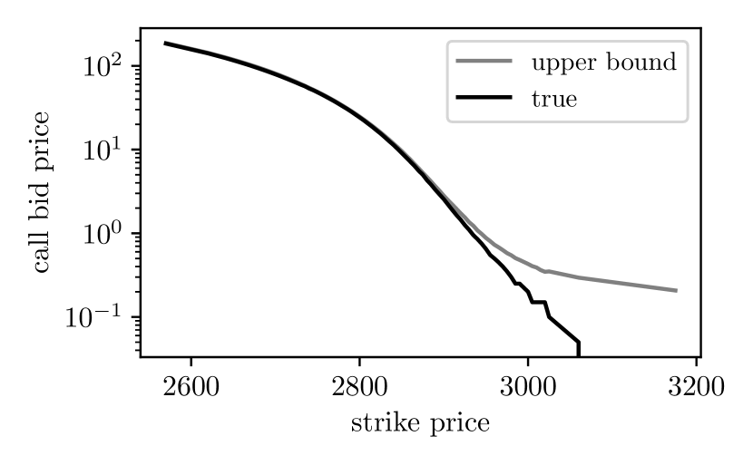
(d) Call bid prices.

Figure 4: SPX example. Bounds on costs.

4.2 Bitcoin

In our next example, we consider the crypto-currency Bitcoin as the underlying. As derivatives, we use Deribit European-style options and futures, whose underlying is the Deribit BTC index, which is the average of six leading BTC-USD exchange prices: Bitstamp, Bittrex, Coinbase Pro, Gemini, Itbit, and Kraken. We gathered the prices of March 27, 2020 Bitcoin options and futures on February 20, 2020 using the Deribit API [14].

We discretized the expiration price from 5 to 30000 dollars, in 5 dollar increments, resulting in $m=6000$ outcomes. We allow six possible investments: buying or selling puts, buying or selling calls, and buying or selling futures. The cost of each investment is the ask price if buying, the negative bid price if selling, plus a 0.04% fee for option transactions, a 0.075% fee for buying futures, and a 0.025% (market-maker) rebate for selling futures (which at the time of writing are the fees for the Deribit exchange).

In total, there were 16 puts and 19 calls expiring on March 27, with strike prices ranging from 4000 to 18000. This means there were $n=2(16+19)+2=72$ possible investments.

Functions of the price.

We calculated bounds on the expected value of the expiration price. The lower bound was 9847.7 dollars and the upper bound was 9852.57 dollars. We also computed bounds on the CDF, CCDF, and the value-at-risk of the expiration price. In figure 5 we plot these bounds.

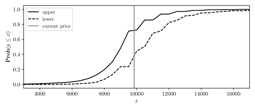
(a) Bounds on $\mathop{\bf Prob}(p\leq x)$.

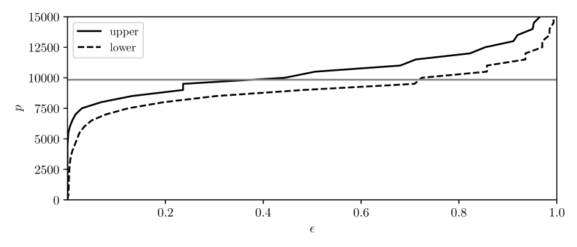
(b) Bounds on $\mathbf{VaR}(p,\epsilon)$.

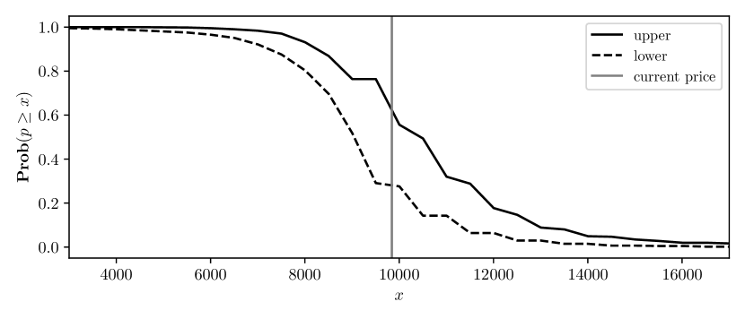
(c) Bounds on $\mathop{\bf Prob}(p\geq x)$.

Figure 5: Bitcoin example. Bounds on CDF, $\mathbf{VaR}$, and CCDF.

Estimation.

We computed the maximum entropy risk-neutral distribution, as well as the (approximately) closest log-normal distribution to the set of risk-neutral probabilities. The closest log-normal distribution was $\log(p)\sim\mathcal{N}(9.174,0.204)$. Via Monte-Carlo simulation, we found that the annualized volatility of the index, assuming this log-normal distribution, was $71.8\%$. The resulting distributions are visualized in figure 6, and appear to be heavy-tailed to the right, which is the opposite of the S&P 500 example.

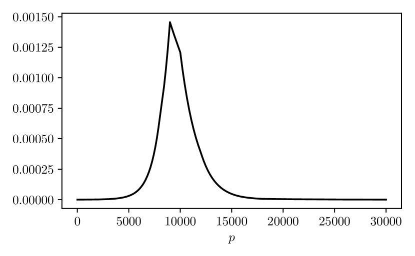
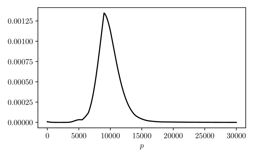
Figure 6: Bitcoin example. Left: maximum entropy risk-neutral distribution; Right: closest log-normal distribution.

Bounds on costs.

We held out each put and call option one at a time and computed bounds on their bid and ask prices. In figure 7 we plot our computed lower and upper bounds along with the true prices. We observe that the bounds are quite tight, and indeed bound the observed prices.

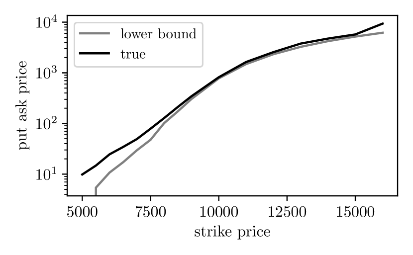
(a) Put ask prices.

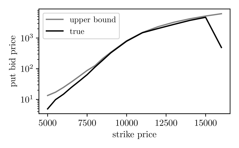
(b) Put bid prices.

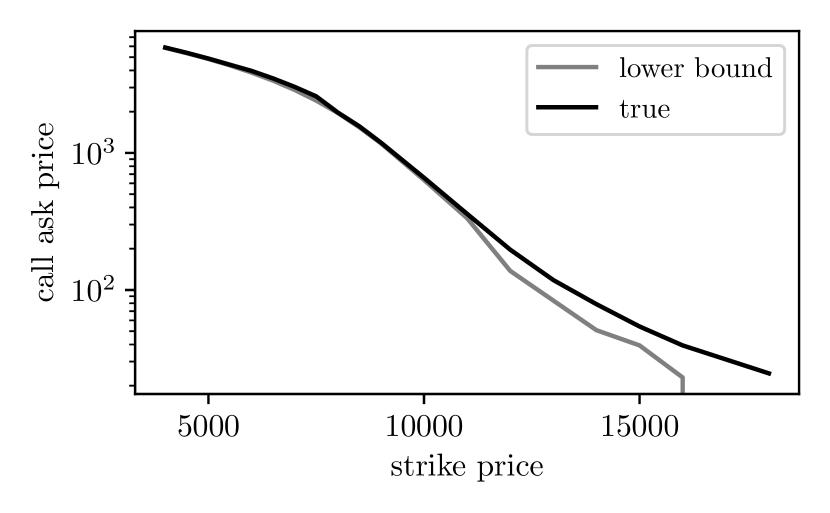
(c) Call ask prices.

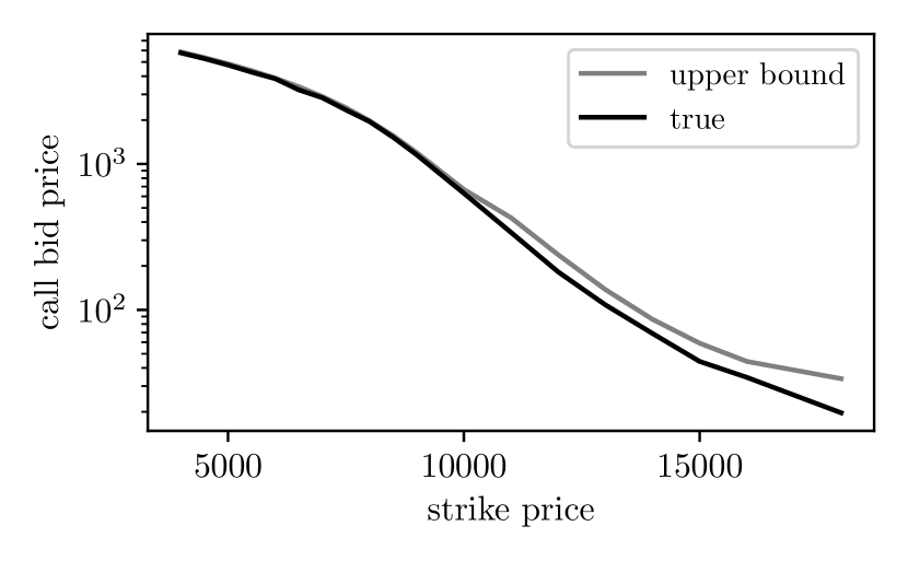
(d) Call bid prices.

Figure 7: Bitcoin example. Bounds on costs.

Sensitivities.

We computed the optimal dual variable of the constraint $P^{T}\pi\leq c$ for the entropy maximization problem. In table 1 we list the five largest dual variables, along with their corresponding investments and costs. We observe that shorting the underlying, as well as buying/writing various calls have the most effect on the maximum entropy risk-neutral probability. For example, if we decrease the price of the 9000 call by ten dollars, then the entropy will decrease by at least 0.01.

Table 1: Bitcoin example. Dual variables for entropy maximization problem.

Investment	$c_{i}$	$\lambda^{\star}_{i}$
Short underlying	-9847.65	0.001
Buy 9000 call	1191.268	0.001
Write 18000 call	-19.69	0.0004
Buy 10000 call	659.63	0.0004
Buy 8000 call	1973.96	0.0002

5 Conclusion

In this paper we described applications of minimizing a convex or quasiconvex function over the set of convex risk-neutral probabilities. These include computation of bounds on the cumulative distribution, VaR, conditional probabilities, and prices of new derivatives, as well as estimation problems. We reiterate that all of the aforementioned problems can be tractably solved, and due to DSLs, are easy to implement. A potential avenue for future research is use the set of risk-neutral probabilities for multiple expiration dates to somehow connect the distribution of the underlying’s price movements between those dates.

References

- [1] Wharton Research Data Services: OptionMetrics. https://wrds-www.wharton.upenn.edu/pages/about/data-vendors/optionmetrics/.
- [2] A. Agrawal, R. Verschueren, S. Diamond, and S. Boyd. A rewriting system for convex optimization problems. Journal of Control and Decision, 5(1):42–60, 2018.
- [3] J. Äijö. Impact of US and UK macroeconomic news announcements on the return distribution implied by FTSE-100 index options. International Review of Financial Analysis, 17(2):242–258, 2008.
- [4] Y. Aıt-Sahalia and A. Lo. Nonparametric risk management and implied risk aversion. Journal of Econometrics, 94(1-2):9–51, 2000.
- [5] D. Bates. Post-’87 crash fears in the S&P 500 futures option market. Journal of Econometrics, 94(1-2):181–238, 2000.
- [6] D. Bertsimas and I. Popescu. On the relation between option and stock prices: A convex optimization approach. Operations Research, 50(2):358–374, 2002.
- [7] D. Bertsimas and J. Tsitsiklis. Introduction to linear optimization. Athena Scientific, 1997.
- [8] F. Black and M. Scholes. The pricing of options and corporate liabilities. Journal of Political Economy, 81(3):637–654, 1973.
- [9] S. Boyd and L. Vandenberghe. Convex Optimization. Cambridge University Press, 2004.
- [10] N. Branger. Pricing derivative securities using cross-entropy: An economic analysis. International Journal of Theoretical and Applied Finance, 7(01):63–81, 2004.
- [11] P. Buchen and M. Kelly. The maximum entropy distribution of an asset inferred from option prices. The Journal of Financial and Quantitative Analysis, 31(1):143–159, 1996.
- [12] O. Castrén. Do options-implied RND functions on G3 currencies move around the times of interventions on the JPY/USD exchange rate? 2004.
- [13] G. Dantzig. Linear programming and extensions. Princeton University Press, 1998.
- [14] Deribit. Deribit API V2.0.0. https://docs.deribit.com/v2/#deribit-api-v2-0-0.
- [15] S. Diamond and S. Boyd. CVXPY: A Python-embedded modeling language for convex optimization. Journal of Machine Learning Research, 17(83):1–5, 2016.
- [16] D. Duffie. Dynamic asset pricing theory. Princeton University Press, 2010.
- [17] D. Duffie and J. Pan. An overview of value at risk. The Journal of Derivatives, 4(3):7–49, 1997.
- [18] J. Farkas. Theorie der einfachen ungleichungen. Journal fur die reine und angewandte Mathematik, 124:1–27, 1902.
- [19] A. Fu, B. Narasimhan, and S. Boyd. CVXR: An R package for disciplined convex optimization. In Journal of Statistical Software, 2019.
- [20] M. Grant and S. Boyd. Graph implementations for nonsmooth convex programs. In Recent Advances in Learning and Control, Lecture Notes in Control and Information Sciences, pages 95–110. Springer-Verlag Limited, 2008.
- [21] M. Grant and S. Boyd. CVX: Matlab software for disciplined convex programming, version 2.1, 2014.
- [22] J. Hull. Options, futures, and other derivatives. Pearson Prentice Hall, 2006.
- [23] J. Jackwerth. Generalized binomial trees. Journal of Derivatives, 5(2):7–17, 1996.
- [24] J. Jackwerth. Option-implied risk-neutral distributions and implied binomial trees: A literature review. The Journal of Derivatives, 7(2):66–82, 1999.
- [25] J. Jackwerth. Recovering risk aversion from option prices and realized returns. The Review of Financial Studies, 13(2):433–451, 2000.
- [26] J. Jackwerth. Option-implied risk-neutral distributions and risk aversion. 2004.
- [27] J. Jackwerth and M. Rubinstein. Recovering probability distributions from option prices. The Journal of Finance, 51(5):1611–1631, 1996.
- [28] W. Melick and C. Thomas. Recovering an asset’s implied PDF from option prices: an application to crude oil during the gulf crisis. Journal of Financial and Quantitative Analysis, 32(1):91–115, 1997.
- [29] R. Merton. Theory of rational option pricing. The Bell Journal of Economics and Management Science, pages 141–183, 1973.
- [30] T. Rockafellar and S. Uryasev. Optimization of conditional value-at-risk. Journal of Risk, 2:21–42, 2000.
- [31] S. Ross. Return, risk and arbitrage. Rodney L. White Center for Financial Research, The Wharton School, 1973.
- [32] M. Rubenstein. Implied binomial trees. The Journal of Finance, 49(3):771–818, 1994.
- [33] M. Stutzer. A simple nonparametric approach to derivative security valuation. The Journal of Finance, 51(5):1633–1652, 1996.
- [34] M. Udell, K. Mohan, D. Zeng, J. Hong, S. Diamond, and S. Boyd. Convex optimization in Julia. Workshop on High Performance Technical Computing in Dynamic Languages, 2014.