General description for nonequilibrium steady states
in periodically driven dissipative quantum systems

Abstract

Laser technology has developed and accelerated photo-induced nonequilibrium physics from both scientific and engineering viewpoints. The Floquet engineering, i.e., controlling material properties and functionalities by time-periodic drives, is a forefront of quantum physics of light-matter interaction, but limited to ideal dissipationless systems. For the Floquet engineering extended to a variety of materials, it is vital to understand the quantum states emerging in a balance of the periodic drive and energy dissipation. Here we derive the general description for nonequilibrium steady states (NESS) in periodically driven dissipative systems by focusing on the systems under high-frequency drive and time-independent Lindblad-type dissipation with the detailed balance condition. Our formula correctly describes the time-average, fluctuation, and symmetry property of the NESS, and can be computed efficiently in numerical calculations. Our approach will play fundamental roles in Floquet engineering in a broad class of dissipative quantum systems such as atoms and molecules, mesoscopic systems, and condensed matters.

I Introduction

State-of-the-art laser technology has opened new research fields in physics: the Floquet science and engineering Holthaus (2015); Bukov et al. (2015); Oka and Kitamura (2019). The main focus of these fields is the nonequilibrium states driven periodically by external fields, e.g., intense laser fields. Physical properties of the nonequilibrium states are mainly understood by the so-called effective Hamiltonian, which reflects the periodic driving, according to the Floquet theorem Shirley (1965) and the ensuing theoretical developments Eckardt and Anisimovas (2015); Mikami et al. (2016); Lazarides et al. (2014); Kuwahara et al. (2016). Conversely, designing a suitable driving protocol, one can engineer the effective Hamiltonian, which enables us to have desirable properties and functionalities of physical systems. Indeed, various exotic states and useful manipulation of matter have been theoretically proposed and some of them have been experimentally realized: Floquet topological states Oka and Aoki (2009) in solids Wang et al. (2013), ultracold atomic gases Jotzu et al. (2014), and in photonic wave guides Rechtsman et al. (2013), Floquet time crystals Else et al. (2016) in nitrogen-vacancy centers Choi et al. (2017) and trapped ions Zhang et al. (2017), and control of quantum magnets Sato et al. (2016) and their interactions Mentink et al. (2015).

However, these Floquet-theoretical predictions based on the effective Hamiltonian are quantitatively only in ultraclean materials or well-designed artificial systems, where dissipation is negligible. For the Floquet science and engineering in real generic materials, it is indispensable to understand the nonequilibrium steady state (NESS), which emerges in a balance of the energy injection by the periodic driving and the energy dissipation Kohn (2001); Hone et al. (2009); Kohler et al. (1997); Breuer et al. (2000). For individual systems, by considering specific sources of dissipation i.e. system-bath couplings, one can calculate physical quantities in the NESS and predict interesting phenomena such as Floquet topological insulators Dehghani et al. (2014); Seetharam et al. (2015), periodic thermodynamics Schmidt et al. (2019), dynamical localization Blümel et al. (1991), and generalized Bose-Einstein condensation Vorberg et al. (2013). In this research direction, the Floquet-Green-function approach has developed and enables us to calculate various physical effects dependent on the type of the system-bath coupling Kohler et al. (2004); Stefanucci et al. (2008). Another research direction, which we address here, is to seek for a universal characterization for the NESS. We could imagine that there exists a simple and general expression for the NESS when the dissipation is weak and featureless. An attempt is to conjecture that the NESS is generally described by the Floquet-Gibbs state (FGS), i.e., the Gibbs state with the effective Hamiltonian, but the conditions for the FGS being realized have shown quite restrictive Shirai et al. (2015, 2016); Liu (2015). Hence, despite its importance, the general formula for the NESS has been still an elusive problem.

In this paper, in exchange for restricting ourselves to the high-frequency drivings, we deal with generic systems and driving protocols, obtaining simple and general formulas for the NESS [Eqs. (7)–(10) below]. We obtain these formulas by applying the high-frequency expansion technique, which has been recently developed Goldman and Dalibard (2014); Rahav et al. (2003); Eckardt and Anisimovas (2015); Mikami et al. (2016); Dai et al. (2016), to the Lindblad equation with periodic Hamiltonians. As exemplified in an effective model for the NV center in diamonds Rondin et al. (2014), our formulas correctly describe both the time average and fluctuation of the NESS at the leading order of $\omega^{-1}$ ($\omega$ denotes the driving frequency). These formulas also capture nontrivial behaviors of physical quantities due to the dynamical-symmetry breaking that cannot be described by the effective Hamiltonian or the FGS, and will thereby play critical roles in the Floquet science and engineering in dissipative quantum systems.

II Formulation of the problem

We begin by considering a quantum system defined on an $N$-dimensional Hilbert space. This system can be single-body or many-body as long as it satisfies the requirements that will be described below. We let $H_{0}$ denote the time-independent Hamiltonian, which describes our system in the absence of driving. The eigenenergies and eigenstates of $H_{0}$ are denoted by $\{E_{i}\}_{i=1}^{N}$ and $\{\ket{E_{i}}\}_{i=1}^{N}$, respectively. For simplicity, we assume that the eigenenergies are not degenerate and $E_{1}<E_{2}<\cdots<E_{N}$ (the generalization to degenerate $H_{0}$ is formulated in Supplemental Material). The effect of the driving is represented by a time-dependent part $H_{\text{ext}}(t)$ of the total Hamiltonian,

$$H(t)=H_{0}+H_{\text{ext}}(t).$$ (1)

We assume that the driving term is periodic with period $T$: $H_{\text{ext}}(t+T)=H_{\text{ext}}(t)$ and hence $H(t+T)=H(t)$. Without loss of generality, the decomposition (1) is defined so that the time average of $H_{\text{ext}}(t)$ vanishes, $\int_{0}^{T}dt\ H_{\text{ext}}(t)=0$. Thus the Fourier series of $H_{\text{ext}}(t)$ can be written as

$$H_{\text{ext}}(t)=\sum_{m\neq 0}{H}_{m}e^{-im\omega t}.$$ (2)

To study driven dissipative systems, we consider the density operator $\rho(t)$ whose dynamics is described by the Lindblad equation Ho et al. (1986); Prosen and Ilievski (2011); Hartmann et al. (2017); Breuer and Petruccione (2002) (we set $\hbar=1$ throughout this paper):

$$\frac{d\rho(t)}{dt} =\mathcal{L}_{t}\rho(t)=-i\left[H(t),\rho(t)\right]+\mathcal{D}[\rho(t)],$$

$$\mathcal{D}[\rho(t)] \equiv\sum_{i,j}\Gamma_{ij}\left(L_{ij}\rho(t)L_{ij}^{\dagger}-\frac{1}{2}\left\{L_{ij}^{\dagger}L_{ij},\rho(t)\right\}\right).$$ (3)

Here $L_{ij}:=\ket{E_{i}}\bra{E_{j}}$ is the time-independent Lindblad operator describing the transition from the $j$-th to the $i$-th eigenstates of the undriven Hamiltonian $H_{0}$. When $E_{i}<E_{j}$, $L_{ij}$ represents a decay (excitation) process for $i<j$ ($i>j$). The real number $\Gamma_{ij}$ $(\geq 0)$ denotes the rate for the corresponding process, and we set $\Gamma_{ii}=0$ for each $i$. The transition rates $\Gamma_{ij}$ must be small enough for the Floquet-Lindblad equation being valid (see Discussion below). Note that Eq. (II) is trace-preserving $d\,\text{tr}[\rho(t)]/dt=0$, and thus we use the normalization $\mathrm{tr}[\rho(t)]=1$.

We assume that the transition rates $\Gamma_{ij}$ satisfy the detailed balance condition,

$$\Gamma_{ij}e^{-\beta E_{j}}=\Gamma_{ji}e^{-\beta E_{i}}\qquad(\text{for}\ i\neq j),$$ (4)

where $\beta$ is the inverse temperature of the bath coupled to the system (see Discussion below for generalization in the absence of this assumption). We also assume that the matrix $\Gamma_{ij}$ is a nonnegative irreducible matrix Schmidt (2020). These assumptions ensure that, without driving, the system goes, irrespective of the initial state, to the thermal equilibrium state, or the canonical ensemble $\rho_{\text{can}}=e^{-\beta H_{0}}/Z$ of $H_{0}$ with $Z=\text{tr}(e^{-\beta H_{0}})$. We note that the Lindblad operators $L_{ij}$ may depend on the driving in general if we consider more microscopic theories of dissipation Breuer et al. (2000). However, we neglect this dependence in this work for simplicity.

III Derivation of main results by high-frequency expansion

The key idea to obtain the nonequilibrium steady state is the high-frequency expansion for the Lindblad equation Dai et al. (2016). Among several formulations, we adopt the van Vleck perturbation theory Eckardt and Anisimovas (2015); Mikami et al. (2016), which leads to the following propagation for $\rho(t)$ (see Supplementary Material for detail): $\rho(t)=e^{\mathcal{G}(t)}e^{(t-t^{\prime})\mathcal{L}_{\text{eff}}}e^{-\mathcal{G}(t^{\prime})}\rho(t^{\prime})$. The time-independent part $\mathcal{L}_{\text{eff}}$ is represented by the effective Hamiltonian

$$\mathcal{L}_{\text{eff}}(\rho)=-i[{H}_{\mathrm{eff}},\rho]+\mathcal{D}(\rho)+O(\omega^{-2})$$ (5)

with ${H}_{\mathrm{eff}}=H_{0}+\omega^{-1}\sum_{n>0}[{H}_{-n},{H}_{n}]/n+O(\omega^{-2})$. The time-dependent part $e^{\mathcal{G}(t)}$ is the so-called micromotion operator periodic in time $\mathcal{G}(t+T)=\mathcal{G}(t)$, and given by $\mathcal{G}(t)(\rho)=\omega^{-1}\sum_{m\neq 0}[{H}_{m},\rho]e^{-im\omega t}/m+O(\omega^{-2})$. Without loss of generality, we suppose the initial time to be $t^{\prime}=0$, having

$$\rho(t)=e^{\mathcal{G}(t)}e^{t\mathcal{L}_{\text{eff}}}e^{-\mathcal{G}(0)}\rho(0)$$ (6)

with $\rho(0)$ being our initial state.

To obtain the asymptotic behavior of $\rho(t)$, we focus on the first part $\rho^{\prime}(t)=e^{t\mathcal{L}_{\text{eff}}}e^{-\mathcal{G}(0)}\rho(0)$. Remark that this is the solution of the time-independent Lindblad equation $d\rho^{\prime}(t)/dt=\mathcal{L}_{\text{eff}}\rho^{\prime}(t)$ from the initial state $e^{-\mathcal{G}(0)}\rho(0)$. Under our assumptions on $\mathcal{D}$, $\rho^{\prime}(t)$ approaches, irrespective of the initial state, the unique state ${\rho}^{\prime}_{\infty}$ characterized by $\mathcal{L}_{\text{eff}}{\rho}^{\prime}_{\infty}=0$.Thus we come to the first main result, obtaining the asymptotic behavior

$$\rho(t)\to{\rho}_{\text{ness}}(t)=e^{\mathcal{G}(t)}{\rho}^{\prime}_{\infty}\qquad\text{as}\quad t\to\infty.$$ (7)

Since $\mathcal{G}(t)=\mathcal{G}(t+T)$, this nonequilibrium steady state is also periodic in time. Focusing on the leading-order contribution, we have a simple explicit formula for ${\rho}_{\text{ness}}(t)$:

$${\rho}_{\text{ness}}(t)=\rho_{\text{can}}+{\sigma}_{\text{MM}}(t)+{\sigma}_{\text{FE}}+O(\omega^{-2}),$$ (8)

in which both ${\sigma}_{\text{MM}}(t)$ and ${\sigma}_{\text{FE}}$ are $O(\omega^{-1})$ and we call ${\sigma}_{\text{MM}}(t)$ and ${\sigma}_{\text{FE}}$ the micromotion and Floquet engineering parts, respectively. Equation (8) is our second main result, which we prove in the Supplemental Material. Its generalization in the absence of the detailed balance condition is outlined in Discussion below. Note that $\text{tr}[{\rho}_{\text{ness}}(t)]=1$ is satisfied, at least, up to this order since both ${\sigma}_{\text{MM}}(t)$ and ${\sigma}_{\text{FE}}$ are traceless as will be evident below.

The micromotion part ${\sigma}_{\text{MM}}(t)$ in Eq. (8) is defined by

$${\sigma}_{\text{MM}}(t)=\frac{1}{\omega}\sum_{m\neq 0}\frac{e^{-im\omega t}}{m}[H_{m},\rho_{\text{can}}].$$ (9)

We have named it after the following two properties of ${\sigma}_{\text{MM}}(t)$. First, this part is periodic in time ${\sigma}_{\text{MM}}(t+T)={\sigma}_{\text{MM}}(t)$ and contributes to oscillations of physical observables. Second, ${\sigma}_{\text{MM}}(t)$ does not contribute to the time averages of physical observables for one period of oscillations. In fact, for an observable ${A}$, we have $\int_{t_{1}}^{t_{1}+T}dt\,\text{tr}[{\sigma}_{\text{MM}}(t){A}]/T=0$.

The Floquet-engineering part ${\sigma}_{\text{FE}}$ in Eq. (8) is independent of time and given by

$$\braket{E_{k}}{{\sigma}_{\text{FE}}}{E_{l}}=\frac{\braket{E_{k}}{\varDelta{H}_{\mathrm{eff}}}{E_{l}}}{(E_{k}-E_{l})-i\gamma_{kl}}(p_{\text{can}}^{(k)}-p_{\text{can}}^{(l)})$$ (10)

for $k\neq l$ and $\braket{E_{k}}{{\sigma}_{\text{FE}}}{E_{k}}=0$ for all $k$, where $\varDelta{H}_{\mathrm{eff}}\equiv{H}_{\mathrm{eff}}-H_{0}=O(\omega^{-1})$, $p_{\text{can}}^{(k)}=e^{-\beta E_{k}}/Z$ is the Boltzmann weight, and $\gamma_{kl}\equiv\sum_{i}(\Gamma_{ik}+\Gamma_{il})/2$ represents the symmetric decay-rate matrix (see Supplemental Material for the generalization to degenerate $H_{0}$). We call ${\sigma}_{\text{FE}}$ the Floquet engineering part because it describes how the effective Hamiltonian changes physical observables from their values in thermal equilibrium. In contrast to the micromotion part, the Floquet engineering part contributes to the time-averaged quantities. As discussed below, Eq. (4) is regular in the weak dissipation limit $\gamma_{ij}\to 0$, where we obtain ${\sigma}_{\text{FE}}$ and hence $\rho_{\mathrm{ness}}(t)$ independent of $\gamma_{ij}$, and $\rho_{\mathrm{ness}}(t)$ coincides with the canonical Floquet steady state that we define.

Equation (10) serves as the foundation for the Floquet engineering in dissipative quantum systems. Let us imagine, for example, that an observable ${A}$ has zero expectation value at thermal equilibrium, $\text{tr}(\rho_{\text{can}}{A})=0$, but nonzero value for the NESS, $\text{tr}({\sigma}_{\text{FE}}{A})\neq 0$. This situation means that one can implement an appropriate periodic driving $H_{\text{ext}}(t)$ and hence $\varDelta{H}_{\mathrm{eff}}$, thereby activating the observable ${A}$. Upon this engineering, Eq. (10) tells us how much activation is possible for observables of interest. We will see some examples below.

In addition to their generality, our formulas [Eqs. (8)–(10)] are extremely efficient in practical calculations of the nonequilibrium steady state. In the straightforward calculation, one numerically integrates the time-dependent Lindblad equation (II) with a sufficiently small time step until the system reaches the NESS. In contrast, our formulas enable us to evaluate the NESS at an arbitrary time $t$ without numerical integration once we have the energy eigenstates $\{\ket{E_{k}}\}$ of the time-independent Hamiltonian $H_{0}$. This difference of efficiency becomes more evident when the Hilbert-space dimension $N$ is large. In the straightforward calculation, the density matrix $\rho(t)$ is commonly treated as an $N^{2}$-dimensional vector and the superoperator $\mathcal{L}_{t}$ as an $N^{2}\times N^{2}$ matrix. Thus the computational complexity for each time step is $O(N^{4})$ in general. On the other hand, the complexity for our formula is one-order smaller and given by , which derives from the exact diagonalization of $O(N^{3})$. Thus our formulas enable us to evaluate the NESS for larger Hilbert-space dimensions that occur, for example, in quantum many-body systems. For special cases where $\mathcal{L}_{t}$ is a sparse matrix and has only $O(N^{0})$ nonzero elements, the computational complexity for one time step is $O(N^{2})$. Nevertheless, even for these cases, we need many time steps typically larger than $N$, in obtaining accurate results and, hence, our formulas require less computational complexity.

IV Numerical verification in a single spin with $S=1$

By taking a single spin with $S=1$, we demonstrate how our formula (8) works in the quantum dynamics described by the Lindblad equation (II). We consider an effective Hamiltonian for the NV center in diamonds Rondin et al. (2014):

$${H}_{\text{NV}}(t) =-B_{s}S_{z}+\mathcal{N}_{z}S_{z}^{2}+\mathcal{N}_{xy}(S_{x}^{2}-S_{y}^{2})+H_{\text{ext}}^{\text{circ}}(t),$$ (11)

where $B_{s}$ is the static Zeeman field, $\mathcal{N}_{z}$ and $\mathcal{N}_{xy}$ are the coupling constants of magnetic anisotropic terms, and $H_{\text{ext}}^{\text{circ}}(t)\equiv-B_{d}(S_{x}\cos\omega t+S_{y}\sin\omega t)$ represents the coupling to the circularly-polarized ac magnetic field. We note that the energy eigenstates of the time-independent part of Eq. (11) are analytically obtained and our formula can be computed almost analytically in this model. Since $\mathcal{N}_{z}\gg\mathcal{N}_{xy}$ in the NV centers Rondin et al. (2014), we set $\mathcal{N}_{z}=1$ and $\mathcal{N}_{xy}=0.05$ in our analysis.

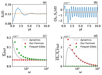
Figure 1: (Top) Time evolution of (a) $S_{z}$ and (b) $\{S_{x},S_{y}\}=S_{x}S_{y}+S_{y}S_{x}$ of a single spin described by the Lindblad equation (II) with the Hamiltonian (11) (see text for the parameters). The dashed line show the one-cycle average at a sufficiently long time. (Bottom) One-cycle average $\bar{A}(\omega)$ for (c) ${A}=S_{z}$ and (d) ${A}=\{S_{x},S_{y}\}$ calculated from the dynamics simulation (solid line), our formula [Eq. (8)] (circle), and the FGS [Eq. (12)] (square). All the other parameters except $\omega$ are the same as in the top panels.

Typical time evolutions $O(t)\equiv\mathrm{tr}[\rho(t){A}]$ are shown for two representative observables ${A}=S_{z}$ and $\{S_{x},S_{y}\}$ $(=S_{x}S_{y}+S_{y}S_{x})$ in Figs. 1(a) and (b), respectively. In this calculation, we take the thermal state for the time-independent part of ${H}_{\text{NV}}$ at $t=0$, and let it evolve according to the Lindblad equation (II) with $H(t)$ being ${H}_{\text{NV}}(t)$. The static Zeeman field is $B_{s}=0.3$, and the driving parameters are $B_{d}=0.1$ and $\omega=1$. As for the Lindblad operators, we take $\Gamma_{ij}$ according to the heatbath method as $\Gamma_{ij}=\gamma e^{-\beta E_{i}}/(e^{-\beta E_{i}}+e^{-\beta E_{j}})$ for $i\neq j$ with rate constant $\gamma=0.2$ and $\beta=3$, and $\Gamma_{ii}=0$ for all $i$’s. Figures 1(a) and (b) show that, after a sufficiently long time $t\gg\gamma^{-1}$, the system reaches the nonequilibrium steady state, in which the observables oscillate with period $T=2\pi/\omega$. In particular, the observable ${A}=\{S_{x},S_{y}\}$ is initially zero for a symmetry reason (e.g., $S_{x}\to-S_{x}$), but becomes nonzero on time average. Namely, this observable is engineered by the periodic drive $H_{\text{ext}}^{\text{circ}}(t)$.

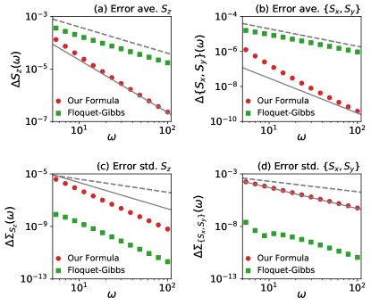
Figure 2: (Top) Difference $\Delta{A}(\omega)$ between the one-cycle average $\bar{A}(\omega)$ calculated from the dynamics simulation and that from our formula [Eq. (8)] (circle) or the FGS [Eq. (12)] (square) plotted against $\omega$ for (a) ${A}=S_{z}$ and (b) ${A}=\{S_{x},S_{y}\}$. (Bottom) Difference $\Delta{\Sigma_{A}}(\omega)$ between the one-cycle standard deviation $\Sigma_{A}(\omega)$ calculated from the dynamics simulation and that from our formula [Eq. (8)] (circle) or the FGS [Eq. (12)] (square) plotted against $\omega$ for (c) ${A}=S_{z}$ and (d) ${A}=\{S_{x},S_{y}\}$. In all the panels, the solid and dashed lines are guides for the eye, showing $\propto\omega^{-2}$ and $\propto\omega^{-1}$, respectively.

To test our formula (8) quantitatively, we first focus on the one-cycle average $\bar{A}(\omega)=T^{-1}\int_{t}^{t+T}ds\,\mathrm{tr}[\rho(s){A}]$ for $t\gg\gamma^{-1}$. In Figs. 1(c) and (d), we compare the one-cycle averages calculated from the actual dynamics and those calculated from our formulas (8) and (10) (recall that the micromotion part ${\sigma}_{\text{MM}}(t)$ does not contribute to the one-cycle averages). At high frequency $\omega\gtrsim 10$, the difference of the actual dynamics and our formula decreases quite well. Defining this difference as $\Delta A(\omega)$, we plot it against $\omega$ for ${A}=S_{z}$ and $\{S_{x},S_{y}\}$ in Figs. 2(a) and (b), respectively. We stress that the difference $\Delta A(\omega)$ decreases more rapidly than $O(\omega^{-1})$ ($O(\omega^{-2})$ for $S_{z}$ and $O(\omega^{-3})$ for $\{S_{x},S_{y}\}$). This means that our formulas (8) and (10) perfectly describe the actual NESS at the level of $O(\omega^{-1})$. As shown in Supplemental Material, $\Delta A(\omega)=O(\omega^{-2})$ holds true not only for the two observables but also for all the other observables. Therefore, we have verified our formula (8) apart from the micromotion part.

For the complementary test of our formula (8), we consider the one-cycle standard deviation $\Sigma_{A}(\omega)=\{T^{-1}\int_{t}^{t+T}ds\,\{\mathrm{tr}[\rho(s){A}]-\bar{A}(\omega)\}^{2}\}^{1/2}$, which quantifies the micromotion amplitude. This quantity is suitable for testing our formula (8) because it is contributed only by the micromotion part ${\sigma}_{\text{MM}}(t)$. Since $\Sigma_{A}(\omega)$ is an $O(\omega^{-1})$ quantity in general, the accuracy of our formula is verified if the difference $\Delta\Sigma_{A}(\omega)$ is $O(\omega^{-2})$, where $\Delta\Sigma_{A}(\omega)$ is defined by (the absolute value of) the difference between $\Sigma_{A}(\omega)$ calculated from the actual dynamics and that from our formulas (8) and (9). This criterion is indeed satisfied as shown in Figs. 2(c) and (d) for ${A}=S_{z}$ and $\{S_{x},S_{y}\}$, respectively. We remark that our formula leads to $\Sigma_{A}(\omega)=0$ at $O(\omega^{-1})$ for these observables, which can be analytically shown by noticing ${H}_{\pm 1}\propto{S}_{\pm}=S_{x}\pm iS_{y}$. Thus the plotted data correspond to $\Sigma_{A}(\omega)$ itself for the actual dynamics, and $\Delta\Sigma_{A}(\omega)$ could be reduced by dealing with the higher-order terms in Eq. (8). In any case, the fact that $\Delta\Sigma_{A}(\omega)=O(\omega^{-2})$ justifies our formulas (8) and (9).

V Comparison with the Floquet-Gibbs state

Let us make comparisons with the Floquet-Gibbs state (FGS), which has been a candidate for the ensemble description of the periodically driven dissipative quantum systems Shirai et al. (2015, 2016); Liu (2015). To define the FGS, we introduce the Floquet state $\ket{u_{i}(t)}$ and its quasienergy $\epsilon_{i}$. According to the Floquet theorem, the time-dependent Schrödinger equation $i\frac{d}{dt}\ket{\psi(t)}=H(t)\ket{\psi(t)}$ has the independent solutions $\ket{\psi_{i}(t)}=e^{-i\epsilon_{i}t}\ket{u_{i}(t)}$ $(i=1,2,\dots,N)$ with periodicity $\ket{u_{i}(t+T)}=\ket{u_{i}(t)}$. In terms of the Floquet states, the FGS is defined by

$${\rho}_{\text{FG}}(t)=\frac{1}{Z_{\text{FG}}}\sum_{i}e^{-\beta\epsilon_{i}}\ket{u_{i}(t)}\bra{u_{i}(t)},$$ (12)

where $Z_{\text{FG}}=\sum_{i}e^{-\beta\epsilon_{i}}$. To obtain the Floquet states and quasienergies in practice, the common method, which we employ here, is to calculate the one-cycle unitary evolution ${U}(T)=\mathbb{T}\exp[-i\int_{0}^{T}ds\,H(s)]$, where $\mathbb{T}$ denotes the time-ordered exponential, by numerical integrations of the time-dependent Schrödinger equation. The eigenvectors and eigenvalues of ${U}(T)$ correspond to $\ket{u_{i}(0)}$ and $e^{-i\epsilon_{i}T}$, which give us $\epsilon_{i}$ and $\ket{u_{i}(t)}$. Note that the Floquet states and quasienergies thus obtained are exact and involve all-order contributions in $1/\omega$.

Quantitative comparisons between the actual dynamics and FGS are shown in Fig. 2. In panel (a) and (d), we plot the difference of the one-cycle average calculated from the actual dynamics and FGS for the two representative observables ${A}=S_{z}$ and $\{S_{x},S_{y}\}$. Remarkably, the difference is $O(\omega^{-1})$, meaning that the FGS cannot reproduce the leading-order contribution of the one-cycle average  in contrast to our formula (8). As for the micromotion amplitude, or the one-cycle standard deviation $\Sigma_{A}(\omega)$, the FGS reproduce the actual values better than our formulas (8) and (9). This is partly because the FGS involve all-order contributions in $1/\omega$ while our formulas are the leading-order approximation. As stated above, our formula could be improved order-by-order when we start over from our first main result (7).

A weak point of the FGS is highlighted in Fig. 1(d), in which the FGS gives $\overline{\{S_{x},S_{y}\}}(\omega)=0$ for any $\omega$ while it is not true in the actual dynamics. This is due to an antiunitary dynamical symmetry constraining the Floquet states and hence the FGS. In fact, we take an antiunitary operator ${V}$: ${V}S_{y}{V}^{\dagger}=-S_{y}$ and ${V}{S}_{\alpha}{V}^{\dagger}={S}_{\alpha}$ ($\alpha=x$ and $z$). Then we notice the dynamical symmetry ${V}{H}_{\text{NV}}(T-t){V}^{\dagger}={H}_{\text{NV}}(t)$, which implies that $\ket{\tilde{u}_{i}(t)}\equiv{V}\ket{u_{i}(T-t)}$ is also a Floquet state with quasienergy $\epsilon_{i}$. Assuming that quasienergies are not degenerate as in our examples, we have that $\ket{\tilde{u}_{i}(t)}$ and $\ket{u_{i}(t)}$ are equivalent up to an overall phase shift. Owing to ${V}{A}{V}^{\dagger}=-{A}$ with ${A}=\{S_{x},S_{y}\}$, the one-cycle averages of ${A}$ calculated for $\ket{\tilde{u}_{i}(t)}$ and $\ket{u_{i}(t)}$ differ by their signs, meaning that the one-cycle average vanishes in fact. Note that similar arguments apply to other observables satisfying ${V}{A}{V}^{\dagger}=-{A}$.

We remark that the dissipation can break such an antiunitary dynamical symmetry and this is the origin of the nonzero one-cycle average of $\overline{\{S_{x},S_{y}\}}(\omega)$. We can show that this average vanishes by taking the limit $\gamma_{ij}\to 0$ in Eq. (10). In other words, the NESS in dissipative systems shows richer properties inferred only from the effective Hamiltonian itself. Our formula (8) well describes these properties unlike the FGS (12), which incorporates no information about the dissipation, or the Lindblad operators.

One might be interested in an approximate description of the NESS independent of the details of $\gamma_{ij}$ for weak dissipation, and expect that the FGS serves as such a description. Interestingly, this is not true at least within our formulation of periodically driven dissipative systems described by Eqs. (II) and (4). Instead, the actual NESS coincides with yet another state which we name the canonical Floquet steady state (CFSS) defined by replacing the quasienergy $\epsilon_{i}$ by the real energy $E_{i}$ in Eq. (12). One can show this by comparing the high-frequency expansion of the CFSS and our formulas [Eqs. (7)–(10)] in the limit of $\gamma_{ij}\to 0$ (see Supplemental Material for details).

VI Discussions and Conclusions

We have derived and verified the simple and general formulas [Eqs. (7)–(10)] describing the NESS in dissipative quantum systems under high-frequency periodic drivings. We have also exemplified the dynamical symmetry breaking and the possibility of the Floquet engineering in driven dissipative systems in the NV centers in diamonds. Being quite general, our formulas would play the fundamental role in understanding and engineering unusual nonequilibrium states in various quantum systems such as atoms and molecules, trapped ions, condensed matters, and so on.

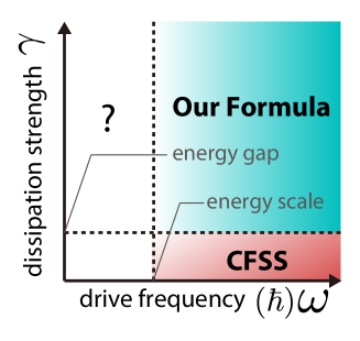
Figure 3: Validity of NESS formulas in parameter space. Our formula is valid when the driving frequency $\omega$ is larger than energy scales of the system. When the dissipation strength is smaller than the (nonzero) minimum energy gap, our formula reduces to the CFSS. At lower frequency, the NESS description remains an open question.

The parameter region in which our formulas are valid is depicted in Fig. 3. Based on the high-frequency expansion, our formulas are valid when the driving frequency $\omega$ (more precisely, the photon energy $\hbar\omega$) is greater than the energy scales of the system and the system-drive coupling. We note, however, that our formulas hold true for any strength of dissipation $\Gamma_{ij}$ (or $\gamma_{ij}$) within the Floquet-Lindblad equation (II). As we have shown, our formulas reduce to the CFSS rather than the FGS when the dissipation strength is smaller than the energy gap, i.e., the nonzero minimum difference between eigenenergies (our formulas are generalized for the degenerate Hamiltonian in Supplementary Materials).

One should note that the Floquet-Lindblad equation (II) becomes invalid when $\Gamma_{ij}$ is too large. The Lindblad-type dissipation is derived from several approximations such as the Born-Markov approximation Breuer and Petruccione (2002). These approximations require the condition that the relaxation time $\sim 1/\Gamma_{ij}$ is longer than the time scale of system’s dynamics and the bath correlation time. Namely, the dissipation rate $\Gamma_{ij}$ should be smaller than the other relevant energy scales. Note that the high-frequency driving does not break this condition while lower frequencies may be problematic.

We remark a further generalization of our results Eqs. (7)–(10). Although we have assumed the detailed balance condition (4), this condition can be removed as long as the transition-rate matrix $\Gamma_{ij}$ is irreducible. In this case, the solution of the Lindblad equation without driving is not the canonical ensemble $\hat{\rho}_{\text{can}}$ but another state $\tilde{\rho}$ characterized by $-i[H_{0},\tilde{\rho}]+\mathcal{D}(\tilde{\rho})=0$. Correspondingly, our results for the NESS [Eqs. (7)–(10)] hold true with the following replacements: $\hat{\rho}_{\text{can}}\to\tilde{\rho}$ and $p_{\text{can}}^{(k)}\to\tilde{p}_{\text{can}}^{(k)}=\braket{E_{k}}{\tilde{\rho}}{E_{k}}$. Thus our formulas apply to any periodically driven dissipative systems as long as the dissipation is of Lindblad type and irreducible. Therefore, our formulas are useful for a broad class of systems in exploring generic features of the NESS and in estimating Floquet-engineered physical quantities.

It remains an open question to find a simple and general formula for the NESS at lower frequency. The applicability of the CFSS in many-body systems is also a nontrivial issue because the energy gap can be very small in those systems. Addressing these issues will lead us to the complete understanding of the NESS in dissipative Floquet systems.

S1 High-frequency expansion for the Lindblad equation

The high-frequency expansion has been developed in unitary dynamics and there are several formulations as summarized in Ref. Mikami et al. (2016). For the Lindblad equation, the high-frequency expansion has been discussed in terms of the Floquet-Magnus formalism in Ref. Dai et al. (2016). In this paper, we make use of the high-frequency expansion of the Lindblad equation in terms of the van Vleck approach, which we describe below for completeness.

The Lindblad equation that we discuss in this work is symbolically represented as

$$\partial_{t}\hat{\rho}(t)=\mathcal{L}(t)\hat{\rho}(t),$$ (S1)

where the time-dependent Liouvillian $\mathcal{L}(t)$ is defined by

$$\mathcal{L}(t)\hat{\rho}=-i[\hat{H}(t),\hat{\rho}]+\mathcal{D}(\hat{\rho}),$$ (S2)

where $\hat{H}(t)=\hat{H}(t+T)$ is the periodic Hamiltonian and $\mathcal{D}(\hat{\rho})$ denotes the dissipation term represented by the Lindblad operators. We introduce the Fourier series for the Liouvillian as

$$\mathcal{L}(t)=\sum_{m}\mathcal{L}_{m}e^{-im\omega t}.$$ (S3)

Since the Lindblad operators $\hat{L}_{ij}$ are time-independent in this work, each Fourier component is given as follows:

$$\mathcal{L}_{0}\hat{\rho}=-i[\hat{H}_{0},\hat{\rho}]+\mathcal{D}(\hat{\rho});\qquad\mathcal{L}_{m}\hat{\rho}=-i[\hat{H}_{m},\hat{\rho}]\quad(m\neq 0).$$ (S4)

The formal solution of Eq. (S1) is obtained as $\hat{\rho}(t)=\mathcal{V}(t,t^{\prime})\hat{\rho}(t^{\prime})$ with the propagator

$$\mathcal{V}(t,t^{\prime})=\mathbb{T}\exp\left[\int_{t^{\prime}}^{t}\mathcal{L}(s)ds\right],$$ (S5)

where $\mathbb{T}\exp$ denotes the time-ordered exponential. The determining equations for $\mathcal{V}$ are

$$\partial_{t}\mathcal{V}(t,t^{\prime}) =\mathcal{L}(t)\mathcal{V}(t,t^{\prime}),$$ (S6)

$$\mathcal{V}(t^{\prime},t^{\prime}) =1.$$ (S7)

The high-frequency expansion in terms of the van Vleck approach makes the following ansatz:

$$\mathcal{V}(t,t^{\prime})=e^{\mathcal{G}(t)}e^{(t-t^{\prime})\mathcal{L}_{\text{eff}}}e^{-\mathcal{G}(t^{\prime})},$$ (S8)

where $\mathcal{G}(t)$ is periodic in time and $\mathcal{L}_{\text{eff}}$ is time-independent. This ansatz satisfies Eq. (S7) for any choices of $\mathcal{G}(t)$ and $\mathcal{L}_{\text{eff}}$, and what determines these two is Eq. (S6). As we will see below, Eq. (S6) only determines the derivative of $\mathcal{G}(t)$ and thus we further impose $\int_{0}^{T}\mathcal{G}(t)dt=0$ to fix the constant of integration.

To obtain the determining equations for $\mathcal{G}(t)$ and $\mathcal{L}_{\text{eff}}$, we substitute Eq. (S8) into Eq. (S6), having

$$\partial_{t}(e^{\mathcal{G}(t)})+e^{\mathcal{G}(t)}\mathcal{L}_{\text{eff}}=\mathcal{L}(t)e^{\mathcal{G}(t)}.$$ (S9)

To rewrite the first term on the left-hand side (see Ref. Mananga and Charpentier (2011) for the case of unitary dynamics), we invoke the Wilcox formula Wilcox (1967) $\partial_{\lambda}e^{-\beta H}=-\int_{0}^{\beta}e^{-uH}(\partial_{\lambda}H)e^{-(\beta-u)H}du$ for $H=H(\lambda)$. We replace $\lambda$, $H$, and $\beta$ by $t$, $-\mathcal{G}$, and $1$, respectively, obtaining

$$\partial_{t}(e^{\mathcal{G}(t))})=\left\{\int_{0}^{1}e^{u\mathcal{G}(t)}[\partial_{t}\mathcal{G}(t)]e^{-u\mathcal{G}(t)}du\right\}e^{\mathcal{G}(t)}=\left\{\int_{0}^{1}e^{u\text{ad}_{\mathcal{G}}}du[\partial_{t}\mathcal{G}(t)]\right\}e^{\mathcal{G}(t)}=\{\phi(\text{ad}_{\mathcal{G}})[\partial_{t}\mathcal{G}(t)]\}e^{\mathcal{G}(t)}.$$ (S10)

Here $\text{ad}_{\mathcal{G}}$ is defined by $\text{ad}_{\mathcal{G}}\rho=[\mathcal{G}(t),\rho]$ and $\phi(x)\equiv(e^{x}-1)/x$. We substitute Eq. (S10) into Eq. (S9) and have

$$\partial_{t}\mathcal{G}(t)=\phi^{-1}(\text{ad}_{\mathcal{G}})\mathcal{L}(t)-\phi^{-1}(\text{ad}_{\mathcal{G}})e^{\text{ad}_{\mathcal{G}}}\mathcal{L}_{\text{eff}}.$$ (S11)

Now we notice $\phi^{-1}(x)e^{x}=\phi^{-1}(-x)$ and make use of the Taylor expansion of $\phi^{-1}(x)$: $\phi^{-1}(x)=\sum_{k=0}^{\infty}\frac{B_{k}}{k!}x^{k}$, where $B_{k}$ denotes the Bernoulli number ($B_{0}=1$, $B_{1}=-1/2$, $B_{2}=1/6\cdots$). Then we obtain

$$\partial_{t}\mathcal{G}(t)=\sum_{k=0}^{\infty}\frac{B_{k}}{k!}(\text{ad}_{\mathcal{G}})^{k}\left[\mathcal{L}(t)+(-1)^{k+1}\mathcal{L}_{\text{eff}}\right].$$ (S12)

Now we determine $\mathcal{G}(t)$ and $\mathcal{L}_{\text{eff}}$ from Eq. (S12) by the series expansions

$$\mathcal{G}(t)=\sum_{k=1}^{\infty}\mathcal{G}^{(k)}(t);\qquad\mathcal{L}_{\text{eff}}=\sum_{k=1}^{\infty}\mathcal{L}_{\text{eff}}^{(k)}.$$ (S13)

We substitute these expansions into Eq. (S12) and find the order-by-order solutions, where we assign an order 1 for $\mathcal{L}(t)$ and $k$ for $\mathcal{G}^{(k)}(t)$ and $\mathcal{L}_{\text{eff}}^{(k)}$ (see Ref. Mikami et al. (2016) for the case of unitary dynamics).

The first-order equation leads to

$$\partial_{t}\mathcal{G}^{(1)}(t)=\mathcal{L}(t)-\mathcal{L}_{\text{eff}}^{(1)}.$$ (S14)

To obtain $\mathcal{L}_{\text{eff}}^{(1)}$, we integrate Eq. (S14) over $0\leq t\leq T$. With the periodicity $\mathcal{G}(T)=\mathcal{G}(0)$, we obtain

$$\mathcal{L}_{\text{eff}}^{(1)}=\int_{0}^{T}\frac{dt}{T}\mathcal{L}(t)=\mathcal{L}_{0}.$$ (S15)

To obtain $\mathcal{G}(t)$, we integrate Eq. (S14), having

$$\mathcal{G}^{(1)}(t)-\mathcal{G}^{(1)}(0)=\int_{0}^{t}\mathcal{L}(s)ds-t\mathcal{L}_{\text{eff}}^{(1)}=t\mathcal{L}_{0}+\sum_{m\neq 0}\frac{e^{-im\omega t}-1}{-im\omega}\mathcal{L}_{m}-t\mathcal{L}_{\text{eff}}^{(1)},$$ (S16)

which means

$$\mathcal{G}^{(1)}(t)=\frac{i}{\omega}\sum_{m\neq 0}\frac{e^{-im\omega t}}{m}\mathcal{L}_{m}.$$ (S17)

Note that $\mathcal{L}_{\text{eff}}^{(1)}$ is $O(\omega^{0})$ and $\mathcal{G}^{(1)}(t)$ is $O(\omega^{-1})$.

The second-order equation leads to

$$\partial_{t}\mathcal{G}^{(2)}(t)=-\frac{1}{2}[\mathcal{G}^{(1)}(t),\mathcal{L}(t)+\mathcal{L}_{\text{eff}}^{(1)}]-\mathcal{L}_{\text{eff}}^{(2)}.$$ (S18)

To obtain $\mathcal{L}_{\text{eff}}^{(2)}$, we integrate Eq. (S18) over $0\leq t\leq T$. Upon this, we note that $\mathcal{G}^{(2)}(t)$ is periodic and $\int_{0}^{T}\mathcal{G}^{(1)}(t)dt=0$. Then we have

$$\mathcal{L}_{\text{eff}}^{(2)}=-\frac{1}{2}\int_{0}^{T}\frac{dt}{T}[\mathcal{G}^{(1)}(t),\mathcal{L}(t)]=-\frac{i}{2\omega}\sum_{m\neq 0}\frac{[\mathcal{L}_{m},\mathcal{L}_{-m}]}{m}=-\frac{i}{\omega}\sum_{m>0}\frac{[\mathcal{L}_{m},\mathcal{L}_{-m}]}{m}.$$ (S19)

By straightforward calculations, one can obtain $\mathcal{G}^{(2)}(t)$ by integrating Eq. (S18) from $0$ to $t$. Likewise, one could systematically build the higher order solutions although we do not go further here.

Let us rewrite $\mathcal{L}_{\text{eff}}=\mathcal{L}_{\text{eff}}^{(1)}+\mathcal{L}_{\text{eff}}^{(2)}$ in terms of the effective Hamiltonian $\hat{H}_{\mathrm{eff}}$ Eckardt and Anisimovas (2015); Mikami et al. (2016):

$$\hat{H}_{\mathrm{eff}}=\hat{H}_{0}+\frac{1}{\omega}\sum_{m>0}\frac{[\hat{H}_{-m},\hat{H}_{m}]}{m}+O(\omega^{-2}).$$ (S20)

To do this, we consider the action of $\mathcal{L}_{\text{eff}}^{(2)}$ onto a density operator $\hat{\rho}$. From Eqs. (S21) and (S14), we have

$$\mathcal{L}_{\text{eff}}^{(2)}\hat{\rho} =-\frac{i}{\omega}\sum_{m>0}\frac{1}{m}(\mathcal{L}_{m}\mathcal{L}_{-m}\hat{\rho}-\mathcal{L}_{-m}\mathcal{L}_{m}\hat{\rho})=\frac{i}{\omega}\sum_{m>0}\frac{1}{m}([\hat{H}_{m},[\hat{H}_{-m},\hat{\rho}]]-[\hat{H}_{-m},[\hat{H}_{m},\hat{\rho}])$$

$$=-\frac{i}{\omega}\sum_{m>0}\frac{1}{m}[[\hat{H}_{-m},\hat{H}_{m}],\hat{\rho}],$$ (S21)

where we have used the Jacobi identity $[A,[B,C]]+[B,[C,A]]+[C,[A,B]]=0$. Combining Eqs. (S4), (S15), (S21), and (S20), we obtain

$$\mathcal{L}_{\text{eff}}\hat{\rho}=-i[\hat{H}_{\mathrm{eff}},\hat{\rho}]+\mathcal{D}(\hat{\rho})+O(\omega^{-2}).$$ (S22)

We remark that $\mathcal{L}_{\text{eff}}\hat{\rho}$ is not equal to $-i[\hat{H}_{\mathrm{eff}},\hat{\rho}]+\mathcal{D}(\hat{\rho})$ at higher orders because $\mathcal{L}_{\text{eff}}$ involves contributions of $\mathcal{D}$ from $O(\omega^{-2})$.

S2 Derivation of the main result [Eqs. (8)–(10)]

Here we derive Eqs. (8)–(10) from Eq. (7) in the main text. For this purpose, we solve $\mathcal{L}_{\text{eff}}\hat{\rho}^{\prime}_{\infty}=0$ for $\hat{\rho}^{\prime}_{\infty}$ at the leading order of $\omega^{-1}$. It is convenient to work in the energy eigenbasis and separate the diagonal and off-diagonal parts:

$$\hat{\rho}^{\prime}_{\infty} =\rho_{\infty}^{\prime\,(\text{d})}+\rho_{\infty}^{\prime\,(\text{od})},$$ (S23)

$$\rho_{\infty}^{\prime\,(\text{d})} =\sum_{k}\rho_{\infty}^{\prime\,{kk}}\ket{E_{k}}\bra{E_{k}},$$ (S24)

$$\rho_{\infty}^{\prime\,(\text{od})} =\sum_{k,l(k\neq l)}\rho_{\infty}^{\prime\,{kl}}\ket{E_{k}}\bra{E_{l}},$$ (S25)

where $\ket{E_{k}}$ denotes the eigenstate of $\hat{H}_{0}$ with eigenenergy $E_{k}$.

First, we consider the off-diagonal elements of both sides of $\mathcal{L}_{\text{eff}}\hat{\rho}^{\prime}_{\infty}=0$, having, for $k\neq l$,

$$\braket{E_{k}}{\mathcal{L}_{\text{eff}}\hat{\rho}^{\prime}_{\infty}}{E_{l}}=[-i(E_{k}-E_{l})-\gamma_{kl}]\rho_{\infty}^{\prime\,{kl}}-i(\rho_{\infty}^{\prime\,{ll}}-\rho_{\infty}^{\prime\,{kk}})\braket{E_{k}}{\varDelta\hat{H}_{\mathrm{eff}}}{E_{l}}-i\braket{E_{k}}{[\varDelta\hat{H}_{\mathrm{eff}},\rho_{\infty}^{\prime\,(\text{od})}]}{E_{l}}=0,$$ (S26)

where $\gamma_{kl}\equiv\sum_{i}(\Gamma_{ik}+\Gamma_{il})/2$ and $\varDelta\hat{H}_{\mathrm{eff}}\equiv\hat{H}_{\mathrm{eff}}-\hat{H}_{0}=O(\omega^{-1})$. Equation (S26) is transformed as

$$\rho_{\infty}^{\prime\,{kl}}=\frac{\braket{E_{k}}{\varDelta\hat{H}_{\mathrm{eff}}}{E_{l}}}{(E_{k}-E_{l})-\gamma_{kl}}(\rho_{\infty}^{\prime\,{kk}}-\rho_{\infty}^{\prime\,{ll}})-\frac{\braket{E_{k}}{[\varDelta\hat{H}_{\mathrm{eff}},\rho_{\infty}^{\prime\,(\text{od})}]}{E_{l}}}{(E_{k}-E_{l})-i\gamma_{kl}}.$$ (S27)

Note that the denominators $(E_{k}-E_{l})-i\gamma_{kl}$ do not vanish since $\gamma_{kl}>0$ is ensured by the nonnegativity and irreducibility of $\Gamma_{ij}$. Now, as a working hypothesis, we suppose that the diagonal elements $\rho_{\infty}^{\prime\,{kk}}$ are $O(\omega^{0})$ as verified later. Then the first term on the right-hand side of Eq. (S27) is $O(\omega^{-1})$ since $\varDelta\hat{H}_{\mathrm{eff}}=O(\omega^{-1})$. Notice that the second term depends only on the off-diagonal elements $\rho_{\infty}^{\prime\,{kl}}$ and Eq. (S27) can be solved recursively. This yields the $\omega^{-1}$ expansion for the off-diagonal elements $\rho_{\infty}^{\prime\,{kl}}$, whose leading order contribution is given by

$$\rho_{\infty}^{\prime\,{kl}}=\frac{\braket{E_{k}}{\varDelta\hat{H}_{\mathrm{eff}}}{E_{l}}}{(E_{k}-E_{l})-i\gamma_{kl}}(\rho_{\infty}^{\prime\,{kk}}-\rho_{\infty}^{\prime\,{ll}})+O(\omega^{-2}).$$ (S28)

Next, we consider the diagonal elements of both sides of $\mathcal{L}_{\text{eff}}\hat{\rho}^{\prime}_{\infty}=0$, having

$$\braket{E_{k}}{\mathcal{L}_{\text{eff}}\hat{\rho}^{\prime}_{\infty}}{E_{k}}=-i\braket{E_{k}}{[\varDelta\hat{H}_{\mathrm{eff}},\rho_{\infty}^{\prime\,(\text{od})}]}{E_{l}}+\sum_{l}(\Gamma_{kl}\rho_{\infty}^{\prime\,{ll}}-\Gamma_{lk}\rho_{\infty}^{\prime\,{kk}})=0.$$ (S29)

We note $\braket{E_{k}}{[\varDelta\hat{H}_{\mathrm{eff}},\rho_{\infty}^{\prime\,(\text{od})}]}{E_{l}}=O(\omega^{-2})$ since both $\varDelta\hat{H}_{\mathrm{eff}}$ and $\rho_{\infty}^{\prime\,(\text{od})}$ are $O(\omega^{-1})$. Thus the diagonal elements $\rho_{\infty}^{\prime\,{kk}}$ are determined up to $O(\omega^{-1})$ by the equation:

$$\sum_{l}(\Gamma_{kl}\rho_{\infty}^{\prime\,{ll}}-\Gamma_{lk}\rho_{\infty}^{\prime\,{kk}})=0.$$ (S30)

According to the irreducibility and the detailed balance condition of $\Gamma_{kl}$, we have the unique solution as

$$\rho_{\infty}^{\prime\,{kk}}=p_{\text{can}}^{(k)}=\frac{e^{-\beta E_{k}}}{Z},$$ (S31)

where the error is $O(\omega^{-2})$. This result means

$$\rho_{\infty}^{\prime\,(\text{d})}=\hat{\rho}_{\text{can}}+O(\omega^{-2}).$$ (S32)

Since these diagonal elements $\rho_{\infty}^{\prime\,{kk}}$ are $O(\omega^{0})$, the working hypothesis introduced above has been verified. By substituting Eq. (S31) into Eq. (S28), we have the leading-order expression for the off-diagonal elements:

$$\rho_{\infty}^{\prime\,{kl}}=\frac{\braket{E_{k}}{\varDelta\hat{H}_{\mathrm{eff}}}{E_{l}}}{(E_{k}-E_{l})-i\gamma_{kl}}(p_{\text{can}}^{(k)}-p_{\text{can}}^{(l)})+O(\omega^{-2})=\braket{E_{k}}{\hat{\sigma}_{\text{FE}}}{E_{l}}+O(\omega^{-2}),$$ (S33)

which implies

$$\rho_{\infty}^{\prime\,(\text{od})}=\hat{\sigma}_{\text{FE}}+O(\omega^{-2}).$$ (S34)

We remark that $\text{tr}(\hat{\sigma}_{\text{FE}})=0$ since the each of the diagonal elements of $\hat{\sigma}_{\text{FE}}$ vanishes.

Now that we have obtained the leading-order expression for $\hat{\rho}^{\prime}_{\infty}=\rho_{\infty}^{\prime\,(\text{d})}+\rho_{\infty}^{\prime\,(\text{od})}$, let us calculate the time-dependent density matrix by $\hat{\rho}(t)=e^{\mathcal{G}(t)}\hat{\rho}^{\prime}_{\infty}$. By noticing that $\rho_{\infty}^{\prime\,(\text{d})}$ is $O(\omega^{0})$ and $\rho_{\infty}^{\prime\,(\text{od})}$ is $O(\omega^{-1})$ and using the Taylor expansion $e^{\mathcal{G}(t)}=1+\mathcal{G}(t)+O(\omega^{-2})$, we obtain

$$\hat{\rho}(t) =\hat{\rho}_{\text{can}}+\mathcal{G}(t)[\rho_{\infty}^{\prime\,(\text{d})}]+\hat{\sigma}_{\text{FE}}+O(\omega^{-2})$$

$$=\hat{\rho}_{\text{can}}+\hat{\sigma}_{\text{MM}}(t)+\hat{\sigma}_{\text{FE}}+O(\omega^{-2}),$$ (S35)

where we have defined

$$\hat{\sigma}_{\text{MM}}(t)=\mathcal{G}(t)[\rho_{\infty}^{\prime\,(\text{d})}]=\frac{1}{\omega}\sum_{m\neq 0}\frac{e^{-im\omega t}}{m}[H_{m},\hat{\rho}_{\text{can}}].$$ (S36)

Thus we have derived the Eqs. (8)–(10) in the paper. We remark $\text{tr}[\hat{\sigma}_{\text{MM}}(t)]=0$, which follows from the cyclic property of trace, and hence $\text{tr}[\hat{\rho}(t)]=1$, at least, up to this order.

S3 Generalization to the degenerate energy spectra

Here we generalize our main results [Eqs. (8)–(10)] to the cases in which the energy spectrum $\{E_{i}\}_{i=1}^{N}$ is degenerate. To deal with such a spectrum, we introduce new notations for the eigenenergies and eigenstates of $\hat{H}_{0}$ given by $E_{i}^{\alpha}$ and $\ket{E_{i}^{\alpha}}$ with $\hat{H}_{0}\ket{E_{i}^{\alpha}}=E_{i}\ket{E_{i}^{\alpha}}$. Here, $i$ $(=1,\dots,M)$ labels the distinct eigenenergies and $\alpha$ $(=1,2,\dots,N_{i})$ does the degenerate eigenstates, and we assume the orthonormality $\braket{E_{i}^{\alpha}}{E_{j}^{\alpha^{\prime}}}=\delta_{ij}\delta_{\alpha\alpha^{\prime}}$. We remark that the choice of the degenerate eigenstates has arbitrariness up to unitary transformation for each degenerate subspace:

$$\ket{E_{i}^{\alpha}}\to\widetilde{\ket{E_{i}^{\alpha}}}=\sum_{\beta=1}^{N_{i}}\ket{E_{i}^{\beta}}U_{\beta\alpha}^{(i)},$$ (S37)

where $U^{(i)}$ is an $N_{i}\times N_{i}$ unitary matrix. We should be aware that the following formulation needs to be invariant under the unitary transformation (S37).

The Lindblad operators with the detailed balance condition are generalized as follows: $\hat{L}_{ij}\to\hat{L}_{i\alpha,j\alpha^{\prime}}\equiv\ket{E_{i}^{\alpha}}\bra{E_{j}^{\alpha^{\prime}}}$. The corresponding transition rates are written as $\Gamma_{i\alpha,j\alpha^{\prime}}$, which are assumed independent of the degeneracy labels $\alpha$ or $\alpha^{\prime}$ and to satisfy the detailed balance condition:

$$\Gamma_{i\alpha,j\alpha^{\prime}}\mathrm{e}^{-\beta E_{j}}=\Gamma_{j\alpha^{\prime},i\alpha}\mathrm{e}^{-\beta E_{i}}\qquad(\text{for}\ i\neq j),$$ (S38)

and $\Gamma_{i\alpha,j\alpha^{\prime}}=0$ for $i=j$. We also assume that the transition rates $\Gamma_{i\alpha,j\alpha^{\prime}}$ are irreducible, which is satisfied, for example, if $\Gamma_{i\alpha,j\alpha^{\prime}}>0$ for all pairs of $i$ and $j$. Then the dissipation term in the Lindblad equation is given by

$$\mathcal{D}(\hat{\rho})=\sum_{\begin{subarray}{c}i\alpha,j\beta\\ (i\neq j)\end{subarray}}\Gamma_{i\alpha,j\beta}\left(\hat{L}_{i\alpha,j\beta}\hat{\rho}\hat{L}^{\dagger}_{i\alpha,j\beta}-\frac{1}{2}\{\hat{L}_{i\alpha,j\beta}^{\dagger}\hat{L}_{i\alpha,j\beta},\hat{\rho}\}\right).$$ (S39)

As one can check easily, the dissipation term (S39) is invariant under Eq. (S37).

Now that we have the Lindblad equation, we can repeat the high-frequency-expansion arguments in Sec. S1 to obtain Eq. (S22) for the generalized $\mathcal{D}$ term (S39). Thus, we move on to deriving the counterparts of the main results [Eqs. (8)–(10)] by generalizing the arguments in Sec. S2.

Let us solve $\mathcal{L}_{\text{eff}}\hat{\rho}^{\prime}_{\infty}=0$ for $\hat{\rho}^{\prime}_{\infty}$ at the leading order of $\omega^{-1}$. The solution $\hat{\rho}^{\prime}_{\infty}$ is necessarily written in the following form:

$$\hat{\rho}^{\prime}_{\infty} =\rho_{\infty}^{\prime\,(\text{d})}+\rho_{\infty}^{\prime\,(\text{od})},$$ (S40)

$$\rho_{\infty}^{\prime\,(\text{d})} =\sum_{k,\alpha\beta}\rho_{\infty}^{\prime\,{k\alpha,k\beta}}\ket{E_{k}^{\alpha}}\bra{E_{k}^{\beta}},$$ (S41)

$$\rho_{\infty}^{\prime\,(\text{od})} =\sum_{\begin{subarray}{c}k\alpha,l\beta\\ (k\neq l)\end{subarray}}\rho_{\infty}^{\prime\,{k\alpha,l\beta}}\ket{E_{k}^{\alpha}}\bra{E_{l}^{\beta}}.$$ (S42)

Since we have arbitrariness of choosing the degenerate eigenstates as noted above, we can assume without loss of generality that $\rho_{\infty}^{\prime\,(\text{d})}$ is diagonal

$$\rho_{\infty}^{\prime\,{k\alpha,k\beta}}=q_{k\alpha}\delta_{\alpha\beta},$$ (S43)

where $q_{k\alpha}\geq 0$.

First, we focus on the off-diagonal matrix elements of $\mathcal{L}_{\text{eff}}\hat{\rho}^{\prime}_{\infty}=0$: $\braket{E_{k}^{\alpha}}{\mathcal{L}_{\text{eff}}\hat{\rho}^{\prime}_{\infty}}{E_{l}^{\beta}}=0$. Repeating similar arguments in deriving Eq. (S28), we have

$$\rho_{\infty}^{\prime\,{k\alpha,l\beta}}=\frac{\braket{E_{k}^{\alpha}}{\varDelta\hat{H}_{\mathrm{eff}}}{E_{l}^{\beta}}}{(E_{k}-E_{l})-i\gamma_{kl}}(q_{k\alpha}-q_{l\beta})+O(\omega^{-2}),$$ (S44)

where we have introduced the working hypothesis $q_{k\alpha}=O(\omega^{0})$ and $\gamma_{kl}\equiv\sum_{i,\gamma}(\Gamma_{i\gamma,k\alpha}+\Gamma_{i\gamma,l\beta})/2$ (Remember that $\Gamma_{k\alpha,l\beta}$ is independent of $\alpha$ or $\beta$).

Next, we consider the diagonal elements of $\mathcal{L}_{\text{eff}}\hat{\rho}^{\prime}_{\infty}=0$: $\braket{E_{k}^{\alpha}}{\mathcal{L}_{\text{eff}}\hat{\rho}^{\prime}_{\infty}}{E_{k}^{\beta}}=0$. While, for $\alpha\neq\beta$, we have irrelevant equations of $O(\omega^{-2})$, for $\alpha=\beta$, we have

$$\sum_{l,\beta}(\Gamma_{k\alpha,l\beta}q_{l\beta}-\Gamma_{l\beta,k\alpha}q_{k\alpha})=0.$$ (S45)

According to the irreducibility of $\Gamma_{k\alpha,l\beta}$, this equation has the unique positive solution, which is given by

$$q_{k\alpha}=p_{\text{can}}^{(k)}=\frac{e^{-\beta E_{k}}}{Z},$$ (S46)

with $Z=\sum_{k,\alpha}e^{-\beta E_{k}}$. One can confirm this by using the detailed balance condition. From the above argument, we obtain

$$\hat{\rho}^{\prime}_{\infty}=\hat{\rho}_{\text{can}}+\hat{\sigma}_{\text{FE}}+O(\omega^{-2}),$$ (S47)

where

$$\braket{E_{k}^{\alpha}}{\hat{\sigma}_{\text{FE}}}{E_{l}^{\beta}}=\frac{\braket{E_{k}^{\alpha}}{\varDelta\hat{H}_{\mathrm{eff}}}{E_{l}^{\beta}}}{(E_{k}-E_{l})-i\gamma_{kl}}(p_{\text{can}}^{(k)}-p_{\text{can}}^{(l)})\qquad(k\neq l)$$ (S48)

and $\braket{E_{k}^{\alpha}}{\hat{\sigma}_{\text{FE}}}{E_{l}^{\beta}}=0$ for $k=l$.

Finally, we calculate the time-dependent density matrix by $\hat{\rho}(t)=e^{\mathcal{G}(t)}\hat{\rho}^{\prime}_{\infty}$, obtaining

$$\hat{\rho}(t) =\hat{\rho}_{\text{can}}+\hat{\sigma}_{\text{MM}}(t)+\hat{\sigma}_{\text{FE}}+O(\omega^{-2}),$$ (S49)

where $\hat{\sigma}_{\text{MM}}(t)$ is the same as Eq. (S35) for the nondegenerate case.

To summarize, our main results [Eqs. (8)–(10)] are generalized in a straightforward manner. Among the three terms on the right-hand side of Eq. (S49), the first two $\hat{\rho}_{\text{can}}$ and $\hat{\sigma}_{\text{MM}}(t)$ are expressed exactly in the same way for the degenerate case, and the third one $\hat{\sigma}_{\text{FE}}$ is naturally generalized as in Eq. (S48).

S4 All the observables in the effective model for the NV center

Although we have discussed the two observables $\hat{S}_{z}$ and $\{\hat{S}_{x},\hat{S}_{y}\}$, there are in total 8 observables including these two (since we are considering a spin-1 system represented by $3\times 3$ matrices): the spins along one direction, $\hat{S}_{x}$, $\hat{S}_{y}$ and $\hat{S}_{z}$, and the nematics $\hat{S}_{z}^{2}$, $\hat{S}_{x}^{2}-\hat{S}_{y}^{2}$, $\hat{S}_{x}\hat{S}_{y}+\hat{S}_{y}\hat{S}_{x}$, $\hat{S}_{y}\hat{S}_{z}+\hat{S}_{z}\hat{S}_{x}$, and $\hat{S}_{z}\hat{S}_{x}+\hat{S}_{x}\hat{S}_{z}$. In this section, we consider all these observables and validate our main results [Eqs. (8)–(10)].

S4.1 Vanishing one-cycle averages due to dynamical symmetry

We compare the one-cycle average $\bar{A}(\omega)$ of an observable $\hat{A}$ for the actual dynamics with that from our formulas [Eqs. (8)–(10)] and the FGS. Upon this comparison, we note that the average vanishes for $\hat{A}=\hat{S}_{x}$, $\hat{S}_{y}$, $\hat{S}_{y}\hat{S}_{z}+\hat{S}_{z}\hat{S}_{x}$, and $\hat{S}_{z}\hat{S}_{x}+\hat{S}_{x}\hat{S}_{z}$. The common property shared by these observables is that they are all odd under the $\pi$-rotation around the $\hat{S}_{z}$ axis:

$$\hat{U}^{z}_{\pi}\hat{A}\hat{U}^{z{\dagger}}_{\pi}=-\hat{A}\qquad\text{for}\ \hat{A}=\hat{S}_{x},\hat{S}_{y},\hat{S}_{y}\hat{S}_{z}+\hat{S}_{z}\hat{S}_{x},\hat{S}_{z}\hat{S}_{x}+\hat{S}_{x}\hat{S}_{z}$$ (S50)

Another important property is the dynamical symmetry associated with this unitary operation:

$$\hat{U}^{z}_{\pi}\hat{H}_{\text{NV}}(t+T/2)\hat{U}^{z{\dagger}}_{\pi}=\hat{H}_{\text{NV}}(t).$$ (S51)

As we see below, Eqs. (S50) and (S51) imply that the one-cycle averages for these observables vanish in the actual calculation, our formulas [Eqs. (8)–(10)], and the FGS, respectively.

First, we discuss the actual dynamics governed by the Lindblad equation:

$$\partial_{t}\hat{\rho}(t)=-i[H(t),\hat{\rho}(t)]+\mathcal{D}[\hat{\rho}(t)].$$ (S52)

We try to have some implication of the dynamical symmetry (S51) to this equation. For this purpose, we shift $t\to t+T/2$ in the equation and apply $\hat{U}^{z}_{\pi}$ from left and $\hat{U}^{z{\dagger}}_{\pi}$ from right to the both sides of the equation, having $\partial_{t}\hat{\rho}^{\hat{U}^{z}_{\pi}}(t)=-i[\hat{H}_{\text{NV}}(t),\hat{\rho}^{\hat{U}^{z}_{\pi}}(t)]+\mathcal{D}^{\prime}[\hat{\rho}^{\hat{U}^{z}_{\pi}}(t)]$, where $\hat{\rho}^{\hat{U}^{z}_{\pi}}(t)\equiv\hat{U}^{z}_{\pi}\hat{\rho}(t+T/2)\hat{U}^{z{\dagger}}_{\pi}$, $\mathcal{D}^{\prime}$ is defined by $\hat{L}_{ij}\to\hat{L}_{ij}^{\prime}=\hat{U}^{z}_{\pi}\hat{L}_{ij}\hat{U}^{z{\dagger}}_{\pi}$ in $\mathcal{D}$, and we have used Eq. (S51). In fact, $\mathcal{D}^{\prime}=\mathcal{D}$ holds true because the time-independent part $\hat{H}_{\text{NV}}^{0}$ of $\hat{H}_{\text{NV}}(t)$ is invariant under $\hat{U}^{z}_{\pi}$: $[\hat{U}^{z}_{\pi},\hat{H}_{\text{NV}}^{0}]=0$ and hence the energy eigenstates $\ket{E_{k}}$ are the simultaneous eigenstates for $\hat{H}_{\text{NV}}^{0}$ and $\hat{U}^{z}_{\pi}$ (recall that $\hat{L}_{ij}$ appears together with $\hat{L}_{ij}^{\dagger}$ in $\mathcal{D}$). Therefore, we have

$$\partial_{t}\hat{\rho}^{\hat{U}^{z}_{\pi}}(t)=-i[\hat{H}_{\text{NV}}(t),\hat{\rho}^{\hat{U}^{z}_{\pi}}(t)]+\mathcal{D}[\hat{\rho}^{\hat{U}^{z}_{\pi}}(t)],$$ (S53)

which is the same as Eq. (S52). As is the case in the high-frequency expansion, we assume that Eq. (S52) leads to the unique time-periodic NESS $\hat{\rho}_{\text{ness}}(t)=\hat{\rho}_{\text{ness}}(t+T)$ in $t\gg\gamma^{-1}$. Then we have

$$\hat{\rho}_{\text{ness}}(t)=\hat{\rho}_{\text{ness}}^{\hat{U}^{z}_{\pi}}(t)=\hat{U}^{z}_{\pi}\hat{\rho}_{\text{ness}}(t+T/2)\hat{U}^{z{\dagger}}_{\pi}.$$ (S54)

From this equation, we have the one-cycle average of an observable in Eq. (S50) as

$$\bar{A}=\int_{0}^{T}\frac{dt}{T}\text{tr}[\hat{\rho}_{\text{ness}}(t)\hat{A}]=\int_{0}^{T}\frac{dt}{T}\text{tr}[\hat{\rho}_{\text{ness}}(t+T/2)\hat{U}^{z{\dagger}}_{\pi}\hat{A}\hat{U}^{z}_{\pi}]=\int_{0}^{T}\frac{dt}{T}\text{tr}[\hat{\rho}_{\text{ness}}(t)(-\hat{A})]=-\bar{A},$$ (S55)

which means $\bar{A}=0$ for the NESS. To obtain this, we have used, the cyclic property of trace, the periodicity of $\hat{\rho}_{\text{ness}}(t)$, and Eq. (S50).

Second, we show that those one-cycle averages vanish in our formula [Eq. (S35)] as well. Recall that the micromotion part $\hat{\sigma}_{\text{MM}}(t)$ does not contribute and neither $\hat{\rho}_{\text{can}}$ nor $\hat{\sigma}_{\text{FE}}$ depends on time. Thus we are to prove $\text{tr}[\hat{\rho}_{\text{can}}\hat{A}]=\text{tr}[\hat{\sigma}_{\text{FE}}\hat{A}]=0$. The first equation $\text{tr}[\hat{\rho}_{\text{can}}\hat{A}]=0$ follows from the invariance of the static Hamiltonian $[\hat{U}^{z}_{\pi},\hat{H}_{\text{NV}}^{0}]=0$ and Eq. (S50). To show the second one $\text{tr}[\hat{\sigma}_{\text{FE}}\hat{A}]=0$, we translate the dynamical symmetry [Eq. (S51)] into the Fourier components:

$$(-1)^{m}\hat{U}^{z}_{\pi}\hat{H}_{m}\hat{U}^{z{\dagger}}_{\pi}=\hat{H}_{m},$$ (S56)

which is obtained by Fourier-expanding both sides of Eq. (S51). This relation implies that the effective Hamiltonian is invariant under the unitary transformation: $\hat{U}^{z}_{\pi}\hat{H}_{\mathrm{eff}}\hat{U}^{z{\dagger}}_{\pi}=\hat{H}_{\mathrm{eff}}$ and hence $\hat{U}^{z}_{\pi}\varDelta\hat{H}_{\mathrm{eff}}\hat{U}^{z{\dagger}}_{\pi}=\varDelta\hat{H}_{\mathrm{eff}}$. In fact, this relation leads to the invariance of the Floquet-engineering part $\hat{\sigma}_{\text{FE}}$:

$$\hat{U}^{z}_{\pi}\hat{\sigma}_{\text{FE}}\hat{U}^{z{\dagger}}_{\pi}=\hat{\sigma}_{\text{FE}}.$$ (S57)

To show Eq. (S57), we compare the matrix elements in the energy eigenbasis. This basis is convenient because $\hat{U}^{z}_{\pi}\ket{E_{k}}=e^{i\theta_{k}}\ket{E_{k}}$ holds true. The left-hand side of Eq. (S57) gives

$$\braket{E_{k}}{\hat{U}^{z}_{\pi}\hat{\sigma}_{\text{FE}}\hat{U}^{z{\dagger}}_{\pi}}{E_{l}} =e^{i\theta_{k}}\braket{E_{k}}{\hat{\sigma}_{\text{FE}}}{E_{l}}e^{-i\theta_{l}}=\frac{e^{i\theta_{k}}\braket{E_{k}}{\varDelta\hat{H}_{\mathrm{eff}}}{E_{l}}e^{-i\theta_{l}}}{(E_{k}-E_{l})-i\gamma_{kl}}(p_{\text{can}}^{(k)}-p_{\text{can}}^{(l)})$$

$$=\frac{\braket{E_{k}}{\hat{U}^{z}_{\pi}\varDelta\hat{H}_{\mathrm{eff}}\hat{U}^{z{\dagger}}_{\pi}}{E_{l}}}{(E_{k}-E_{l})-i\gamma_{kl}}(p_{\text{can}}^{(k)}-p_{\text{can}}^{(l)})=\frac{\braket{E_{k}}{\varDelta\hat{H}_{\mathrm{eff}}}{E_{l}}}{(E_{k}-E_{l})-i\gamma_{kl}}(p_{\text{can}}^{(k)}-p_{\text{can}}^{(l)})=\braket{E_{k}}{\hat{\sigma}_{\text{FE}}}{E_{l}},$$ (S58)

which thus equals the right-hand side of Eq. (S57). Thus Eq. (S57) has been proved and leads to $\text{tr}[\hat{\sigma}_{\text{FE}}\hat{A}]=0$ together with Eq. (S50). Therefore, the one-cycle averages for the observables in Eq. (S50) vanish in our formula (S35).

Finally, we show that the one-cycle averages for those observables vanish in the FGS. In fact, a stronger statement holds true: The one-cycle average vanishes for each Floquet state,

$$\int_{0}^{T}\frac{dt}{T}\braket{u_{i}(t)}{\hat{A}}{u_{i}(t)}=\int_{0}^{T}\frac{dt}{T}\text{tr}[\ket{u_{i}(t)}\bra{u_{i}(t)}\hat{A}]=0.$$ (S59)

Thanks to Eq. (S50), it is sufficient to show that the one-cycle-averaged Floquet state

$$\hat{\rho}^{\text{FS}}_{i}\equiv\int_{0}^{T}\frac{dt}{T}\ket{u_{i}(t)}\bra{u_{i}(t)}.$$ (S60)

is invariant under $\hat{U}^{z}_{\pi}$ for each $i$. This invariance follows from the dynamical symmetry (S51) as follows. Let us remember the defining equation of the Floquet state

$$\left[\hat{H}_{\text{NV}}(t)-i\frac{d}{dt}\right]\ket{u_{i}(t)}=\epsilon_{i}\ket{u_{i}(t)}.$$ (S61)

By applying $\hat{U}^{z}_{\pi}$ from left, shifting time as $t\to t+T/2$, and making use of the dynamical symmetry (S51), we have

$$\left[\hat{H}_{\text{NV}}(t)-i\frac{d}{dt}\right]\hat{U}^{z}_{\pi}\ket{u_{i}(t+T/2)}=\epsilon_{i}\hat{U}^{z}_{\pi}\ket{u_{i}(t+T/2)}.$$ (S62)

Thus $\hat{U}^{z}_{\pi}\ket{u_{i}(t+T/2)}$ is also the Floquet state with quasienergy $\epsilon_{i}$. Assuming that the quasienergies are not degenerate, we obtain

$$\hat{U}^{z}_{\pi}\ket{u_{i}(t+T/2)}=e^{i\varphi_{i}}\ket{u_{i}(t)}$$ (S63)

for some phase $\varphi_{i}$. Noticing the periodicity $\ket{u_{i}(t+T)}=\ket{u_{i}(t)}$, we obtain

$$\hat{\rho}^{\text{FS}}_{i}=\int_{0}^{T}\frac{dt}{T}\ket{u_{i}(t)}\bra{u_{i}(t)}=\int_{0}^{T}\frac{dt}{T}\hat{U}^{z}_{\pi}\ket{u_{i}(t+T/2)}\bra{u_{i}(t+T/2)}\hat{U}^{z{\dagger}}_{\pi}=\hat{U}^{z}_{\pi}\hat{\rho}^{\text{FS}}_{i}\hat{U}^{z{\dagger}}_{\pi},$$ (S64)

which means $\hat{\rho}^{\text{FS}}_{i}$ is invariant under the unitary transform $\hat{U}^{z}_{\pi}$ and hence $\text{tr}[\hat{\rho}^{\text{FS}}_{i}\hat{A}]=0$. By taking the weighted average with $p_{\text{FG}}^{(i)}=e^{-\beta\epsilon_{i}}/Z_{\text{FG}}$, we obtain

$$\int_{0}^{T}\frac{dt}{T}\text{tr}[\hat{\rho}_{\text{FG}}(t)\hat{A}]=\sum_{i}p_{\text{FG}}^{(i)}\text{tr}[\hat{\rho}^{\text{FS}}_{i}\hat{A}]=0$$ (S65)

for $\hat{A}$ in Eq. (S50). We note that, by replacing $p_{\text{FG}}^{(i)}$ by $p_{\text{can}}^{(i)}$, we obtain the same-type equation for the canonical Floquet steady state.

S4.2 Nonvanishing one-cycle averages

We have shown that the one-cycle averages for the four observables in Eq. (S50) vanish for the actual dynamics, our formulas [Eqs. (8)–(10)], and the FGS, respectively. In other words, our formulas and the FGS both respect the dynamical symmetry (S51) and give precise descriptions for these observables.

Thus, for the complete comparison, we are to discuss the remaining four observables: $\hat{S}_{z},\hat{S}_{x}^{2}-\hat{S}_{y}^{2},\hat{S}_{z}^{2}$, and $\{\hat{S}_{x},\hat{S}_{y}\}$. In Fig. S1, we plot the deviation of the one-cycle average calculated by our formula and the FGS (as well as the canonical Floquet steady state for future reference) from that of the actual dynamics. While the deviation of the FGS is $O(\omega^{-1})$ for all these observables, that of our formula is $O(\omega^{-2})$. Thus our formula correctly describes all the observables at $O(\omega^{-1})$.

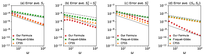
Figure S1: Difference of the one-cycle average calculated from the actual dynamics and that from our formula [Eq. (S35)] (circle), the FGS (square), and the CFSS (triangle) plotted against the driving frequency $\omega$. Each panel shows the result for the observables as described in the panel title. The solid and dashed lines are the guides to the eye showing the lines with slopes $-2$ and $-1$, respectively.

S4.3 One-cycle standard deviations

In the paper, we have discussed the difference of the one-cycle standard deviation $\Delta\Sigma_{A}(\omega)$ for the representative two observables $\hat{A}=\hat{S}_{z}$ and $\{\hat{S}_{x},\hat{S}_{y}\}$. Here we supplement the data, plotting $\Delta\Sigma_{A}(\omega)$ for all the eight observables calculated with our formula [Eqs. (8) and (9)], the FGS (as well as the CFSS for future reference) in Fig. S2.

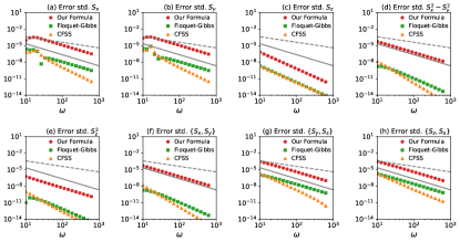
Figure S2: Difference of the one-cycle standard deviation calculated from the actual dynamics and that from our formula [Eq. (S35)] (circle), the FGS (square), and the CFSS (triangle) plotted against the driving frequency $\omega$. Each panel (a-h) shows the result for the observables as described in the panel title. The solid and dashed lines are the guides to the eye showing the lines with slopes $-2$ and $-1$, respectively.

The difference $\Delta\Sigma_{A}(\omega)$ between the actual dynamics and our formula is $O(\omega^{-2})$ for all observables as shown in Fig. S2. This result supports that our micromotion part $\hat{\sigma}_{\text{MM}}(t)$ properly describes the NESS at $O(\omega^{-1})$. Quantitatively, $\Delta\Sigma_{A}(\omega)$ is smaller for the FGS, where all-order contributions in $\omega^{-1}$ are included. We could improve the accuracy of our formula by extending our formula to higher orders.

S5 Breakdown of antiunitary dynamical symmetry

We supplement the argument in the paper that the one-cycle average of $\hat{A}=\{\hat{S}_{x},\hat{S}_{y}\}$ vanishes for the FGS but does not for the actual dynamics and our formulas [Eqs. (8)–(10)]. In the paper, we have shown that the antiunitary operator $\hat{V}$ and the associated dynamical symmetry

$$\hat{V}\hat{H}_{\text{NV}}(T-t)\hat{V}^{\dagger}=\hat{H}_{\text{NV}}(t)$$ (S66)

lead to the vanishing one-cycle average for the FGS. Let us see how such an antiunitary dynamical symmetry does not constrain the actual dynamics or our formula due to dissipation.

First, we discuss the actual dynamics described by the Lindblad equation (S52). To utilize the antiunitary dynamical symmetry, we substitute $t$ by $T-t$ and multiply $\hat{V}$ from left and $\hat{V}^{\dagger}$ from right. Then, we have

$$-\partial_{t}\hat{\rho}^{\hat{V}}(t)=i[\hat{H}_{\text{NV}}(t),\hat{\rho}^{\hat{V}}(t)]+\mathcal{D}^{\prime\prime}[\hat{\rho}^{\hat{V}}(t)],$$ (S67)

where we have used Eq. (S66), $\hat{\rho}^{\hat{V}}(t)\equiv\hat{V}\hat{\rho}(T-t)\hat{V}^{\dagger}$, and $\mathcal{D}^{\prime\prime}$ is defined by $\hat{L}_{ij}\to\hat{L}_{ij}^{\prime\prime}=\hat{V}\hat{L}_{ij}\hat{V}^{\dagger}$ in $\mathcal{D}$. We notice that $\mathcal{D}^{\prime\prime}=\mathcal{D}$ because the time-independent Hamiltonian $\hat{H}_{\text{NV}}^{0}$ is invariant under the antiunitary transform $\hat{V}$ similarly to the argument in Sec. S4.1. Therefore, Eq. (S67) leads to

$$\partial_{t}\hat{\rho}^{\hat{V}}(t)=-i[\hat{H}_{\text{NV}}(t),\hat{\rho}^{\hat{V}}(t)]-\mathcal{D}[\hat{\rho}^{\hat{V}}(t)].$$ (S68)

We note that the sign of the $\mathcal{D}$ term has changed from the original Lindblad equation (S52) and $\hat{\rho}^{\hat{V}}(t)$ cannot be related directly to $\hat{\rho}(t)$. Thus the antiunitary dynamical symmetry (S66) does not constrain the actual dynamics in the presence of dissipation.

Second, we show that our formula is not constrained by the antiunitary dynamical symmetry (S66). More concretely, we have $\hat{V}\hat{\sigma}_{\text{FE}}\hat{V}^{\dagger}\neq\hat{\sigma}_{\text{FE}}$ unlike the case of unitary transformations. To show this, we first notice that the dynamical symmetry (S66) leads to $\hat{V}\hat{H}_{m}\hat{V}^{\dagger}=\hat{H}_{m}$ for the Fourier components and to $\hat{V}\hat{H}_{\mathrm{eff}}\hat{V}^{\dagger}=\hat{H}_{\mathrm{eff}}$ and hence $\hat{V}\varDelta\hat{H}_{\mathrm{eff}}\hat{V}^{\dagger}=\varDelta\hat{H}_{\mathrm{eff}}$. We second notice $\hat{V}=K\hat{U}^{z}_{\pi}$, where $K$ is the complex conjugate operator. Then, we consider the matrix elements of $\hat{V}\hat{\sigma}_{\text{FE}}\hat{V}^{\dagger}$ in the energy eigenbasis:

$$\braket{E_{k}}{\hat{V}\hat{\sigma}_{\text{FE}}\hat{V}^{\dagger}}{E_{l}} =e^{i\theta_{k}}\braket{E_{k}}{K\hat{\sigma}_{\text{FE}}K}{E_{l}}e^{-i\theta_{l}}=e^{i\theta_{k}}\braket{E_{k}}{\hat{\sigma}_{\text{FE}}}{E_{l}}^{*}e^{-i\theta_{l}}$$

$$=\frac{e^{i\theta_{k}}\braket{E_{k}}{\varDelta\hat{H}_{\mathrm{eff}}}{E_{l}}^{*}e^{-i\theta_{l}}}{(E_{k}-E_{l})+i\gamma_{kl}}(p_{\text{can}}^{(k)}-p_{\text{can}}^{(l)})=\frac{\braket{E_{k}}{\hat{U}^{z{\dagger}}_{\pi}\varDelta\hat{H}_{\mathrm{eff}}\hat{U}^{z}_{\pi}}{E_{l}}^{*}}{(E_{k}-E_{l})+i\gamma_{kl}}(p_{\text{can}}^{(k)}-p_{\text{can}}^{(l)})$$

$$=\frac{\braket{E_{k}}{\varDelta\hat{H}_{\mathrm{eff}}}{E_{l}}^{*}}{(E_{k}-E_{l})+i\gamma_{kl}}(p_{\text{can}}^{(k)}-p_{\text{can}}^{(l)})\neq\braket{E_{k}}{\hat{\sigma}_{\text{FE}}}{E_{l}}.$$ (S69)

Although $\braket{E_{k}}{\varDelta\hat{H}_{\mathrm{eff}}}{E_{l}}^{*}=\braket{E_{k}}{\varDelta\hat{H}_{\mathrm{eff}}}{E_{l}}$ in fact, the sign of $\gamma_{kl}$ has changed from $\braket{E_{k}}{\varDelta\hat{H}_{\mathrm{eff}}}{E_{l}}$. Thus, in the presence of dissipation, $\hat{V}\hat{\sigma}_{\text{FE}}\hat{V}^{\dagger}\neq\hat{\sigma}_{\text{FE}}$ and $\text{tr}(\hat{\sigma}_{\text{FE}}\hat{A})\neq 0$ in general even if $\hat{V}\hat{A}\hat{V}^{\dagger}=-\hat{A}$.

S6 Canonical Floquet Steady State (CFSS)

Here we introduce the canonical Floquet steady state (CFSS)

$$\hat{\rho}_{\text{CFSS}}(t)=\frac{1}{Z}\sum_{i}e^{-\beta E_{i}}\ket{u_{i}(t)}\bra{u_{i}(t)}=\frac{1}{Z}\sum_{i}e^{-\beta E_{i}}\ket{\psi_{i}(t)}\bra{\psi_{i}(t)},$$ (S70)

where $Z=\sum_{i}e^{-\beta E_{i}}$, $\ket{u_{i}(t)}$ is the Floquet state, and $\ket{\psi_{i}(t)}=e^{-i\epsilon_{i}t}\ket{u_{i}(t)}$ is the corresponding solution of the time-dependent Schrödinger equation with $\epsilon_{i}$ being the quasienergy. Here, we have assumed that the driving frequency $\omega$ is so large and $\ket{u_{i}(t)}$ is so close to $\ket{E_{i}}$ that there is the one-to-one correspondence between $\ket{E_{i}}$ and $\ket{u_{i}(t)}$ for each index $i$.

The difference between the FGS and CFSS is the weight factor. This is defined by the quasienergy $\epsilon_{i}$ for the FGS whereas by the real energy $E_{i}$ for the CFSS. This difference is quantitatively important because $E_{i}-\epsilon_{i}=O(\omega^{-1})$ and the FGS and CFSS can give different scalings in $\omega$ at high frequency.

The difference of the one-cycle-averaged observables calculated for the actual dynamics and the CFSS is shown in Fig. S1. For the two observables $\hat{S}_{z}$ and $\hat{S}_{z}^{2}$, the CFSS gives the appropriate $\omega^{-2}$ scaling which is not captured by the FGS. For the other two $\hat{S}_{x}^{2}-\hat{S}_{y}^{2}$ and $\{\hat{S}_{x},\hat{S}_{y}\}$, the CFSS deviates from the actual value at $O(\omega^{-1})$ and fails to describe the actual dynamics at $O(\omega^{-1})$. The CFSS thus provide partly improved descriptions for some observables than the FGS. It is noteworthy that the CFSS does not involve any information about the system-bath coupling like the FGS.

The difference of the one-cycle standard deviations $\Delta\Sigma_{A}(\omega)$ calculated for the actual dynamics and the CFSS is shown in Fig. S2. At high-frequency, the CFSS leads to more rapid decreases of $\Delta\Sigma_{A}(\omega)$ than the FGS for most observables. Thus the CFSS gives improved descriptions of the NESS than the FGS.

S7 Equivalence of our formula and CFSS in $\Gamma_{ij}\to 0$

Here we show that, in the weak dissipation limit $\Gamma_{ij}\to 0$, our formula [Eqs. (8)–(10)] coincides with the CFSS rather than the FGS. Since the extension to the degenerate case is straightforward, we consider the case where $\hat{H}_{0}$ is nondegenerate for simplicity.

The weak dissipation limit of our formula is obtained just by replacing $\gamma_{ij}$ with 0 in $\hat{\sigma}_{\text{FE}}$:

$$\hat{\rho}(t)=\hat{\rho}_{\text{can}}+\hat{\sigma}_{\text{MM}}(t)+\hat{\sigma}_{\text{FE}}+O(\omega^{-2}),$$ (S71)

with

$$\braket{E_{k}}{\hat{\sigma}_{\text{FE}}}{E_{l}}=\frac{\braket{E_{k}}{\varDelta\hat{H}_{\mathrm{eff}}}{E_{l}}}{E_{k}-E_{l}}(p_{\text{can}}^{(k)}-p_{\text{can}}^{(l)})\qquad(k\neq l)$$ (S72)

and $\braket{E_{k}}{\hat{\sigma}_{\text{FE}}}{E_{k}}=0$. We will show that $\hat{\rho}_{\text{CFSS}}(t)$ coincides with the above $\hat{\rho}(t)$ by considering its high-frequency expansion.

This is achieved by finding the solution $\ket{\psi_{i}(t)}$ within the high-frequency expansion. According to Ref. Eckardt and Anisimovas (2015), $\ket{\psi_{k}(t)}$ can be represented as

$$\ket{\psi_{k}(t)}=e^{G(t)}\ket{\psi_{k}(0)},$$ (S73)

where

$$G(t)=\frac{1}{\omega}\sum_{m\neq 0}\frac{e^{-im\omega t}}{m}\hat{H}_{m}+O(\omega^{-2}),$$ (S74)

and $\ket{\psi_{k}(0)}$ is the eigenstate of the effective Hamiltonian $\hat{H}_{\mathrm{eff}}=\hat{H}_{0}+\varDelta\hat{H}_{\mathrm{eff}}$ with eigenvalue $\epsilon_{k}=E_{k}+O(\omega^{-1})$. Since $\varDelta\hat{H}_{\mathrm{eff}}=O(\omega^{-1})$ as shown in Sec. S1, $\ket{\psi_{k}(0)}$ can be obtained by the standard perturbation technique as

$$\ket{\psi_{k}(0)}=\ket{E_{k}}+\sum_{l(\neq k)}\ket{E_{l}}\frac{\braket{E_{l}}{\varDelta\hat{H}_{\mathrm{eff}}}{E_{k}}}{E_{k}-E_{l}}+O(\omega^{-2}).$$ (S75)

Substituting this equation into Eq. (S70), we obtain

$$\hat{\rho}_{\text{CFSS}}(t)$$

$$=\sum_{k}p_{\text{can}}^{(k)}e^{G(t)}\left[\ket{E_{k}}\bra{E_{k}}+\sum_{l(\neq k)}\frac{\braket{E_{k}}{\varDelta\hat{H}_{\mathrm{eff}}}{E_{l}}}{E_{k}-E_{l}}\ket{E_{k}}\bra{E_{l}}+\sum_{l(\neq k)}\frac{\braket{E_{l}}{\varDelta\hat{H}_{\mathrm{eff}}}{E_{k}}}{E_{k}-E_{l}}\ket{E_{l}}\bra{E_{k}}\right]e^{-G(t)}+O(\omega^{-2})$$

$$=e^{G(t)}\hat{\rho}_{\text{can}}e^{-G(t)}+\sum_{\begin{subarray}{c}k,l\\ (k\neq l)\end{subarray}}\left[p_{\text{can}}^{(k)}\frac{\braket{E_{k}}{\varDelta\hat{H}_{\mathrm{eff}}}{E_{l}}}{E_{k}-E_{l}}\ket{E_{k}}\bra{E_{l}}+p_{\text{can}}^{(k)}\frac{\braket{E_{l}}{\varDelta\hat{H}_{\mathrm{eff}}}{E_{k}}}{E_{k}-E_{l}}\ket{E_{l}}\bra{E_{k}}\right]+O(\omega^{-2})$$

$$=e^{\mathcal{G}(t)}\hat{\rho}_{\text{can}}+\sum_{\begin{subarray}{c}k,l\\ (k\neq l)\end{subarray}}(p_{\text{can}}^{(k)}-p_{\text{can}}^{(l)})\frac{\braket{E_{k}}{\varDelta\hat{H}_{\mathrm{eff}}}{E_{l}}}{E_{k}-E_{l}}\ket{E_{k}}\bra{E_{l}}+O(\omega^{-2})$$

$$=\hat{\rho}_{\text{can}}+\hat{\sigma}_{\text{MM}}(t)+\hat{\sigma}_{\text{FE}}+O(\omega^{-2}),$$ (S76)

which is equal to our formula (S71) ($\mathcal{G}(t)$ was defined in Sec. S1). We note that the FGS deviates from the CFSS in general by $O(\omega^{-1})$ since $E_{i}-\epsilon_{i}=O(\omega^{-1})$. Thus, in the small dissipation limit, the NESS coincides with the CFSS rather than the FGS.

References

- Holthaus (2015) M. Holthaus, J. Phys. B: At. Mol. Opt. Phys. 49, 13001 (2015).
- Bukov et al. (2015) M. Bukov, L. D’Alessio, and A. Polkovnikov, Advances in Physics 64, 139 (2015).
- Oka and Kitamura (2019) T. Oka and S. Kitamura, Annual Review of Condensed Matter Physics 10, 387 (2019).
- Shirley (1965) J. H. Shirley, Phys. Rev. 138, B979 (1965).
- Eckardt and Anisimovas (2015) A. Eckardt and E. Anisimovas, New Journal of Physics 17, 93039 (2015).
- Mikami et al. (2016) T. Mikami, S. Kitamura, K. Yasuda, N. Tsuji, T. Oka, and H. Aoki, Phys. Rev. B 93, 144307 (2016).
- Lazarides et al. (2014) A. Lazarides, A. Das, and R. Moessner, Phys. Rev. E 90, 12110 (2014).
- Kuwahara et al. (2016) T. Kuwahara, T. Mori, and K. Saito, Annals of Physics 367, 96 (2016), arXiv:1508.05797 .
- Oka and Aoki (2009) T. Oka and H. Aoki, Phys. Rev. B 79, 81406 (2009).
- Wang et al. (2013) Y. H. Wang, H. Steinberg, P. Jarillo-Herrero, and N. Gedik, Science 342, 453 (2013).
- Jotzu et al. (2014) G. Jotzu, M. Messer, R. Desbuquois, M. Lebrat, T. Uehlinger, D. Greif, and T. Esslinger, Nature 515, 237 (2014).
- Rechtsman et al. (2013) M. C. Rechtsman, J. M. Zeuner, Y. Plotnik, Y. Lumer, D. Podolsky, F. Dreisow, S. Nolte, M. Segev, and A. Szameit, Nature 496, 196 (2013).
- Else et al. (2016) D. V. Else, B. Bauer, and C. Nayak, Phys. Rev. Lett. 117, 90402 (2016).
- Choi et al. (2017) S. Choi, J. Choi, R. Landig, G. Kucsko, H. Zhou, J. Isoya, F. Jelezko, S. Onoda, H. Sumiya, V. Khemani, C. von Keyserlingk, N. Y. Yao, E. Demler, and M. D. Lukin, Nature 543, 221 (2017).
- Zhang et al. (2017) J. Zhang, P. W. Hess, A. Kyprianidis, P. Becker, A. Lee, J. Smith, G. Pagano, I.-D. Potirniche, A. C. Potter, A. Vishwanath, N. Y. Yao, and C. Monroe, “Observation of a discrete time crystal,” (2017).
- Sato et al. (2016) M. Sato, S. Takayoshi, and T. Oka, Physical Review Letters 117, 147202 (2016), arXiv:1602.03702 .
- Mentink et al. (2015) J. H. Mentink, K. Balzer, and M. Eckstein, Nature Communications 6, 1 (2015).
- Kohn (2001) W. Kohn, Journal of Statistical Physics 103, 417 (2001).
- Hone et al. (2009) D. W. Hone, R. Ketzmerick, and W. Kohn, Phys. Rev. E 79, 51129 (2009).
- Kohler et al. (1997) S. Kohler, T. Dittrich, and P. Hänggi, Phys. Rev. E 55, 300 (1997).
- Breuer et al. (2000) H.-P. Breuer, W. Huber, and F. Petruccione, Phys. Rev. E 61, 4883 (2000).
- Dehghani et al. (2014) H. Dehghani, T. Oka, and A. Mitra, Phys. Rev. B 90, 195429 (2014).
- Seetharam et al. (2015) K. I. Seetharam, C.-E. Bardyn, N. H. Lindner, M. S. Rudner, and G. Refael, Phys. Rev. X 5, 41050 (2015).
- Schmidt et al. (2019) H.-J. Schmidt, J. Schnack, and M. Holthaus, Physical Review E 100, 42141 (2019).
- Blümel et al. (1991) R. Blümel, A. Buchleitner, R. Graham, L. Sirko, U. Smilansky, and H. Walther, Phys. Rev. A 44, 4521 (1991).
- Vorberg et al. (2013) D. Vorberg, W. Wustmann, R. Ketzmerick, and A. Eckardt, Phys. Rev. Lett. 111, 240405 (2013).
- Kohler et al. (2004) S. Kohler, S. Camalet, M. Strass, J. Lehmann, G.-L. Ingold, and P. Hänggi, Chemical Physics 296, 243 (2004).
- Stefanucci et al. (2008) G. Stefanucci, S. Kurth, A. Rubio, and E. K. U. Gross, Physical Review B 77, 75339 (2008).
- Shirai et al. (2015) T. Shirai, T. Mori, and S. Miyashita, Phys. Rev. E 91, 30101 (2015).
- Shirai et al. (2016) T. Shirai, J. Thingna, T. Mori, S. Denisov, P. Hänggi, and S. Miyashita, New Journal of Physics 18, 53008 (2016).
- Liu (2015) D. E. Liu, Phys. Rev. B 91, 144301 (2015).
- Goldman and Dalibard (2014) N. Goldman and J. Dalibard, Phys. Rev. X 4, 31027 (2014).
- Rahav et al. (2003) S. Rahav, I. Gilary, and S. Fishman, Phys. Rev. A 68, 13820 (2003).
- Dai et al. (2016) C. M. Dai, Z. C. Shi, and X. X. Yi, Phys. Rev. A 93, 32121 (2016).
- Rondin et al. (2014) L. Rondin, J.-P. Tetienne, T. Hingant, J.-F. Roch, P. Maletinsky, and V. Jacques, Reports on Progress in Physics 77, 56503 (2014).
- Ho et al. (1986) T.-S. Ho, K. Wang, and S.-I. Chu, Physical Review A 33, 1798 (1986).
- Prosen and Ilievski (2011) T. Prosen and E. Ilievski, Physical Review Letters 107, 60403 (2011).
- Hartmann et al. (2017) M. Hartmann, D. Poletti, M. Ivanchenko, S. Denisov, and P. Hänggi, New Journal of Physics 19, 83011 (2017).
- Breuer and Petruccione (2002) H. P. Breuer and F. Petruccione, The theory of open quantum systems (Oxford University Press, Great Clarendon Street, 2002).
- Schmidt (2020) H.-J. Schmidt, Journal of Statistical Mechanics: Theory and Experiment 2020, 043204 (2020).
- Note (1) Our results do not contradict the previous studies Shirai et al. (2015, 2016) presenting a set of sufficient conditions for the FGS being valid since our example model does not satisfy these conditions.
- Mananga and Charpentier (2011) E. S. Mananga and T. Charpentier, The Journal of Chemical Physics 135, 44109 (2011).
- Wilcox (1967) R. M. Wilcox, Journal of Mathematical Physics 8, 962 (1967).
Supplemental Material: