A systematic study of $\gamma$-ray flares from the Crab Nebula with Fermi-LAT: I. flare detection

Abstract

Significant flares of GeV $\gamma$-ray emission from the Crab Nebula have been found by AGILE and Fermi-LAT years ago, indicating that extreme particle acceleration and radiation occurs in young pulsar wind nebulae. To enlarge the flare sample and to investigate their statistical properties will be very useful in understanding the nature of the $\gamma$-ray flares. In this paper, we investigate the flaring emission from the Crab Nebula with eleven year observations of the Fermi-LAT. We identify 17 significant flares in the light curve of the low-energy (synchrotron) component of the $\gamma$-ray emission. The flare rate is about 1.5 per year, without any significant change or clustering during the 11 years of the observation. We detect a special flare with an extremely long duration of nearly one month, occurred in October, 2018, with synchrotron photons up to energies of about 1GeV. The synchrotron component could be fitted by a steady power-law background and a variable flare component with an expotentially cutoff power-law spectrum, not only for individual flare but also for the combined data, which may favor a similar emission mechanism for all flares. However, we do not find a universal relation between the cutoff energy and the energy fluxes of the flares, which may reflect the complicated acceleration and/or cooling processes of the involved particles.

1 Introduction

The Crab Nebula, one of the most interesting and well studied objects in the sky, is powered by a young and energetic pulsar, PSR B0531+21, which is a remnant of the supernova recorded by Chinese astronomers in AD 1054. A wind of cold ultra-relativistic particles, accelerated by the rapidly rotating, powerful magnetic fields of the central pulsar, terminates where its momentum flux density is balanced by the confining pressure of the external medium (for young pulsars it may be the ejected stellar material, and for old pulsars it is the interstellar medium). The forming termination shock accelerate high-energy electrons, which lighten the nebula in wide wavebands (Kennel & Coroniti, 1984; Arons & Tavani, 1994). The very broad spectrum of the Crab Nebula can be largely attributed to the synchrotron radiation by relativistic electrons with energies from GeV to PeV (Cocke et al., 1970; Novick et al., 1972; Dean et al., 2008), and the inverse Compton (IC) scattering emission off the cosmic microwave background, the synchrotron nebula, and the thermal dust emission (Gould & Burbidge, 1965; Atoyan & Aharonian, 1996; Meyer et al., 2010).

For a long time, the overall emission from the Crab Nebula was expected to be steady. The Crab Nebula is regarded as a “standard candle” and is usually used to cross-calibrate X-ray and very high energy $\gamma$-ray telescopes (Kirsch et al., 2005; Weisskopf et al., 2010; Meyer et al., 2010). However, the MeV $\gamma$-ray emission seems not that simple. Early observations by COMPTEL and EGRET already showed possible flux variations at a time scale of one year (Much et al., 1995; de Jager et al., 1996). The overall flux in the hard X-ray band also shows shallow changes of a few percents in several years (Wilson-Hodge et al., 2011). Surprisingly strong flares have been found for energies above 100 MeV, by AGILE (Tavani et al., 2011) and Fermi-LAT (Abdo et al., 2011). Later several more flares have been reported (Striani et al., 2011; Buehler et al., 2012; Mayer et al., 2013; Striani et al., 2013), with a super-giant one occurred in April, 2011. Dedicated efforts have been paid to search for possible counterparts of the $\gamma$-ray flares in other wavelengths, but no firm counterpart has been found yet (Lobanov et al., 2011; Bartoli et al., 2012; Weisskopf et al., 2013; Bühler & Blandford, 2014; H. E. S. S. Collaboration et al., 2014; Aliu et al., 2014; Aleksić et al., 2015; Rudy et al., 2015).

Various models have been proposed to explain the $\gamma$-ray flares, with particular focus on the puzzle that how could electrons generate synchrotron radiation above a maximum energy of $\sim 160$ MeV for the classical shock acceleration (Guilbert et al., 1983; Uzdensky et al., 2011), and what is the location of the emission sites where rapid variability on a timescale of hours could be produced. A widely adopted way to produce synchrotron emission up to GeV energies is the Doppler boosting of the emission site (Cheng & Wei, 1996; Komissarov & Lyutikov, 2011; Yuan et al., 2011; Kohri et al., 2012). Alternatively, the magnetic reconnection induces a linear electric accelerator which can also overcome such a difficulty (Uzdensky et al., 2011; Cerutti et al., 2012a, b, 2013, 2014; Yuan et al., 2016; Zrake & Arons, 2017; Lyutikov et al., 2017a, b). As for the flare site, in Komissarov & Lyutikov (2011) it was proposed that the observed synchrotron $\gamma$-rays would be dominated by the contribution of the inner knot, whose size is about a few light days and is consistent with the flare duration. Also the emissions from the inner knot would be blue-shifted and can exceed the $160$ MeV limit. Rapid changes of the shock geometry due to the violent dynamics of the inner nebula may produce the observed variability (Komissarov & Lyutikov, 2011; Lyutikov et al., 2012), with a possible caveat that no correlated variability in various energy bands was observed (Rudy et al., 2015). Bednarek & Idec (2011) suggested that electrons are accelerated in a region behind the shock, and the variability is attributed to changes in the maximum energy of accelerated electrons, electron spectral index, or the magnetic field. This scenario predicts multi-TeV $\gamma$-ray variabilities as a result of the IC emission which is lacking. Kirk & Giacinti (2017) proposed that the frequency, variability and power of the flares emerge as natural consequences of a sharp reduction of the supply of electron-positron pairs to the wind of the Crab pulsar, furthermore the polarization properties of the flares and possible similar emission from other pulsar wind nebulae are predicted.

Previous works for the analysis of the $\gamma$-ray flares from the Crab Nebula were generally based on case studies (Tavani et al., 2011; Abdo et al., 2011; Buehler et al., 2012; Striani et al., 2011; Mayer et al., 2013). Given the long-term operation of Fermi-LAT for more than 10 years, it is expected that more $\gamma$-ray flares would be detected, and it is highly desired to have a population study of the flares. This is the motivation of the current study. The statistical characterization of the flare properties is expected to be very useful in revealing the physical nature of the flares (Yuan & Wang, 2016; Yuan et al., 2018), which will be studied in details in an accompanying work. The structure of this paper is as follows. In Section 2 we calculate the folded pulsar phase of each photon based on radio observations in order to remove the strong pulsar emission. We then extract $\gamma$-ray flares from 11 years of observations of the Fermi-LAT in Section 3, and carry out a case study for the ultra-long duration flare occurred in October, 2018, in Section 4. In Section 5 we investigate briefly the properties of all detected flares. We discuss the possible implications of our results in Section 6, and then conclude our study in Section 7.

2 Phase folding of the central pulsar

The Crab pulsar, PSR B0531+21, one of the most energetic known pulsars (with a spin down power of $\dot{E}=4.6\times 10^{38}$ erg s^-1), lies at the center of the Crab Nebula. To remove the strong $\gamma$-ray emission from this pulsar, we need to calculate the phase of each photon and to select photons in the off-pulse window for the following analysis about the nebula.

The rotation rate of the Crab pulsar, like many young pulsars, is affected by significant timing noise and glitches. Since we will cover a relatively long time interval in this paper, the rotational behavior evolution with time needs to be known with a very high precision. The Jodrell Bank Observatory has continuously made the monthly ephemeris of the Crab pulsar for decades (Lyne et al., 1993). These monthly ephemeris data give the primary spin frequency (F0), the first derivative (F1), the rate at which the pulsar slows down, and also the second derivative (F2) which gives the timing noise, of the Crab pulsar for time windows lasting about one month each. With these ephemeris data we can use the TEMPO2, a pulsar analysis package developed by radio astronomers, to assign phases to $\gamma$-ray photons collected by the Fermi-LAT with the help of a plugin. We also assume that the rotation of the Crab pulsar will not change significantly in a short time. Therefore for photons with arrival times outside a given time window as defined in the monthly JODRELL BANK CRAB PULSAR MONTHLY EPHEMERIS, it is still fine to calculate the phase using the nearby ephemeris. A match of the phases calculated using the previous ephemeris and the successive one has been applied.

We use the Fermi-LAT data collected from August 4, 2008 to October 24, 2019. The events that pass the P8R3 SOURCE event class selections with energies from 80 MeV to 300 GeV and angles within 25 degrees from the Crab pulsar are selected. Here we select photons with energies down to 80 MeV and angles within 25 degrees from the target source to get more photons to calculate the pulsar phases more accurately. The folded light curve in pulsar phase for three periods are shown in Fig. 1. The separation into three time periods are based on the times when two significant glitches happened on November 10, 2011 and November 8, 2017.

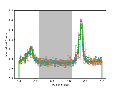
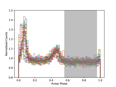
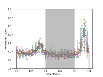
Figure 1: The phase-folded light curves in three time intervals, from MJD 54682 to MJD 55876 (top), from MJD 55876 to MJD 58063 (middle), and from MJD 58065 to MJD 58788 (bottom), respectively. In each panel, the thin histograms show light curves for photons selected in each time window defined in the JODRELL BANK CRAB PULSAR MONTHLY EPHEMERIS, and thick one shows the combined light curve for all photons in this time period. The grey region in each panel shows the off-pulse window used for the following Crab Nebula analysis.

3 Crab flares from the Fermi-LAT data

We re-select $\gamma$-ray photons that pass the P8R3 SOURCE event class selection, with energies from 100 MeV to 300 GeV and angular deviations within 15 degrees from the Crab pulsar for the flare analysis. For the three time intervals defined in Fig. 1, the off-pulse phase ranges are defined as 0.24 to 0.64, 0.56 to 0.96, and 0.40 to 0.80, as shown in gray bands in Fig. 1. Photons collected at zenith angles larger than 90^∘ are removed to suppress the contamination from $\gamma$-rays generated by cosmic-ray interactions in the upper layers of the atmosphere. Moreover, we filter the data using the following specifications (DATA$\_$QUAL$>$0) $\&\&$ (LAT$\_$CONFIG==1) $\&\&$ (angsep (83.63, 22.01, RA$\_$SUN, DEC$\_$SUN)$>$15) to select the good time intervals in which the satellite is working in the standard data taking mode and the data quality is good, and to exclude times when the Crab nebula is within 15 degrees of the Sun to suppress the contamination from the Sun’s activities. We employ the unbinned likelihood analysis method to analyze the data with the Fermitools version 1.2.1. The instrument response function (IRF) adopted is P8R3_SOURCE_V2. For the diffuse background emissions we take the Galactic diffuse model gll_iem_v07.fits and the isotropic background spectrum iso_P8R3_SOURCE_V2_v1.txt as recommended by the Fermi-LAT collaboration. The source model XML file is generated using the user contributed tool make4FGLxml.py based on the 4FGL source catalog (Abdollahi et al., 2020). Following Abdo et al. (2010), we assume the emission from the Crab Nebula consists of two spectral components, high-energy component for IC emission and low-energy component for synchrotron emission, each with a power-law (PL) spectrum, $dN/dE\propto E^{-\Gamma_{i}}$, taking $i=h,l$ for high and low energy component, respectively.

We perform an unbinned maximum likelihood fit with the module pyLikelihood in the Fermitools for each time interval, and use the module SummedLikelihood to perform a joint likelihood analysis of all the three time intervals. For the joint analysis, the integrated flux above 100 MeV of the low-energy component is found to be $\Phi_{100}=(8.84\pm 0.08)\times 10^{-7}$ cm^-2 s^-1, and the photon index is $\Gamma_{l}=3.63\pm 0.03$, and the high-energy component has an integral flux of $\Phi_{100}=(1.73\pm 0.06)\times 10^{-7}$ cm^-2 s^-1 and $\Gamma_{h}=1.73\pm 0.01$. Compared with parameters derived in Abdo et al. (2010, 2011), we got a good agreement with spectral indices for those two components, but the integrated fluxes are higher. For each time intervals, we also derive the fitting results of these two components. As shown in Fig. 2 the integrated fluxes for each time interval are almost consistent with that from the joint likelihood analysis, except for the flux of the low-energy component in the third time interval. A higher value of the flux of the low-energy component in the third time interval is possibly due to the long-duration flare occurred in October, 2018 (see Section 4).

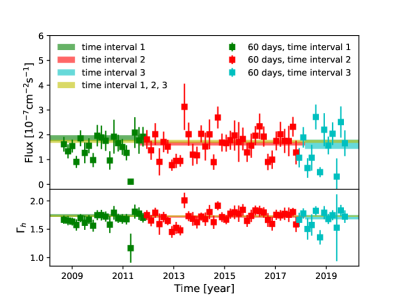
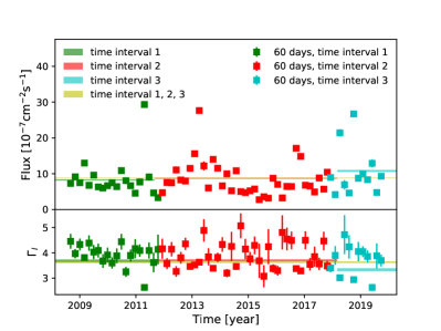
Figure 2: Fluxes and spectral indices of the high-energy (IC emission, top panel) and low-energy (synchrotron emission, bottom panel) components in 60-day binning. The shaded bands in each panel show the fluxes and spectral indices from the likelihood fits done for the three time intervals individually, and that from the joint fit.

Fig. 2 shows the light curves and spectral indices of the high-energy (top) and low-energy (bottom) components for a bin width of 60 days. For each time bin, the free parameters in the likelihood fit include the normalizations and spectral indices of the (both) nebula components, and the normalizations of the Galactic and isotropic diffuse backgrounds. All other parameters are fixed to their best-fit values from the joint likelihood analysis. It is clear that the flux of high-energy component is stable with fluctuations within $3\sigma$ from the average flux. An only exception is the bin around April, 2011. However, the fluxes of the low-energy component show significant variations. The highest flux bins show more than 4 times higher fluxes than the average one, and have more than $30\sigma$ deviations.

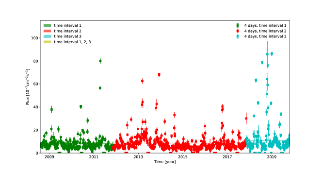
Figure 3: Same as the light curves in the bottom panel of Fig. 2 but for 4-day binning.

To see the varibilities more clearly, we re-bin the data into a bin width of 4 days, and re-fit the data with only the normalizations and spectral indices of the low-energy component being free parameters. The high-energy component normalizations and spectral indices and the Galactic and isotropic diffuse background normalizations are fixed to their best-fit values derived in the joint analysis. The light curve of the low-energy component in 4-day time bin is shown in Fig. 3.

To define a flare, there are some sophisticated statistical methods in the literature, including the Bayesian block method (Scargle et al., 2013), the sequential analysis and change point analysis (Tartakovsky, 2019), autoregressive modeling (Box et al., 2015; Feigelson et al., 2018; Hyndman, 2018; Chatfield & Xing, 2019) and template fitting (Davenport, 2016). But here we use a straight forward method to identify significant flares by selecting time bins with $5\sigma$ higher fluxes compared with the average one, $(8.45\pm 0.08)\times 10^{-7}$ cm^-2 s^-1. If there are several times are adjacent, they are defined as a single flare. We also try to use the Bayesian block method to detect flares (Scargle et al., 2013). However, since the bin-by-bin variation is too large, the Bayesian block method does not work efficiently for this light curve with 11 years data, and we only use it to detect flux variation of these identified flares in the following sections. For the 11 years of the Fermi-LAT data, we find 17 such flares distributed in 35 time bins. All the flares reported before are detected using the above method. They are flare #1 (Abdo et al., 2011), flare #2 (Tavani et al., 2011; Abdo et al., 2011), flare #3 (Buehler et al., 2012; Striani et al., 2011), and flare #6 (Mayer et al., 2013). Light curves and outburst times of the 17 flares are shown in Fig.  4.

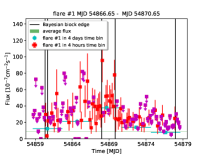
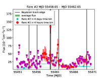
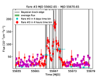
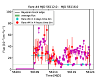
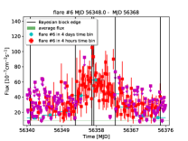
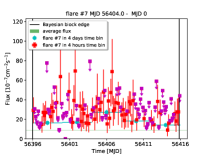
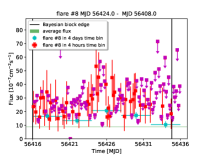
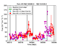
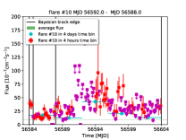
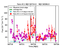
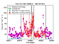
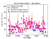
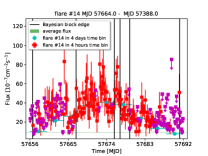
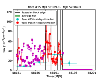
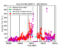
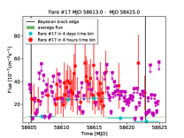
Figure 4: Light curves of the low-energy component in 4-day binning, red for measured points and magenta for upper limits, and 4-hour binning, cyan for measured points and blue for upper limits, for the 17 detected flares in 11 year observations of the Fermi-LAT. Edges defined by Bayesian block are shown in black vertical lines. Average flux of the low-energy component in the whole observational time is in green band.

4 The October 2018 flare

As can be seen in Fig.  3, there is a very-long-duration flare occurred in October, 2018 (flare #16), whose duration is about one month. This is by far the longest duration flare reported for the Crab Nebula. The light curve, in 4-day binning, of the $\gamma$-ray fluxes of this flare is shown in Fig. 5, where we add two more bins (8 days of data) before (after) the first (last) bin of the flare to easily see the rise of flare from the steady state. To get more details about this flare, we make the light curve with a bin width of 4 hours and use the Bayesian block method (Scargle et al., 2013), with a false positive rate of 0.07 , to determine the time windows, which contain information about variations of the flux. It seems that there are two sub-flares, peaking around MJD 58408 and MJD 58419. The rise of the first sub-flare is very slow, taking more than ten days to reach its peak. However, since there is not enough data between MJD 58411 and MJD 58416, when the exposure at the position of the Crab Nebula is very low or even zero as in the bottom panel of Fig. 5, we can not get enough information about the decay of the first sub-flare and the rise of the second sub-flare. The decay time is approximately 1.5 days for the second sub-flare. A second rise or “shoulder”, around MJD 58410 and MJD 58420 with low significance, could be seen by eyes during the decaying phase of both sub-flares, similar to the flare happened in the April of 2011 (Buehler et al., 2012), but the second rise of the second sub-flare has almost the same or even higher flux as its first rise.

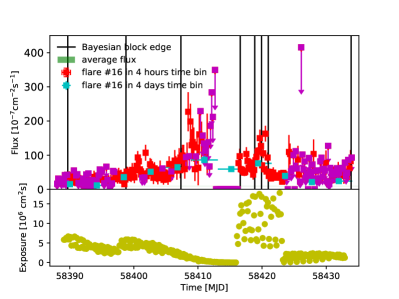
Figure 5: Top: Light curves of the low-energy component in 4-day binning red for measured points and magenta for upper limits, and 4-hour binning, cyan for measured points, for the October 2018 flare. Edges defined by Bayesian block are shown in black vertical lines. Average flux of the low-energy component in the whole observational time is in green band. Bottom: The Exposure at the position of the Crab for every 4-hour observation around 100 MeV.

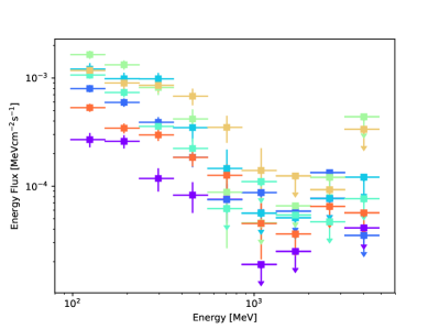
Figure 6: The SEDs of the 7 time bins, defined by the Bayesian block method, for the low-energy component of the October 2018 flare.

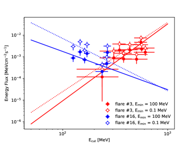
Figure 7: The energy flux versus the cutoff energy of the flare component for flare #3 and flare #16. Two minimum energies are used to get those energy fluxes. And a PL function is used to fit the relationship.

For the 7 time bins defined by the Bayesian block method, we derive their spectral energy distributions (SED) of the low-energy component, through dividing the data into 9 logarithmically evenly distributed energy bins from 100 MeV to 5 GeV to cover the energy range of the low-energy component, for each time bin. Only the normalizations of the low-energy component are set free during the SED fits, while other parameters are fixed as best fit values evaluated in the previous section for the joint likelihood analysis of all time intervals. If the significance is lower than $2\sigma$ in particular energy bins, the 95% upper limits are derived. The results are given in Fig. 6. One SED, corresponding to the time window from MJD 58419.5 to MJD 58420.5, has data point reaching 1 GeV.

Following Buehler et al. (2012) we assume that the total emission of the low-energy component could be further composed of two components, a steady background and a flare component, which is assumed to only contribute to the low energy part considering no firm detection at very-high energy yet (Bartoli et al., 2012; H. E. S. S. Collaboration et al., 2014; Aliu et al., 2014; Aleksić et al., 2015). A PL model, $dN/dE\propto E^{-\Gamma_{b}}$, is adopted to describe the background emission, and a power-law with an exponential cutoff (PLEC), $dN/dE\propto E^{-\Gamma_{f}}exp(-E/E_{cut})$, is used to describe the flare emission. The steady background component and the index $\Gamma_{f}$ of the flare component are assumed to be the same in all time windows, but the normalization and the cutoff energy $E_{\rm cut}$ are free parameters for each time window. Using the module Composite2 in the Fermitools, we fit all the 7 time bins simultaneously. The integrated flux of the steady component is $\Phi_{100}=(9.53\pm 2.06)\times 10^{-7}$ cm^-2 s^-1, and the spectral index is $\Gamma_{b}=4.06\pm 0.07$. The spectral index of the flare component, $\Gamma_{f}$, is derived to be $1.33\pm 0.25$. To check the validity of our method, we also use the same method to re-analyze the April 2011 flare (flare #3), and we get $\Phi_{100}=(9.90\pm 3.27)\times 10^{-7}$ cm^-2 s^-1, $\Gamma_{b}=3.53\pm 0.28$ and $\Gamma_{f}$= $1.37\pm 0.12$. All these results, especially the spectral index of the flare component of these two flares, are consistent with those derived for the April 2011 flare in Buehler et al. (2012), where they get $\Phi_{100}=(5.4\pm 5.2)\times 10^{-7}$ cm^-2 s^-1, $\Gamma_{b}=3.9\pm 1.3$ and $\Gamma_{f}$= $1.27\pm 0.12$.

We plot in Fig. 7 the fitting results of the cutoff energies, $E_{\rm cut}$, and the energy flux, $F$, of the flare component for both flares, flare #3 and flare #16. Following Buehler et al. (2012), we use a PL function $F=\alpha E_{\rm cut}^{\beta}$ to fit the relationship between both quantities. We first set $E_{\rm min}$ to 100 MeV to get the energy flux. For flare #3, we have $\beta=3.55\pm 1.37$, which is consistent with previous result (Buehler et al., 2012). But for flare #16, we get $\beta=-1.76\pm 0.88$, which shows a different relationship between $E_{\rm cut}$ and $F$. For flare #16, some of the cutoff energy are close to 100 MeV, and choosing 100 MeV as $E_{\rm min}$ to get the energy flux will lead to more underestimation of the energy associated with these low cutoff energy time window. Here we also test to switch $E_{\rm min}$ to 0.1 MeV, and as in Fig.  7 this would make $\beta$ smaller for both flares and lead to larger deviation between $\beta$ derived for these two flares, with $\beta=3.20\pm 1.31$ and $\beta=-2.41\pm 0.89$, respectively.

Thus for this October 2018 flare (flare #16), it could be decomposed into a steady background component, which has consistent parameters as the steady background component of flare #3, and a flare component, which also has a consistent spectral index as the flare component of flare #3. This indicates that these two flares may share similar mechanism behind them. However there may be a discrepancy between indexes $\beta$, which shows the relationship between the energy flux and the cutoff energy of the flare component, derived from these two flares, and this may lead to more complicated modelling for the emission mechanism.

5 Properties of the flares

As shown in Section 4, flares occurred in April, 2011 and October, 2018 may share the same steady background and the same spectral index for the flare component, thus we may expect that all 17 flares will share these parameters, only varying the normalization and cutoff energy to account for their difference. Then the same as for flare #16, we make light curves with a bin width of 4 hours for each flare identified in Section 3, and use the Bayesian block method to determine time windows, as shown in Fig.  4. Using the module Composite2 in the Fermitools, we fit the normalization and the cutoff energy of flare component for each time window, spectral index for the flare component and parameters for the steady background component simultaneously. This composite likelihood analysis gives an integrated flux of the steady background component $\Phi_{100}=(8.22\pm 1.14)\times 10^{-7}$ cm^-2 s^-1 above 100 MeV, a spectral index $\Gamma_{b}=3.80\pm 0.15$, and a spectral index of the flare component $\Gamma_{f}=1.39\pm 0.08$. As expected, these parameters, derived by combining all identified flares, are consistent with those derived from analysis for individual flare, and this may indicate all flares would share the same emission mechanism.

We plot, in Fig. 8, the fitting results of the cutoff energies and the energy flux, with $E_{\rm min}=0.1$ MeV, of the flare component for all time windows associated with identified flares, excluding those with TS $<$ 25 and those with $E_{\rm cut}$ $<$ 100 MeV, which may be not so reliable considering our data are all above 100 MeV. Using a PL function $F=\alpha E_{\rm cut}^{\beta}$ to fit the results gives $\beta=1.57\pm 0.33$, with a reduced $\chi^{2}$ of about 3.03 for a number of degrees of freedom (dof) 37. Motivated by possibly different $\beta$ for flare #3 and flare #16, we use a broken power-law, $F=\alpha(E_{\rm cut}/E_{\rm break})^{\beta_{1}}$ for $E_{\rm cut}<E_{\rm break}$ and $F=\alpha(E_{\rm cut}/E_{\rm break})^{\beta_{2}}$ for $E_{\rm cut}>E_{\rm break}$, to fit the relationship between the cutoff energy and energy flux. This would give a better fit, compared with the PL function, with a reduced $\chi^{2}$ of about 1.88 for a number of dof 35. And this would give a break energy, $215.50\pm 19.00$ MeV, the index $\beta_{1}=-4.16\pm 1.32$, and the index $\beta_{2}=2.56\pm 0.61$. And there is a marginal consistency, between $\beta_{1}$ and $\beta$ derived for flare #16, and between $\beta_{2}$ and $\beta$ derived for flare #3. These may suggest there are two groups of flares, as hinted in Section 4, and some mechanisms, other than Doppler boosting, may be needed.

To further investigate the possible effect by the width of the time bin, we repeat all the analyses with time bin widths fixed to 4 days. And we get the integrated flux of the steady background component $\Phi_{100}=(6.55\pm 3.34)\times 10^{-7}$ cm^-2 s^-1 above 100 MeV, a spectral index $\Gamma_{b}=3.55\pm 0.25$, and a spectral index of the flare component $\Gamma_{f}=1.52\pm 0.22$, which are all consistent with those derived previously. A PL function and a broken power-law are used to fit the relationship between the cutoff energy and the energy flux of each time bin, as shown in Fig. 9, and still a broken power-law, with one index negative and another index positive, is weakly preferred.

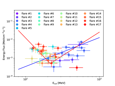
Figure 8: The energy flux versus the cutoff energy of the flare component for all identified flares together. Different colors are used to indicate points associated with different flares. 0.1 MeV is used as the minimum energy to get those energy fluxes. A PL function and a broken power-law are fitted, and are shown in blue and red line.

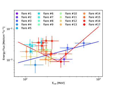
Figure 9: Same as Fig. 8, but the time bin is fixed to 4-days for all flares.

Table 1: Parameters about the flux above 100 MeV and the index of the steady background, the index of the flare component and parameters for the relationship between the cutoff energy and the energy flux above 0.1 MeV of the flare component. Parameters from individual flare, flare #16 and flare #3, and from all flares together are shown. For comparison, we also list parameters for flare #3 from (Buehler et al., 2012), where they consider energy flux above 100 MeV to get $\beta$, and we list parameters derived for all flares, with fixed 4-day binning .

	flare #16 (Bayesian block)	flare #3 (Bayesian block)	flare #3 (Buehler et al., 2012)	all flares (Bayesian block)	all flares (4-day binning)
$\Phi_{100}$ $(10^{-7}$ cm-2 s${}^{-1})$	9.53 $\pm$ 2.06	9.90 $\pm$ 3.27	5.4 $\pm$ 5.2	8.22 $\pm$ 1.14	6.55 $\pm$ 3.34
$\Gamma_{b}$	4.06 $\pm$ 0.07	3.53 $\pm$ 0.28	3.9 $\pm$ 1.3	3.80 $\pm$ 0.15	3.55 $\pm$ 0.25
$\Gamma_{f}$	1.33 $\pm$ 0.25	1.37 $\pm$ 0.12	1.27 $\pm$ 0.12	1.39 $\pm$ 0.08	1.52 $\pm$ 0.22
$\beta$	-2.41 $\pm$ 0.89	3.20 $\pm$ 1.31	3.42 $\pm$ 0.86	1.57 $\pm$ 0.33	0.62 $\pm$ 0.25
$\beta_{1}$, $\beta_{2}$				-4.16 $\pm$ 1.32, 2.56 $\pm$ 0.61	-1.14 $\pm$ 0.48, 2.01 $\pm$ 1.27

6 Discussion

In the 11 years of the observational data, we identify 17 significant flares, which corresponds to a flare rate of $\sim 1.5$ yr^-1. It would be interesting to explore the potential long-term change of the flare rate, and to search for possible clustering of the flares (Yuan & Wang, 2016). We calculate the cumulative number of flares as a function of time. The nearly linear increase of the number with time, as shown in the top panel of Fig. 10, suggests that the flare rate is approximately constant during the observations. The Kolmogorov-Smirnov (KS) test of the data versus the constant expectation gives a probability of $P_{\rm KS}=0.633$. We also calculate the cumulative distribution of the waiting time between successive flares, as given in the bottom panel of Fig. 10. Compared with the null hypothesis in which flares occur randomly with an exponential distribution of the waiting time, $dN/d(\Delta t)\propto\exp(-\Delta t/\overline{\Delta t})$ with $\overline{\Delta t}$ being the mean waiting time from the 17 detected flares, the occur rate of flares is consistent with a stationary Poisson process with a constant rate. The current data do not show any significant clustering of the flare rate.

Our work shows that not only individual flare, but all flares together, could be decomposed into a steady background component and a varying flare component. And as summarized in Table 1, the flux and the index $\Gamma_{b}$ of the background component, and the index $\Gamma_{f}$ of the flare component are consistent for all cases. This may be a strong indication that all flares would share the same emission mechanism. But for the relationship between the cutoff energy and the energy flux, there is a break between 200 to 300 MeV. As hinted by colors for different flares in Fig. 8, there may be two groups of flares, one, such as flare #3, with large cutoff energies and a positive index for a PL function, and the other, such as flare #16, with low cutoff energies and a negative index for a PL function . The positive index, which is about 3, is consistent with that expected for the Doppler boosting scenario of the flare emission. But the physical interpretation for the negative index would need investigation in future works. We also note that the goodness for the fitting of the relationship is not good, even for the broken power-law case, with a reduced $\chi^{2}$ of about 1.88 for a number of dof 35. This may be due to the intrinsic dispersion of different flares.

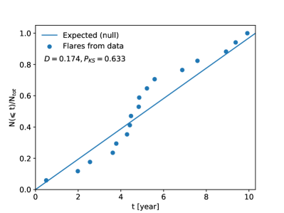
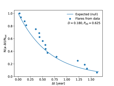
Figure 10: Normalized cumulative number of flares as a function of time (top) and the normalized cumulative distribution of the waiting time (bottom).

7 Conclusion

Energetic flares have been revealed in the $\gamma$-ray band from the Crab Nebula by AGILE and Fermi-LAT (Tavani et al., 2011; Abdo et al., 2011; Buehler et al., 2012; Striani et al., 2011; Mayer et al., 2013). Using the eleven years of the Fermi-LAT data, we carry out a systematic search for flares from the Crab Nebula in this work. We confirm that the flux of high-energy component was stable with deviations from the average flux $<3\sigma$. The low-energy component is found to be highly variable. We identify 17 significant flares from 2008 to 2019, which correspond to a flare rate of $\sim 1.5$ yr^-1. The data is consistent with a random occur rate of flares, without significant clustering of the flares.

We have done a case study for the longest duration flare occurred in October, 2018. We have a detection of synchrotron photons up to energies of about 1 GeV. And we also find it could be decomposed in a similar way, with a steady soft PL component and a variable PLEC flaring component, as the strong flare occurred in April, 2011, with consistent parameters. But the relationship between the cutoff energy and the energy flux is different from that for the flare occurred in April, 2011, with a negative index.

We make a similar decomposition for all identified flares as we did for individual flare, and we get a consistent description for the steady background component and the index of the flare component. In this case, the steady component has a PL index of $3.80\pm 0.15$, which may correspond to the synchrotron tail of the accelerated electrons of the overall nebula. The PL index of the flare component is much harder, $\Gamma=1.39\pm 0.08$, with an exponential cutoff which varies flare by flare (or even bin by bin for the same flare). This consistent picture may suggest that all flares would share similar emission mechanism. And the cutoff energies often, about 82% of points in the Fig. 8, exceed the $\sim 160$ MeV synchrotron limit of diffusive shock acceleration models, indicating the existence of Doppler boosting or special acceleration mechanisms (Komissarov & Lyutikov, 2011; Yuan et al., 2011; Kohri et al., 2012; Uzdensky et al., 2011). But we also find that, compared with a PL, a broken power-law could better fit the relationship between the cutoff energy and the energy flux of these flares. And for the best fitted broken power-law, one index is consistent with that derived for the flare occurred in October, 2018 and another index is consistent with that derived for the flare occurred in April, 2011. While the positive index around 3 is consistent with the Doppler boosting scenario of the flare emission, but the negative index needs further investigation.

Finally we emphasize that the statistical properties of the detected flares should be useful in understanding the physical mechanism of the flare production. A dedicated statistical study with template fitting method for flare detection, with a focus on the flare energy distribution, duration distribution, and the energy-duration correlation, will be published elsewhere.

Appendix A Photon Selection with different pulsar phases

To check the effect of the photon selection with different pulsar rotational phases, we follow the procedure in Section 3 but choose photons with narrower phases, from 0.29 to 0.59, from 0.61 to 0.91, and from 0.45 to 0.75 for the three time intervals, respectively. The light curve of the low-energy component is shown in Fig. 11. For almost all time bins, the fluxes derived from data with shorter phase cuts are consistent with that derived from data with original phase cuts. The results of our analysis should be affected little by the phase cuts.

Figure 11: Same as Fig. 3 but overploted with the results for more strict phase cuts.

References

- Abdo et al. (2010) Abdo, A. A., Ackermann, M., Ajello, M., et al. 2010, ApJ, 708, 1254
- Abdo et al. (2011) —. 2011, Science, 331, 739
- Abdollahi et al. (2020) Abdollahi, S., Acero, F., Ackermann, M., et al. 2020, ApJS, 247, 33
- Aleksić et al. (2015) Aleksić, J., Ansoldi, S., Antonelli, L. A., et al. 2015, Journal of High Energy Astrophysics, 5, 30
- Aliu et al. (2014) Aliu, E., Archambault, S., Aune, T., et al. 2014, ApJ, 781, L11
- Arons & Tavani (1994) Arons, J., & Tavani, M. 1994, ApJS, 90, 797
- Atoyan & Aharonian (1996) Atoyan, A. M., & Aharonian, F. A. 1996, MNRAS, 278, 525
- Bartoli et al. (2012) Bartoli, B., Bernardini, P., Bi, X. J., et al. 2012, The Astronomer’s Telegram, 4258, 1
- Bednarek & Idec (2011) Bednarek, W., & Idec, W. 2011, MNRAS, 414, 2229
- Box et al. (2015) Box, G. E. P., Jenkins, G. M., Reinsel, G. C., & Ljung, G. M. 2015, Time Series Analysis: Forecasting and Control (Wiley), 712p
- Buehler et al. (2012) Buehler, R., Scargle, J. D., Blandford, R. D., et al. 2012, ApJ, 749, 26
- Bühler & Blandford (2014) Bühler, R., & Blandford, R. 2014, Reports on Progress in Physics, 77, 066901
- Cerutti et al. (2012a) Cerutti, B., Uzdensky, D. A., & Begelman, M. C. 2012a, ApJ, 746, 148
- Cerutti et al. (2012b) Cerutti, B., Werner, G. R., Uzdensky, D. A., & Begelman, M. C. 2012b, ApJ, 754, L33
- Cerutti et al. (2013) —. 2013, ApJ, 770, 147
- Cerutti et al. (2014) —. 2014, Physics of Plasmas, 21, 056501
- Chatfield & Xing (2019) Chatfield, C., & Xing, H. 2019, The Analysis of Time Series: An Introduction with R (Chapman and Hall/CRC), 414p
- Cheng & Wei (1996) Cheng, K. S., & Wei, D. M. 1996, MNRAS, 283, L133
- Cocke et al. (1970) Cocke, W. J., Disney, M. J., Muncaster, G. W., & Gehrels, T. 1970, Nature, 227, 1327 EP
- Davenport (2016) Davenport, J. R. A. 2016, ApJ, 829, 23
- de Jager et al. (1996) de Jager, O. C., Harding, A. K., Michelson, P. F., et al. 1996, ApJ, 457, 253
- Dean et al. (2008) Dean, A. J., Clark, D. J., Stephen, J. B., et al. 2008, Science, 321, 1183
- Feigelson et al. (2018) Feigelson, E. D., Babu, G. J., & Caceres, G. A. 2018, Frontiers in Physics, 6, 80
- Gould & Burbidge (1965) Gould, R. J., & Burbidge, G. R. 1965, Annales d’Astrophysique, 28, 171
- Guilbert et al. (1983) Guilbert, P. W., Fabian, A. C., & Rees, M. J. 1983, MNRAS, 205, 593
- H. E. S. S. Collaboration et al. (2014) H. E. S. S. Collaboration, Abramowski, A., Aharonian, F., et al. 2014, A&A, 562, L4
- Hyndman (2018) Hyndman, R. J. 2018, Forecasting: principles and practice (OTexts), 382p
- Kennel & Coroniti (1984) Kennel, C. F., & Coroniti, F. V. 1984, ApJ, 283, 694
- Kirk & Giacinti (2017) Kirk, J. G., & Giacinti, G. 2017, Phys. Rev. Lett., 119, 211101
- Kirsch et al. (2005) Kirsch, M. G., Briel, U. G., Burrows, D., et al. 2005, in Society of Photo-Optical Instrumentation Engineers (SPIE) Conference Series, Vol. 5898, UV, X-Ray, and Gamma-Ray Space Instrumentation for Astronomy XIV, ed. O. H. W. Siegmund, 22–33
- Kohri et al. (2012) Kohri, K., Ohira, Y., & Ioka, K. 2012, MNRAS, 424, 2249
- Komissarov & Lyutikov (2011) Komissarov, S. S., & Lyutikov, M. 2011, MNRAS, 414, 2017
- Lobanov et al. (2011) Lobanov, A. P., Horns, D., & Muxlow, T. W. B. 2011, A&A, 533, A10
- Lyne et al. (1993) Lyne, A. G., Pritchard, R. S., & Graham-Smith, F. 1993, MNRAS, 265, 1003
- Lyutikov et al. (2012) Lyutikov, M., Balsara, D., & Matthews, C. 2012, MNRAS, 422, 3118
- Lyutikov et al. (2017a) Lyutikov, M., Sironi, L., Komissarov, S. S., & Porth, O. 2017a, Journal of Plasma Physics, 83, 635830601
- Lyutikov et al. (2017b) —. 2017b, Journal of Plasma Physics, 83, 635830602
- Mayer et al. (2013) Mayer, M., Buehler, R., Hays, E., et al. 2013, ApJ, 775, L37
- Meyer et al. (2010) Meyer, M., Horns, D., & Zechlin, H.-S. 2010, A&A, 523, A2
- Much et al. (1995) Much, R., Bennett, K., Buccheri, R., et al. 1995, A&A, 299, 435
- Novick et al. (1972) Novick, R., Weisskopf, M. C., Berthelsdorf, R., Linke, R., & Wolff, R. S. 1972, ApJ, 174, L1
- Rudy et al. (2015) Rudy, A., Horns, D., DeLuca, A., et al. 2015, ApJ, 811, 24
- Scargle et al. (2013) Scargle, J. D., Norris, J. P., Jackson, B., & Chiang, J. 2013, ApJ, 764, 167
- Striani et al. (2011) Striani, E., Tavani, M., Piano, G., et al. 2011, ApJ, 741, L5
- Striani et al. (2013) Striani, E., Tavani, M., Vittorini, V., et al. 2013, ApJ, 765, 52
- Tartakovsky (2019) Tartakovsky, A. 2019, Sequential Change Detection and Hypothesis Testing (Chapman and Hall/CRC), 300p
- Tavani et al. (2011) Tavani, M., Bulgarelli, A., Vittorini, V., et al. 2011, Science, 331, 736
- Uzdensky et al. (2011) Uzdensky, D. A., Cerutti, B., & Begelman, M. C. 2011, ApJ, 737, L40
- Weisskopf et al. (2010) Weisskopf, M. C., Guainazzi, M., Jahoda, K., et al. 2010, ApJ, 713, 912
- Weisskopf et al. (2013) Weisskopf, M. C., Tennant, A. F., Arons, J., et al. 2013, ApJ, 765, 56
- Wilson-Hodge et al. (2011) Wilson-Hodge, C. A., Cherry, M. L., Case, G. L., et al. 2011, ApJ, 727, L40
- Yuan & Wang (2016) Yuan, Q., & Wang, Q. D. 2016, MNRAS, 456, 1438
- Yuan et al. (2018) Yuan, Q., Wang, Q. D., Liu, S., & Wu, K. 2018, MNRAS, 473, 306
- Yuan et al. (2011) Yuan, Q., Yin, P.-F., Wu, X.-F., et al. 2011, ApJ, 730, L15
- Yuan et al. (2016) Yuan, Y., Nalewajko, K., Zrake, J., East, W. E., & Blandford, R. D. 2016, ApJ, 828, 92
- Zrake & Arons (2017) Zrake, J., & Arons, J. 2017, ApJ, 847, 57