Seeding Approach to Bubble Nucleation in Superheated Lennard Jones Fluids

Abstract

We investigate vapor homogeneous nucleation in a superheated Lennard Jones liquid with computer simulations. Special simulation techniques are required to address this study since the nucleation of a critical vapor bubble –one that has equal chance to grow or shrink– in a moderately superheated liquid is a rare event. We use the Seeding method, that combines Classical Nucleation Theory with computer simulations of a liquid containing a vapor bubble to provide bubble nucleation rates in a wide temperature range. Seeding has been successfully applied to investigate the nucleation of crystals in supercooled fluids and here we apply it for the fist time –to the best of our knowledge– to the liquid-to-vapor transition. We find that Seeding provides nucleation rates that are consistent with independent calculations not based on the assumptions of Classical Nucleation Theory. Different criteria to determine the radius of the critical bubble give different rate values. The accuracy of each criterion depends of the degree of superheating. Moreover, Seeding simulations show that the surface tension depends on pressure for a given temperature. Therefore, using Classical Nucleation Theory with the coexistence surface tension does not provide good estimates of the nucleation rate.

I Introduction

The boiling of superheated liquids is important in industrial, technological and geological processes like explosive boiling shusser1999explosive ; shusser2000kinetic , vulcanism toramaru1989vesiculation ; massol2005effect , erosion brennen2014cavitation or acoustic cavitation suslick1990sonochemistry ; suslick1997chemistry . In order to control boiling it is important to understand in detail how it works from a molecular perspective.

The onset of boiling requires the emergence of a critical vapor bubble (cavitation), one sufficiently big to grow. The experimental study of the formation of such critical bubbles is difficult because they are small ($\sim$ nm) and ephemeral ($\sim$ ns) and, moreover, their formation is an activated stochastic process, which implies that it is not known a priori where or when will a critical bubble appear in the system. Molecular simulations have access to such time and length scales and are, therefore, an excellent tool to investigate the formation of critical bubbles in molecular detail. However, they face the problem of critical bubble formation being an activated process. This means that special rare event simulation techniques are required to observe such process in a simulation. Thus, Forward Flux Sampling wang2008homogeneous ; meadley2012thermodynamics , Umbrella Sampling meadley2012thermodynamics , or brute force Molecular Dynamics simulations with huge systems tanaka2015simple have been used to study bubble cavitation in atomic Lennard Jones fluids, or Umbrella Sampling and Path Sampling have been used to study such phenomenon in molecular liquids such as water menzl2016molecular .

All these techniques have been successful in giving accurate values of the nucleation rate (the number of critical bubbles that form per unit time and volume) for different types of first order phase transitions searJPCM2007 ; reviewMichaelides2016 ; brukhnoJPCM2008 ; JCP_1998_109_09901 ; JCP_2005_122_194501 ; JCP_1992_96_4655 ; haji-akbariPNAS2015 ; jiang2018forward . The problem is that they are quite costly from a computational point of view. Recently, a technique based in combining simulations of a configuration where the critical nucleus (a bubble in our case) is inserted in the system from the beginning with Classical Nucleation Theory kelton ; ZPC_1926_119_277_nolotengo ; becker-doring has proven successful in providing trends of the nucleation rate in a wide range of orders of magnitude seedingvienes . This approach, named Seeding, has been successfully applied to the liquid-to-solid transition jacs2013 ; zaragozaJCP2015 ; espinosaPRL2016 , but, to the best of our knowledge, it has never been used to study the liquid-to-vapor one.

In this paper we apply Seeding for the first time to investigate vapor nucleation. We choose to study a Lennard Jones fluid in order to validate seeding results with previous calculations of the nucleation rate using more rigorous, but costly, techniques wang2008homogeneous ; meadley2012thermodynamics . We find that seeding reasonably predicts the nucleation rate trend and is consistent with previous literature values wang2008homogeneous ; meadley2012thermodynamics and with rate values obtained in this work from spontaneous cavitation events at large superheating. Depending on the superheating, different criteria to compute the bubble radius are recommended. At moderate superheating, it works better to identify the bubble radius with the point at which the density is the average between the vapor and the liquid ones, whereas at high superheating, a definition based on the equi-molar Gibbs dividing surface gives better results. We point out that seeding simulations are needed to obtain reasonable rate estimates because the surface tension that enters Classical Nucleation Theory is different from that at coexistence for a given temperature.

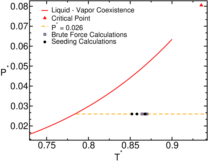
Figure 1: Liquid - Vapor phase diagram of the system under study, taken from Ref. wang2008homogeneous . The isobar for which bubble cavitation has been studied, $P^{*}=0.026$, is indicated with a horizontal dashed line. Black circles correspond to the conditions where seeding simulations were carried out and turquoise squares to brute force simulations of bubble cavitation.

II Simulation details

We carry out computer simulations of the truncated and force-shifted Lennard-Jones (TSF-LJ) potential wang2008homogeneous , a model for which bubble cavitation has been previously studied wang2008homogeneous ; meadley2012thermodynamics ; tanaka2015simple :

$$U_{TSF-LJ}(r)=U_{LJ}(r)-U_{LJ}(r_{c})-(r-r_{c})U^{\prime}_{LJ}(r_{c})$$ (1)

where $U_{LJ}(r)$ is the 12-6 Lennard-Jones potential and $U^{\prime}_{LJ}(r)$ is its first derivative. The interaction potential is truncated and shifted at $r_{c}=2.5\sigma$, being $\sigma$ the particle’s diameter. In what follows, we will use reduced units, expressing all physical variables in terms of $\sigma$, $\epsilon$, the depth of the Lennard-Jones potential, and $m$, the mass of the particles: $T^{*}=k_{B}T\epsilon^{-1}$, $P^{*}=P\cdot\sigma^{3}\epsilon^{-1}$, $\rho^{*}=\rho\cdot\sigma^{3}$ and $t^{*}=t\left(\epsilon m^{-1}\sigma^{-2}\right)^{1/2}$.

All simulations have been performed using the Molecular Dynamics (MD) LAMMPS package lammps_program , applying cubic periodic boundary conditions and integrating the equations of motion with a leap-frog algorithm leapfrog and a timestep of $\Delta t^{*}=0.00046$. Different system sizes have been used to study different bubble sizes: $N=32000$ for the smallest bubble and $N=131072$ for the largest ones (up to a critical radius of 15 $\sigma$). To study bubble nucleation, the system has been equilibrated in an NpT ensemble, whose temperature and pressure are held constant via a Nose-Hover thermostat and barostat JCP_1984_81_00511 with relaxation times $\tau_{T}^{*}=0.46$ and $\tau_{P}^{*}=4.6$ respectively. Our large system sizes allow us to control the pressure with a global barostat despite the fact that the system is heterogeneous marchio2018pressure and to accommodate the bubble in the simulation box without periodic boundary effects. In particular, the ratio between the volume of the system and that of the bubble well exceeds 15 (it ranges from $\sim$ 40 to $\sim$ 100), which is roughly the value beyond which the pressure of a heterogeneous system can be controlled with a global barostat marchio2018pressure .

The pressure-temperature equilibrium phase diagram for the studied model potential is shown in Fig. 1. The solid line is the coexistence line and the black dots the points at which we estimated the bubble nucleation rate with seeding. Bubble nucleation was studied along the $P^{*}=0.026$ isobar, indicated by a horizontal dashed line. Turquoise squares indicate the points at which we estimated the rate by brute force Molecular Dynamics, which was possible due to the high superheating of those state points.

III Seeding of cavitation

According to Classical Nucleation Theory (CNT), the work needed to form a spherical bubble embedded in a metastable liquid at constant pressure and temperature is given by gibbsCNT1 ; gibbsCNT2 ; ZPC_1926_119_277_nolotengo ; becker-doring ; kelton :

$$\Delta G=-V\Delta P+\gamma A_{0},$$ (2)

where $V$ is the volume of the bubble, $\Delta P$ the pressure difference between the bubble and the surrounding liquid, $\gamma$ is the surface tension and $A_{0}$ is the area of the bubble.

For spherical bubbles of radius $R$ the expression above becomes:

$$\Delta G=-\frac{4}{3}\pi R^{3}\Delta P+\gamma 4\pi R^{2}.$$ (3)

By maximizing this function with respect to $R$ the Laplace equation is recovered:

$$R_{c}=\frac{2\gamma}{\Delta P},$$ (4)

where $R_{c}$ is the critical bubble radius. The free energy barrier height corresponding to such radius is:

$$\Delta G_{c}=\frac{2}{3}\pi R_{c}^{3}\Delta P.$$ (5)

Thus, knowing the critical bubble radius and the pressure difference, we can obtain the free energy barrier height.

The bubble nucleation rate, or number of critical bubbles that form per unit time and volume, can be obtained as:

$$J=A\exp(-\Delta G_{c}/k_{B}T),$$ (6)

where $A$ is the kinetic pre-factor, whose calculation is discussed in Section VI.

In the following sections we explain how to compute $R_{c}$, $\Delta P$ and $A$ for a bubble that is critical at $T^{*}=0.852$.

IV Bubble radius

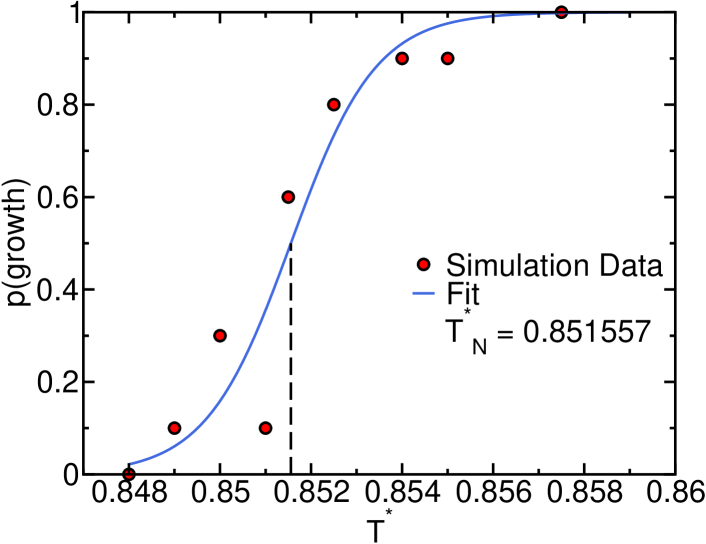
Figure 3: Probability of bubble growth as a function of temperature for a bubble of $R^{ED}=10.5\sigma$

To obtain the critical bubble radius we generate a configuration with a bubble in a superheated fluid from which we launch MD simulations at different temperatures to find the temperature at which the bubble is critical. In the following paragraph we explain how we compute the bubble radius for a given configuration. Let us continue here describing the procedure to generate a bubble configuration and the way we subsequently determine the conditions for which such bubble is critical. In Fig. 2 we summarize the steps followed to obtain an initial bubble configuration. First, we use a spherically symmetric repulsive potential to generate a cavity in the fluid. Once the cavity is generated, the repulsive potential is switched off and a short simulation is then run to allow for the equilibration of the vapor density inside the generated cavity. Finally, we launch several trajectories at different temperatures to obtain the probability that the bubble grows as a function of temperature. The trajectories for T^∗=0.855 are shown in Fig. 2(b) and the data for the probability of bubble growth as a function of temperature are shown in Fig. 3 (red dots). These data are fitted to a sigmoid function (solid line in Fig. 3) and the temperature at which the bubble is critical is that corresponding to a probability of one half. This way of determining the temperature at which the bubble is critical is similar in spirit to the procedure proposed in Ref. sigmoide to deal with finite size effects in establishing coexistence points with the Direct Coexistence method laddCPL1977 ; noyaJCP2008 .

To estimate the bubble’s radius in a given configuration we compute a spherically symmetric density profile from the bubble’s center, $\rho(r)$, as that shown in Fig. 4(a). The bubble center coincides with that of the repulsive particle used to generate it. We have checked that once the repulsive particle is removed the bubble does not move during the time needed to monitor whether the bubble grows or shrinks. In Fig. 4(a) it can be seen that the density is low at short distances, corresponding to the vapor in the interior of the bubble, and high at long distances, corresponding to the liquid. We estimate the radius, $R^{ED}$, as the distance at which the density is the average between that in the interior of the bubble, $\rho_{v}$, and that in the liquid, $\rho_{l}$. We refer to this strategy of finding the bubble radius as the equi-density (ED) method. $\rho_{l}$ and $\rho_{v}$ are obtained by averaging the density far away from and close to the bubble center respectively. This is a rough estimate of the radius because $\rho_{v}$ relies on the first few points of the density profile, which are quite noisy (see Fig. 4(a)). Despite being approximate, this way of obtaining the radius for a single configuration enables to quickly determine whether the bubble grows or shrinks. In this way we have obtained the bubble radius for all points in Fig. 2, for instance.

The radius for the critical bubble, which is the one that is used to estimate the nucleation rate (see Eqs. 5 and 6), is obtained in a more precise manner. First, we collect density profiles of a few critical bubble configurations, which can be obtained in the short period where $R^{ED}$ remains constant before either growing or shrinking at the temperature at which the bubble was found to be critical. Such density profiles for $T^{*}=0.852$ are shown in Fig. 4(b). $\rho_{l}$ can be very accurately determined by averaging the density profiles at distances far away from the bubble center. $\rho_{v}$ is trickier to determine by averaging density profiles due to lack of statistics in the interior of the bubble. Instead, $\rho_{v}$ is obtained by finding the vapor density for which the chemical potential is the same in both phases, a condition that is satisfied only for the critical bubble (this way to obtain $\rho_{v}$ is explained in Section V). Having established $\rho_{l}$ and $\rho_{v}$, we assume a sigmoidal function for $\rho(r)$ and fit the density profile data to the following function:

$$\rho(r)=\frac{\rho_{v}+\rho_{l}}{2}+\left(\frac{\rho_{l}-\rho_{v}}{2}\right)\cdot\tanh\left[(r-R^{ED}_{c})/\alpha\right],$$ (7)

where $\alpha$ is a parameter that is related to the steepness of the interfacial region and $R^{ED}_{c}$ is the radius of the critical bubble for which $\rho(r)=1/2(\rho_{v}+\rho_{l})$, i.e. the equi-density critical radius, which is shown by a vertical orange line in Fig. 4(b). The fit is shown by a solid line in Fig. 4(b). Note that the horizontal part of the fit close to the center, $\rho_{v}$, that was imposed in the fitting procedure to the value obtained by equating the liquid and the vapor chemical potentials, is consistent with the data of the computed density profiles. This is a good consistency test proving that we are actually dealing with the critical bubble in our simulations.

Alternatively, we can define the critical bubble radius according to the equi-molar Gibbs Dividing Surface (GDS) criterion:

$$\int_{0}^{R_{c}^{GDS}}(\rho(r)-\rho_{v})r^{2}dr=\int_{R_{c}^{GDS}}^{\infty}(\rho_{l}-\rho(r))r^{2}dr,$$ (8)

where $R_{c}^{GDS}$ is obtained from the integration limit. To integrate $\rho(r)$ we use the fit previously obtained (Eq. 7). The GDS critical bubble radius is shown by a vertical green line in Fig. 4(b). $R_{c}^{GDS}$ is larger than $R_{c}^{ED}$. Obviously, the computed nucleation rate will depend on which value of the critical radius is used. Later on, in Section VIII, we will discuss which radius yields $J$ values more consistent with independent calculations from the literature.

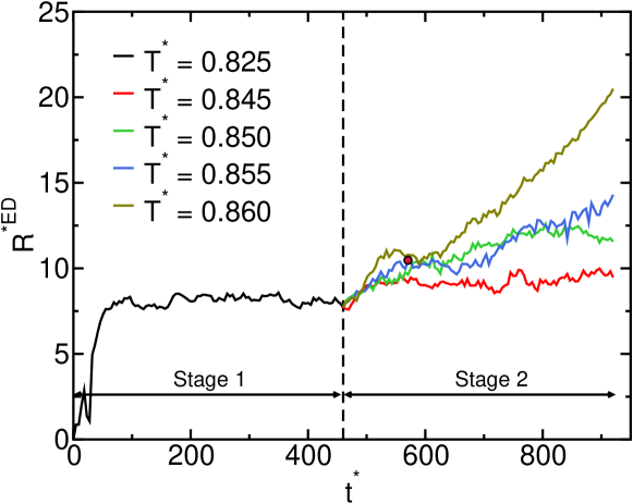
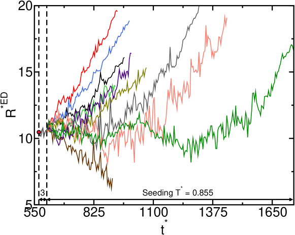
(a) (b)

Figure 2: (a) Bubble radius versus time during the growth of a cavity in a fluid at $P^{*}=0.026$ induced by a spherically repulsive potential with radius of 7.5 $\sigma$ and a height of 0.3 $k_{B}T$. Stage 1: The cavity is grown at a temperature at which the bubble does not grow (black line, $T^{*}=0.825$). Stage 2: With the repulsive potential turned on, the final configuration of Stage 1 is launched at several temperatures to get a first idea of the temperature that makes the grown cavity critical. Trajectories that show immediate growth of the bubble are post-critical (dark green line, $T^{*}=0.860$) whereas those for which the bubble does not grow are pre-critical (red line, $T^{*}=0.845$). We take a configuration from a flat region of a trajectory in between these regimes (blue line, $T^{*}=0.855$) indicated with a red dot in the figure, as a starting point for the next stage. (b) In “stage 3” the repulsive potential is turned off and a short trajectory is launched to ensure that the cavity is filled with an equilibrium vapor density. In the final seeding stage several trajectories (each with a different velocity assignment) starting from the final configuration of stage 3 are launched at the same temperature, $T^{*}=0.855$, to get an estimate of the probability of bubble growth at such temperature (0.9 in this case).

.

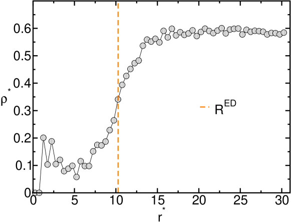
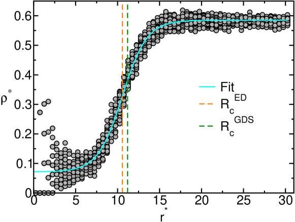
(a) (b)

Figure 4: (a) Radial density as a function of the distance from the bubble centre for a given configuration, and (b) for a set of configurations launched from a critical bubble. Vertical lines indicate the bubble radius according to the ED (dashed orange line) and GDS (dashed green line) criteria.

V Pressure difference

Obtaining $\Delta P$ is a key step in order to estimate both the interfacial free energy and the nucleation rate. $\Delta P$ is the difference between the pressure inside the vapor bubble and the pressure of the metastable liquid around it, i.e. $\Delta P=P^{V}_{N}-P^{L}_{N}$, where the superscripts $V$ and $L$ refer to vapor and liquid respectively, and the subscript $N$ refers to “nucleation”. $P^{L}_{N}$ is simply the pressure imposed in the barostat of our simulations : $p^{*}=0.026$. We have checked that this pressure is also recovered, with less than 1% error, by computing the density in the liquid surrounding the bubble and using the equation of state obtained in independent bulk liquid simulations to obtain the pressure. The pressure inside the bubble can be obtained using the fact that the chemical potential of the liquid and vapor phases is the same both at coexistence conditions, $C$, and when a critical bubble is formed at nucleation conditions. Then, $\mu^{V}_{N}-\mu^{V}_{C}=\mu^{L}_{N}-\mu^{L}_{C}$. These chemical potential differences can be obtained by integrating the volume per molecule, $V_{m}$, from the coexistence pressure, $P_{C}$, to the nucleation one, $P_{N}$, at the temperature at which we found that the inserted bubble is critical:

$$\int_{P_{C}}^{P^{L}_{N}}V^{L}_{m}dP=\int_{P_{C}}^{P^{V}_{N}}V^{V}_{m}dP$$ (9)

$V_{m}$ as a function of pressure can be easily obtained in simulations of the pure liquid and vapor phases. The only unknown in the equation above is the upper integration limit of the right-hand-side integral, $P^{V}_{N}$, which is what we need to obtain $\Delta P$. We obtained for our case study $\Delta P^{*}=0.0163$. Note that once $P^{V}_{N}$ is known, it is immediate to obtain $\rho_{v}$ from the equation of state, which is needed to estimate the critical bubble radius according to Eqs. 7 and 8.

Moreover, repeating this procedure along the isobar, we observe a linear tendency of $\Delta P$ as a function of the temperature, as shown in figure 5. As discussed later, this linear dependence will be used to fit the nucleation rate as a function of temperature.

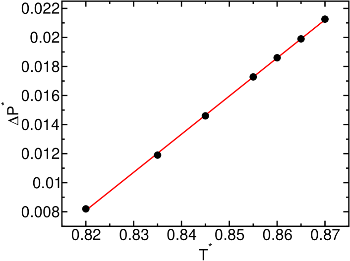
Figure 5: Pressure difference between the inside of the bubble and the surrounding liquid, $\Delta P$ as a function of the temperature for the isobar $P^{*}=0.026$. Black dots correspond to data obtained integrating Eq. 9 for each temperature and the linear fit for this data, shown in red, is $\Delta P^{*}=-0.2071+0.2624\cdot T^{*}$.

VI Kinetic pre-factor

The kinetic prefactor for bubble nucleation is often computed as suggested in Blanderino :

$$A=\rho_{l}\sqrt{\frac{\Delta PR_{c}}{\pi m}},$$ (10)

$m$ being the particle mass and $\rho_{l}$ the number density of the fluid. Therefore, we can obtain the kinetic pre-factor with the information we have already computed: $R_{c}$ and $\Delta P$.

For our case study, $P^{*}=0.026$ and $T^{*}=0.852$, this equation gives a value for the kinetic pre-factor of $A^{*}=0.139$.

A second route to compute the kinetic pre-factor is given in Ref. menzl2016molecular :

$$A=\frac{\sqrt{k_{B}T\Delta P(R_{c}/2)^{3}}}{\eta}\rho_{l}\rho_{v},$$ (11)

where $\eta$ is the viscosity of the metastable liquid, $\eta^{*}=0.737$ in our case, and $\rho_{l}$ and $\rho_{v}$ are the number density of liquid and vapor respectively. The kinetic pre-factor thus obtained is $A^{*}=0.07$.

Alternatively, we have adapted the expression proposed by Frenkel and Auer for the kinetic pre-factor for crystal nucleation Nature_2001_409_1020 ; auerJCP2004 to our problem of bubble nucleation. Auer and Frenkel proposed that the kinetic pre-factor can be obtained via:

$$A=\rho_{l}\cdot Z\cdot f^{+},$$ (12)

where $Z$, the Zeldovich factor, is given by kelton ; ZPC_1926_119_277_nolotengo ; becker-doring :

$$Z=\sqrt{\frac{\Delta P}{8\pi^{2}k_{B}T\rho_{v}^{2}\cdot R_{c}^{3}}},$$ (13)

$\rho_{v}$ being the number density of vapor particles inside the bubble, obtained from the equation of state once we know the pressure inside the bubble from the integration of the molecular volumes from coexistence to nucleation conditions, Eq. 9. $f^{+}$, is the attachment rate, that can be computed from the expression proposed by Auer and Frenkel Nature_2001_409_1020 ; auerJCP2004 :

$$f^{+}=\frac{\left\langle\left(N_{v}(t)-N_{v}(0)\right)^{2}\right\rangle}{2t},$$ (14)

where $N_{v}$ is the number of vapor particles in the bubble. To estimate $f^{+}$ according to this equation we monitor the bubble radius as a function of time, $R(t)$ (see IV), for dozens of molecular dynamics trajectories originated at the critical bubble. Figure 6(a) shows $R(t)$ for our case study. The fact that the bubble grows/shrinks in half of the trajectories proofs that we are indeed dealing with a critical bubble. We can easily convert the bubble radius to $N_{v}$ assuming a spherical bubble shape and knowing the vapor density in the critical bubble, $\rho_{v}$. We obtain the latter from $P^{N}_{V}$ (see Eq. 9) and the vapor equation of state. From such trajectories one can easily obtain the average of the equation above, as shown in Fig. 6(b). The kinetic pre-factor obtained from the slope of Fig. 6(b) and Eq. 12 is $A^{*}=0.09$. This approach by Auer and Frenkel to compute the kinetic pre-factor has been used so far for the nucleation of crystals. Here, we use it for the first time for vapor nucleation. The good agreement between this approach and the other two previously discussed in this section suggests that it is reasonable to assume, as Auer and Frenkel did for crystal nucleation, that the growth of the vapor bubble occurs by attachment of vapor particles. This view needs to be confirmed with a more careful theoretical treatment, a task that goes beyond the scope of our work. Here, we are satisfied with the fact that the kinetic pre-factors obtained from Eqs. 10, 11 and 12 are of the same order of magnitude (0.139, 0.07 and 0.09 respectively), which is quite satisfactory for the calculation of nucleation rates. We note that these values were computed for $R_{c}=R_{c}^{ED}$. If the GDS radius definition had been used instead, the values would be slightly different, but within the same order of magnitude. It may seem surprising that all three expressions for the rate give similar values in view of the fact that they have different dependences on the vapor density, $\rho_{v}$. However, as reported in Table 1, the vapor density does not change much from one bubble to another.

Since all three routes to estimate $A$ yield results within the same order of magnitude we can choose the handiest one for the calculation of the nucleation rate (Section VIII). Accordingly, we shall use Eq. 10, that only depends on $R_{c}$, $\Delta P$ and $\rho_{l}$. The other expressions require costly calculations either of the viscosity (Eq. 11) or of the attachment rate (Eq. 12). Moreover, Eq. 10, combined with the Laplace equation, gives $A=\rho_{l}\sqrt{2\gamma/(\pi m)}$, that only depends on $\rho_{l}$ and $\gamma$. As we show in the following section, $\gamma$ varies linearly with temperature. Therefore, $A$ can easily be obtained at any temperature in order to fit the seeding data for the nucleation rate (see Section VIII).

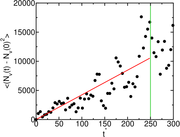
(a) (b)

Figure 6: (a): Time evolution of the critical bubble radius for 10 trajectories launched with different momenta initialization starting from a critical bubble at $P^{*}=0.026$ and $T^{*}=0.852$. (b): Squared deviation of the number of particles in the vapor bubble, $N_{v}$ with respect to its initial value averaged over the 10 trajectories shown in panel (a). The slope of a linear fit for the first $250t^{*}$ (red line) gives the attachment rate, $f^{+}$.

$N$	$R_{c}^{ED}$	$R_{c}^{GDS}$	$T$	$\Delta P$	$\gamma_{ED}$	$\gamma_{GDS}$	$\rho_{v}$	$A_{ED}$	$A_{GDS}$	$\log(J_{ED})$	$\log(J_{GDS})$
32000	5.40	6.98	0.868	0.0207	0.053	0.068	0.0786	0.105	0.119	-4.2	-7.9
131072	7.93	9.06	0.858	0.0182	0.069	0.078	0.0728	0.125	0.133	-10.0	-14.5
131072	10.5	11.19	0.852	0.0163	0.082	0.087	0.0715	0.139	0.144	-20.1	-24.2

Table 1: Data for the bubble seeding simulations performed in this work at $P^{*}=0.026$ (in reduced LJ units). We report the number or particles in the simulation box, $N$, the bubble radii obtained with two different criteria, $R_{c}^{ED}$ and $R_{c}^{GDS}$, the temperature at which the bubble is found to be critical, $T$, the pressure difference between the bubble and the surrounding liquid, $\Delta P$, the surface tension obtained with the same two criteria, $\gamma_{ED}$ and $\gamma_{GDS}$, the vapor density inside the bubble, $\rho_{v}$, the kinetic pre-factor as obtained from Eq. 10 also for two different criteria, $A_{ED}$ and $A_{GDS}$ and the nucleation rates corresponding to each criterion to determine the bubble radius, $\log(J_{ED})$ and $\log(J_{GDS})$. All variables are given in reduced units.

VII Surface tension

We can use the Laplace equation (Eq. 4) to obtain $\gamma$ from $R_{c}$ and $\Delta P$. The data thus obtained for each bubble are shown in Fig. 7. There are three sets of data: orange and green, corresponding to the ED and GDS definition of the critical bubble radius respectively. $R_{c}^{ED}$ is lower than $R_{c}^{GDS}$ and therefore, according to Laplace equation, yields lower values of $\gamma$. These two sets can be compared to the third, the pink, corresponding to the surface of tension at the coexistence pressure for each temperature (reported in Table 2). This is obtained performing NVT molecular dynamics simulations of a liquid and a vapor at coexistence, where the pressure tensor is calculated once the system has equilibrated following the Irving-Kirkwood expression walton1983pressure :

$$\gamma=\frac{L_{z}}{2}(\bar{P}_{z}-\bar{P}_{x,y})$$ (15)

where $z$ is the direction perpendicular to the liquid-vapor planar interfase and $x$ and $y$ are the tangential directions to the interface. As shown in Fig. 7, $\gamma_{Coex}$ is higher than that obtained in our seeding simulations. The coexistence temperature at the pressure at which all calculations have been performed in this work, $P^{*}=0.026$, is indicated by a vertical dashed line in the figure ($T^{*}=0.781$). A linear extrapolation of the $\gamma$ seeding data to the coexistence temperature is consistent with the surface tension at coexistence ($\gamma^{*}_{Coex}=0.21$).

Our results in Fig. 7 show that $\gamma$ goes down as the liquid becomes superheated at constant pressure or undercompressed at constant temperature. Accordingly, both routes to obtain a metastable liquid are associated with a positive Tolman length tolman1949effect ; rowlinson2013molecular , $\delta$, in the following expression to describe the variation of $\gamma$ with the critical bubble radius: $\gamma=\gamma_{Coex}\left(1-\frac{2\delta}{R_{c}}\right)$, montero2019interfacial . It is also clear from Fig. 7 that the variation of $\gamma$ with pressure at constant temperature is milder than that with temperature at constant pressure. Also for the crystal-liquid interface $\gamma$ changes as the system gets away from coexistence seedingvienes ; espinosaPRL2016 ; montero2019interfacial .

$T^{*}$	0.781	0.785	0.8	0.81	0.82	0.83	0.84	0.85	0.86
$\gamma_{Coex}^{*}$	0.205	0.193	0.176	0.164	0.145	0.144	0.123	0.102	0.096

Table 2: Surface tension at coexistence as a function of the temperature. Obtained from long coexistence runs and applying Eq. 15.

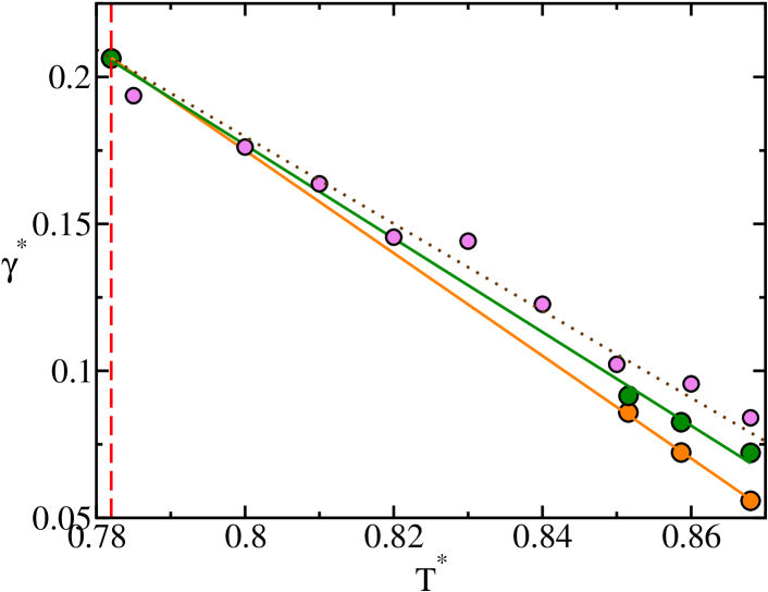
Figure 7: Surface tension as a function of temperature at $P^{*}=0.026$. Orange and green symbols correspond to the ED and GDS definitions of the critical bubble radius respectively. Orange and green lines are linear fits to the corresponding data. Pink symbols correspond to data obtained from direct coexistence simulations, $\gamma_{Coex}$, and the dotted line corresponds to a linear fit to these data: $\gamma_{Coex}^{*}=1.3644-1.4809\cdot T^{*}$.

VIII Nucleation Rate

With data for the bubble critical radius, the pressure difference between the fluid and the interior of the bubble and the kinetic pre-factor, we obtain the nucleation rate as explained in Sec. III. In Table 1 we provide the values of these parameters for the three bubble sizes considered in this work. As justified in Section VI, the kinetic pre-factor used to compute the rate and reported in Table 1 has been computed by means of Eq. 10. Two different rates are obtained, one for the equi-density definition of the bubble radius, $J_{ED}$, and another for the Gibbs Dividing surface definition, $J_{GDS}$. The results for the rates thus obtained are shown with dots in Fig. 8. Orange and green symbols correspond to $J_{ED}$ and $J_{GDS}$ respectively. The values for the latter are lower because $R^{GDS}_{c}$ is larger than $R^{ED}_{c}$ (see Fig. 4(b) and table 1) and, according to Eq. 5, a larger radius gives raise to a higher Gibbs free energy barrier and, therefore, to a lower rate. As critical bubbles become larger (or the superheating decreases) the difference between both radii decreases.

We now fit the seeding data of $J(T)$ to a curve inspired on the CNT expressions used to compute the nucleation rate. By combining Eqs. 4, 5 and 10 the rate can be expressed only in terms of $\gamma$, $\Delta P$ and $\rho_{l}$. The temperature dependence of the latter is trivially obtained from the equation of state, for that of $\gamma$ we use the linear fits shown in Fig. 7 and for $\Delta P(T)$ that shown in 5. Thus, we obtain the solid orange and green curves in Fig. 8 that describe the variation of the nucleation rate with temperature. The dashed lines indicate the error bars for each $J$ curve, obtained assuming a 0.3 $\sigma$ error in the determination of the radius. The 0.3 $\sigma$ error comes, on the one hand, from the statistical uncertainty in the determination of the radius for a given temperature and, on the other hand, from the uncertainty related with the determination of the temperature itself in the seeding simulations. Other error sources like $\Delta P$, which is obtained by integrating highly accurate equations of state, or the kinetic pre-factor, for which similar values are obtained via three different approaches (see VI), yield a negligible contribution to the rate error as compared to that of the radius. The red curve in Fig. 8 is obtained using the coexistence, $\gamma_{Coex}$ for each temperature instead of the $\gamma$ coming from seeding. We have already shown in Fig. 7 that, for a given temperature, the coexistence $\gamma$ is higher than that obtained from seeding. Accordingly, the rate curve coming from the coexistence $\gamma$ (in red in Fig. 8) is lower that those coming from seeding (green and orange curves). This means that the capillary approximation –using $\gamma_{Coex}$ in CNT– is not valid to obtain nucleation rates.

The difference between both seeding curves, $J_{GDS}$ and $J_{ED}$, reflects the ambiguity of the seeding technique with regards to the employed criterion to determine the size of the critical nucleus espinosaJCP2016_2 . The question is, what is the right value for the radius, $R_{c}^{ED}$ or $R_{c}^{GDS}$? The answer is neither, because the correct radius is the one that provides the correct value for the nucleation rate. That radius should correspond to the surface of tension, defined as the radius for which Laplace equation holds rowlinson2013molecular (recall from Section III that the Laplace equation is naturally derived from the CNT formalism behind the seeding technique). Unfortunately, there is no way to determine the radius of tension from our seeding simulations since this would require the determination of the free energy of the system (i.e there is no rigorous mechanical route to the radius of the surface of tension) rowlinson2013molecular .

Therefore, we operationally chose the definition of $R_{c}$ that gives values of $J$ closer to those obtained with techniques that do not depend on CNT. In Fig. 8 we show with black and red symbols the values obtained in Refs. meadley2012thermodynamics ; wang2008homogeneous for a given state point, $T^{*}=0.855$ and $P^{*}=0.026$, with rare event techniques like Forward Flux Sampling PRL_2005_94_018104 or Umbrella Sampling JCP_1992_96_04655 . These literature values are in better agreement with the seeding fit obtained with the ED definition of $R_{c}$. Therefore, it seems from this comparison that $R_{c}^{ED}$ gives the correct $J$ (i. e. that the surface of tension is closer to the ED than to the GDS).

However, this conclusion is contradictory with that drawn from comparing seeding data with those obtained from spontaneous cavitation at large superheating. In such conditions the formation of a critical bubble is spontaneous and the rate can be computed as filion:244115 :

$$J=\frac{1}{<t>V}$$ (16)

where $<t>$ is the average time required to observe cavitation, which is detected by a sudden density drop. In Fig. 9 we show the density as a function of time for several trajectories at $T^{*}=0.87$ and $P^{*}=0.026$. The stochastic nature of the formation of a critical bubble is evident from the dispersion of cavitation times in the figure. In this way we have computed the nucleation rate for several state points at large superheating. The results are shown with salmon diamonds in Fig. 8 and are reported in table 3.

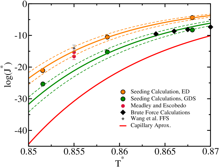
Figure 8: Bubble nucleation rate for $P^{*}=0.026$ as a function of temperature. Orange and green dots are seeding results from this work with $R_{c}^{ED}$ and $R_{c}^{GDS}$ respectively. Solid orange and green lines are CNT-inspired fits to the seeding data. Dashed orange and green curves indicate the error bars. Red dots meadley2012thermodynamics and black diamond wang2008homogeneous are literature values. Salmon diamonds are results from this work obtained at large superheating by spontaneous cavitation (brute force molecular dynamics). The red curve corresponds to the capillary approximation, where the coexistence $\gamma$ for each temperature has been used to estimate the nucleation rate via Eqs. 4, 5, 6 and 10.

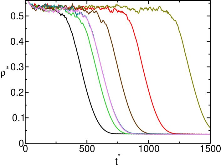
Figure 9: Total density of the system versus time for several trajectories starting from an equilibrated fluid at $T^{*}=0.87$ and $P^{*}=0.026$.

$T^{*}$	0.8640	0.8660	0.8675	0.8700
$log(J^{*})$	-9.53	-8.66	-8.14	-7.35

Table 3: Brute Force calculations of the nucleation rate at different temperatures and $P^{*}=0.026$.

Somewhat frustratingly, the seeding curve that better agrees with the spontaneous cavitation data is that coming from the GDS definition of the critical bubble radius. This means that the surface of tension, that would provide the true value for the nucleation rate, is neither provided by the ED nor the GDS. Therefore, there is no single seeding curve able to describe the nucleation rate in the whole temperature range. The ED curve works better for moderate superheating, whereas the GDS one is more accurate at large superheating. It is worth recalling here that seeding is expected to work better for large bubbles (small superheating) given that it relies on the CNT assumption that the bubble has thermodynamic entity. In this respect, the radius that reproduces the data at low superheating, $R^{ED}$, is the most reliable for making seeding estimates of the nucleation rate. $R^{GDS}$ is not so useful then. After all, at large superheating, where bubble cavitation is spontaneous, there is no need for seeding predictions. . In any case it is worth noting that seeding is an approximate technique whose strength is its ability to provide values of the rate for a large range of orders of magnitude, at the expense of accuracy. In this respect, $R^{ED}$ yields reasonably good results in the whole temperature range. In fact, the difference between seeding and spontaneous nucleation data is of the same order of magnitude as that previously found in seeding studies of crystallization seedingvienes .

IX Summary and conclusions

We investigate bubble cavitation in a superheated Lennard Jones fluid with computer simulations using the Seeding method. We prepare configurations of a fluid at $P^{*}=0.026$ containing a vapor bubble, and launch several Molecular Dynamics trajectories at different temperatures to find that at which the generated bubble is critical (i. e. it has a growth chance of 1/2). We calculate the bubble radius with the aid of radial density profiles centred at the bubble and the pressure inside the bubbles with thermodynamic integration assuming that the chemical potential of the vapor and the liquid is the same for the critical bubble. With this information we estimate the free energy required to form the critical bubble via Classical Nucleation Theory. The exponential of such barrier combined with a kinetic pre-factor, that we obtain with three different approaches consistent among themselves, gives us an estimate of the bubble nucleation rate. The seeding nucleation rate is in fairly good agreement with independent calculations using techniques that do not depend on Classical Nucleation Theory. We use two different ways of identifying the bubble radius. One based on the point at which the density is the average between that of the vapor and of the liquid, and another based on the equi-molar Gibbs dividing surface. We conclude that the density based radius definition is more reliable for making seeding predictions because it works better in the regime where CNT assumptions, on which seeding relies, are more justifiable. Our simulations show that using the surface tension at coexistence for a given temperature to estimate nucleation rates does not give good results because the surface tension varies with pressure for a given temperature (or with temperature for a given pressure). Therefore, seeding simulations are needed to get reasonable nucleation rates in combination with Classical Nucleation Theory. Finally, we note that the seeding technique is quite powerful: working with three different bubble sizes we were able to estimate nucleation rates in a range of tens of orders of magnitude.

X Acknowledgments

This work was funded by grant FIS2016/78117-P of the MEC. C. Valeriani thanks financial support from FIS2016-78847-P of the MEC. The authors acknowledge the computer resources and technical assistance provided by the RES and L. G. MacDowell for useful discussions.

References

- (1) M. Shusser and D. Weihs, “Explosive boiling of a liquid droplet,” International journal of multiphase flow, vol. 25, no. 8, pp. 1561–1573, 1999.
- (2) M. Shusser, T. Ytrehus, and D. Weihs, “Kinetic theory analysis of explosive boiling of a liquid droplet,” Fluid Dynamics Research, vol. 27, no. 6, p. 353, 2000.
- (3) A. Toramaru, “Vesiculation process and bubble size distributions in ascending magmas with constant velocities,” Journal of Geophysical Research: Solid Earth, vol. 94, no. B12, pp. 17523–17542, 1989.
- (4) H. Massol and T. Koyaguchi, “The effect of magma flow on nucleation of gas bubbles in a volcanic conduit,” Journal of volcanology and geothermal research, vol. 143, no. 1-3, pp. 69–88, 2005.
- (5) C. E. Brennen, Cavitation and bubble dynamics. Cambridge University Press, 2014.
- (6) K. S. Suslick, “Sonochemistry,” science, vol. 247, no. 4949, pp. 1439–1445, 1990.
- (7) K. S. Suslick, M. M. Mdleleni, and J. T. Ries, “Chemistry induced by hydrodynamic cavitation,” Journal of the American Chemical Society, vol. 119, no. 39, pp. 9303–9304, 1997.
- (8) Z.-J. Wang, C. Valeriani, and D. Frenkel, “Homogeneous bubble nucleation driven by local hot spots: A molecular dynamics study,” The Journal of Physical Chemistry B, vol. 113, no. 12, pp. 3776–3784, 2008.
- (9) S. L. Meadley and F. A. Escobedo, “Thermodynamics and kinetics of bubble nucleation: Simulation methodology,” The Journal of chemical physics, vol. 137, no. 7, p. 074109, 2012.
- (10) K. K. Tanaka, H. Tanaka, R. Angelil, and J. Diemand, “Simple improvements to classical bubble nucleation models,” Physical review E, vol. 92, no. 2, p. 022401, 2015.
- (11) G. Menzl, M. A. Gonzalez, P. Geiger, F. Caupin, J. L. Abascal, C. Valeriani, and C. Dellago, “Molecular mechanism for cavitation in water under tension,” Proceedings of the National Academy of Sciences, vol. 113, no. 48, pp. 13582–13587, 2016.
- (12) R. P. Sear, “Nucleation: theory and applications to protein solutions and colloidal suspensions,” Journal of Physics: Condensed Matter, vol. 19, no. 3, p. 033101, 2007.
- (13) G. C. Sosso, J. Chen, S. J. Cox, M. Fitzner, P. Pedevilla, A. Zen, and A. Michaelides, “Crystal nucleation in liquids: Open questions and future challenges in molecular dynamics simulations,” Chemical Reviews, vol. 116, no. 12, pp. 7078–7116, 2016.
- (14) A. V. Brukhno, J. Anwar, R. Davidchack, and R. Handel, “Challenges in molecular simulation of homogeneous ice nucleation,” Journal of Physics: Condensed Matter, vol. 20, no. 49, p. 494243, 2008.
- (15) P. R. ten Wolde and D. Frenkel, “Computer simulation study of gas-liquid nucleation in a Lennard-Jones system,” J. Chem. Phys., vol. 109, p. 9901, 1998.
- (16) C. Valeriani, E. Sanz, and D. Frenkel, “Rate of homogeneous crystal nucleation in molten NaCl,” J. Chem. Phys., vol. 122, p. 194501, 2005.
- (17) J. S. van Duijneveld and D. Frenkel, “Computer simulation study of free energy barriers in crystal nucleation,” J. Chem. Phys., vol. 96, p. 4655, 1992.
- (18) A. Haji-Akbari and P. G. Debenedetti, “Direct calculation of ice homogeneous nucleation rate for a molecular model of water,” Proceedings of the National Academy of Sciences, vol. 112, no. 34, pp. 10582–10588, 2015.
- (19) H. Jiang, A. Haji-Akbari, P. G. Debenedetti, and A. Z. Panagiotopoulos, “Forward flux sampling calculation of homogeneous nucleation rates from aqueous nacl solutions,” The Journal of Chemical Physics, vol. 148, no. 4, p. 044505, 2018.
- (20) K. F. Kelton, Crystal Nucleation in Liquids and Glasses. Boston: Academic, 1991.
- (21) M. Volmer and A. Weber, “Keimbildung in ubersattigten gebilden,” Z. Phys. Chem., vol. 119, p. 277, 1926.
- (22) R. Becker and W. Doring, “Kinetische behandlung der keimbildung in ubersattigten dampfen,” Ann. Phys., vol. 416, pp. 719–752, 1935.
- (23) J. R. Espinosa, C. Vega, C. Valeriani, and E. Sanz, “Seeding approach to crystal nucleation,” J. Chem. Phys., vol. 144, p. 034501, 2016.
- (24) E. Sanz, C. Vega, J. R. Espinosa, R. Caballero-Bernal, J. L. F. Abascal, and C. Valeriani, “Homogeneous ice nucleation at moderate supercooling from molecular simulation,” Journal of the American Chemical Society, vol. 135, no. 40, pp. 15008–15017, 2013.
- (25) A. Zaragoza, M. M. Conde, J. R. Espinosa, C. Valeriani, C. Vega, and E. Sanz, “Competition between ices ih and ic in homogeneous water freezing,” The Journal of Chemical Physics, vol. 143, no. 13, p. 134504, 2015.
- (26) J. R. Espinosa, A. Zaragoza, P. Rosales-Pelaez, C. Navarro, C. Valeriani, C. Vega, and E. Sanz, “Interfacial free energy as the key to the pressure-induced deceleration of ice nucleation,” Phys. Rev. Lett., vol. 117, p. 135702, 2016.
- (27) S. Plimpton J. Comput. Phys., vol. 117, p. 1, 1995.
- (28) R. W. Hockney, S. P. Goel, and J. Eastwood, “Quiet high resolution computer models of a plasma,” J. Comp. Phys., vol. 14, pp. 148–158, 1974.
- (29) S. Nosé, “A unified formulation of the constant temperature molecular dynamics methods,” J. Chem. Phys., vol. 81, p. 511, 1984.
- (30) S. Marchio, S. Meloni, A. Giacomello, C. Valeriani, and C. Casciola, “Pressure control in interfacial systems: Atomistic simulations of vapor nucleation,” The Journal of chemical physics, vol. 148, no. 6, p. 064706, 2018.
- (31) J. W. Gibbs, “On the equilibrium of heterogeneous substances,” Trans. Connect. Acad. Sci., vol. 3, pp. 108–248, 1876.
- (32) J. W. Gibbs, “On the equilibrium of heterogeneous substances,” Trans. Connect. Acad. Sci., vol. 16, pp. 343–524, 1878.
- (33) J. R. Espinosa, E. Sanz, C. Valeriani, and C. Vega, “On fluid-solid direct coexistence simulations: The pseudo-hard sphere model,” The Journal of Chemical Physics, vol. 139, no. 14, p. 144502, 2013.
- (34) A. Ladd and L. Woodcock, “Triple-point coexistence properties of the lennard-jones system,” Chemical Physics Letters, vol. 51, no. 1, pp. 155 – 159, 1977.
- (35) E. G. Noya, C. Vega, and E. de Miguel, “Determination of the melting point of hard spheres from direct coexistence simulation methods,” The Journal of Chemical Physics, vol. 128, no. 15, p. 154507, 2008.
- (36) Blander, Milton, and Joseph L. Katz. , “Bubble nucleation in liquids.,” AIChE Journal, vol. 21.5, pp. 33–848, 1975.
- (37) S. Auer and D. Frenkel, “Prediction of absolute crystal-nucleation rate in hard-sphere colloids,” Nature, vol. 409, p. 1020, 2001.
- (38) S. Auer and D. Frenkel, “Numerical prediction of absolute crystallization rates in hard-sphere colloids,” J. Phys.:Condens. Matter, vol. 120, p. 3015, 2004.
- (39) J. Walton, D. Tildesley, J. Rowlinson, and J. Henderson, “The pressure tensor at the planar surface of a liquid,” Molecular physics, vol. 48, no. 6, pp. 1357–1368, 1983.
- (40) R. C. Tolman, “The effect of droplet size on surface tension,” The journal of chemical physics, vol. 17, no. 3, pp. 333–337, 1949.
- (41) J. S. Rowlinson and B. Widom, Molecular theory of capillarity. Courier Corporation, 2013.
- (42) P. Montero de Hijes, J. R. Espinosa, E. Sanz, and C. Vega, “Interfacial free energy of a liquid-solid interface: Its change with curvature,” The Journal of Chemical Physics, vol. 151, no. 14, p. 144501, 2019.
- (43) J. R. Espinosa, J. M. Young, H. Jiang, D. Gupta, C. Vega, E. Sanz, P. G. Debenedetti, and A. Z. Panagiotopoulos, “On the calculation of solubilities via direct coexistence simulations: Investigation of nacl aqueous solutions and lennard-jones binary mixtures,” The Journal of Chemical Physics, vol. 145, no. 15, p. 154111, 2016.
- (44) R. J. Allen, P. B. Warren, and P. R. ten Wolde, “Sampling rare switching events in biochemical networks,” Phys. Rev. Lett., vol. 94, p. 018104, 2005.
- (45) J. S. van Duijneveldt and D. Frenkel, “Computer simulation study of free energy barriers in crystal nucleation,” J. Chem. Phys., vol. 96, p. 4655, 1992.
- (46) L. Filion, M. Hermes, R. Ni, and M. Dijkstra, “Crystal nucleation of hard spheres using molecular dynamics, umbrella sampling, and forward flux sampling: A comparison of simulation techniques,” J. Chem. Phys., vol. 133, no. 24, p. 244115, 2010.