On the Linear Convergence Rate
of the Distributed Block Proximal Method

Abstract

The recently developed Distributed Block Proximal Method, for solving stochastic big-data convex optimization problems, is studied in this paper under the assumption of constant stepsizes and strongly convex (possibly non-smooth) local objective functions. This class of problems arises in many learning and classification problems in which, for example, strongly-convex regularizing functions are included in the objective function, the decision variable is extremely high dimensional, and large datasets are employed. The algorithm produces local estimates by means of block-wise updates and communication among the agents. The expected distance from the (global) optimum, in terms of cost value, is shown to decay linearly to a constant value which is proportional to the selected local stepsizes. A numerical example involving a classification problem corroborates the theoretical results.

1 Introduction

In this paper, we address in a distributed way stochastic big-data convex optimization problems involving strongly convex (possibly nonsmooth) local objective functions, by means of the Distributed Block Proximal Method [1, 2]. Problems with this structure naturally arise in many learning and control problems in which the decision variable is extremely high dimensional and large datasets are employed. Relevant examples include: direct policy search in reinforcement learning [3], dynamic problems involving stochastic functions generated from collected samples to be processed online [4], learning problems involving massive datasets in which sample average approximation techniques are used [5], and settings in which only noisy subgradients of the objective functions can be computed at each time instant [6].

Distributed algorithms for solving stochastic problems have been widely studied [6, 7, 8, 9, 10, 11]. On the other side, distributed algorithms for big-data problems through block communication have started to appear only recently [12, 13, 14, 15, 16]. The Distributed Block Proximal Method solves problems that can be together non-smooth, stochastic and big-data, thus distinguishing from the above works (see [1] for a comprehensive literature review). This algorithm evolves through block-wise communication and updates (involving subgradients of the local functions and proximal mappings induced by some distance genereting functions) and it has been already shown to achieve a sublinear convergence rate on problems with non-smooth convex objective functions. The contribution of this paper is to extend this result by showing that, under strongly convex (possibly non-smooth) local objective functions and constant stepsizes, the Distributed Block Proximal Method exhibits a linear convergence rate (with a constant error term) to the optimal cost in expected value. The main challenge in the linear-rate analysis relies in the block-wise nature of the algorithm.

2 Set-up and preliminaries

2.1 Notation, definitions and preliminary results

Given a vector $x\in\mathbb{R}^{n}$, we denote by $x_{\ell}$ the $\ell$-th block of $x$, i.e., given a partition of the identity matrix $I=[U_{1},\dots,U_{B}]$, with $U_{\ell}\in\mathbb{R}^{n\times n_{\ell}}$ for all $\ell$ and $\sum_{\ell=1}^{B}n_{\ell}=n$, it holds $x=\sum_{\ell=1}^{B}U_{\ell}x_{\ell}$ and $x_{\ell}=(U_{\ell})^{\top}x$. In general, given a vector $x_{i}\in\mathbb{R}^{n}$, we denote by $x_{i,\ell}$ the $\ell$-th block of $x_{i}$. Given a matrix $A$, we denote by $a_{ij}$ the element of $A$ located at row $i$ and column $j$. Given two vectors $a,b\in\mathbb{R}^{n}$ we denote by $\langle a,b\rangle$ their scalar product. Given a discrete random variable $r\in\{1,\ldots,R\}$, we denote by $P(r=\bar{r})$ the probability of $r$ to be equal to $\bar{r}$ for all $\bar{r}\in\{1,\ldots,R\}$. Given a nonsmooth function $f$, we denote by $\partial f(x)$ its subdifferential at $x$.

The following preliminary result will be used in the paper.

Lemma 1.

Given any two scalars $\delta\neq\gamma\neq 1$, it holds that

1. $\sum_{s=r}^{t}\delta^{s}=\frac{\delta^{r}-\delta^{t+1}}{1-\delta}$

2. $\sum_{s=0}^{t}\delta^{t-s}\gamma^{s}=\frac{\delta^{t+1}-\gamma^{t+1}}{\delta-\gamma}.$ $\square$

2.2 Distributed stochastic optimization set-up

Let us start by formalizing the optimization problem addressed in this paper. We consider problems in the form

$$\mathop{\textrm{minimize}}_{x\in X} \sum_{i=1}^{N}\mathbb{E}[h_{i}(x;\xi_{i})].$$ (1)

where $\xi_{i}$ is a random variable and $x\in\mathbb{R}^{n}$, $n\gg 1$, has a block structure, i.e., $x=[x_{1}^{\top},\dots,x_{B}^{\top}]^{\top}.$, with $x_{\ell}\in\mathbb{R}^{n_{\ell}}$ for all $\ell$ and $\sum_{\ell=1}^{B}n_{\ell}=n$. The decision variable $x$ can be very high-dimensional, which calls for block-wise algorithms.

Let $f_{i}(x)\triangleq\mathbb{E}[h_{i}(x;\xi_{i})]$. Moreover, let $g_{i}(x;\xi_{i})\in\partial h_{i}(x;\xi_{i})$ (resp. $\textsl{g}_{i}(x)\in\partial f_{i}(x)$) be a subgradient of $h_{i}(x;\xi_{i})$ (resp. $f_{i}(x)$) computed at $x$. Then, the following assumption holds for problem (1).

Assumption 1 (Problem structure).

1. The constraint set $X$ has the block structure $X=X_{1}\times\dots\times X_{B}$, where, for $\ell=1,\dots,B$, the set $X_{\ell}\subseteq\mathbb{R}^{n_{\ell}}$ is closed and convex, and $\sum_{\ell=1}^{B}n_{\ell}=n$.

2. The function $h_{i}(x,\xi_{i}):\mathbb{R}^{n}\to\mathbb{R}$ is continuous, strongly convex and possibly nonsmooth for all $x\in X$ and every $\xi_{i}$, for all $i\in\{1,\ldots,N\}$. In particular, there exists a constant $m>0$ such that $f_{i}(a)\geq f_{i}(b)-\langle\textsl{g}_{i}(b),b-a\rangle+\frac{m}{2}\|a-b\|^{2}$, for all $a,b\in X$ and all $i\in\{1,\ldots,N\}$.

3. every subgradient $g_{i}(x;\xi_{i})$ is an unbiased estimator of the subgradient of $f_{i}$, i.e., $\mathbb{E}[g_{i}(x;\xi_{i})]=\textsl{g}_{i}(x)$. Moreover, there exist constants $G_{i}\in[0,\infty)$ and $\bar{G}_{i}\in[0,\infty)$ such that $\mathbb{E}[\|g_{i}(x;\xi_{i})\|]\leq G_{i}$, and $\mathbb{E}[\|g_{i}(x;\xi_{i})\|^{2}]\leq\bar{G}_{i}$, for all $x$ and $\xi_{i}$, for all $i\in\{1,\ldots,N\}$. $\square$

Let us denote by $g_{i,\ell}(x;\xi_{i})$ the $\ell$-th block of $g_{i}(x;\xi_{i})$ and let $\textsl{g}(x)\in\partial f(x)$ be a subgradient of $f$ computed at $x$. Then, Assumption 1(C) implies that $\mathbb{E}[\|g_{i,\ell}(x;\xi_{i})\|]\leq G_{i}$ for all $\ell$ and $\|\textsl{g}_{i}(x)\|\leq G_{i}$. Moreover, let $\bar{G}\triangleq\sum_{i=1}^{N}\bar{G}_{i}$ and $G\triangleq\sum_{i=1}^{N}G_{i}$. Then, $\|\textsl{g}(x)\|{\leq}G$ and $\|\textsl{g}_{i}(x)\|{\leq}G$ for all $i$.

Problem (1) is to be cooperatively solved by a network of $N$ agents. Agents locally know only a portion of the entire optimization problem. Namely, agent $i$ knows only $g_{i}(x;\xi_{i})$ for any $x$ and $\xi_{i}$, and the constraint set $X$. The communication network is assumed to satisfy the next assumption.

Assumption 2 (Communication structure).

1. The network is modeled through a weighted strongly connected directed graph $\mathcal{G}=(\mathcal{V},\mathcal{E},{W})$ with $\mathcal{V}=\{1,\ldots,N\}$, $\mathcal{E}\subseteq\mathcal{V}\times\mathcal{V}$ and ${W}\in\mathbb{R}^{N\times N}$ being the weighted adjacency matrix. We define $\mathcal{N}_{i,out}\triangleq\{j\mid(i,j)\in\mathcal{E}\}\cup\{i\}$ and $\mathcal{N}_{i,in}\triangleq\{j\mid(j,i)\in\mathcal{E}\}\cup\{i\}$.

2. For all $i,j\in\{1,\ldots,N\}$, the weights $w_{ij}$ of the weight matrix ${W}$ satisfy

   1. $w_{ij}>0$ if and only if $j\in\mathcal{N}_{i,in}$;

   2. there exists a constant $\eta>0$ such that $w_{ii}\geq\eta$ and if $w_{ij}>0$, then $w_{ij}\geq\eta$;

   3. $\sum_{j=1}^{N}w_{ij}=1$ and $\sum_{i=1}^{N}w_{ij}=1$. $\square$

In order to solve problem (1) agents will be using ad-hoc proximal mappings (see, e.g., [17]). In particular, a function $\omega_{\ell}$ is associated to the $\ell$-th block of the optimization variable for all $\ell$. Let the function $\omega_{\ell}:X_{\ell}\to\mathbb{R}$, be continuously differentiable and $\sigma_{\ell}$-strongly convex. Functions $\omega_{\ell}$ are sometimes referred to as distance generating functions. Then, we define the Bregman’s divergence associated to $\omega_{\ell}$ as

$$\nu_{\ell}(a,b)=\omega_{\ell}(b)-\omega_{\ell}(a)-\langle\nabla\omega_{\ell}(a),b-a\rangle,$$

for all $a,b\in X_{\ell}$. Moreover, given $a\in X_{\ell}$, $b\in\mathbb{R}^{n_{\ell}}$ and $c\in\mathbb{R}$, the proximal mapping associated to $\nu_{\ell}$ is defined as

$$\text{prox}_{\ell}(a,b,c)=\arg\min_{u\in X_{\ell}}\Bigg{(}\langle b,u\rangle+\frac{1}{c}\nu_{\ell}(a,u)\Bigg{)}.$$ (2)

We make the following assumption on the functions $\nu_{\ell}$.

Assumption 3 (Bregman’s divergences properties).

1. There exists a constant $Q>0$ such that

   $$\nu_{\ell}(a,b)\leq\frac{Q}{2}\|a-b\|^{2},\quad\forall a,b\in X_{\ell}$$ (3)

   for all $\ell\in\{1,\ldots,B\}$.

2. For all $\ell\in\{1,\ldots,B\}$, the function $\nu_{\ell}$ satisfies

   $$\nu_{\ell}\left(\sum_{j=1}^{N}\theta_{j}a_{j},b\right){\leq}\sum_{j=1}^{N}\theta_{j}\nu_{\ell}(a_{j},b),\;\forall a_{1},\dots,a_{N},b{\in}X_{\ell},$$ (4)

   where $\sum_{j=1}^{N}\theta_{j}=1$ and $\theta_{j}\geq 0$ for all $j$. $\square$

Notice that Assumption 3(A) implies that, given any two points $a,b\in X$,

$$\sum_{\ell=1}^{B}\nu_{\ell}(a_{\ell},b_{\ell})\leq\frac{Q}{2}\sum_{\ell=1}^{B}\|a_{\ell}-b_{\ell}\|^{2}=\frac{Q}{2}\|a-b\|^{2}.$$ (5)

Moreover, Assumption 3(B) is satisfied by many functions (such as the quadratic function and the exponential function) and conditions on $\omega_{\ell}$ guaranteeing (4) can be provided [18].

3 Distributed Block Proximal Method

Let us now recall the Distributed Block Proximal Method for solving problem (1) in a distributed way. The pseudocode of the algorithm is reported in Algorithm 1, where, for notational convenience, we defined $g_{i,\ell}(t)\triangleq g_{i,\ell}(y_{i}(t);\xi_{i}(t))$. We refer to [1] for all the details.

$x_{i}(0)$

for $t=0,1,\dots$

Update for all $j\in\mathcal{N}_{i,in}$

$$x_{j,\ell{\mid}i}(t)=\begin{cases}x_{j,\ell}(t),&\text{if }\ell=\ell_{j}(t-1)\;\text{and}\;s_{j}(t-1)=1\\ x_{j,\ell{\mid}i}(t-1),&\text{otherwise}\end{cases}$$

if $s_{i}^{t}=1$  then

    Pick $\ell_{i}(t)\in\{1,\ldots,B\}$ with $P(\ell_{i}(t)=\ell)=p_{i,\ell}>0$

    Compute

$$y_{i}(t)=\sum_{j\in\mathcal{N}_{i,in}}w_{ij}x_{j{\mid}i}(t)$$

    Update

$$x_{i,\ell}(t+1)=\begin{cases}\text{prox}_{\ell}\bigg{(}y_{i,\ell}(t),g_{i,\ell}(t),\alpha_{i}\bigg{)},&\text{if }\ell=\ell_{i}(t)\\ x_{i,\ell}(t),&\text{otherwise}\end{cases}$$

    Broadcast $x_{i,\ell_{i}(t)}(t+1)$ to $j\in\mathcal{N}_{i,out}$

else $x_{i}(t+1)=x_{i}(t)$

Algorithm 1 Distributed Block Proximal Method

The algorithm works as follows. Each agent $i$ maintains a local solution estimate $x_{i}(t)$ and a local copy of the estimates of its in-neighbors (namely, $x_{j{\mid}i}(t)$ denotes the copy of the solution estimate of agent $j$ at agent $i$). The initial conditions are initialized with random (bounded) values $x_{i}(0)$ which are shared between neighbors. At each iteration, agents can be awake or idle, thus modeling a possible asynchrony in the network. The probability of agent $i$ to be awake is denoted by $p_{i,on}\in(0,1]$. If agent $i$ is awake at iteration $t$, it picks randomly a block $\ell_{i}(t)\in\{1,\ldots,B\}$, some $\xi_{i}(t)$, and performs two updates:

1. it computes a weighted average of its in-neighbors’ estimates $x_{j{\mid}i}(t)$, $j\in\mathcal{N}_{i,in}$;

2. it computes $x_{i}(t+1)$ by updating the $\ell_{i}(t)$-th block of $x_{i}(t)$ through a proximal mapping step (with a constant stepsize $\alpha_{i}$) and leaving the other blocks unchanged.

Finally, it broadcasts $x_{i,\ell_{i}(t)}(t+1)$ to its out-neighbors. The status (awake or idle) of node $i$ at iteration $t$ is modeled as a random variable $s_{i}(t)\in\{0,1\}$ which is $1$ with probability $p_{i,on}$ and $0$ with probability $1-p_{i,on}$.

As already stated in [1], it is worth remarking that all the quantities involved in the Distributed Block Proximal Method are local for each node. In fact, each node has locally defined probabilities (both of awakening and block drawing) and local stepsizes. Moreover, it is worth recalling that, from [1, Lemma 5], we have $x_{j{\mid}i}(t)=x_{j}(t)$ for all $t$ and hence, Algorithm 1 can be compactly rewritten as follows. For all $i\in\{1,\ldots,N\}$ and all $t$, if $s_{i}(t)=1$,

$$y_{i}(t) =\sum_{j=1}^{N}w_{ij}x_{j}(t),$$ (6)

$$x_{i,\ell}(t+1) =\begin{cases}\textup{prox}_{\ell}\bigg{(}y_{i,\ell}(t),g_{i,\ell}(t),\alpha_{i}\bigg{)},&\text{if }\ell=\ell_{i}(t),\\ x_{i,\ell}(t),&\text{otherwise},\end{cases}$$ (7)

else, $x_{i}(t+1)=x_{i}(t)$. We will use (6)-(7) in place of Algorithm 1, in the following analysis.

4 Algorithm analysis and convergence rate

Let $\bm{x}(\tau)\triangleq[x_{1}(\tau)^{\top},\dots,x_{N}(\tau)^{\top}]^{\top}$ and let $\mathcal{S}(t)\triangleq\{\bm{x}(\tau)\mid\tau\in\{0,\dots,t\}\}$ be the se set of estimates generated by the Distributed Block Proximal Method up to iteration $t$. Moreover, define the probability of node $i$ to both be awake and pick block $\ell$ as

$$\pi_{i,\ell}\triangleq p_{i,on}p_{i,\ell}$$

and define $a\triangleq[\alpha_{1},\dots,\alpha_{N}]^{\top}$, $a_{M}\triangleq\max_{i}\alpha_{i}$ and $a_{m}\triangleq\min_{i}\alpha_{i}$. Moreover, define the average (over the agents) of the local estimates at $t$ as

$$\bar{x}(t)\triangleq\frac{1}{N}\sum_{i=1}^{N}x_{i}(t).$$ (8)

Finally, let us make the following assumption about the random variables involved in the algorithm.

Assumption 4 (Random variables).

1. The random variables $\ell_{i}(t)$ and $s_{i}(t)$ are independent and identically distributed for all $t$, for all $i\in\{1,\ldots,N\}$.

2. For any given $t$, the random variables $s_{i}(t)$, $\ell_{i}(t)$ and $\xi_{i}(t)$ are independent of each other for all $i\in\{1,\ldots,N\}$.

3. There exists a constants $C_{i}\in[0,\infty)$ such that $\mathbb{E}[\|x_{i}(0)\|]\leq C_{i}$ for all $i\in\{1,\ldots,N\}$ and hence $\mathbb{E}[\|\bm{x}(0)\|]\leq C=\sum_{i=1}^{N}C_{i}$. $\square$

In the following we analyze the convergence properties of the Distributed Block Proximal Method with constant stepsizes under the previous assumptions. We start by showing that consensus is achieve in the network, by specializing the results in [1]. Then, we show that also optimality is achieved in expected value and with a constant error, by studying the properties of an ad-hoc Lyapunov-like function. Finally, we show how the main result implies a linear convergence rate for the algorithm.

4.1 Reaching consensus

The following lemma characterizes the expected distance of $x_{i}(t)$ and $y_{i}(t)$ from the average $\bar{x}(t)$ (defined in (8)).

Lemma 2.

Let Assumptions 1, 2, 4 hold. Then, there exist constants $M\in(0,\infty)$ and $\mu_{M}\in(0,1)$ such that

$$\mathbb{E}[\|x_{i}(t)-\bar{x}(t)\|] \leq\mu_{M}^{t-1}\bar{R}+\bar{S},$$ (9)

$$\mathbb{E}[\|y_{i}(t)-x_{i}(t)\|] \leq 2\mu_{M}^{t-1}\bar{R}+2\bar{S}$$ (10)

for all $i\in\{1,\ldots,N\}$ and all $t\geq 1$, with $\bar{R}=MB\left(C-\frac{a_{M}G}{\sigma(1-\mu_{M})}\right)$ and $\bar{S}=a_{M}\frac{MBG}{\sigma}\frac{2-\mu_{M}}{1-\mu_{M}}$.

Proof.

The proof follows by using constant stepsizes in [1, Lemma 7 and Lemma 8]. ∎

In the next section, in order to prove the convergence to the optimal cost with a linear rate, we will need the following result assuring the boundedness of a particular quantity. In particular, given a scalar $c\in(0,1)$, let us define

$$\beta(t)\triangleq\sum_{\tau=0}^{t}c^{t-\tau}\mathbb{E}[\|x_{i}(\tau)-\bar{x}(\tau)\|].$$ (11)

Then, the next lemma provides a bound on $\beta(t)$ for all $t$.

Lemma 3.

Let Assumptions 1, 2, 4 hold. Then, for any scalar $c\in(0,1)$,

1. if $c\neq\mu_{M}$,

   $$\beta(t) \leq c^{t}\left(C+\frac{\bar{R}}{c-\mu_{M}}\right)+\frac{1-c^{t}}{1-c}\bar{S}$$ (12)

2. if $c=\mu_{M}$,

   $$\beta(t) \leq c^{t}\left(C+\frac{t\bar{R}}{c}\right)+\frac{1-c^{t}}{1-c}\bar{S}$$ (13)

for all $i\in\{1,\ldots,N\}$, for all $t$.

Proof.

By using Assumption 4(C), for $\tau=0$, one has

$$\mathbb{E} [\|x_{i}(0)-\bar{x}(0)\|]\leq\mathbb{E}[\|x_{i}(0)\|]+\mathbb{E}[\|\bar{x}(0)\|]$$

$$\leq C_{i}+\frac{1}{N}\sum_{j=1}^{N}C_{j}\leq C_{i}+\max_{j}C_{j}\leq C$$ (14)

Hence, $\beta(t)\leq c^{t}C+\sum_{\tau=1}^{t}c^{t-\tau}\mathbb{E}[\|x_{i}(\tau)-\bar{x}(\tau)\|]$ and, from Lemma 2, we have

$$\beta(t)\leq c^{t}C+\bar{R}\sum_{\tau=1}^{t}c^{t-\tau}\mu_{M}^{\tau-1}+\bar{S}\sum_{\tau=1}^{t}c^{t-\tau}$$ (15)

Let us consider the case $c\neq\mu_{M}$. By using Lemma 1, one easily gets

$$\beta(t) \leq c^{t}C+\frac{c^{t}-\mu_{M}^{t}}{c-\mu_{M}}\bar{R}+\frac{1-c^{t}}{1-c}\bar{S}$$

$$\leq c^{t}\left(C+\frac{\bar{R}}{c-\mu_{M}}\right)+\frac{1-c^{t}}{1-c}\bar{S}$$

where in the second line we have removed the negative term depending on $\mu_{M}^{t}$. For the case $c=\mu_{M}$ we have

$$\sum_{\tau=1}^{t}c^{t-\tau}\mu_{M}^{\tau-1}=\sum_{\tau=1}^{t}c^{t-1}=tc^{t-1}$$ (16)

and (13) is obtained by substituting (16) in (15) and using Lemma 1. ∎

4.2 Reaching optimality

Let us start by defining a Lyapunov-like function

$$V_{i}^{\tau}\triangleq\sum_{\ell=1}^{B}\pi_{i,\ell}^{-1}\nu_{\ell}(x_{i,\ell}^{\tau},x_{\ell}^{\star})$$ (17)

and let $V^{t}\triangleq\sum_{i=1}^{N}V_{i}^{t}$. Moreover, define

$$f_{\textsl{best}}(\bar{x}^{t})\triangleq\min_{\tau\leq t}\mathbb{E}[f(\bar{x}^{\tau})]$$ (18)

and $\pi_{m}=\min_{i,\ell}\pi_{i,\ell}$. Then, the following result holds true and will be the key for proving the linear convergence rate of the Distributed Block Proximal Method under the previous assumptions.

Lemma 4.

Let Assumptions 1, 2, 3 and 4 hold. Moreover, let $\alpha_{i}\leq\frac{Q}{m}$ for all $i$. Then, for all $t$,

$$\mathbb{E}[V(t +1)]\leq\left(1-\frac{ma_{m}\pi_{m}}{Q}\right)\mathbb{E}[V(t)]-\sum_{i=1}^{N}\alpha_{i}\left(\mathbb{E}[f_{i}(y_{i}(t))]-f_{i}(x^{\star})\right)+\frac{a_{M}^{2}\bar{G}}{2\sigma}.$$ (19)

Proof.

In order to simplify the notation, let us denote $\textsl{g}_{i}(t)=\textsl{g}_{i}(y_{i}(t))$. By using the same arguments used in the proof of [1, Theorem 1] we have

$$\mathbb{E}[V_{i}(t+1)\mid\mathcal{S}(t)]\leq V_{i}(t)-\sum_{\ell=1}^{B}\nu_{\ell}(x_{i,\ell}(t),x_{\ell}^{\star})+\sum_{\ell=1}^{B}\nu_{\ell}(y_{i,\ell}(t),x_{\ell}^{\star})-\alpha_{i}\langle\textsl{g}_{i}(t),y_{i}(t)-x^{\star}\rangle+\frac{\alpha_{i}^{2}\bar{G}_{i}}{2\sigma}$$ (20)

Now, By exploiting Assumptions 1(B), 3(A) and (3), one has that, for all $t$,

$$\alpha_{i}\langle\textsl{g}_{i}(t),y_{i}(t)-x^{\star}\rangle \geq\alpha_{i}\left(f_{i}(y_{i}(t))-f_{i}(x^{\star})+\frac{m}{2}\|y_{i}(t)-x^{\star}\|^{2}\right)$$

$$\geq\alpha_{i}\left(f_{i}(y_{i}(t))-f_{i}(x^{\star})\right)+\frac{m\alpha_{i}}{Q}\sum_{\ell=1}^{B}\nu_{\ell}(y_{i,\ell}(t),x_{\ell}^{\star}).$$ (21)

Now, by using (21) in (20) and by exploiting the fact that $\alpha_{i}\leq\frac{Q}{m}$, we get

$$\mathbb{E}[V_{i}(t+1)\mid\mathcal{S}(t)] \leq V_{i}(t)-\sum_{\ell=1}^{B}\nu_{\ell}(x_{i,\ell}(t),x_{\ell}^{\star})+\left(1-\frac{m\alpha_{i}}{Q}\right)\sum_{\ell=1}^{B}\nu_{\ell}(y_{i,\ell}(t),x_{\ell}^{\star})$$

$$\hskip 12.91663pt-\alpha_{i}\left(f_{i}(y_{i}(t))-f_{i}(x^{\star})\right)+\frac{\alpha_{i}^{2}\bar{G}_{i}}{2\sigma}$$

$$\leq V_{i}(t)-\sum_{\ell=1}^{B}\nu_{\ell}(x_{i,\ell}(t),x_{\ell}^{\star})+\left(1-\frac{m\alpha_{i}}{Q}\right)\sum_{j=1}^{N}w_{ij}\sum_{\ell=1}^{B}\nu_{\ell}(x_{j,\ell}(t),x_{\ell}^{\star})$$

$$\hskip 12.91663pt-\alpha_{i}\left(f_{i}(y_{i}(t))-f_{i}(x^{\star})\right)+\frac{\alpha_{i}^{2}\bar{G}_{i}}{2\sigma},$$ (22)

where in the second inequality we used assumption 3(B). If we now sum over $i$, by noticing that $a_{m}\leq\alpha_{i}$ for all $i$, we obtain

$$\sum_{i=1}^{N}\mathbb{E}[V_{i}^{t+1}\mid\mathcal{S}(t)]\leq \sum_{i=1}^{N}V_{i}(t)-\sum_{i=1}^{N}\sum_{\ell=1}^{B}\nu_{\ell}(x_{i,\ell}(t),x_{\ell}^{\star})$$

$$+\sum_{i=1}^{N}\left(1-\frac{m\alpha_{i}}{Q}\right)\sum_{j=1}^{N}w_{ij}\sum_{\ell=1}^{B}\nu_{\ell}(x_{j,\ell}(t),x_{\ell}^{\star})$$

$$-\sum_{i=1}^{N}\alpha_{i}\left(f_{i}(y_{i}(t))-f_{i}(x^{\star})\right)+\sum_{i=1}^{N}\frac{\alpha_{i}^{2}\bar{G}_{i}}{2\sigma}.$$ (23)

Now, by using the fact that $a_{m}\leq\alpha_{i}\leq a_{M}$ for all $i$, the double stochasticity of $W$ from Assumption 2, and the definition of $\bar{G}$, one easily obtains that

$$\sum_{i=1}^{N}\mathbb{E}[V_{i}^{t+1}\mid\mathcal{S}(t)] \leq\sum_{i=1}^{N}V_{i}(t)-\frac{ma_{m}}{Q}\sum_{i=1}^{N}\sum_{\ell=1}^{B}\nu_{\ell}(x_{i,\ell}(t),x_{\ell}^{\star})-\sum_{i=1}^{N}\alpha_{i}\left(f_{i}(y_{i}(t))-f_{i}(x^{\star})\right)+\frac{a_{M}^{2}\bar{G}}{2\sigma}.$$ (24)

Moreover, by using (17) we can rewrite

$$\sum_{i=1}^{N}V_{i}(t)-\frac{ma_{m}}{Q}\sum_{i=1}^{N}\sum_{\ell=1}^{B}\nu_{\ell}(x_{i,\ell}(t),x_{\ell}^{\star}) =\sum_{i=1}^{N}\sum_{\ell=1}^{B}\left(\pi_{i,\ell}^{-1}\nu_{\ell}(x_{i,\ell}(t),x_{\ell}^{\star})-\frac{ma_{m}}{Q}\nu_{\ell}(x_{i,\ell}(t),x_{\ell}^{\star})\right)$$

$$\leq\left(1-\frac{m\pi_{m}a_{m}}{Q}\right)V(t)$$ (25)

where we have used the fact that $\sum_{\ell=1}^{B}\pi_{m}^{-1}\nu_{\ell}(a,b)\geq\sum_{\ell=1}^{B}\pi_{i,\ell}^{-1}\nu_{\ell}(a,b)$. Finally, by plugging (25) in (24) and by using tower property of conditional expectation one gets (19). ∎

Thanks to the previous results, we are now ready to state and prove the main result of this paper.

Theorem 1.

Let Assumptions 1, 2, 3 and 4 hold. Moreover, let $\alpha_{i}\leq\frac{Q}{m}$ for all $i$ and let $c\triangleq\left(1-\frac{ma_{m}\pi_{m}}{Q}\right)$. Then,

1. if $c\neq\mu_{M}$,

   $$f_{\textsl{best}}(\bar{x}^{t})-f(x^{\star}) \leq\frac{c^{t}}{1-c^{t+1}}(Q+R_{1})+S,$$ (26)

2. if $c=\mu_{M}$,

   $$f_{\textsl{best}}(\bar{x}^{t})-f(x^{\star}) \leq\frac{c^{t}}{1-c^{t+1}}\left(Q+tR_{2}\right)+S,$$ (27)

where $Q=(1-c)\left(\frac{\mathbb{E}[V^{0}]}{a_{m}}+3GC\right)$, $R_{1}=\frac{(1-c)3G\bar{R}}{c-\mu_{M}}$, $R_{2}=\frac{(1-c)3G\bar{R}}{c}$. and $S=\frac{a_{M}^{2}\bar{G}}{2\sigma a_{m}}+3G\bar{S}$.

Proof.

By recursively applying (19), one has

$$\sum_{\tau=0}^{t}c^{t-\tau} \sum_{i=1}^{N}\alpha_{i}\left(\mathbb{E}[f_{i}(y_{i}(\tau))]-f_{i}(x^{\star})\right)\leq c^{t+1}\mathbb{E}[V^{0}]+\sum_{\tau=0}^{t}c^{t-\tau}\frac{a_{M}^{2}\bar{G}}{2\sigma}$$

Moreover, since $a_{m}\leq\alpha_{i}$ for all $i$,

$$\sum_{\tau=0}^{t}c^{t-\tau}a_{m}\sum_{i=1}^{N}\left(\mathbb{E}[f_{i}(y_{i}(\tau))]-f_{i}(x^{\star})\right) \leq\sum_{\tau=0}^{t}c^{t-\tau}\sum_{i=1}^{N}\alpha_{i}\left(\mathbb{E}[f_{i}(y_{i}(\tau))]-f_{i}(x^{\star})\right)$$

$$\leq c^{t+1}\mathbb{E}[V^{0}]+\sum_{\tau=0}^{t}c^{t-\tau}\frac{a_{M}^{2}\bar{G}}{2\sigma}$$

$$=c^{t+1}\mathbb{E}[V^{0}]+\frac{a_{M}^{2}\bar{G}}{2\sigma}\frac{1-c^{t+1}}{1-c}$$ (28)

where in the last line we used Lemma 1, thanks to the fact that since by assumption $\alpha_{i}\leq\frac{Q}{m}$, we have $c\in(0,1)$. Then, from the convexity of $f$ we have that, at any iteration $t$,

$$\sum_{\tau=0}^{t}c^{t-\tau}a_{m}\left(\mathbb{E}[f(\bar{x}(\tau))]-f(x^{\star})\right) \geq\left(a_{m}\sum_{\tau=0}^{t}c^{t-\tau}\right)\left(\min_{\tau\leq t}\mathbb{E}[f(\bar{x}(\tau))]-f(x^{\star})\right)$$

$$=\left(a_{m}\frac{1-c^{t+1}}{1-c}\right)\left(f_{\textsl{best}}(\bar{x}(t))-f(x^{\star})\right)$$ (29)

where we used Lemma 1 and the definition of $f_{\textsl{best}}$. Now, by making some manipulation on the term $\mathbb{E}[f(\bar{x}(\tau))]-f(x^{\star})=\mathbb{E}[f(\bar{x}(\tau))-f(x^{\star})]$, as in [1, Theorem 1] we get

$$\mathbb{E}[f(\bar{x}(\tau))-f(x^{\star})]\leq\sum_{i=1}^{N}\mathbb{E}[\left(f_{i}(y_{i}(\tau))-f_{i}(x^{\star})\right)]+\sum_{i=1}^{N}G_{i}\left(\mathbb{E}[\|y_{i}(\tau)-x_{i}(\tau)\|]+\mathbb{E}[\|x_{i}(\tau)-\bar{x}(\tau)\|]\right).$$ (30)

In the case $c\neq\mu_{M}$, by substituting (30) in (29) and by using (28) and Lemma 3 one has

$$\left(a_{m}\frac{1-c^{t+1}}{1-c}\right) (f_{\textsl{best}}(\bar{x}(t))-f(x^{\star}))\leq c^{t+1}\mathbb{E}[V^{0}]+\frac{a_{M}^{2}\bar{G}}{2\sigma}\frac{1-c^{t+1}}{1-c}+3a_{m}G\left(c^{t}\left(C+\frac{\bar{R}}{c-\mu_{M}}\right)+\frac{1-c^{t}}{1-c}\bar{S}\right).$$

Now, by dividing both sides by $a_{m}$ and rearranging the term one has

$$\left(\frac{1-c^{t+1}}{1-c}\right)(f_{\textsl{best}}(\bar{x}(t))-f(x^{\star})) \leq c^{t+1}\frac{\mathbb{E}[V^{0}]}{a_{m}}+c^{t}3G\left(C+\frac{\bar{R}}{c-\mu_{M}}\right)+\frac{1-c^{t+1}}{1-c}\frac{a_{M}^{2}\bar{G}}{2\sigma a_{m}}+\frac{1-c^{t}}{1-c}3G\bar{S}$$

$$\leq c^{t}\left(\frac{\mathbb{E}[V^{0}]}{a_{m}}+3GC+\frac{3G\bar{R}}{c-\mu_{M}}\right)+\frac{1-c^{t+1}}{1-c}\left(\frac{a_{M}^{2}\bar{G}}{2\sigma a_{m}}+3G\bar{S}\right)$$

where in the second line we used the fact that $c\leq 1$. Finally, (26) is obtained by dividing both sides by $\frac{1-c^{t+1}}{1-c}$. The case $c=\mu_{m}$ can be proven in a similar way. In fact, by using the same arguments as before, we have

$$\left(\frac{1-c^{t+1}}{1-c}\right)(f_{\textsl{best}}(\bar{x}(t))-f(x^{\star})) \leq c^{t}\frac{\mathbb{E}[V^{0}]}{a_{m}}+c^{t}3G\left(C+\frac{t\bar{R}}{c}\right)+\frac{1-c^{t+1}}{1-c}\left(\frac{a_{M}^{2}\bar{G}}{2\sigma a_{m}}+3G\bar{S}\right)$$

$$\leq c^{t}\left(\frac{\mathbb{E}[V^{0}]}{a_{m}}+3GC\right)+tc^{t}\frac{3G\bar{R}}{c}+\frac{1-c^{t+1}}{1-c}\left(\frac{a_{M}^{2}\bar{G}}{2\sigma a_{m}}+3G\bar{S}\right)$$

thus leading to  (27) by dividing both sides by $\frac{1-c^{t+1}}{1-c}$. ∎

Notice that Theorem 1 implies that convergence with a constant error is attained, i.e., define $\tilde{f}^{\star}=f(x^{\star})+S$, then

$$\lim_{t\to\infty}f_{\textsl{best}}(\bar{x}^{t})-\tilde{f}^{\star}=0.$$ (31)

Moreover, the convergence rate is linear. In fact, recall that $c\in(0,1)$. Then, if $c\neq\mu_{M}$ one has

$$\lim_{t\to\infty}\frac{f_{\textsl{best}}(\bar{x}^{t+1})-\tilde{f}^{\star}}{f_{\textsl{best}}(\bar{x}^{t})-\tilde{f}^{\star}} \leq\lim_{t\to\infty}\frac{\frac{c^{t+1}}{1-c^{t+2}}}{\frac{c^{t}}{1-c^{t+1}}}=c,$$

while, if $c=\mu_{M}$,

$$\lim_{t\to\infty}\frac{f_{\textsl{best}}(\bar{x}^{t+1})-\tilde{f}^{\star}}{f_{\textsl{best}}(\bar{x}^{t})-\tilde{f}^{\star}} \leq\lim_{t\to\infty}\frac{\frac{c^{t+1}}{1-c^{t+2}}\left(\bar{\beta}+(t+1)\eta\right)}{\frac{c^{t}}{1-c^{t+1}}\left(\bar{\beta}+t\eta\right)}=c.$$

Remark 1.

Our block-wise algorithm has two main benefits in terms of communication and computation respectively. First, when a limited bandwidth is available in the communication channels, data that exceed the communication bandwidth are transmitted sequentially in classical algorithms. For example, if only one block fits the communication channel, our algorithm performs an update at each communication round, while classical ones need $B$ communication rounds per update. Second, in general, solving the minimization problem in (7) on the entire optimization variable or on a single block results in completely different computational times.

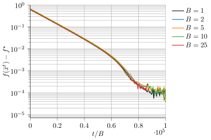
Figure 1: Numerical example: Evolution of the cost error normalized on the number of blocks.

5 Numerical example

We consider as a numerical example a learning problem in which agents have to classify samples belonging to two clusters. Formally, each agent $i\in\{1,\ldots,N\}$ has $m_{i}$ training samples $q_{i}^{1},\dots,q_{i}^{m_{i}}\in\mathbb{R}^{d}$ each of which has an associated binary label $b_{i}^{r}\in\{-1,1\}$ for all $r\in\{1,\ldots,m_{i}\}$. The goal of the agents is to compute in a distributed way a linear classifier from the training samples, i.e., to find a hyperplane of the form $\{z\in\mathbb{R}^{d}\mid\langle\theta,z\rangle+\theta_{0}=0\}$, with $\theta\in\mathbb{R}^{d}$ and $\theta_{0}\in\mathbb{R}$, which better separates the training data. For notational convenience, let $x=[\theta^{\top},\theta_{0}]^{\top}\in\mathbb{R}^{d+1}$ and $\hat{q}_{i}^{r}=[(q_{i}^{r})^{\top},1]^{\top}$. Then, the presented problem can be addressed by solving the following convex optimization problem, in which a regularized Hinge loss is used as cost function,

$$\mathop{\textrm{minimize}}_{x\in\mathbb{R}^{d+1}} \sum_{i=1}^{N}\frac{1}{m_{i}}\sum_{r=1}^{m_{i}}\max\left(0,1-b_{i}^{r}\langle x,\hat{q}_{i}^{r}\rangle\right)+\frac{\lambda}{2}\|x\|^{2},$$

where $\lambda>0$ is the regularization weight. This problem can be written in the form of (1) by defining $\xi_{i}^{r}=(\hat{q}_{i}^{r},b_{i}^{r})$ and

$$\mathbb{E}[h_{i}(x;\xi_{i})] =\frac{1}{m_{i}}\sum_{r=1}^{m_{i}}\left(\max\left(1-b_{i}^{r}\langle x,\hat{q}_{i}^{r}\rangle\right)+\frac{\lambda}{2N}\|x\|^{2}\right)$$

for all $i\in\{1,\ldots,N\}$. In fact, as long as each data $\xi_{i}^{r}$ is uniformly drawn from the dataset, Assumption  1(C) is satisfied. We implemented the algorithm in DISROPT [19] and we tested it in this scenario with $N=48$ agents, $x\in\mathbb{R}^{50}$ and different number of blocks, namely $B\in\{1,2,5,10,25\}$. We generated a synthetic dataset composed of $480$ points and assigned $10$ of them to each agent, i.e., $m_{1}=\dots=m_{N}=10$. Agents communicate according to a connected graph generated according to an Erdős-Rènyi random model with connectivity parameter $p=0.5$. The corresponding weight matrix is built by using the Metropolis-Hastings rule. Finally, we set $\lambda=1$, $p_{i,\ell}=1/B$ for all $i$ and all $\ell$, $p_{i,on}=0.95$ for all $i$ and local (constant) stepsizes $\alpha_{i}$ randomly chosen according to a normal distribution with mean $0.005$ and standard deviation $10^{-4}$. The evolution of the cost error adjusted with respect to the number of blocks is reported in Figure 1 for the considered block numbers. The linear convergence rate can be easily appreciated from the figure and confirms the theoretical analysis.

6 Conclusions

In this paper, we studied the behavior of the Distributed Block Proximal Method when applied to problems involving (non-smooth) strongly convex functions and when agents in the network employ constant stepsizes. A linear convergence rate (with a constant error) has been obtained in terms of the expected distance from the optimal cost. A numerical example involving a learning problem confirmed the theoretical analysis.

References

- [1] F. Farina and G. Notarstefano, “Randomized block proximal methods for distributed stochastic big-data optimization,” arXiv preprint arXiv:1905.04214, 2019.
- [2] ——, “A randomized block subgradient approach to distributed big data optimization,” in 2019 IEEE 58th Conference on Decision and Control (CDC), 2019, pp. 6362–6367.
- [3] B. Recht, “A tour of reinforcement learning: The view from continuous control,” Annual Review of Control, Robotics, and Autonomous Systems, vol. 2, no. 1, pp. 253–279, 2019.
- [4] L. Xiao, “Dual averaging methods for regularized stochastic learning and online optimization,” Journal of Machine Learning Research, vol. 11, no. Oct, pp. 2543–2596, 2010.
- [5] A. J. Kleywegt, A. Shapiro, and T. Homem-de Mello, “The sample average approximation method for stochastic discrete optimization,” SIAM Journal on Optimization, vol. 12, no. 2, pp. 479–502, 2002.
- [6] S. S. Ram, A. Nedić, and V. V. Veeravalli, “Distributed stochastic subgradient projection algorithms for convex optimization,” Journal of optimization theory and applications, vol. 147, no. 3, pp. 516–545, 2010.
- [7] A. Agarwal and J. C. Duchi, “Distributed delayed stochastic optimization,” in Advances in Neural Information Processing Systems, 2011, pp. 873–881.
- [8] K. Srivastava and A. Nedic, “Distributed asynchronous constrained stochastic optimization,” IEEE Journal of Selected Topics in Signal Processing, vol. 5, no. 4, pp. 772–790, 2011.
- [9] A. Nedić and A. Olshevsky, “Stochastic gradient-push for strongly convex functions on time-varying directed graphs,” IEEE Transactions on Automatic Control, vol. 61, no. 12, pp. 3936–3947, 2016.
- [10] J. Li, G. Li, Z. Wu, and C. Wu, “Stochastic mirror descent method for distributed multi-agent optimization,” Optimization Letters, vol. 12, no. 6, pp. 1179–1197, 2018.
- [11] B. Ying and A. H. Sayed, “Performance limits of stochastic sub-gradient learning, part ii: Multi-agent case,” Signal Processing, vol. 144, pp. 253–264, 2018.
- [12] I. Necoara, “Random coordinate descent algorithms for multi-agent convex optimization over networks,” IEEE Transactions on Automatic Control, vol. 58, no. 8, pp. 2001–2012, 2013.
- [13] R. Arablouei, S. Werner, Y.-F. Huang, and K. Doğançay, “Distributed least mean-square estimation with partial diffusion,” IEEE Transactions on Signal Processing, vol. 62, no. 2, pp. 472–484, 2013.
- [14] C. Wang, Y. Zhang, B. Ying, and A. H. Sayed, “Coordinate-descent diffusion learning by networked agents,” IEEE Transactions on Signal Processing, vol. 66, no. 2, pp. 352–367, 2017.
- [15] I. Notarnicola, Y. Sun, G. Scutari, and G. Notarstefano, “Distributed big-data optimization via block-wise gradient tracking,” arXiv preprint arXiv:1808.07252, 2018.
- [16] F. Farina, A. Garulli, A. Giannitrapani, and G. Notarstefano, “A distributed asynchronous method of multipliers for constrained nonconvex optimization,” Automatica, vol. 103, pp. 243 – 253, 2019.
- [17] C. D. Dang and G. Lan, “Stochastic block mirror descent methods for nonsmooth and stochastic optimization,” SIAM Journal on Optimization, vol. 25, no. 2, pp. 856–881, 2015.
- [18] H. H. Bauschke and J. M. Borwein, “Joint and separate convexity of the bregman distance,” in Inherently Parallel Algorithms in Feasibility and Optimization and their Applications, ser. Studies in Computational Mathematics. Elsevier, 2001, vol. 8, pp. 23 – 36.
- [19] F. Farina, A. Camisa, A. Testa, I. Notarnicola, and G. Notarstefano, “DISROPT: a Python Framework for Distributed Optimization,” arXiv e-prints, p. arXiv:1911.02410, 2019.