Learning in the Sky: An Efficient 3D Placement of UAVs

Abstract

Deployment of unmanned aerial vehicles (UAVs) as aerial base stations can deliver a fast and flexible solution for serving varying traffic demand. In order to adequately benefit of UAVs deployment, their efficient placement is of utmost importance, and requires to intelligently adapt to the environment changes. In this paper, we propose a learning-based mechanism for the three-dimensional deployment of UAVs assisting terrestrial cellular networks in the downlink. The problem is modeled as a noncooperative game among UAVs in satisfaction form. To solve the game, we utilize a low complexity algorithm, in which unsatisfied UAVs update their locations based on a learning algorithm. Simulation results reveal that the proposed UAV placement algorithm yields significant performance gains up to about $52\%$ and $74\%$ in terms of throughput and the number of dropped users, respectively, compared to an optimized baseline algorithm.

I Introduction

Due to the novel types of services and ongoing advances in unmanned aerial vehicle (UAV) technologies, there is a growing consensus on integrating UAVs into cellular networks. It is expected that UAVs will play a prominent role for traffic offloading, capacity enhancement and disaster recovery [1]. From an economic perspective, deploying small cell base stations (BSs) and/or advanced fifth generation (5G) components, such as massive multiple-input and multiple-output (MIMO), may not be cost-effective for temporary events. In this regard, deployment of UAVs can be considered as an alternative or complement solution. UAVs are able to establish line-of-sight (LoS) communication links with high probability for ground users resulting in increased coverage, enhanced reliability and agility [2].

Mobility of UAVs and their flexibility in adjusting their locations significantly impact the LoS probability and the network performance. Most research efforts have addressed this issue from a non-learning perspective [3, 2, 4]. However, there has been a growing attention recently devoted to the use of learning algorithms for the deployment problem of UAVs [5, 6, 7, 8]. In [5] and [6] learning based approaches to find the two-dimensional (2D) trajectory of UAVs flying with fixed altitudes were proposed. In [7], a learning based approach for three-dimensional (3D) placement of a single UAV is developed to maximize network throughput. However, these works do not address the 3D deployment of multiple UAVs integrated into already existing terrestrial networks. In [8], the problem of 3D placement was dealt as a two separate optimization problems in horizontal 2D plane and altitude of UAVs, where a prior knowledge of the users locations is required. However, providing this information for UAVs in real time can be challenging. Moreover, the proposed algorithm is not able to adapt to the environment changes. Finally, to our best knowledge, the channel models in the previous learning based reports do not capture the dependency of path loss exponents to the height of UAVs which might have a significant influence on the performance of UAVs [9, 2].

In this paper, we address the optimal 3D locations of multiple UAVs aiming to assist the existing terrestrial cellular networks. We formulate an optimization problem using a novel framework. This framework is based on a noncooperative game in satisfaction form which is implemented at the level of UAVs. Furthermore, as opposed to the related works, we take into account the network load effect, representing the BSs capabilities in serving users. Then, we leverage a learning based approach to develop a low complexity and robust algorithm allowing UAVs to autonomously adjust and optimize their locations adapted to dynamic environments. Finally, in order to examine our proposed algorithm, we employ a third generation partnership project (3GPP)-based height dependent channel model. Our findings from the simulation results show that the proposed learning based approach significantly improves the performance of the network, and reduces the required number of UAVs for an arbitrary target gain.

The rest of this paper is organized as follows. In Section II, we describe the system model. Section III presents the proposed algorithm for the 3D deployment of UAVs in the network. In Section IV, we evaluate the performance of the proposed approach. Finally, Section V concludes the paper.

II System Model

In this section, we describe the system model, including network topology, channel model, and user association method.

Network Topology: we consider the downlink of a cellular network consisting of a set of terrestrial BSs $\mathcal{M}$, and a set of UAVs $\mathcal{U}$ as aerial BSs to support the users in a particular area $\mathcal{R}\in\mathbb{R}^{2}$. The set of total users and the set of users associated to BS $b\in\mathcal{B}$ are denoted by $\mathcal{K}$ and $\mathcal{K}_{b}$, respectively, where $\mathcal{B}=\mathcal{M}\cup\mathcal{U}$ indicates the total BSs in the system. We assume that all the BSs transmit over the same channel, i.e. co-channel deployment. Let $\boldsymbol{a}_{b}(t)=(x_{b}(t),y_{b}(t),h_{b}(t))$ be the location of BS $b$ at time $t$, where $(x_{b}(t),y_{b}(t))$ and $h_{b}(t)$ are the location of BS $b$ in the horizontal dimension and its altitude at time $t$, respectively.

Radio Propagation and Signal Quality: we assume that the link between each user $k\in\mathcal{K}$ and each BS $b\in\mathcal{B}$ comprises LoS and non-LoS propagation conditions. Let $\mathrm{pr}_{bk}^{\mathrm{LoS}}(t)$ denote the probability of having a LoS link between user $k$ and BS $b$ at time $t$ which is determined as follows [9]:

$$\footnotesize\mathrm{pr}_{b,k}^{\mathrm{LoS}}(t)=\prod_{n=0}^{\lfloor\frac{r_{b,k}(t).\sqrt{\alpha.\beta}}{1000}-1\rfloor}\Bigg{[}1-\exp\Bigg{(}-\frac{{\Big{[}h_{b}-\frac{(n+\frac{1}{2})(h_{b}-h_{k})}{n+1}\Big{]}}^{2}}{2\gamma^{2}}\Bigg{)}\Bigg{]},$$ (1)

where $\alpha$, $\beta$ and $\gamma$ represent statistical environment-dependent parameters. Here, $h_{b}$ and $h_{k}$ are the altitude of BS $b$ and the altitude of user $k$, respectively. The horizontal location of user $k$, and its horizontal distance to BS $b$ at time $t$ are denoted by $(x_{k},y_{k})$ and $r_{b,k}(t)=\sqrt{(x_{b}(t)-x_{k})^{2}+(y_{b}(t)-y_{k})^{2}}$, respectively. Consequently, the non-LoS probability can be determined as $\mathrm{pr}_{b,k}^{\mathrm{NLoS}}(t)=1-\mathrm{pr}_{b,k}^{\mathrm{LoS}}(t)$.

Let $d_{b,k}(t)=\sqrt{r_{b,k}^{2}(t)+(h_{b}(t)-h_{k})^{2}}$ denote the 3D distance between BS $b$ and user $k$ at time $t$. The path loss between BS $b$ and user $k$ can be expressed as [9]:

$$L_{b,k}^{z}(t)=A_{b}^{z}+10\delta_{b,k}^{z}.\log_{10}(d_{b,k}(t)),$$ (2)

where superscript $z\in\{\mathrm{LoS},\mathrm{NLoS}\}$ denotes LoS and non-LoS components on the link. Here, $A_{b}^{z}$ and $\delta_{b,k}^{z}$ are the reference path loss and the path loss exponent, respectively. Therefore, the signal to interference plus noise ratio (SINR) experienced by user $k$ can be formulated as:

$$\gamma_{b,k}(t)=\frac{p_{b}(t)g_{b,k}^{z}(t)}{\sum_{b^{\prime}\in\mathcal{B}\backslash b}p_{b^{\prime}}(t)g_{b^{\prime},k}^{z^{\prime}}(t)+\sigma^{2}},$$ (3)

where $p_{b}(t)$ and $g_{b,k}^{z}(t)=10^{-\frac{L_{b,k}^{z}(t)}{10}}$ are the transmit power of BS $b$ and the channel gain between BS $b$ and user $k$, respectively. Parameter $\sigma^{2}$ represents the additive white Gaussian noise (AWGN) power.

The achievable data rate provided by BS $b$ to user $k$ using Shannon’s capacity formula is given by:

$$R_{b,k}(t)={\omega}\log_{2}(1+\gamma_{b,k}(t)),$$ (4)

where ${\omega}$ is the total bandwidth.

User Association Policy: we utilize a user association policy capturing both received signal power and load (which represents the BSs capabilities for serving new users). Let $\upsilon_{k}$ denote the traffic influx rate of user $k$. The fraction of time BS $b$ requires to serve the traffic $\upsilon_{k}$ to the location of user $k$ is defined as $\frac{\upsilon_{k}}{R_{b,k}(t)}$. Therefore, the load of BS $b$ at time $t$ is given by $\rho_{b}(t)=\sum_{k\in\mathcal{K}_{b}}\frac{\upsilon_{k}}{R_{b,k}(t)}$ [10].

To associate the users to the BSs we assume that each BS $b$ broadcasts its estimated load, ${\hat{\rho}}_{b}(t)$, at time $t$ which is obtained as follows[10]:

$${\hat{\rho}}_{b}(t)=\eta_{b}(t)\rho_{b}(t-1)+\Big{(}1-\eta_{b}(t)\Big{)}\hat{\rho}_{b}(t-1),$$ (5)

where $\eta_{b}(t)$ is the learning rate of the load estimation for BS $b$. Then, each user $k$ selects its serving BS based on the received signal power and the load of the BSs as follows [10]:

$$\begin{split}b_{k}(t)={\mathop{\arg\!\max}_{b\in\mathcal{B}}}\Big{\{}p_{b}(t)g_{b,k}^{z}(t){\left(1-\hat{\rho}_{b}(t)\right)}\Big{\}}.\end{split}$$ (6)

III Learning Based Placement Algorithm

In this section, we aim at optimizing the 3D locations of the UAVs for maximizing the throughput, without global network information. The problem of finding optimum 3D locations of the UAVs is complex mainly due to the mobility of the UAVs and temporal traffic statistics. Therefore, we leverage the tools of machine learning to solve the problem. In this regard, for each UAV $u\in\mathcal{U}$, a utility function is defined as follows:

$$\begin{split}f_{u}(t)=\phi_{u}.\frac{\sum_{k\in\mathcal{K}_{u}}R_{u,k}(t)}{\mu_{u}(t)}-\varphi_{u}.\Gamma_{u}(t),\end{split}$$ (7)

where $\phi_{u}$ and $\varphi_{u}$ are the weight parameters that indicate, respectively, the impact of throughput and the activation function $\Gamma_{u}(t)$ on the utility, and $\mu_{u}(t)$ is a normalization parameter. Here, $\Gamma_{u}(t)$ is an activation function for the safety of UAVs in order to avoid collision, which is defined as follows[5]:

$$\Gamma_{u}(t)=\begin{cases}1,&d_{u,u^{\prime}}<d_{\mathrm{min}},\ \ \forall u^{\prime}\neq u\\ 0,&\mbox{otherwise},\end{cases}$$ (8)

where $d_{u,u^{\prime}}$ and $d_{\mathrm{min}}$ represent the 3D distance between UAV $u$ and UAV $u^{\prime}$, and a certain minimum distance, respectively. According to (8), if the distance between UAV $u$ and UAV $u^{\prime}$ is less than a minimum distance $d_{\mathrm{min}}$, the function $\Gamma_{u}(t)$ returns value one which is considered as a cost in the utility function defined in (7). Let $\boldsymbol{A}(t)=(\boldsymbol{a}_{1}(t),\dots,\boldsymbol{a}_{|\mathcal{U}|}(t))$ denote the locations of the UAVs at time $t$. Therefore, the optimization problem is formulated as follows:

$$\max_{\boldsymbol{A}(t)}\leavevmode\nobreak\ \leavevmode\nobreak\ \sum_{t\in T}\sum_{u\in\mathcal{U}}f_{u}(t)$$ (9a)

s.t. $$(x_{u}(t),y_{u}(t))\in\mathcal{R},\quad\forall u\in\mathcal{U},$$ (9b)

$$h_{u}\in[h_{\mathrm{min}},h_{\mathrm{max}}],\quad\forall u\in\mathcal{U},$$ (9c)

$$0\leq\rho_{b}\leq 1,\quad\forall b\in\mathcal{B},$$ (9d)

where $T$ is the total working time of the UAVs. The parameters $h_{\mathrm{min}}$ and $h_{\mathrm{max}}$ denote the minimum and maximum altitude of the UAVs, respectively. For the optimization problem (9), the constraints in (9b)-(9c) define the feasible 3D space for the locations of the UAVs. The constraint in (9d) corresponds to the definition of load, in which it avoids outages and ensures service for the users in the network.

The problem of 3D deployment of the UAVs can be formulated as a noncooperative game in satisfaction form. In a satisfaction-form game, each UAV is interested in the satisfaction of its constraints. A game in satisfaction form can be described by the $\mathcal{G}=\left\langle\mathcal{U},\{\mathcal{S}_{u}\}_{u\in\mathcal{U}},\{c_{u}\}_{u\in\mathcal{U}}\right\rangle,$ where the set of the UAVs, $\mathcal{U}$, is considered as the set of players in the game. The set $\mathcal{S}_{u}$ denotes the set of strategies for UAV $u\in\mathcal{U}$. We define the set $\mathcal{S}_{u}$ as the movement in different directions: $\mathcal{S}_{u}=\{\mathrm{up,down,left,right,forward,backward,no\ change}\}$. Let $\boldsymbol{s}_{-u}$ be the strategies of all UAVs except UAV $u$. Here, the correspondence $c_{u}(\boldsymbol{s}_{-u})\subseteq\mathcal{S}_{u}$ denotes the set of strategies that can satisfy the constraints of UAV $u$ given the strategies played by all other UAVs. Therefore, the correspondence $c_{u}(\boldsymbol{s}_{-u})$ can be defined as follows [10]:

$$c_{u}(\boldsymbol{s}_{-u})=\{s_{u}\in\mathcal{S}_{u}:f_{u}(t)\geq\gamma_{u}\},$$ (10)

where $\gamma_{u}$ is the satisfaction threshold for UAV $u$. According to the observed utility, each UAV $u\in\mathcal{U}$ updates a satisfaction indicator $\vartheta_{u}(t)$ at time $t$ as follows:

$$\vartheta_{u}(t)=\begin{cases}1,&\mbox{if }s_{u}(t)\in c_{u}(\boldsymbol{s}_{-u})\\ 0,&\mbox{otherwise},\end{cases}$$ (11)

where $s_{u}(t)$ is the strategy of UAV $u$ at time $t$. For a game in satisfaction form, an important outcome is called satisfaction equilibrium where all players are satisfied, and $c_{u}(\boldsymbol{s}_{-u})$ is not empty for each player $u$. The notion of satisfaction equilibrium can be formulated as a fixed point as follows [10]:

Definition 1 (Satisfaction Equilibrium): A strategy profile $\boldsymbol{s}^{*}=(s_{u}^{*},\boldsymbol{s}_{-u}^{*})$ is a satisfaction equilibrium if $\forall u\in\mathcal{U}$, $s_{u}^{*}\in c_{u}(\boldsymbol{s}^{*}_{-u})$.

Algorithm 1 : Proposed algorithm for the 3D deployment of UAVs

1: Input: $t=0$, $\pi_{u,i}(t)$, $\vartheta_{u}(t-1)$, $\gamma_{u}$, $\forall u\in\mathcal{U}$ and $\forall s_{u,i}\in\mathcal{S}_{u}$.

2: Output: $\pi_{u,i}(t+1)$, $\vartheta_{u}(t)$, $\forall u\in\mathcal{U}$ and $\forall s_{u,i}\in\mathcal{S}_{u}$.

3: while $t<T$ do

4:    $t\leftarrow t+1$

5:    for each $u\in\mathcal{U}$ do

6:       if $\vartheta_{u}(t-1)=1$ then

7:          $s_{u}(t)=s_{u}(t-1)$,

8:       else

9:          Select a strategy $s_{u}(t)$ based on $\boldsymbol{\pi}_{u}(t)$,

10:       end if

11:       Update the location $\boldsymbol{a}_{u}(t)$ based on $s_{u}(t)$,

12:       Calculate utility $f_{u}(t)$ according to (7),

13:       Calculate $\vartheta_{u}(t)$ according to (11),

14:       Update $\boldsymbol{\pi}_{u}(t)$ according to (12),

15:    end for

16: end while

However, for a given satisfaction threshold, some UAVs may be faced with the situations where they can not be satisfied. Therefore, a satisfaction equilibrium may not always exist. In this context, we can reduce the satisfaction threshold $\gamma_{u}$ for unsatisfied UAVs after a certain time interval. Therefore, we use an adaptive threshold approach described in [10]. To solve the game in a distributed manner, we use a learning algorithm, and assume that each UAV $u$ can observe its obtained utility. If the UAV is satisfied with its current utility (i.e. $\vartheta_{u}(t)=1$), the UAV has no incentive to change its location. Otherwise, it may change its location according to the probability distribution $\boldsymbol{\pi}_{u}(t)=(\pi_{u,1}(t),\dots,\pi_{u,7}(t))$, where $\pi_{u,i}(t)$ is the probability assigned to strategy $s_{u,i}\in\mathcal{S}_{u}$ with $i\in\{1,\dots,7\}$. Therefore, each UAV $u$ updates the probability assigned to each strategy $s_{u,i}\in\mathcal{S}_{u}$ as follows [10]:

$$\pi_{u,i}(t+1)=\begin{cases}\pi_{u,i}(t),&\mbox{if }\vartheta_{u}(t)=1\\ L_{u}(\pi_{u,i}(t))&\mbox{otherwise}.\end{cases}$$ (12)

Here,

$${L_{u}\Big{(}\pi_{u,i}(t)\Big{)}=\pi_{u,i}(t)+\mu_{u}(t)q_{u}(t)\Big{(}\mathbbm{1}_{\{s_{u}(t)=s_{u,i}\}}-\pi_{u,i}(t)\Big{)},}$$ (13)

where $\mu_{u}(t)$ is the learning rate of UAV $u$. The parameter $q_{u}(t)$ is computed as $q_{u}(t)=\frac{f_{\mathrm{max}}+f_{u}(t)-\gamma_{u}}{2f_{\mathrm{max}}}$, where $f_{\mathrm{max}}$ is the maximum utility that UAV $u$ can achieve. The function $\mathbbm{1}_{\phi}$ denotes the indicator function which equals 1 if event $\phi$ is true and 0, otherwise.

The pseudocode for the proposed approach is presented in Algorithm 1. The algorithm converges to an equilibrium of the game $\mathcal{G}$ in finite time which is proved in  [10, Theorem 2].

Note that the proposed approach offers several distinct advantages. First, since only unsatisfied UAVs need to update their locations, it reduces the complexity, especially for deploying a multitude of UAVs. Second, due to the fact that our proposed algorithm can be executed in a distributed manner, the signaling overhead and exchanged information are expected to be negligible. Furthermore, it can gain the intrinsic advantage of distributed approaches such as improving network’s robustness against failures and attacks.

IV Simulation Results

To evaluate the performance of our proposed approach, we consider a hexagonal layout with radius $250$ m. The set of users are uniformly distributed in the area, and one terrestrial BS located in the center of the area. The simulation parameters are summarized in Table I. Furthermore, we demonstrate the performance gain of our proposed learning based scheme over the following benchmark references: 1) Strategic horizontal method proposed in [11] with fixed altitude $100$ m given ${79}$ predefined potential horizontal locations, referred to hereinafter as “strategic” approach. This approach is a heuristic approach, in which the horizontal location of a new UAV is determined from the predefined horizontal locations to achieve the furthest distances from the BSs in the system. 2) Random horizontal placement with fixed altitude $100$ m, referred to hereinafter as “random-fixed altitude” placement algorithm. 3) Random horizontal and altitude placement given ${79}$ and ${28}$ predefined potential horizontal and altitude locations, respectively, referred to hereinafter as “random” approach.

Table I: System-Level Simulation Parameters [9, 10]

System Parameters
Parameter		Value
Carrier frequency $(f_{c})$/ Channel bandwidth		$2$ GHz/ $10$ MHz
Noise power spectral density		$-174$ dBm/Hz
$\upsilon_{k}$		$1800$ Kbps
Learning rate exponent for $\eta_{b}(t)$		$0.9$
$d_{\mathrm{min}}$		$10$ m
$h_{\mathrm{min}},h_{\mathrm{max}}$		$22.5$ m, $300$ m
Altitude of users		$1.5$ m
Altitude of terrestrial BS		$25$ m
BS Parameters
Parameter	Terrestrial BS	UAV
Transmit power	$46$ dBm	$24$ dBm
Reference path loss (${f_{c}}$ in GHz)	LoS: $28+20\log_{10}(f_{c})$ NLoS: $13.54+20\log_{10}(f_{c})$	LoS: $30.9+20\log_{10}(f_{c})$ NLoS: $32.4+20\log_{10}(f_{c})$
Path loss exponent	LoS: $2.2$ NLoS: $3.9$	LoS: $2.225-0.05\log_{10}(h_{u})$ NLoS: $4.32-0.76\log_{10}(h_{u})$

Fig. 1 shows the average throughput per BS versus the number of users for a network with $8$ UAVs. The figure shows that the learning based UAV placement approach significantly improves the average throughput compared to the benchmark algorithms. For instance, for a network with $210$ users, the proposed approach improves the average throughput $51.82\%$, $84.35\%$, and $92.96\%$ compared to the strategic, random-fixed altitude, and random approaches, respectively. The main reason is that the UAVs adjust their locations in order to maximize the utility function defined in (7) which comprises their throughput.

Fig. 2 illustrates the average rate per user. We can observe that as the number of users increases, average rate per user decreases due to increasing load and the availability of limited resource in the network. Since the learning based approach optimize the locations of UAVs in terms of maximizing throughput, it improves the average rate of users compared to the benchmark algorithms

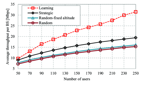
Figure 1: Average throughput per BS versus the number of users, given $8$ UAVs.

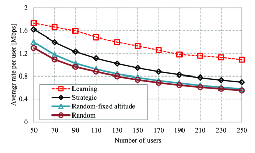
Figure 2: Average rate per user versus the number of users, given $8$ UAVs.

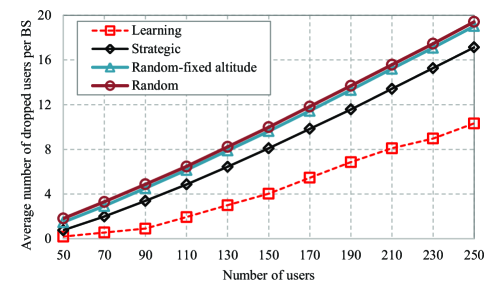
Figure 3: Average number of dropped users per BS versus the number of users, given $8$ UAVs.

In Fig. 3, we show the average number of dropped users per BS. The figure shows that the average number of dropped users increases with an increase in the number of users. This is mainly due to the fact that, a limited resource is available in the network. Therefore, with increasing the number of users, some of them may experience reductions in their rates due to the overloaded BSs. Since the proposed approach improves the average rate compared to the other approaches, it yields better performance in terms of average number of dropped users. The performance gain of the learning based approach compared to the strategic, random-fixed altitude, and random approaches is up to $74.14\%$, $86.76\%$, and $89.23\%$, respectively. Accordingly, the learning approach is more resistant to the higher traffic demand.

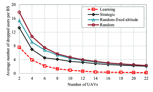
Figure 4: Average number of dropped users per BS versus the number of UAVs, given $100$ users.

Fig. 4 depicts the average number of dropped users as the number of UAVs varies. From the figure, as the number of UAVs increases the average number of dropped users per BS decreases. The main reason is that the users associated to the highly loaded BSs can be offloaded to the lightly loaded BSs. Moreover, Fig. 4 reveals that by using the learning based approach, the number of UAVs required to reduce the number of outage users below a certain threshold is significantly lower. For instance, using learning based method only $6$ UAVs are required for less than $2$ users in outage, which is notably lower than $22$ UAVs needed in the other methods.

V Conclusion

In this paper, we have proposed a low-complexity robust algorithm for the 3D placement of UAVs integrated into terrestrial cellular networks. The proposed approach leverages the tools from game theory and machine learning to learn optimal locations of UAVs in a distributed manner. Our results have shown that the proposed approach significantly outperforms the benchmark algorithms in terms of both throughput and dropped users. We have also shown that the number of UAVs for serving ground users using the learning based approach is significantly lower than the benchmark algorithms resulting in a more cost-effective networking with UAVs.

References

- [1] M. Mozaffari, W. Saad, M. Bennis, Y. Nam, and M. Debbah, “A tutorial on UAVs for wireless networks: Applications, challenges, and open problems,” IEEE Commun. Surveys Tuts., vol. 21, no. 3, pp. 2334–2360, 2019.
- [2] M. M. Azari, F. Rosas, K. Chen, and S. Pollin, “Ultra reliable UAV communication using altitude and cooperation diversity,” IEEE Trans. Commun., vol. 66, no. 1, pp. 330–344, 2018.
- [3] Z. Wang, L. Duan, and R. Zhang, “Adaptive deployment for UAV-aided communication networks,” IEEE Trans. Wireless Commun., vol. 18, no. 9, pp. 4531–4543, Sep. 2019.
- [4] M. Alzenad, A. El-Keyi, F. Lagum, and H. Yanikomeroglu, “3-D placement of an unmanned aerial vehicle base station (UAV-BS) for energy-efficient maximal coverage,” IEEE Wireless Commun. Lett, vol. 6, no. 4, pp. 434–437, 2017.
- [5] B. Khamidehi and E. S. Sousa, “Reinforcement learning-based trajectory design for the aerial base stations,” in 2019 IEEE 30th Annual International Symposium on PIMRC, 2019, pp. 1–6.
- [6] H. Dai, H. Zhang, M. Hua, C. Li, Y. Huang, and B. Wang, “How to deploy multiple UAVs for providing communication service in an unknown region?” IEEE Wireless Commun. Lett., vol. 8, no. 4, pp. 1276–1279, Aug 2019.
- [7] R. Ghanavi, E. Kalantari, M. Sabbaghian, H. Yanikomeroglu, and A. Yongacoglu, “Efficient 3D aerial base station placement considering users mobility by reinforcement learning,” in 2018 IEEE WCNC, April 2018, pp. 1–6.
- [8] H. El Hammouti, M. Benjillali, B. Shihada, and M. Alouini, “Learn-as-you-fly: A distributed algorithm for joint 3D placement and user association in multi-UAVs networks,” IEEE Trans. Wireless Commun., vol. 18, no. 12, pp. 5831–5844, Dec 2019.
- [9] M. M. Azari, G. Geraci, A. Garcia-Rodriguez, and S. Pollin, “UAV-to-UAV communications in cellular networks,” arXiv preprint arXiv:1912.07534, 2019.
- [10] A. Hajijamali Arani, M. J. Omidi, A. Mehbodniya, and F. Adachi, “Minimizing base stations’ ON/OFF switchings in self-organizing heterogeneous networks: A distributed satisfactory framework,” IEEE Access, vol. 5, pp. 26 267–26 278, 2017.
- [11] F. Lagum, I. Bor-Yaliniz, and H. Yanikomeroglu, “Strategic densification with UAV-BSs in cellular networks,” IEEE Wireless Commun. Lett, vol. 7, no. 3, pp. 384–387, 2018.